A Biorthogonal Hermite Cubic Spline Galerkin Method for Solving Fractional Riccati Equation

Abstract

This paper is devoted to the wavelet Galerkin method to solve the Fractional Riccati equation. To this end, biorthogonal Hermite cubic Spline scaling bases and their properties are introduced, and the fractional integral is represented based on these bases as an operational matrix. Firstly, we obtain the Volterra integral equation with a weakly singular kernel corresponding to the desired equation. Then, using the operational matrix of fractional integration and the Galerkin method, the corresponding integral equation is reduced to a system of algebraic equations. Solving this system via Newton’s iterative method gives the unknown solution. The convergence analysis is investigated and shows that the convergence rate is $O\left(2^{-s}\right)$. To demonstrate the efficiency and accuracy of the method, some numerical simulations are provided.

1. Introduction

One of the most important classes of nonlinear ordinary differential equations (ODEs) that plays a remarkable role in engineering, mathematics, and science is the Riccati equation. Count Riccati has studied the particular version of the Riccati equation for the first time in 1724. Since there is a close relationship between the homogeneous differential equation of the second-order and the Riccati equation, we can imagine many applications for this equation. This equation is closely related to the one-dimensional static Schrödinger equation and the solitary wave solution of nonlinear PDEs [1,2]. Furthermore, this equation also plays a vital role in modeling classical and modern dynamical systems [3,4].

In this paper, we focus on the wavelet Galerkin method, which used biorthogonal Hermite cubic Spline scaling bases (BHCSSb) as a set of bases to solve the fractional Riccati equation (FRE)

$${}^C{\mathcal{D}}_0^{\beta }u\left(x\right)=f\left(x\right)+g\left(x\right)u\left(x\right)+h\left(x\right)u^2\left(x\right),x\in [0,1],\beta \in {\mathbb{R}}^{+}$$

(1)

with initial condition

$$u^{\left(\eta \right)}\left(0\right)={\lambda }_{\eta },\eta =0,1,\dots ,n-1,$$

(2)

in which ${}^C{\mathcal{D}}_0^{\beta }u\left(x\right)$ is the Caputo fractional derivative and $\left[\beta \right]+1:=n\in \mathbb{N}$, for $\beta \notin \mathbb{N}$ and $n=\beta$ for $\beta \in \mathbb{N}$. Here, the functions f, g, and h are assumed to be continuous on $[0,1]$.

Because of the importance of this type of differential equation, several analytical and numerical methods have been used to solve it. In [5], the authors used new fractional bases based on the classical Legendre wavelet. In this work, the desired equation is solved using the operational matrix for Caputo fractional derivative and applying the Tau method. Rabiei et al. [6] introduced Boubaker wavelets of the fractional-order and used the collocation method to reduce the Riccati equation to a set of algebraic equations. The Jacobi collocation method is used to solve FRE in [7]. In [8], after representing the power function $t^{\alpha }$ based on the Bernstein series, the matrix form of the truncated Bernstein series of the fractional-order is obtained. Then, the operational matrix of the Caputo fractional derivative is obtained, and using the collocation method FRE is solved. Sequential quadratic programming and artificial neural networks are utilized to solve the problem [9]. We can also point to other methods to solve FRE, such as the variation of parameters method [10], the multipoint Padé approximation method [11], the Legendre collocation method [12], and the reproducing kernel method [13].

In several methods that are in the literature, to obtain accurate results, it is necessary to change a parameter that helps authors to convert the power of bases into fractions. This change is without prior knowledge and is randomly selected and can be different for each example. In our proposed method, the bases are not of the fractional-order. The employed method is based on BHCSSb, and it can be used efficiently to solve a variety of equations [14,15] via its properties. There are two types of wavelet systems, scaler wavelets, and multiwavelets. The scalar wavelet system is obtained using a single generator, while in the multi-wavelets system, the multiresolution spaces are spanned based on the multi-generator. Among the most important and widely used multiwavelets, we can mention Alpert’s multiwavelets [16,17,18] and biorthogonal Hermite cubic spline [15]. BHCSSb is a multiwavelet and uses two bases as the generator in multiresolution spaces.

As mentioned in the previous paragraph, our proposed method can solve a variety of ordinary and partial differential equations [14,15]. For this purpose, the corresponding integral equation must be obtained. By using the operational matrix of integral for this type of wavelet, as well as by using their interpolation property, the computational load will also decrease. This is one of the advantages of the method compared to the methods presented in the references [5,6,13].

Wavelets are used as a powerful tool for solving various equations. There are several excellent papers to show the ability of wavelets to solve a variety of equations, including the Burgers equation [19,20], conservation laws [21], Abel integral equation [17], generalized Cauchy problem [22], Nonlinear Partial Differential Equations [23], Boundary Value Problems [24], etc.

This paper is organized as follows: In Section 2, some basic preliminary and basic definitions about fractional calculus are presented. Then, biorthogonal Hermite cubic Spline scaling bases and their properties are introduced, and the operational matrix of the fractional integral is represented based on these bases. In the sequel, the wavelet Galerkin method is used to solve FRE, and the convergence analysis is investigated in Section 3. Section 4 is devoted to some numerical experiments.

2. Preliminaries

This section contains some preliminary definitions and properties of the Riemann–Liouville fractional integral and derivative and the Caputo fractional derivative. More details may be found in [25].

Definition 1.

Given $\beta \in {\mathbb{R}}^{+}$, let $\Gamma \left(\beta \right)$ is the Gamma function. The Riemann–Liouville fractional integral operator ${\mathcal{I}}_a^{\beta }$ of order β is determined by

$${\mathcal{I}}_a^{\beta }\left(u\right)\left(x\right):=\frac{1}{\Gamma \left(\beta \right)}{\int }_a^x{(x-\zeta )}^{\beta -1}u\left(\zeta \right)d\zeta ,x\in [a,b],u\in L_1[a,b],$$

(3)

where $[a,b]$ is a finite interval on $\mathbb{R}$.

It can be easy to directly verify that the fractional integration from the power functions is a yield power function of the same form, via

$${\mathcal{I}}_a^{\beta }\left(x^{\alpha }\right)=\frac{\Gamma (\alpha +1)}{\Gamma (\alpha +\beta +1)}{x}^{\alpha +\beta }.$$

(4)

It follows from [25] that the fractional integral operator ${\mathcal{I}}_a^{\beta }$ is bounded. To this end, we have the following Lemma.

Lemma 1.

(cf Lemma 2.1 (a), [25]). The operator ${\mathcal{I}}_a^{\beta }$ is bounded in $L_p\left([a,b]\right)$, i.e.,

$$\parallel {\mathcal{I}}_a^{\beta }{\left(u\right)\parallel }_p\le \frac{{(b-a)}^{\beta }}{\Gamma (\beta +1)}{\parallel u\parallel }_p,1\le p\le \infty .$$

(5)

Definition 2.

The Riemann–Liouville operator of the fractional derivative is defined by

$${}^R{\mathcal{D}}_a^{\beta }\left(u\right)\left(x\right):={\mathcal{D}}^n{\mathcal{I}}_a^{n-\beta }\left(u\right)\left(x\right)=\frac{1}{\Gamma (n-\beta )}{\mathcal{D}}^n{\int }_a^x{(x-\zeta )}^{n-\beta -1}u\left(\zeta \right)d\zeta ,$$

where $\alpha \in {\mathbb{R}}^{+}$, $\left[\alpha \right]+1:=n\in \mathbb{N}$ and ${\mathcal{D}}^n:=\frac{d^n}{d{x}^n}$.

Definition 3.

The Caputo fractional derivative is determined by [25,26].

$$\begin{array}{cc}\hfill {}^c{\mathcal{D}}_a^{\beta }\left(f\right)\left(x\right):& ==\frac{1}{\Gamma (n-\beta )}{\int }_a^x\frac{f^{\left(n\right)}\left(\zeta \right)d\zeta }{{(x-\zeta )}^{\beta -n+1}}=:{\mathcal{I}}_a^{n-\beta }{\mathcal{D}}^n\left(f\right)\left(x\right),\hfill \end{array}$$

(6)

in which $\beta \in {\mathbb{R}}^{+}$ and $\left[\beta \right]+1:=n\in \mathbb{N}$.

Lemma 2.

(cf Corollary 2.3 (a), [25]). It can be proved that the Caputo fractional derivative operator ${}^c{\mathcal{D}}_a^{\beta }$ is bounded via

$$\parallel {}^c{\mathcal{D}}_a^{\beta }{\left(f\right)\parallel }_C\le \frac{1}{\Gamma (n-\beta )(n-\beta +1)}{\parallel f\parallel }_{C^n},$$

(7)

where $\beta \in {\mathbb{R}}^{+}$, $\beta \notin {\mathbb{N}}_0$ and $n=-[-\beta ]$.

2.1. Biorthogonal Hermite Cubic Spline Scaling Bases

The biorthogonal Hermite cubic Spline scaling bases (BHCSSb) ${\psi }^1$ and ${\psi }^2$ are defined via

$${\psi }^1\left(x\right)=\left\{\begin{array}{cc}1-3x^2-2x^3,\hfill & x\in [-1,0],\hfill \\ 1-3x^2+2x^3,\hfill & x\in [0,1],\hfill \\ 0,\hfill & o.w,\hfill \end{array}\right.$$

(8)

and

$${\psi }^2\left(x\right)=\left\{\begin{array}{cc}x+2x^2+x^3,\hfill & x\in [-1,0],\hfill \\ x-2x^2+x^3,\hfill & x\in [0,1],\hfill \\ 0,\hfill & o.w.\hfill \end{array}\right.$$

(9)

It follows from [15] that ${\psi }^1,{\psi }^2\in C^1\left(\mathbb{R}\right)$ and fulfill Hermite interpolation

$${\psi }^1\left(x\right)={\delta }_{0,x},{\left({\psi }^1\right)}^{\prime }\left(x\right)=0,{\psi }^2\left(x\right)=0,{\left({\psi }^2\right)}^{\prime }\left(x\right)={\delta }_{0,x},\forall x\in \mathbb{Z},$$

(10)

where ${\delta }_{i,j}$ denotes the Kronecker delta.

Assume that the subspace $V_s\subset L_2\left(\mathbb{R}\right)$ is spanned by

$$V_s:=\{\sqrt{2}{\psi }_{s,0}^1{|}_{[0,1]},\sqrt{2}{\psi }_{s,2^s}^1{|}_{[0,1]}\}\bigcup \{{\psi }_{s,b}^k|b\in \mathcal{B},k=1,2\},$$

(11)

where $s\in {\mathbb{Z}}^{+}\cup \left\{0\right\}$, $\mathcal{B}:=\{1,\dots ,2^s-1\}$ and ${\psi }_{s,b}^k:={\psi }^k(2^s.-b)$. Motivated by the multiresolution properties [27], we know that these spaces are nested $V_s\subset V_{s+1}$. Thus, considering $\psi =({\psi }^1,{\psi }^2)$ as a vector function of the scaling function, it is easy to show that this vector satisfies the matrix refinement equation via,

$$\psi \left(x\right)=\sum _{b\in \mathbb{Z}}{H}_b\psi (2x-b),$$

(12)

in which

$$H_{-1}=\left(\begin{array}{cc}1/2& 3/4\\ -1/8& -1/8\end{array}\right),H_0=\left(\begin{array}{cc}1& 0\\ 0& 1/2\end{array}\right),H_1=\left(\begin{array}{cc}1/2& -3/4\\ 1/8& -1/8\end{array}\right),$$

(13)

and $\forall b\notin \{-1,0,1\}$, $H_b=O$ (O is the zero matrix). The vector function $\mathsf{\Psi }$ satisfies the following symmetry properties

$$\psi \left(x\right)=G\psi (-x),$$

(14)

where

$$G=\left(\begin{array}{cc}1& 0\\ 0& -1\end{array}\right).$$

Due to this relation, one can say that ${\psi }^1$ is symmetric and ${\psi }^2$ is antisymmetric. Using (13) and (14), we can write

$$H_b=G{H}_{-b}G,b\in \mathbb{Z}.$$

(15)

Because the Hermite cubic spline multiwavelet system is biorthogonal, there exists a dual multi-generator $\tilde{\psi }=({\tilde{\psi }}^1,{\tilde{\psi }}^2)$ that satisfies the biorthogonality condition, i.e.,

$$⟨\psi ,\tilde{\psi }(.-b)⟩={\delta }_{0,b}{I}_2,b\in \mathbb{Z},$$

(16)

where $I_2$ is the identity matrix of size two and $⟨.,.⟩$ denotes the $L_2$-inner product. This dual multi-generator generates another multiresolution space ${\tilde{V}}_s\subset L^2\left(\mathbb{R}\right)$, which is biorthogonal to $V_s$. In order to construct the dual scaling functions ${\tilde{\psi }}^1,{\tilde{\psi }}^2$, we utilize the refinement relation for primal and dual scaling functions and insert them into the biorthogonal relation (16). This gives rise to the discrete duality relation [15]

$$\sum _{l\in \mathbb{Z}}{H}_l{\tilde{H}}_{l+2b}^T=2{\delta }_{0,b}{I}_2,b\in \mathbb{Z}.$$

(17)

In which the refinement mask $\tilde{H}$ is chosen to be

$$\begin{array}{cc}\hfill {\tilde{H}}_{-2}& =\left(\begin{array}{cc}-\frac{7}{64}& -\frac{5}{64}\\ \frac{87}{128}& \frac{31}{64}\end{array}\right),{\tilde{H}}_{-1}=\left(\begin{array}{cc}\frac{1}{2}& \frac{3}{16}\\ -\frac{99}{32}& -\frac{37}{32}\end{array}\right),{\tilde{H}}_0=\left(\begin{array}{cc}\frac{39}{32}& 0\\ 0& \frac{15}{8}\end{array}\right),\hfill \\ \hfill {\tilde{H}}_1& =\left(\begin{array}{cc}\frac{1}{2}& -\frac{3}{16}\\ \frac{99}{32}& -\frac{37}{32}\end{array}\right),{\tilde{H}}_2=\left(\begin{array}{cc}-\frac{7}{64}& \frac{5}{64}\\ -\frac{87}{128}& \frac{31}{64}\end{array}\right),\hfill \end{array}$$

and ${\tilde{H}}_b=0$ for $b\notin -2,\dots ,2$.

By reindexing the scaling functions via the set $\phi =\{{\phi }_1,{\phi }_2,\dots ,{\phi }_{2^{s+1}}\}$, whose elements are equal to

$${\phi }_{2b+(k-1)}:={\psi }_{s,b}^k,fork=1,2,b\in \mathcal{B},$$

and ${\phi }_1:=\sqrt{2}{\psi }_{s,0}^1{|}_{[0,1]}$, ${\phi }_{2^{s+1}}:=\sqrt{2}{\psi }_{s,2^s}^1{|}_{[0,1]}$. Now, we introduce the operator ${\mathcal{P}}_s$ that is based on multi-scaling functions, which allows us to approximate any function $u\in L_2\left(\mathbb{R}\right)$ as follows

$$u\left(x\right)\approx {\mathcal{P}}_s\left(u\right)\left(x\right)=\sum _{l=1}^{2^{s+1}}{u}_l{\phi }_l\left(x\right),$$

(18)

where the coefficients $u_l=⟨u,{\phi }_l⟩$ for $l=1,\dots ,2^{s+1}$ are computed by using the Hermit type interpolation property of BHCSSb,

$$\left\{\begin{array}{cc}{u}_{2l}=u\left(\frac{l}{2^s}\right)\hfill & \\ u_{2l+1}=2^{-s}{u}^{\prime }\left(\frac{l}{2^s}\right)\hfill & l=1,\dots ,2^s-1,\hfill \\ u_1:=\frac{1}{\sqrt{2}}u\left(0\right),\hfill & \\ u_{2^{s+1}}:=\frac{1}{\sqrt{2}}u\left(1\right).\hfill \end{array}\right.$$

(19)

Now, for additional simplification, assume that ${\mathsf{\Psi }}_s$ is a vector function of dimension $2^{s+1}$ whose ith element is ${\phi }_i\left(x\right)$. Similarly, the vector U is chosen to be a vector of the same dimension of ${\mathsf{\Psi }}_s$ for which the ith element is $u_i$. According to this introduction, (18) can be rewritten via

$$u\left(x\right)\approx U^T{\mathsf{\Psi }}_s\left(x\right).$$

(20)

It follows from Theorem 2 in [14] that the error of approximation (18) can be bounded via the following theorem.

Theorem 1.

Let $u:[0,1]\to \mathbb{R}$ be a function in $C^4[0,1]$. The error resulting from the approximation ${\mathcal{P}}_s\left(u\right)$ is bounded as follows

$$\begin{array}{c}\hfill e_s\left(x\right):=|u\left(x\right)-{\mathcal{P}}_s\left(u\right)\left(x\right)|=\mathcal{C}{\mathcal{M}}_u\frac{2^{-s}}{1-2^{-1}},\end{array}$$

where $\mathcal{C}$ is a constant and ${\mathcal{M}}_u=max\{{max}_{\xi \in [0,1]}|u^{\left(2\right)}\left(\xi \right)|,{max}_{\xi \in [0,1]}|u^{\left(4\right)}\left(\xi \right)\left|\right\}$. Thus, we have

$$e_s\left(x\right)=O\left(2^{-s}\right).$$

Proof. 

See [14]. □

2.2. Representation of Fractional Integral Operator in BHCSSb

The fractional integration of the vector function ${\mathsf{\Psi }}_s\left(x\right)$ can be expressed by

$${\mathcal{I}}_0^{\beta }\left({\mathsf{\Psi }}_s\right)\left(x\right)\approx I_{\beta }{\mathsf{\Psi }}_s\left(x\right),$$

(21)

where $I_{\beta }$ is the Riemann–Liouville fractional integral operational matrix of dimension $N\times N$ with $N=2^{J+1}$.

To find the elements of matrix $I_{\beta }$, we continue the following process. Given $\beta \in {\mathbb{R}}^{+}$, the Riemann–Liouville fractional integral operator ${\mathcal{I}}_0^{\beta }$, acting on ${\psi }^k(2^{s}x-b)$ for $k=1,2$, can be represented by

$$\begin{array}{cc}\hfill {\mathcal{I}}_0^{\beta }\left({\psi }^k\right)(2^{s}x-b)& ={\displaystyle \frac{1}{\Gamma \left(\beta \right)}}{\int }_0^x{(x-\zeta )}^{\beta -1}{\psi }^k(2^s\zeta -b)d\zeta ,k=1,2,b\in \mathcal{B}.\hfill \end{array}$$

To evaluate this integral, we check out the four cases due to the support of ${\psi }^k(2^{s}x-b)$ for $k=1,2$.

• If $x\le \frac{b-1}{2^s}$, $b\in \mathcal{B}$ then according to the support of function ${\psi }^k(2^{s}x-b)$, it is easy to show that ${\mathcal{I}}_0^{\beta }\left({\psi }^k\right)(2^{s}x-b)=0$ for $k=1,2$.
• If $x\in (\frac{b-1}{2^s},\frac{b}{2^s})$, then we have

  $$\begin{array}{c}\hfill a_k(x,b):={\mathcal{I}}_0^{\beta }\left({\psi }^k\right)(2^{s}x-b)=\frac{1}{\Gamma \left(\beta \right)}{\int }_{\frac{b-1}{2^s}}^x{(x-\zeta )}^{\beta -1}{\psi }^k(2^s\zeta -b)d\zeta ,\mathrm{for}k=1,2.\end{array}$$
• If $x\in (\frac{b}{2^s},\frac{b+1}{2^s})$, then by putting $b_k(x,b):={\mathcal{I}}_0^{\beta }\left({\psi }^k\right)(2^{s}x-b)$, one can write

  $$\begin{array}{c}\hfill b_k(x,b)=\frac{1}{\Gamma \left(\beta \right)}\left({\int }_{\frac{b-1}{2^s}}^{\frac{b}{2^s}}{(x-\zeta )}^{\beta -1}{\psi }^k(2^s\zeta -b)d\zeta +{\int }_{\frac{b}{2^s}}^x{(x-\zeta )}^{\beta -1}{\psi }^k(2^s\zeta -b)d\zeta \right).\end{array}$$
• If $x\ge \frac{b+1}{2^s}$ then for $k=1,2$, we get

  $$\begin{array}{cc}\hfill c_k(x,b):={\mathcal{I}}_0^{\beta }\left({\psi }^k\right)(2^{s}x-b)& =\frac{1}{\Gamma \left(\beta \right)}\left({\int }_{\frac{b-1}{2^s}}^{\frac{b}{2^s}}{(x-\zeta )}^{\beta -1}{\psi }^k(2^s\zeta -b)d\zeta \right.\hfill \\ \hfill & \left.+{\int }_{\frac{b}{2^s}}^{\frac{b+1}{2^s}}{(x-\zeta )}^{\beta -1}{\psi }^k(2^s\zeta -b)d\zeta \right).\hfill \end{array}$$

The above integrals can be evaluated explicitly in terms of $\beta$, s, b for all values of $b\in \mathcal{B}$ for given $s\in {\mathbb{R}}^{+}$. We use a library function “int” available in Maple to evaluate the above integrals analytically. Thus, using the above-obtained integrals, the Riemann–Liouville fractional integral ${\mathcal{I}}_0^{\beta }\left({\psi }^k\right)(2^{s}x-b)$ is obtained as follows:

$$Q_k(x,b):={\mathcal{I}}_0^{\beta }\left({\psi }^k\right)(2^{s}x-b)=\left\{\begin{array}{cc}0,\hfill & x\le \frac{b-1}{2^s},\hfill \\ a_k(x,b),\hfill & \frac{b-1}{2^s}\le x<\frac{b}{2^s},\hfill \\ b_k(x,b),\hfill & \frac{b}{2^s}\le x<\frac{b+1}{2^s},\hfill \\ c_k(x,b),\hfill & x\ge \frac{b+1}{2^s}.\hfill \end{array}\right.$$

(22)

It follows from (22) that the fractional integration of vector function ${\mathsf{\Psi }}_s\left(x\right)$ takes the form

$${\mathcal{P}}_s{\mathcal{I}}_0^{\beta }\left({\mathsf{\Psi }}_s\right)\left(x\right)={\mathcal{P}}_s\left(P\left(x\right)\right)\approx I_{\beta }\left({\mathsf{\Psi }}_s\right)\left(x\right),$$

(23)

where $\Gamma \left(x\right)$ is a vector function whose elements are obtained via

$${\left[P\left(x\right)\right]}_{2b+(k+1)}:=Q_k(x,b),k=1,2,b\in \mathcal{B},$$

(24)

and

$$\begin{array}{cc}\hfill {\left[P\left(x\right)\right]}_1& :Q_1(x,0),\hfill \\ \hfill {\left[P\left(x\right)\right]}_{2^{s+1}}& :=Q_1(x,2^s).\hfill \end{array}$$

Now, we can find the entries of matrix $I_{\beta }$ through expanding each of the components of the vector function $\Gamma \left(x\right)$ by Biorthogonal Hermite cubic spline multi-scaling functions [14] as

$$\begin{array}{c}\hfill I_{\beta }=\left[\begin{array}{ccccccc}0\hfill & A\hfill & B_1\hfill & \cdots \hfill & \cdots \hfill & B_{2^{\mathsf{s}}-2}& E\\ & {\rm Y}\hfill & H_1\hfill & H_2\hfill & \cdots \hfill & H_{2^{\mathsf{s}}-2}& {\mathsf{\Delta }}_1\\ & & {\rm Y}\hfill & H_1\hfill & \cdots \hfill & H_{2^{\mathsf{s}}-3}& {\mathsf{\Delta }}_2\\ & & & \ddots \hfill & \ddots \hfill & ⋮& ⋮\\ & & & & {\rm Y}\hfill & H_1& ⋮\\ & & & & & {\rm Y}& {\mathsf{\Delta }}_{2^{\mathsf{s}}-1}\\ & & & & & & M\end{array}\right],\end{array}$$

(25)

where

$$\begin{array}{cc}\hfill M& ={\displaystyle \frac{6}{\Gamma (\beta +4)}}{2}^{-s\beta }(\beta +1),\hfill \\ \hfill E& =\frac{1}{\Gamma (\beta +4)}\left({(1-2^{-s})}^{\beta }(-12\left(2^{3s}\right)+12\beta \left(2^s\right)+(18-6\beta )2^{2s}-6\beta -6)+12\left(2^{3s}\right)\right.\hfill \\ \hfill & \left.-(18+6\beta )\times 2^{2s}+{\beta }^3+6{\beta }^2+11\beta +6\right),\hfill \end{array}$$

and

$$\begin{array}{cc}\hfill A& =\beta 2^{-s\beta +\frac{1}{2}}\left[\begin{array}{cc}{\displaystyle \frac{{\beta }^2+6\beta +5}{\Gamma (\beta +4)}}& {\displaystyle \frac{{\beta }^2+3\beta -4}{\Gamma (\beta +3)}}\end{array}\right],\hfill \\ \hfill B_{i-1}& =2^{-s\beta +\frac{1}{2}}\left[\begin{array}{cc}{\eta }_{1,1}^{i-1}& {\eta }_{1,2}^{i-1}\end{array}\right],i=2\dots ,2^s-1,\hfill \end{array}$$

with

$$\begin{array}{cc}\hfill {\eta }_{1,1}^{i-1}& =-\frac{2^{-s\beta +\frac{1}{2}}}{\Gamma (\beta +4)}\left(i^{\beta }(-11\beta -6-12i^3+(6\beta +18)i^2-{\beta }^3-6{\beta }^2)\right.\hfill \\ \hfill & \left.+{(i-1)}^{\beta }(6\beta +612i^3+(6\beta -18)i^2-12\beta i)\right),\hfill \\ \hfill {\eta }_{1,2}^{i-1}& =-\frac{2^{-s\beta +\frac{1}{2}}}{\Gamma (\beta +4)i}\left(i^{\beta }(12(\beta +3)i^3-6(6+{\beta }^2+5\beta )i^2+11{\beta }^2+6{\beta }^3+6\beta +{\beta }^4)\right.\hfill \\ \hfill & \left.+{(i-1)}^{\beta }(-12(\beta +3)i^3-6({\beta }^2+\beta -6)+6({\beta }^2+3\beta )i)\right),\hfill \end{array}$$

and the $2\times 2$ block matrices

$$\begin{array}{cc}\hfill {\rm Y}& =2^{-s\beta +1}\left[\begin{array}{cc}{\displaystyle \frac{3(\beta +1)}{\Gamma (\beta +4)}}& {\displaystyle \frac{3\beta }{\Gamma (\beta +3)}}\\ -{\displaystyle \frac{\beta }{\Gamma (\beta +4)}}& -{\displaystyle \frac{(\beta -1)}{\Gamma (\beta +3)}}\end{array}\right],\hfill \\ \hfill H_1& =2^{-s\beta +2}\left[\begin{array}{cc}{\displaystyle \frac{6(2^{\beta }(\beta -1)+1)}{\Gamma (\beta +4)}}& {\displaystyle \frac{3(2^{\beta }(\beta -2)+2)}{\Gamma (\beta +3)}}\\ -{\displaystyle \frac{2(\beta +3+2^{\beta }(\beta -3))}{\Gamma (\beta +4)}}& -{\displaystyle \frac{(2^{\beta }(\beta -4)+2\beta +4)}{\Gamma (\beta +3)}}\end{array}\right].\hfill \end{array}$$

The elements of the matrix $H_i=\left[\begin{array}{cc}{h}_{1,1}^i& h_{1,2}^i\\ h_{2,1}^i& h_{2,2}^i\end{array}\right]$, $i=1,\dots ,2^s-2,$ are denoted by

$$\begin{array}{cc}\hfill h_{1,1}^i& :=-6\frac{2^{(-s\beta )}}{\Gamma (\beta +4)}\left({(i-1)}^{\beta }(4-12i+2i^2-4i^3)+{(i-2)}^{\beta }(2i^3+(\beta -9)i^2-4(\beta -3)i+4\beta -4)\right.\hfill \\ \hfill & \left.+i^{\beta +2}(2i-(\beta +3))\right),\hfill \\ \hfill h_{1,2}^i& :=-6\frac{2^{(-s\beta )}}{\Gamma (\beta +3)}\left({(i-2)}^{\beta }(2i^2+(\beta -6)i-2\beta +4)+{(i-1)}^{\beta }(4i^2+8i-4)\right.\hfill \\ \hfill & \left.+i^{\beta }(2i^2-(\beta +2)i)\right),\hfill \\ \hfill h_{2,1}^i& :=-\frac{2^{(s\beta +1)}}{\Gamma (\beta +4)}\left(i^{\beta +2}(-3i+\beta +3)+{(i-1)}^{\beta }((12+4\beta )i^2-8i(\beta +3)+4\beta +12)\right.\hfill \\ \hfill & \left.+{(i-2)}^{\beta }(3i^3-(15-\beta )i^2-4(\beta -6)i+4\beta -12)\right),\hfill \\ \hfill h_{2,2}^i& :=-\frac{2^{(s\beta +1)}}{\Gamma (\beta +3)}\left({(i-2)}^{\beta }(3i^2+(\beta -10)i-2\beta +8)+{(i-1)}^{\beta }((8+4\beta )i-8-4\beta )\right.\hfill \\ \hfill & \left.+i^{\beta }(-3i^2+(\beta +2)\right).\hfill \end{array}$$

Finally, we introduce the matrices ${\mathsf{\Delta }}_i$, $i=1,\dots ,2^s-1$ as follows.

$$\begin{array}{c}\hfill {\mathsf{\Delta }}_i={\left[\begin{array}{cc}{\mu }_{1,1}^i& {\mu }_{1,2}^i\end{array}\right]}^T,i=1,\dots ,2^s-1,\end{array}$$

$$\begin{array}{cc}\hfill {\mu }_{1,1}^i& :=-{\displaystyle \frac{3\sqrt{2}}{\Gamma (\beta +4)}}\left({(\frac{3}{4}-\frac{1}{4}i)}^{\beta }(-2i^3+(\beta +21)i^2+9\beta +81-6(\beta +12)i)+{(1-\frac{1}{4}i)}^{\beta }(4i^3-48i^2\right.\hfill \\ \hfill & \left.+192i-256)+{(\frac{5}{4}-\frac{1}{4}i)}^{\beta }(-2i^3+(27-\beta )i^2-10(12-\beta )i-25\beta +175)\right),\hfill \\ \hfill {\mu }_{1,2}^i& :=-{\displaystyle \frac{\sqrt{2}}{\Gamma (\beta +4)}}\left({(\frac{3}{4}-\frac{1}{4}i)}^{\beta }(9\beta +108-(6\beta +99)i+(\beta +30)i^2-3i^3)+{(1-\frac{1}{4}i)}^{\beta }(4(\beta +3)i^2\right.\hfill \\ \hfill & \left.-32(\beta +3)i+192+64\beta )+{(\frac{5}{4}-\frac{1}{4}i)}^{\beta }(3i^3+(\beta -42)i^2+(-10\beta +195)i+25\beta -300)\right).\hfill \end{array}$$

Lemma 3.

Let $f_s\left(x\right):=C^T{\mathsf{\Psi }}_s\left(x\right)$ be the approximation of $f\in L^2[0,1]$ based on BHCSSb. If ${\mathcal{I}}_0^{\beta }\left(f_s\right)\left(x\right)$ is obtained by $C^T{I}_{\beta }{\mathsf{\Psi }}_s\left(x\right)$, then we have

$$\underset{s\to \infty }{lim}{\mathcal{I}}_0^{\beta }\left(f_s\right)\left(x\right)={\mathcal{I}}_0^{\beta }\left(f\right)\left(x\right).$$

(26)

Proof. 

It follows from Theorem 1 that

$$\underset{s\to \infty }{lim}{f}_s\left(x\right):=\underset{s\to \infty }{lim}{\mathcal{P}}_s\left(f\right)\left(x\right)=\underset{s\to \infty }{lim}\sum _{i=1}^{2^{s+1}}{c}_i{\phi }_i\left(x\right)=f\left(x\right).$$

(27)

Since ${\phi }_i\left(x\right)\in C[0,1]$ for $i=1,\dots ,2^{s+1}$, one can write

$$\underset{s\to \infty }{lim}{\int }_0^x{(x-t)}^{\beta -1}\sum _{i=1}^{2^{s+1}}{c}_i{\phi }_i\left(t\right)dt=\underset{s\to \infty }{lim}\sum _{i=1}^{2^{s+1}}{c}_i{\int }_0^x{(x-t)}^{\beta -1}{\phi }_i\left(t\right)dt.$$

(28)

Thus, we can write

$$\underset{s\to \infty }{lim}{\mathcal{I}}_0^{\beta }\left(f_s\right)\left(x\right)=\underset{s\to \infty }{lim}{C}^T{I}_{\beta }{\mathsf{\Psi }}_s\left(x\right).$$

(29)

By (29) and from the Definition 1 for $\beta \in {\mathbb{R}}^{+}$, we have

$$\Gamma \left(\beta \right){\mathcal{I}}_0^{\beta }\left(f\right)\left(x\right)={\int }_0^x{(x-t)}^{\beta -1}f\left(t\right)dt=\underset{s\to \infty }{lim}{\int }_0^x{(x-t)}^{\beta -1}{f}_s\left(t\right)dt=\Gamma \left(\beta \right)\underset{s\to \infty }{lim}{C}^T{I}_{\beta }{\mathsf{\Psi }}_s\left(x\right).$$

(30)

Consequently, using (29) and (30) we have

$$\underset{s\to \infty }{lim}{\mathcal{I}}_0^{\beta }\left(f_s\right)\left(x\right)={\mathcal{I}}_0^{\beta }\left(f\right)\left(x\right).$$

□

3. Wavelet Galerkin Method

In the present section, we utilize the wavelet Galerkin method based on BHCSSb to solve the Riccati Equation (1). To derive the approximate solution, we suppose that the unknown solution can be approximated by

$$u\left(x\right)\approx U^T{\mathsf{\Psi }}_s\left(x\right),$$

(31)

where U is a vector of dimension N that should be determined. Assume that $\beta \in {\mathbb{R}}^{+}$, $n=-[-\alpha ]$, and f, g, and h are continuous functions. Then, it is easy to show that the function $u\left(x\right)$ is a solution of the Riccati Equation (1), if, and only if, it satisfies the integral equation

$$u\left(x\right)=\sum _{\eta =0}^{n-1}\frac{u^{\left(\eta \right)}\left(0\right)}{\eta !}{x}^{\eta }+{\mathcal{I}}_0^{\beta }\left(f+gu+h{u}^2\right)\left(x\right).$$

(32)

Using (31), we can approximate all terms in the right side of (1) as follows

$$\begin{array}{cc}\hfill h\left(x\right)u^2\left(x\right)\approx & H^T{\mathsf{\Psi }}_s\left(x\right),\hfill \\ \hfill g\left(x\right)u\left(x\right)\approx & G^T{\mathsf{\Psi }}_s\left(x\right),\hfill \\ \hfill f\left(x\right)\approx & F^T{\mathsf{\Psi }}_s\left(x\right),\hfill \end{array}$$

(33)

Inserting Equation (33) into (32) and using the operational matrix of fractional integration $I_{\beta }$, we have the residual as follows

$$r\left(x\right)=\left(U^T-X^T-F^T{I}_{\beta }-G^T{I}_{\beta }-H^T{I}_{\beta }\right){\mathsf{\Psi }}_s\left(x\right),$$

(34)

in which $X\left(x\right):={\sum }_{\eta =0}^{n-1}\frac{u^{\left(\eta \right)}\left(0\right)}{\eta !}{x}^{\eta }\approx X^T{\mathsf{\Psi }}_s\left(x\right)$. We would like to reduce the residual to zero. There are several methods to do this. However, in this work, we use the wavelet Galerkin method. The biorthogonality of BHCSSb ($⟨{\mathsf{\Psi }}_s,\widetilde{{\mathsf{\Psi }}_s}⟩$) yields the linear or nonlinear system

$$\mathcal{F}\left(U\right)=0,$$

(35)

where $\mathcal{F}$ is a vector function of U. This function may be linear or nonlinear, and it depends on the function h. To find the unknown vector U, we utilize Newton’s method in the nonlinear type and the generalized minimal residual method (GMRES method) [28] in the linear type.

4. Convergence Analysis

Theorem 2.

Given $\beta \in {\mathbb{R}}^{+}$, let $\mathbb{N}\ni n=-[-\beta ]$. Let f, g and h be sufficiently smooth functions on $[0,1]$. The error of the wavelet Galerkin method based on BHCSSb for Equation (1) satisfies

$$\parallel u-u_s{\parallel }_{\infty }=O\left(2^{-s}\right).$$

(36)

Proof. 

If $f\left(x\right)$ is a continuous function, we can directly find the following error via Theorem 1

$$\begin{array}{cc}\hfill \parallel {\mathcal{I}}_0^{\beta }f-{\mathcal{I}}_0^{\beta }{\mathcal{P}}_s\left(f\right)\parallel & \le C_1{\mathcal{M}}_f\frac{2^{-s}}{\Gamma \left(\beta \right)(1-2^{-1})}\parallel {\int }_0^x{(x-\zeta )}^{\beta -1}d\zeta \parallel \hfill \\ \hfill & =C_1{\mathcal{M}}_f\frac{2^{-s}}{\beta \Gamma \left(\beta \right)(1-2^{-1})},\hfill \end{array}$$

where $C_1$ is a constant and ${\mathcal{M}}_f=max\{{max}_{\xi \in [0,1]}|f^{\left(2\right)}\left(\xi \right)|,{max}_{\xi \in [0,1]}|f^{\left(4\right)}\left(\xi \right)\left|\right\}$. Since the functions g and h are continuous, then there exist a constant $C_2$ such that $max\{g,h\}\le C_2$. It follows from Lemma 1 that

$$\parallel {\mathcal{I}}_0^{\beta }\left(gu\right)-{\mathcal{I}}_0^{\beta }{\mathcal{P}}_s\left(gu\right)\parallel \le \frac{C_2}{\Gamma (\beta +1)}\parallel u-u_s\parallel ,$$

(37)

and

$$\parallel {\mathcal{I}}_0^{\beta }\left(h{u}^2\right)-{\mathcal{I}}_0^{\beta }{\mathcal{P}}_s\left(h{u}^2\right)\parallel \le \frac{C_3}{\Gamma (\beta +1)}\parallel u-u_s\parallel ,$$

(38)

where $C_3=C_2\lambda$ with $\parallel u^2-u_s^2\parallel \le \lambda \parallel u-u_s\parallel$.

Subtracting (32) from

$$u_s=X_s+{\mathcal{I}}_0^{\beta }\left({\mathcal{P}}_s(f+gu+h{u}^2)\right)\left(x\right),$$

(39)

we have

$$u-u_s=X-X_s+{\mathcal{I}}_0^{\beta }\left(f+gu+h{u}^2\right)\left(x\right)-{\mathcal{I}}_0^{\beta }\left({\mathcal{P}}_s(f+gu+h{u}^2)\right)\left(x\right).$$

(40)

Taking the norm from both sides of (40) and using the triangle inequality, it follows from Theorem 1 that

$$\begin{array}{cc}\hfill \parallel u-u_s\parallel & \le C_0{\mathcal{M}}_X\frac{2^{-s}}{(1-2^{-1})}+C_1{\mathcal{M}}_f\frac{2^{-s}}{\beta \Gamma \left(\beta \right)(1-2^{-1})}+\frac{C_2}{\Gamma (\beta +1)}\parallel u-u_s\parallel \hfill \\ \hfill & +\frac{C_3}{\Gamma (\beta +1)}\parallel u-u_s\parallel ,\hfill \end{array}$$

where $\parallel X-{\mathcal{P}}_s\left(X\right)\parallel \le C_0{\mathcal{M}}_X\frac{2^{-s}}{(1-2^{-1})}$ with ${\mathcal{M}}_X=max\{{max}_{\xi \in [0,1]}|X^{\left(2\right)}\left(\xi \right)|,{max}_{\xi \in [0,1]}|X^{\left(4\right)}\left(\xi \right)\left|\right\}$. Therefore, if $C_4:=1-\frac{C_2+C_3}{\Gamma (\beta +1)}>0$ then

$$\parallel u-u_s\parallel \le C{2}^{-s},$$

in which $C=1/C_{4}max\{C_0{\mathcal{M}}_X,\frac{1}{\Gamma (\beta +1)}{C}_1{\mathcal{M}}_f\}$. □

5. Numerical Experiments

Example 1.

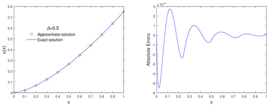
Consider the fractional Riccati equation

$${}^C{\mathcal{D}}_0^{\beta }u\left(x\right)+u^2\left(x\right)={\left(\frac{x^{\beta +1}}{\Gamma (\beta +2)}\right)}^2,x\in [0,1],$$

subject to the initial condition $u\left(0\right)=0$. The exact solution is reported in [6] and is $u\left(x\right)=\frac{x^{\beta +1}}{\Gamma (\beta +2)}$.

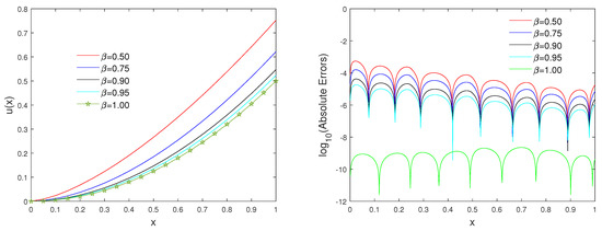
Table 1 shows a comparison between our proposed method and the Bernoulli wavelets method [29]. We observe that the wavelet Galerkin method based on BHCSSb gives better results than the Bernoulli wavelets method. To illustrate the effect of refinement level s on $L_2$-errors, Table 2 is reported. It is worth emphasizing that these results verify our convergence analysis, and by increasing this parameter, the $L_2$-errors decrease. To show the accuracy of the method, Figure 1 is plotted. In this figure, we can see a compare between the exact and approximate solutions. Figure 2 demonstrates the approximate solutions for different values of β on the left side and corresponding absolute errors on the right.

Table 1. The comparison between the proposed method and the Bernoulli wavelets method [29], taking $\beta =0.8$ for Example 1.

	Proposed Method		Bernoulli Wavelets Method [29]
	$\mathit{N}=\mathbf{9}$	$\mathit{N}=\mathbf{17}$	$\mathit{N}=\mathbf{28}$
$0.1$	$4.52\times {10}^{-5}$	$7.76\times {10}^{-6}$	$2.00\times {10}^{-6}$
$0.2$	$2.68\times {10}^{-5}$	$2.75\times {10}^{-6}$	$2.94\times {10}^{-6}$
$0.3$	$1.02\times {10}^{-5}$	$2.54\times {10}^{-6}$	$2.86\times {10}^{-6}$
$0.4$	$8.81\times {10}^{-6}$	$1.30\times {10}^{-7}$	$1.51\times {10}^{-6}$
$0.5$	$1.33\times {10}^{-5}$	$3.10\times {10}^{-8}$	$3.97\times {10}^{-4}$
$0.6$	$8.86\times {10}^{-6}$	$1.32\times {10}^{-6}$	$3.60\times {10}^{-4}$
$0.7$	$5.76\times {10}^{-6}$	$8.68\times {10}^{-7}$	$3.24\times {10}^{-4}$
$0.8$	$2.85\times {10}^{-6}$	$4.04\times {10}^{-7}$	$2.85\times {10}^{-4}$
$0.9$	$8.84\times {10}^{-7}$	$3.39\times {10}^{-6}$	$2.40\times {10}^{-4}$
$1.0$	$5.29\times {10}^{-6}$	$5.19\times {10}^{-6}$	$1.76\times {10}^{-4}$

Table 2. The effect of parameter s on $L_2$-errors for Example 1.

	$\mathit{s}=1$	$\mathit{s}=2$	$\mathit{s}=3$	$\mathit{s}=4$	$\mathit{s}=5$
$L_2$-error	$5.31\times {10}^{-4}$	$1.36\times {10}^{-4}$	$3.41\times {10}^{-5}$	$1.22\times {10}^{-5}$	$8.23\times {10}^{-6}$

Figure 1. Comparing the approximate and exact solutions, taking $s=2$ and $\beta =0.5$, for Example 1.

Figure 2. Comparing the approximate and exact solutions, taking $s=2$ and different values of $\beta$, for Example 1.

Example 2.

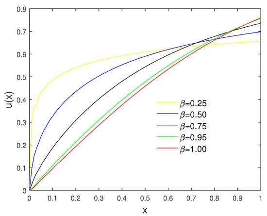
The second example is dedicated to the fractional Riccati equation

$${}^C{\mathcal{D}}_0^{\beta }u\left(x\right)+u^2\left(x\right)=1,x\in [0,1],$$

subject to the initial condition $u\left(0\right)=0$. There is no exact solution to the problem here. However, in the case of $\beta =1$, the exact solution would form $u\left(x\right)=\frac{e^{2x}-1}{e^{2x}+1}$ [5,6].

Figure 3 displays the approximate solution for different values of β. As we expect, when $\beta =1$, the corresponding solutions tend to the solution at it. Table 3 shows a comparison of the proposed method and the fractional-order Legendre wavelet method [5].

Figure 3. The approximate solution, taking $s=4$ and different values of $\beta$, for Example 2.

Table 3. Comparison of the absolute value of residual between the proposed method and fractional-order Legendre wavelet method [5] for Example 2.

		$\mathit{\beta }=0.25$	$\mathit{\beta }=0.50$	$\mathit{\beta }=0.75$
fractional-order Legendre wavelet method	$r=6$	$9.6\times {10}^{-4}$	$9.7\times {10}^{-4}$	$5.4\times {10}^{-4}$
	$r=10$	$8.5\times {10}^{-5}$	$6.0\times {10}^{-6}$	$4.0\times {10}^{-7}$
proposed method	$r=2$	$2.1\times {10}^{-25}$	$1.1\times {10}^{-26}$	$1.0\times {10}^{-23}$

Example 3.

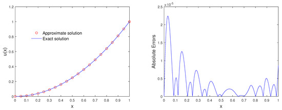
Consider the fractional Riccati equation

$${}^C{\mathcal{D}}_0^{0.5}u\left(x\right)=\frac{8}{3\sqrt{\pi }}{x}^{\frac{3}{2}}+x^2+x^4-u\left(x\right)-u^2\left(x\right),x\in [0,1],$$

subject to the initial condition $u\left(0\right)=0$. The exact solution is reported in [6] and is $u\left(x\right)=x^2$.

Figure 4 illustrates a comparison between the exact and approximate solution. The absolute errors are reported in Table 4.

Figure 4. Comparing the approximate and exact solutions, taking $s=3$, for Example 3.

Table 4. The absolute error for $s=3$ for Example 3.

	$\mathit{x}=0.2$	$\mathit{x}=0.4$	$\mathit{x}=0.6$	$\mathit{x}=0.8$	$\mathit{x}=1.0$
Absolute Errors	$1.79\times {10}^{-6}$	$3.93\times {10}^{-6}$	$1.75\times {10}^{-6}$	$1.26\times {10}^{-7}$	$8.63\times {10}^{-6}$

6. Conclusions

In this paper, we applied the wavelet Galerkin method to solve the fractional Riccati equation. To this end, we utilized the Biorthogonal cubic Hermite spline multiwavelets and the operational matrix for fractional integration to reduce the desired equation to a set of nonlinear algebraic systems. The convergence analysis is investigated and shows that the convergence rate is $O\left(2^{-s}\right)$. Some numerical simulations and results demonstrate the ability and efficiency of the method.

References

- Conte, R.; Musette, M. Link between solitary waves and projective Riccati equations. J. Phys. A Math. Gen. 1992, 25, 5609–5623. [Google Scholar] [CrossRef]
- Kravchenko, V. Applied Pseudo Analytic Function Theory, ch. 6 Complex Riccati Equation, 65–72 Frontiers in Mathematics; Brikhauser: Basel, Switzerland, 2009. [Google Scholar] [CrossRef]
- Mainardi, F.; Pagnini, G.; Gorenflo, R. Some aspects of fractional diffusion equations of single and distributed orders. Appl. Math. Comput. 2007, 187, 295–305. [Google Scholar] [CrossRef] [Green Version]
- Wu, J.L.; Chen, G.H. A new operational approach for solving fractional calculus and fractional differential equations numerically. In Proceedings of the Seventh IASTED International Conference on Software Engineering and Applications, Marina del Rey, CA, USA, 3–5 November 2003. [Google Scholar]
- Mohammadi, F.; Cattani, C. A generalized fractional-order Legendre wavelet Tau method for solving fractional differential equations. J. Comput. Appl. Math. 2018, 339, 306–316. [Google Scholar] [CrossRef]
- Rabiei, K.; Razzaghi, M. Fractional-order Boubaker wavelets method for solving fractional Riccati differential equations. Appl. Num. Math. 2021, 168, 221–234. [Google Scholar] [CrossRef]
- Singh, H.; Srivastava, H.M. Jacobi collocation method for the approximate solution of some fractional-order Riccati differential equations with variable coefficients. Phys. A Stat. Mech. Its Appl. 2019, 523, 1130–1149. [Google Scholar] [CrossRef]
- Yuzbasi, S. Numerical solutions of fractional Riccati type differential equations by means of the Bernstein polynomials. Appl. Math. Comput. 2013, 219, 6328–6343. [Google Scholar]
- Raja, M.A.Z.; Manzar, M.A.; Samar, R. An efficient computational intelligence approach for solving fractional order Riccati equations using ANN and SQP. Appl. Math. Model. 2015, 39, 3075–3093. [Google Scholar] [CrossRef]
- Haq, E.U.; Ali, M.; Khan, A.S. On the solution of fractional Riccati differential equations with variation of parameters method. Eng. Appl. Sci. Lett. 2020, 3, 1–9. [Google Scholar]
- Jeng, S.W.; Kilicman, A. Fractional Riccati equation and its applications to Rough Heston model using numerical methods. Symmetry 2020, 12, 959. [Google Scholar] [CrossRef]
- Kashkari, B.S.H.; Syam, M.I. Fractional-order Legendre operational matrix of fractional integration for solving the Riccati equation with fractional order. Appl. Math. Comput. 2016, 290, 281–291. [Google Scholar] [CrossRef]
- Li, X.; Wu, B.; Wang, R. Reproducing kernel method for fractional Riccati differential equations. Abstr. Appl. Anal. 2014, 970967. [Google Scholar] [CrossRef] [Green Version]
- Ashpazzadeh, E.; Lakestani, M. Biorthogonal cubic Hermite spline multiwavelets on the interval for solving the fractional optimal control problems. Comput. Methods Differ. Equ. 2016, 4, 99–115. [Google Scholar]
- Dahmen, W.; Han, B.; Jia, R.Q.; Kunoth, A. Biorthogonal multiwavelets on the interval: Cubic Hermite splines. Constr. Approx. 2000, 16, 221–259. [Google Scholar] [CrossRef] [Green Version]
- Alpert, B.; Beylkin, G.; Coifman, R.R.; Rokhlin, V. Wavelet-like bases for the fast solution of second-kind integral equations. SIAM J. Sci. Stat. Comput. 1993, 14, 159–184. [Google Scholar] [CrossRef]
- Saray, B.N. Abel’s integral operator: Sparse representation based on multiwavelets. BIT Numer. Math. 2021, 61, 587–606. [Google Scholar] [CrossRef]
- Saray, B.N. An effcient algorithm for solving Volterra integro-differential equations based on Alpert’s multi-wavelets Galerkin method. J. Comput. Appl. Math. 2019, 348, 453–465. [Google Scholar] [CrossRef]
- Alpert, B.; Beylkin, G.; Gines, D.; Vozovoi, L. Adaptive solution of partial differential equations in multiwavelet bases. J. Comput. Phys. 2002, 182, 149–190. [Google Scholar] [CrossRef] [Green Version]
- Saray, B.N.; Lakestani, M.; Dehghan, M. On the sparse multiscale representation of 2–D Burgers equations by an efficient algorithm based on multiwavelets. Numer. Meth. Part. Differ. Equ. 2021. [Google Scholar] [CrossRef]
- Hovhannisyan, N.; Müller, S.; Schäfer, R. Adaptive multiresolution discontinuous Galerkin schemes for conservation laws. Math. Comp. 2014, 83, 113–151. [Google Scholar] [CrossRef] [Green Version]
- Asadzadeh, M.; Saray, B.N. On a multiwavelet spectral element method for integral equation of a generalized Cauchy problem. BIT Numer. Math. 2022, 1–34. [Google Scholar] [CrossRef]
- Beylkin, G.; Keiser, J.M. On the Adaptive Numerical Solution of Nonlinear Partial Differential Equations in Wavelet Bases. J. Comput. Phys. 1997, 132, 233–259. [Google Scholar] [CrossRef] [Green Version]
- Dahmen, W.; Kunoth, A.; Schneider, R. Wavelet Least Squares Methods for Boundary Value Problems. SIAM J. Numer. Anal. 2002, 39, 1985–2013. [Google Scholar] [CrossRef]
- Kilbas, A.; Srivastava, H.M.; Trujillo, J.J. Theory and Applications of Fractional Differential Equations, 24; Elsevier, B.V.: Amsterdam, The Netherlands, 2006. [Google Scholar]
- Afarideh, A.; Dastmalchi Saei, F.; Lakestani, M.; Saray, B.N. Pseudospectral method for solving fractional Sturm-Liouville problem using Chebyshev cardinal functions. Phys. Scr. 2021, 96, 125267. [Google Scholar] [CrossRef]
- Mallat, S.G. A Wavelet Tour of Signal Processing; Academic Press: Cambridge, MA, USA, 1999. [Google Scholar]
- Saad, Y.; Schultz, M.H. GMRES: A generalized minimal residual method for solving nonsymmetric linear 165 systems. SIAM J. Sci. Stat. Comput. 1986, 7, 856–869. [Google Scholar] [CrossRef] [Green Version]
- Rahimkhani, P.; Ordokhani, Y.; Babolian, E. Fractional-order Bernoulli wavelets and their applications. Appl. Math. Model. 2016, 40, 8087–8107. [Google Scholar] [CrossRef]
Publisher’s Note: MDPI stays neutral with regard to jurisdictional claims in published maps and institutional affiliations. |
© 2022 by the authors. Licensee MDPI, Basel, Switzerland. This article is an open access article distributed under the terms and conditions of the Creative Commons Attribution (CC BY) license (https://creativecommons.org/licenses/by/4.0/).