A D-Optimal Sequential Calibration Design for Computer Models

Abstract

The problem with computer model calibration by tuning the parameters associated with computer models is significant in many engineering and scientific applications. Although several methods have been established to estimate the calibration parameters, research focusing on the design of calibration parameters remains limited. Therefore, this paper proposes a sequential computer experiment design based on the D-optimal criterion, which can efficiently tune the calibration parameters while improving the prediction ability of the calibrated computer model. Numerical comparisons of the simulated and real data demonstrate the efficiency of the proposed technique.

1. Introduction

Experiments are conducted to explore or optimize physical phenomena. In some applications, such as national defense, medicine, and manufacturing, the physical experiments may be difficult to be conducted due to economic, technical, or ethical limitations. To reduce the experimental cost, mathematical models, which are also called computer models, are developed to mimic, understand, and predict the physical phenomena in many applications [1,2,3]. The computer models are useful and efficient only if they can approximate the physical process well. Oftentimes, the computer models contain a set of calibration parameters, which are physical unobservable variables. The computer models’ fidelity to physical process relies on the unknown values of calibration parameters. Then, physical data and computer model outputs are combined to estimate the calibration parameters such that the computer model matches the physical process. This procedure is referred to as computer model calibration in the literature.

Numerous models have been proposed in the literature for the problem of computer model calibration, such as [2,4,5,6,7]. Among them, the Kennedy and O’Hagan model is the most commonly used. The Kennedy and O’Hagan model integrates the physical data and computer model outputs through a Bayesian framework. Any posterior quantity can serve as the point estimate of calibration parameter depending on the loss function specified. In practice, the most commonly used predictor of the physical process is a calibrated computer model, see [8,9]. Since the nonlinear effects from the discrepancy function can be hard to interpret and also may open up the possibility of overfitting with limited physical observations. Ref. [10] pointed out that an interpretable calibration parameter should allow the computer model to predict the real physical phenomena well even without the discrepancy function.

How to perform the experiments efficiently to tune the calibration parameters accurately under some metrics plays an important role. Although we are not the first to look into the problem of design for calibration, it has not received enough attention. Based on the Kennedy and O’Hagan model, some designs have been proposed in the literature. Ref. [11] employed the Kullback–Liebler (KL) divergence criterion as a function of the computer model inputs and obtained the estimate of calibration parameters by minimizing this criterion. Ref. [12] focused on the problem of functional calibration by generating sequential designs for the physical and computer experiments. Ref. [13] used results from the nonlinear optimal design theory to design such experiments. Ref. [14], based on the Kennedy and O’Hagan model, proposed an optimal sequential design for both computer and physical experiments by regarding integrated mean squared prediction error. Based on the Bayesian model calibration framework of [6], a D-optimal design for the physical experiment was proposed by [15]. Ref. [16] proposed a follow-up optimal experiment design for computer models calibration. In some practices, no physical experiments can be conducted after the initial design due to limitations. Thus, these designs, considering the physical experiments, are hard and impracticable. Ref. [17] presented an adaptive design for computer experiments to estimate the calibration parameters by using the expected improvement (EI) algorithm. It aims at reducing the calibration error induced by the uncertainty of the emulator of computer models but not at improving the estimation of calibration parameters. Inspired by this, we divert effort on the designs only considering computer experiments to estimate the calibration parameters. The D-optimal criterion is well known and widely used in the literature, which can help gather more information about the calibration parameters by minimizing the asymptotic variances of estimate. This paper proposes a sequential computer experiment calibration design using the D-optimal criterion and presents a fast algorithm to generate the designs.

The article is organized as follows. Section 2 reviews the Kennedy and O’Hagan calibration method. In Section 3, the proposed local D-optimal sequential design is presented. A fast algorithm for generating the corresponding designs is suggested. In Section 4, some simulation studies are made to demonstrate the performance of the proposed design. Conclusions and remarks are given in Section 5. Appendix A shows the derivation of the Fisher Information Matrix (FIM) for the calibration parameters.

2. Calibration of Computer Models

An important reference for computer calibration is the work of [6]. In this section, we will review some related background about the Kennedy and O’Hagan model. Let $y^p$ be the observation of physical process and $\mathit{x}=(x_1,\cdots ,x_r)\in \mathcal{X}\subset {\mathit{R}}^r$ be the control variables, which are also the set of inputs for physical process. According to [6], the physical observation $y^p$ can be modeled as

$$\begin{array}{c}\hfill y^p(\mathit{x})=y^c(\mathit{x},\mathit{\theta })+\delta (\mathit{x})+ϵ,\end{array}$$

(1)

where $y^c(·,·)$ is a computer model, $\mathit{\theta }\in \mathcal{T}\subset R^h$ is the set of calibration parameters, $\delta (·)$ is the discrepancy function which is independent of the computer model $y^c(·,·)$; $ϵ\sim N(0,{\lambda }^2)$ is the observation error and ${\lambda }^2$ is the corresponding variance. In the literature, the most popular methods to fit the computer model $y^c(·,·)$ and discrepancy function $\delta (·)$ are the Gaussian processes due to analytical tractability. Thus, the prior information about both $y^c(·,·)$ and $\delta (·)$ is considered as

$$\begin{array}{cc}\hfill & y^c(·,·)\sim GP(m(·,·),c_1\{(·,·),(·,·)\}),\hfill \\ \hfill & \delta (·)\sim GP(0,c_2(·,·)),\hfill \end{array}$$

(2)

where $m(·,·)$ is the mean function of computer model. Assume $\mathit{x}$ and ${\mathit{x}}^{\prime }$ denote the values of control inputs, and $\mathit{t}$ and ${\mathit{t}}^{\prime }$ denote the values of calibration inputs. According to the literature [18,19], $c_1\{(·,·),(·,·)\}$ and $c_2(·,·)$ are usually the corresponding separable covariance functions such as    

$$\begin{array}{cc}\hfill & c_1\{(\mathit{x},\mathit{t}),({\mathit{x}}^{\prime },{\mathit{t}}^{\prime })\}={\sigma }_1^{2}exp\left\{-{(\mathit{x}-{\mathit{x}}^{\prime })}^T{\mathsf{\Omega }}_x^{-1}(\mathit{x}-{\mathit{x}}^{\prime })\right\}exp\left\{-{(\mathit{t}-{\mathit{t}}^{\prime })}^T{\mathsf{\Omega }}_{\theta }^{-1}(\mathit{t}-{\mathit{t}}^{\prime })\right\},\hfill \\ \hfill & c_2(\mathit{x},{\mathit{x}}^{\prime })={\sigma }_2^{2}exp\left\{-{(\mathit{x}-{\mathit{x}}^{\prime })}^T{\mathsf{\Omega }}_{\delta }^{-1}(\mathit{x}-{\mathit{x}}^{\prime })\right\}.\hfill \end{array}$$

(3)

Here, ${\sigma }_1^2$ and ${\sigma }_2^2$ are the variance parameters,

$$\begin{array}{c}\hfill {\mathsf{\Omega }}_x=diag\{{\omega }_x^1,{\omega }_x^2,\cdots ,{\omega }_x^r\}\\ \hfill {\mathsf{\Omega }}_{\theta }=diag\{{\omega }_{\theta }^1,{\omega }_{\theta }^2,\cdots ,{\omega }_{\theta }^h\}\end{array}$$

and

$$\begin{array}{c}\hfill {\mathsf{\Omega }}_{\delta }=diag\{{\omega }_{\delta }^1,{\omega }_{\delta }^2,\cdots ,{\omega }_{\delta }^r\}.\end{array}$$

In terms of the mean function $m(·,·)$, the linear model structure is always considered, i.e.,

$$\begin{array}{c}\hfill m(\mathit{x},\mathit{t})=\mathit{h}{(\mathit{x},\mathit{t})}^{\mathit{T}}\mathit{\beta },\end{array}$$

(4)

where $\mathit{h}(\mathit{x},\mathit{t})={(h_1(\mathit{x},\mathit{t}),h_2(\mathit{x},\mathit{t}),\cdots ,h_p(\mathit{x},\mathit{t}))}^T$ is a vector of p known functions over $\mathcal{X}$ and $\mathit{\beta }={({\beta }_1,{\beta }_2,\cdots ,{\beta }_p)}^T$ is the corresponding unknown regression coefficients.

Let ${\mathcal{D}}^p=\{{\mathit{x}}_1^p,{\mathit{x}}_2^p,\cdots ,{\mathit{x}}_q^p\}$ be the design for physical experiment with q points, ${\mathit{y}}^p={\{y_1^p,y_2^p,\cdots ,y_q^p\}}^T$ be the corresponding physical outputs,

$${\mathcal{D}}^c=\{({\mathit{x}}_1^c,{\mathit{t}}_1^c),({\mathit{x}}_2^c,{\mathit{t}}_2^c),\cdots ,({\mathit{x}}_n^c,{\mathit{t}}_n^c)\}$$

be the design for computer experiment with n points, and ${\mathit{y}}^c={\{y_1^c,y_2^c,\cdots ,y_n^c\}}^T$ be the corresponding computer outputs. Thus, the full output $\mathit{d}={({\mathit{y}}^{cT},{\mathit{y}}^{pT})}^T$ is normally distributed given $(\mathit{\theta },\mathit{\beta },{\sigma }_1^2,{\sigma }_2^2,{\lambda }^2,{\mathsf{\Omega }}_x,{\mathsf{\Omega }}_{\mathit{\theta }},{\mathsf{\Omega }}_{\delta })$, and the corresponding likelihood function can be yielded. In order to express the mean and variance matrix of full output clearly, we define the following notations. Let ${\mathit{\psi }}_1=({\sigma }_1^2,{\mathsf{\Omega }}_x,{\mathsf{\Omega }}_{\mathit{\theta }}), {\mathit{\psi }}_2=({\sigma }_2^2,{\mathsf{\Omega }}_{\delta })$, $\mathit{\phi }=({\lambda }^2,{\mathit{\psi }}_1,{\mathit{\psi }}_2)$ and ${\mathcal{D}}_{\mathit{\theta }}^p=\{({\mathit{x}}_1^p,\mathit{\theta }),({\mathit{x}}_2^p,\mathit{\theta }),\cdots ,({\mathit{x}}_q^p,\mathit{\theta })\}$ be the augmented design points by calibration parameters $\mathit{\theta }$. Then the mean and variance matrix for full output vector $\mathit{d}$ given $(\mathit{\theta },\mathit{\beta },\mathit{\phi })$ can be derived as

$$\begin{array}{c}\hfill E(\mathit{d}|\mathit{\theta },\mathit{\beta },\mathit{\phi })=\mathit{H}(\mathit{\theta })\mathit{\beta },\end{array}$$

(5)

and

$$\begin{array}{c}\hfill var(\mathit{d}|\mathit{\theta },\mathit{\beta },\mathit{\phi })=\left(\begin{array}{cc}{V}_1({\mathcal{D}}^c)& C_1({\mathcal{D}}^c,{\mathcal{D}}_{\theta }^p)\\ C_1({\mathcal{D}}^c,{\mathcal{D}}_{\theta }^p)& \lambda {\mathit{I}}_q+V_1({\mathcal{D}}_{\theta }^p)+V_2({\mathcal{D}}^p)\end{array}\right),\end{array}$$

(6)

where $V_1({\mathcal{D}}^c)$ is the variance matrix of ${\mathit{y}}^c$ with $(i,j)$ element

$$c_1\{({\mathit{x}}_i^c,{\mathit{t}}_i^c),({\mathit{x}}_j^c,{\mathit{t}}_j^c)\},$$

$i,j\in \{1,2,\cdots ,n\}$; $C_1({\mathcal{D}}^c,{\mathcal{D}}_{\mathit{\theta }}^p)$ is the matrix with $(i,j)$ element

$$c_1\{({\mathit{x}}_i^c,{\mathit{t}}_i^c),({\mathit{x}}_j^p,\mathit{\theta })\},$$

$i\in \{1,\cdots ,n\},j\in \{1,\cdots ,q\}$; $V_1({\mathcal{D}}_{\theta }^p)$ and $V_2({\mathcal{D}}^p)$ are defined similar with $V_1({\mathcal{D}}^c)$; and ${\mathit{I}}_q$ is a $q\times q$ identity matrix. Then the posterior for the parameters given the data can be written as

$$\begin{array}{c}\hfill p(\mathit{\theta },\mathit{\beta },\mathit{\phi }|\mathit{d},{\mathcal{D}}^c,{\mathcal{D}}_{\mathit{\theta }}^p)\propto p(\mathit{d}|\mathit{\theta },\mathit{\beta },\mathit{\phi })\pi (\mathit{\theta },\mathit{\beta },\mathit{\phi }),\end{array}$$

(7)

where $\pi (\mathit{\theta },\mathit{\beta },\mathit{\phi })$ is the prior for unknown parameters. The MCMC techniques are usually used to determine the posterior distribution, but require complex computations. To simplify the computations, we adopt the modularization by the literature [20], namely, first estimate the emulator of the computer model and then the discrepancy.

The modular approach in [20] is considered here to estimate the parameters in the model, which can be described as follows. The maximum likelihood estimates (MLEs) $\widehat{\mathit{\beta }}$ of $\mathit{\beta }$ and ${\widehat{\mathit{\psi }}}_1$ of ${\mathit{\psi }}_1$ can be obtained based on the computer experimental data $({\mathcal{D}}^c,{\mathit{y}}^c)$. For the calibration parameter $\mathit{\theta }$, which is a tuning parameter, there is no “true value”. The goal of calibration is to find out some type of best-fitting value of $\mathit{\theta }$. It is easy to obtain the least-squares estimate of $\mathit{\theta }$, i.e., the value $\tilde{\mathit{\theta }}$ that minimizes the differences between the physical outputs and the computer model outputs by regarding fixing the $\mathit{\beta }$ and ${\mathit{\psi }}_1$ at their MLEs. The bias data $({\mathcal{D}}^p,{\mathit{y}}^p-{\widehat{\mathit{y}}}^c({\mathcal{D}}_{\tilde{\mathit{\theta }}}^p))$ can be employed to compute the MLEs ${\widehat{\mathit{\psi }}}_2$ of ${\mathit{\psi }}_2$ and $\widehat{\lambda }$ of $\lambda$, where ${\widehat{\mathit{y}}}^c({\mathcal{D}}_{\tilde{\mathit{\theta }}}^p))$ is the prediction from the surrogate model. Then, considering the MLEs $\widehat{\mathit{\beta }}$ and $\widehat{\mathit{\phi }}$ as fixed values, the posterior mean $\widehat{\mathit{\theta }}$ of the calibration parameters $\mathit{\theta }$ is deduced according to the prior information and observation data. As pointed out by [8], despite the maximum likelihood estimate plug-in being only approximately Bayesian, the resulting answers seem to be close to those from a full Bayesian analysis.

3. Sequential D-Optimal Design for Calibration Parameters

How to design the physical and computer experiments efficiently is critical to calibrating the computer models. Usually, the design for the physical and computer experiments is conducted separately in practice. A space-filling design is oftentimes used as the initial design for computer experiments, and some uniform designs or factorial designs are employed for physical experiments. Due to the limitation of physical experiments, after the initial designs, only computer experiments are considered to improve the estimation of calibration parameters sequentially. Here, we propose a sequential D-optimal design for computer experiments, which improves the estimation by maximizing the determinant of the FIM.

3.1. D-Optimal Criterion

Following the model presented in Section 2, full output vector $\mathit{d}$ is normally distributed given $(\mathit{\theta },\mathit{\beta },\mathit{\phi })$. Thus, the FIM can be derived as

$$\begin{array}{c}\hfill I(\mathit{\theta })=\int -(\frac{{\partial }^2}{\partial {\mathit{\theta }}^2}ln(p(\mathit{d}|\mathit{\theta },\mathit{\beta },\mathit{\phi })))p(\mathit{d}|\mathit{\theta },\mathit{\beta },\mathit{\phi })d\mathit{d},\end{array}$$

(8)

where $p(\mathit{d}|\mathit{\theta },\mathit{\beta },\mathit{\phi })$ is the conditional distribution density function, also known as the likelihood function. Similar to [15,21], the formula of FIM of the calibration parameter is presented in the following lemma. The process of the derivation is shown in Appendix A.

Lemma 1.

Let $\mathit{d}|\mathit{\theta },\mathit{\beta },\mathit{\phi }$ be distributed as $GP(H(\mathit{\theta })\mathit{\beta },var(\mathit{d}|\mathit{\theta },\mathit{\beta },\mathit{\phi }))$. Then, the $(i,j)$th element of the FIM is

$$\begin{array}{cc}\hfill & I_{ij}(\mathit{\theta })=\frac{\partial {(H(\mathit{\theta })\mathit{\beta })}^T}{\partial {\mathit{\theta }}_i}{(var(\mathit{d}|\mathit{\theta },\mathit{\beta },\mathit{\phi }))}^{-1}\frac{\partial (H(\mathit{\theta })\mathit{\beta })}{\partial {\mathit{\theta }}_j}+\hfill \\ \hfill & \frac{1}{2}tr\left({(var(\mathit{d}|\mathit{\theta },\mathit{\beta },\mathit{\phi }))}^{-1}\frac{\partial (var(\mathit{d}|\mathit{\theta },\mathit{\beta },\mathit{\phi }))}{\partial {\mathit{\theta }}_j}{(var(\mathit{d}|\mathit{\theta },\mathit{\beta },\mathit{\phi }))}^{-1}\frac{\partial (var(\mathit{d}|\mathit{\theta },\mathit{\beta },\mathit{\phi }))}{\partial {\mathit{\theta }}_i}\right].\hfill \end{array}$$

(9)

where $tr(·)$ is the trace of the matrix, and $i,j\in \{1,\cdots ,h\}$.

The corresponding D-optimal design is generated by maximizing

$$\begin{array}{c}\hfill {\mathcal{D}}_{\mathit{\theta }}=arg\underset{\mathcal{D}\in \mathcal{X}}{max}log\left|I(\mathit{\theta })\right|,\end{array}$$

(10)

which is similar to [22,23], where $\mathcal{X}$ denotes the experimental space, and $|·|$ is the determinant of a matrix. The inverse of FIM is the asymptotic variance matrix of the estimate of calibration parameters. Thus, maximizing (10) is equivalent to minimizing the volume of the confidence ellipsoid of the estimate, which can help improve the estimation. Obviously, it is not an easy task to create a D-optimal design by maximizing (10) directly. Here, we utilize the one-point-at-a-time strategy, i.e., add the computer design points by using the D-optimal criterion sequentially, which is referred to as sequential D-optimal design hereafter in this paper.

3.2. Algorithm for Generating Sequential D-Optimal Design

Let ${\mathcal{D}}^p$ and ${\mathcal{D}}^c$ be the initial designs for physical and computer experiments, respectively. In the process of the $i$th iteration, assume ${\mathcal{D}}^s=\{({\mathit{x}}_1^s,{\widehat{\mathit{\theta }}}_0),({\mathit{x}}_2^s,{\widehat{\mathit{\theta }}}_1),\cdots ,({\mathit{x}}_i^s,{\widehat{\mathit{\theta }}}_{i-1})\}$ be the computer experimental points generated sequentially, and ${\mathit{y}}^s=\{y_1^s,y_2^s,\dots ,y_i^s\}$ be the corresponding computer outputs. Then the estimate ${\widehat{\mathit{\theta }}}_i$ can be obtained based on the current full data $\{({\mathcal{D}}^c,{\mathit{y}}^c),({\mathcal{D}}^s,{\mathit{y}}^s),({\mathcal{D}}^p,{\mathit{y}}^p)\}$. For a fair comparison, the stopping rule is set as ‘$i\ge N$’, where N is the prefixed number of the sequential design points. Then, the next computer experiment point is selected by maximizing

$$\begin{array}{c}\hfill {\mathit{x}}_{i+1}^s=\underset{\mathit{x}\in \mathcal{X}}{argmax}log{\left|I(\mathit{\theta })\right|}_{\mathit{\theta }={\widehat{\mathit{\theta }}}_i,\mathit{\beta }=\widehat{\mathit{\beta }},\mathit{\phi }=\widehat{\mathit{\phi }}}.\end{array}$$

(11)

Evaluate the computer model at $({\mathit{x}}_{i+1}^s,{\widehat{\mathit{\theta }}}_i)$ and denote the output as $y_{i+1}^s$. The sequential design is augmented as ${\mathcal{D}}^s={\mathcal{D}}^s\cup \{({\mathit{x}}_{i+1}^s,{\widehat{\mathit{\theta }}}_i)\}$, and the corresponding computer outputs are augmented as ${\mathit{y}}^s={\mathit{y}}^s\cup \{y_{i+1}^s\}$. The value ${\widehat{\mathit{\theta }}}_N$ is used as the final estimate of calibration parameter $\mathit{\theta }$. Note that it is an r-dimensional optimization problem to find out the next computer experiment point by maximizing (11), which is a challenge. In order to overcome this problem, discrete optimization is commonly performed. For example, [16] used an algorithm (e.g., [24]) based on a fine grid of the r-dimensional input space. Ref. [17] used a greedy fashion scheme, in which the calibration parameter estimate was considered as the value that maximized the EI criterion over a grid. However, a greedy search based on fine grids may be time-consuming. We employ the following procedure to search for the next design point. Let $\mathcal{C}$ be a space-filling design with k points over computer experimental space $\mathcal{X}$ and $f_{{\widehat{\mathit{\theta }}}_i}(c_l)=log{\left|I(\mathit{\theta })\right|}_{\mathit{\theta }={\widehat{\mathit{\theta }}}_i,\mathit{x}={\mathit{c}}_{\mathit{l}}}$ be the corresponding logarithm value of the determinant of FIM at $c_l$ and ${\widehat{\mathit{\theta }}}_i$. It is generally reasonable that $k=500$ for $r<5$ and $k={10}^r$ or ${20}^r$ for $r\ge 5$, which is similar to [25]. In the numerical simulation studies in Section 4 and the real data analysis in Section 5, since $r\le 3$, then $k=500$ is a reasonable choice. Based on $\mathcal{C}$ and the corresponding evaluations, we can calculate $f_{{\widehat{\mathit{\theta }}}_i}(·)$. Then, the next computer experiment point is selected by maximizing

$$\begin{array}{c}\hfill {\mathit{x}}_{i+1}^s=\underset{\mathit{x}\in \mathcal{C}}{argmax}{f}_{{\widehat{\mathit{\theta }}}_i}(\mathit{x}).\end{array}$$

(12)

The details about the algorithm to create the sequential D-optimal design are presented as Algorithm 1.

Algorithm 1: Algorithm for Generating Sequential D-optimal Design

Input: Given physical observation data {${\mathcal{D}}^p=({\mathit{x}}_1^p,\dots ,{\mathit{x}}_q^p),{\mathit{y}}^p$}, initial computer     experiment data {${\mathcal{D}}^c=(({\mathit{x}}_1^c,{\mathit{t}}_1^c),\dots ,({\mathit{x}}_n^c,{\mathit{t}}_n^c)),{\mathit{y}}^c$}.  Output: N-run sequential D-optimal design

4. Simulation Studies

In this section, we investigate the performance of the new proposed sequential D-optimal design using simulation studies. Two numerical simulation examples and one real data analysis are used to compare the performance of the proposed design with the EI [17] and IMSPE designs [16]. To make the comparison fair, the IMSPE design is implemented only regarding computer design in the simulation studies. To evaluate the performance of the designs, the following three statistical metrics are considered:

• Mean square error (MSE);
• Mean prediction discrepancy (MPD);
• Mean square prediction error (MSPE).

The MSE is used to demonstrate the effectiveness of the estimate of the calibration parameters, which is defined as

$$\begin{array}{c}\hfill MS{E}_l=\frac{1}{M}\sum _{m=1}^M\left|\right|{\widehat{\mathit{\theta }}}_{lm}-{\mathit{\theta }}^{*}{\left|\right|}^2,\mathrm{for}l=1,\cdots ,N,\end{array}$$

where $\left|\right|.\left|\right|$ denotes the corresponding Euclidean distance. Ref. [26] proved that under certain conditions, the Kennedy–O’Hagan calibration estimator converges to the minimizer of the norm of the residual function $\widehat{\delta }(\mathit{x})$ in the reproducing kernel Hilbert space. As a result, we assume that ${\mathit{\theta }}^{*}=argmin\left|\right|\widehat{\delta }(\mathit{x}){\left|\right|}_{\mathcal{N}}$ is the best value of calibration parameter. For more details about the reproducing kernel Hilbert space $\mathcal{N}$, please refer to [26,27]. ${\widehat{\mathit{\theta }}}_{lm}$ is the estimate of the calibration parameters at the $m$th replication after l sequential design points, and M is the number of the simulation replications. The MPD is considered to assess the predictive performance of the calibrated computer models, which defined as

$$\begin{array}{c}\hfill MP{D}_l=\frac{1}{M}\sum _{m=1}^M\left|\right|{\widehat{\mathit{y}}}^c({\mathcal{D}}^p,{\widehat{\mathit{\theta }}}_{lm})-{\mathit{y}}^p({\mathcal{D}}^p){\left|\right|}^2,\mathrm{for}l=1,\cdots ,N,\end{array}$$

where ${\widehat{\mathit{y}}}^c({\mathcal{D}}_{{\widehat{\mathit{\theta }}}_{lm}}^p)$ is the prediction of the computer model with ${\widehat{\mathit{\theta }}}_{lm}$ being the estimate of the calibration parameters at the $m$th replication with l sequential design points. The MSPE is used to assess the accuracy of the predictions by combining the calibrated computer model and discrepancy, which is defined as

$$\begin{array}{c}\hfill MSP{E}_l=\frac{1}{M}\sum _{m=1}^M\left|\right|{\widehat{\mathit{y}}}^p({\mathcal{D}}^p,{\widehat{\mathit{\theta }}}_{lm})-{\mathit{y}}^p({\mathcal{D}}^p){\left|\right|}^2,\mathrm{for}l=1,\cdots ,N,\end{array}$$

where ${\widehat{\mathit{y}}}^p({\mathcal{D}}^p,{\widehat{\mathit{\theta }}}_{lm})={\widehat{\mathit{y}}}^c({\mathcal{D}}^p,{\widehat{\mathit{\theta }}}_{lm})+\widehat{\delta }({\mathcal{D}}^p)$ is the prediction associated with the physical experiments.

4.1. Case Study I

In this section, an example with one calibration parameter and one control variable is considered, which is formulated as

$$\begin{array}{c}\hfill y^p(x)=sin(\theta x)+exp(-2|x|)+\delta (x)+ϵ,\end{array}$$

where $ϵ\sim N(0,0.01)$, $\delta (x)\equiv 0$, $x\in [-5,5]$ and $\theta \in [0,3]$. The best value of the calibration parameter is ${\theta }^{*}=1.5$ in this case. A constant mean $\beta$ and a product-form Matérn correlation function with $\nu =\frac{1}{2}$ are selected as the prior for $y^c(x,\theta )$. For the calibration parameter, we select the prior of $\theta$ to be $\theta \sim N(2,0.01)$. The size of the physical experiment design (uniform design) is set as $q=10$. 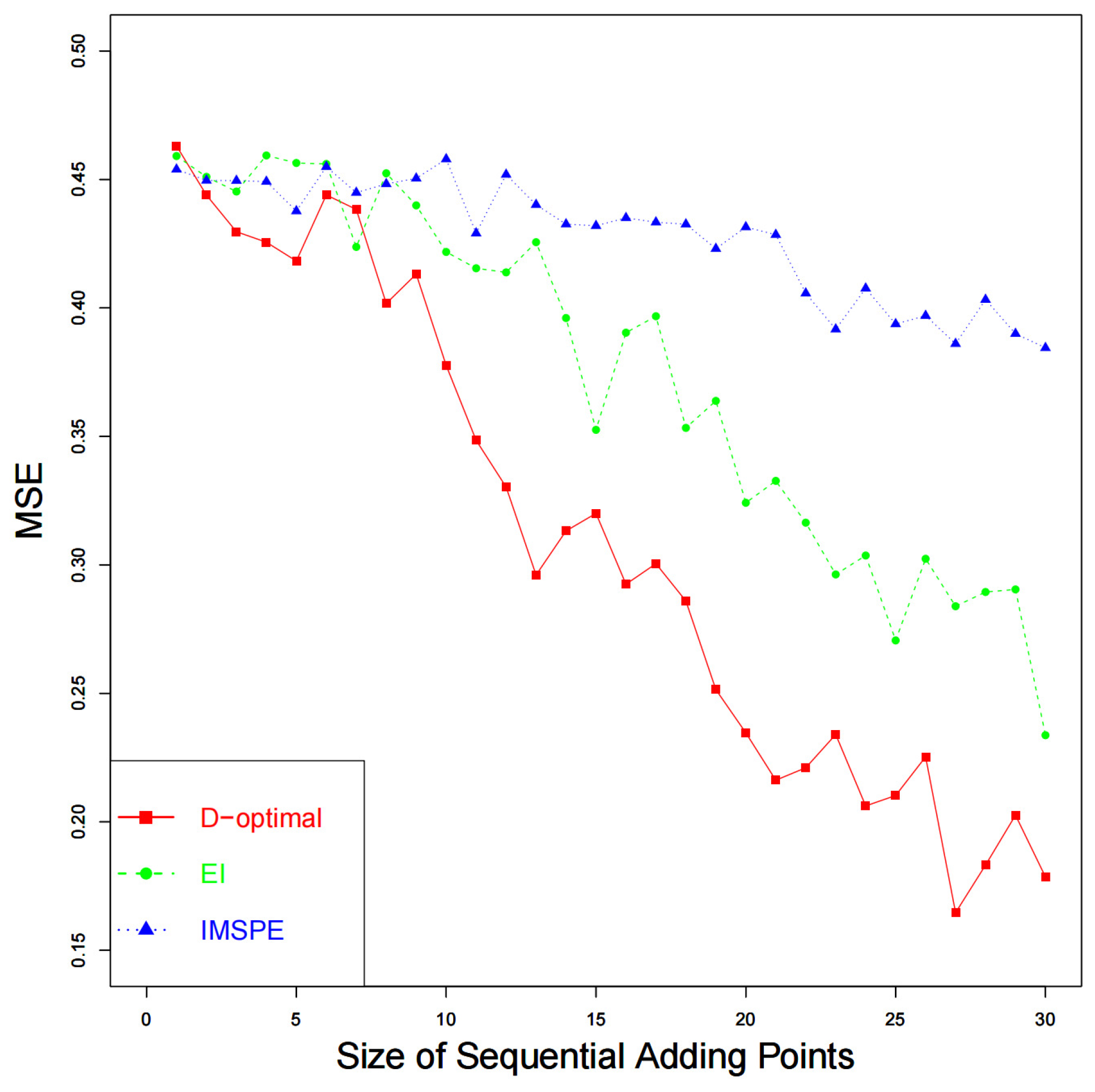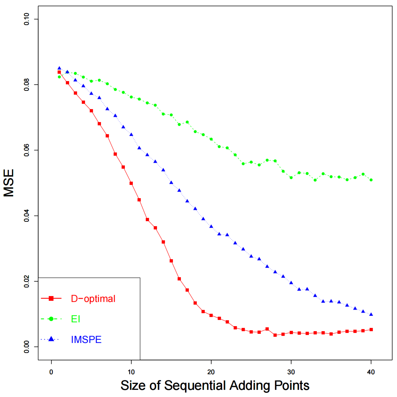An MmLHD in $[-5,5]\times [0,3]$ with 10 points is generated for the initial computer experiment design, i.e., $n=10$, and the $N=30$ points are to be added sequentially according to Algorithm 1. A total of 100 simulations are performed to calculate the metrics of performance. 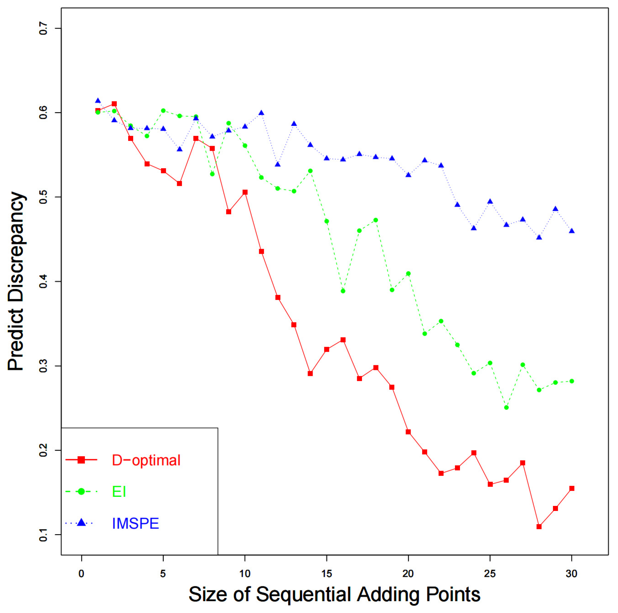The results of $MS{E}_l$ are shown in Figure 1. As the increase in computer experimental points sequentially, the calibration parameter approaches the best value, and the proposed method outperforms the other two designs. 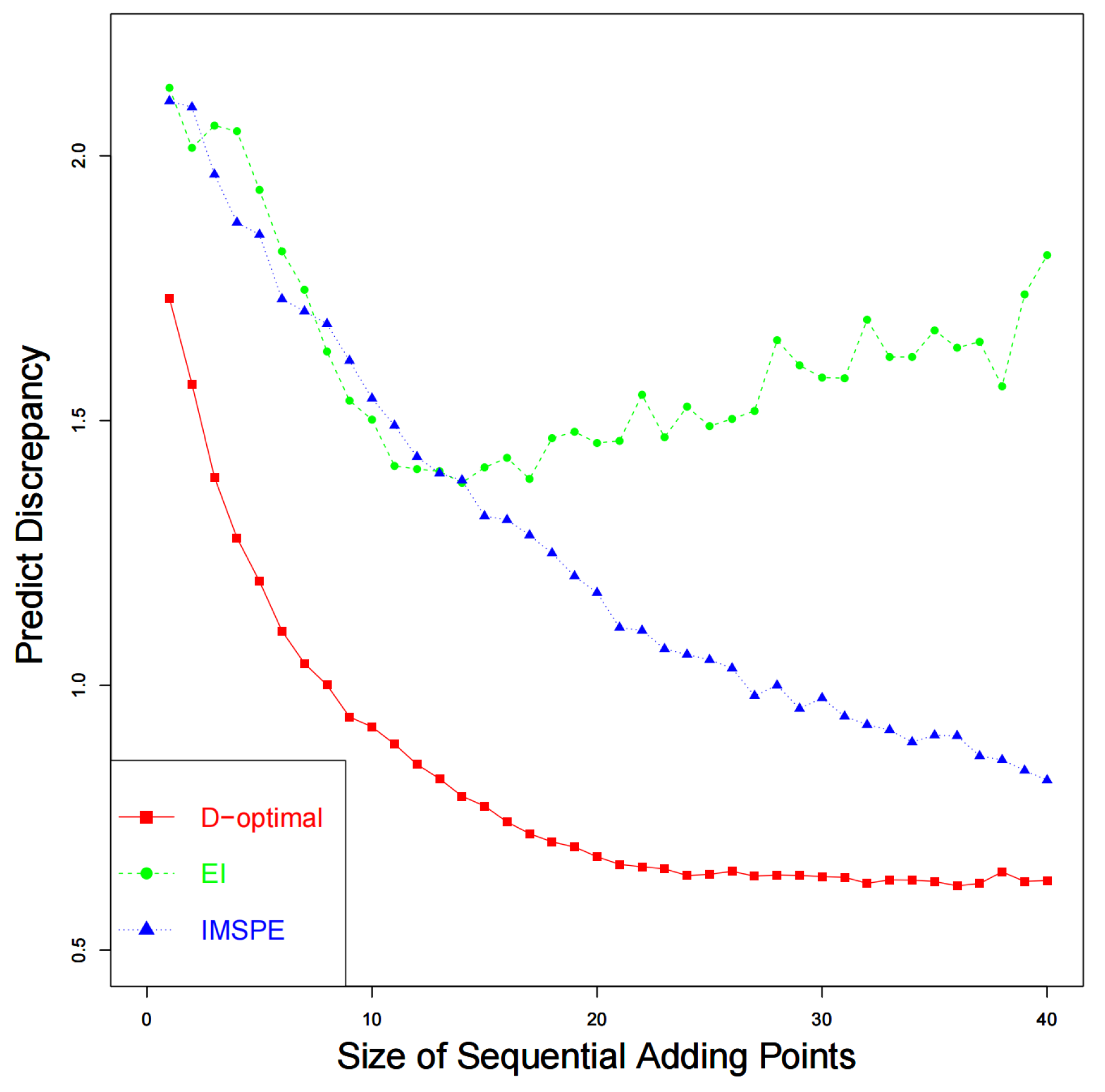The results of $MP{D}_l$ are shown in Figure 2, which shares a similar trend with $MS{E}_l$. 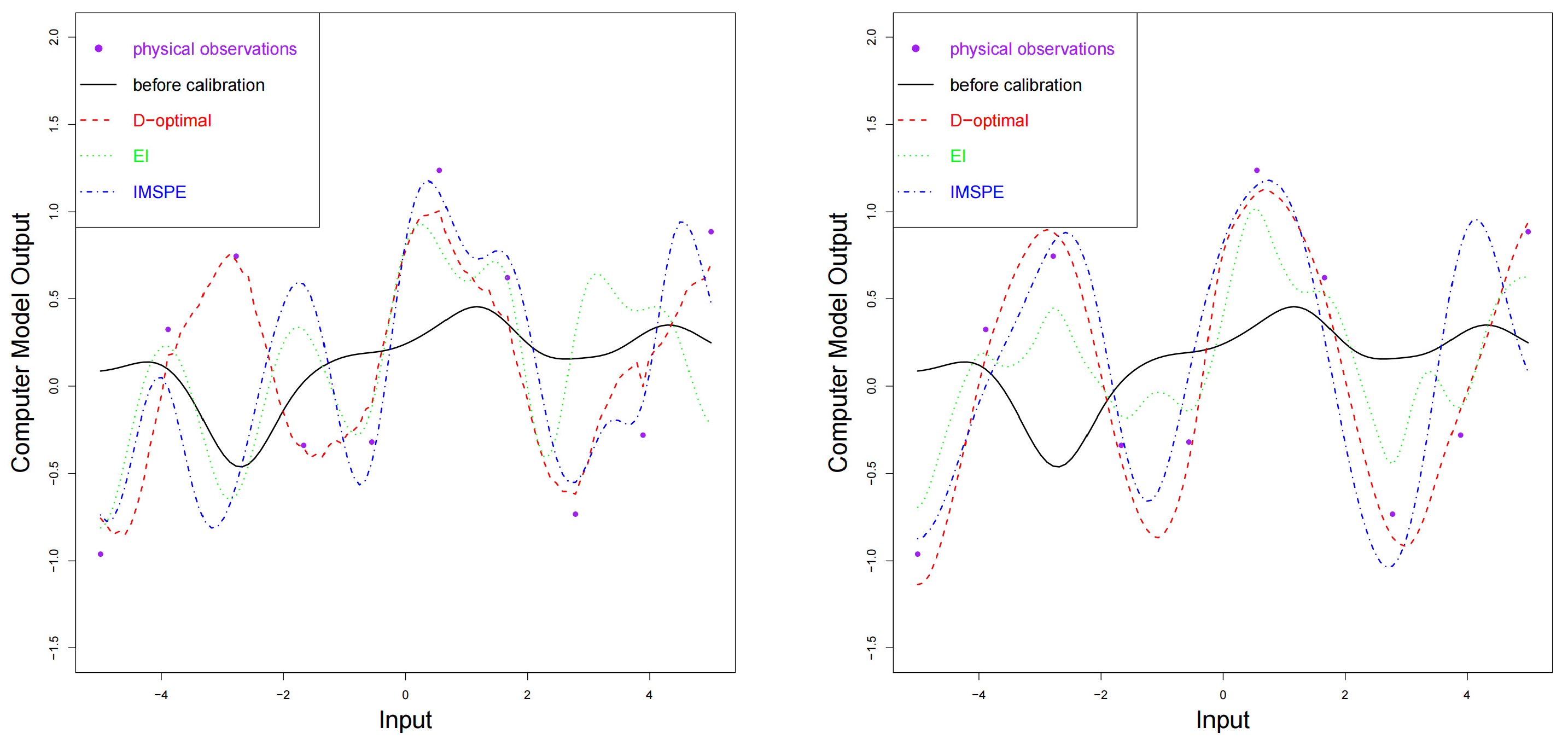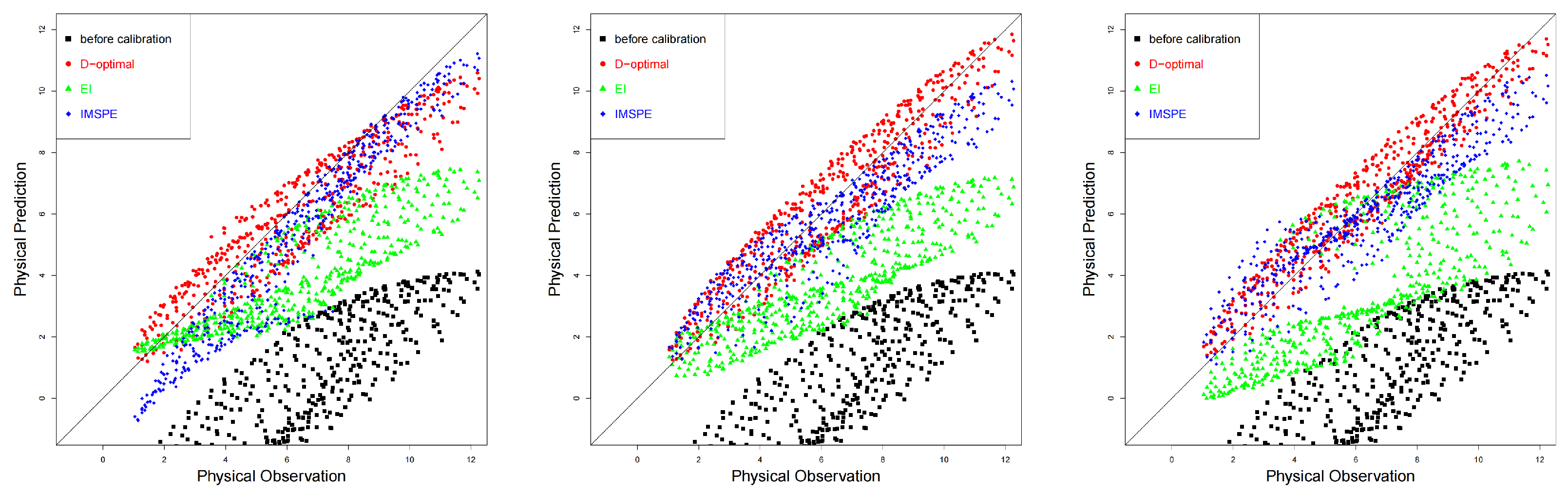The comparison between the original computer model and the calibrated computer model is shown in Figure 3. We can see that the calibrated computer models are closer to the physical observations. As the number of sequential computer experiments increases, the differences between the computer model and physical observations decrease, and the proposed method performs better than the other two designs.

Figure 1. $MS{E}_l$ of $\theta$ obtained using the proposed sequential D-optimal method, EI method, and IMSPE method by sequentially adding computer experiment points.

Figure 2. $MP{D}_l$ obtained using the proposed sequential D-optimal method, EI method, and IMSPE method.

Figure 3. Model outputs before and after calibration through the proposed sequential D-optimal method, EI method, and IMSPE method, compared with the physical observations. The left and right panels show the results obtained by sequentially adding 14 and 30 points, respectively.

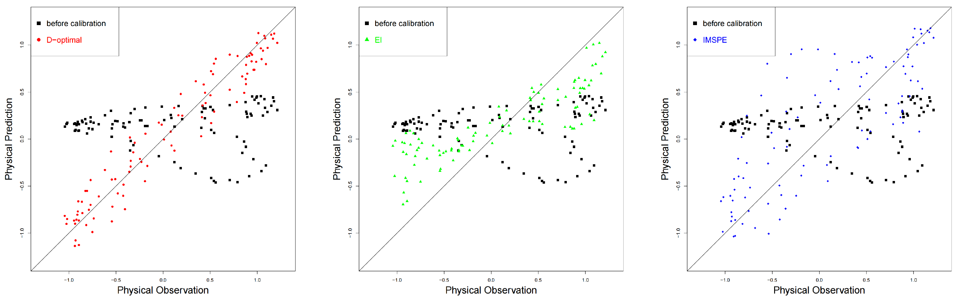
The results of $MSP{E}_l$ are summarized in Table 1, which also shares a similar trend with $MP{D}_l$ and $MS{E}_l$. The performance of prediction by combining calibrated computer models and discrepancy function is shown in Figure 4. In Figure 4, the predictions by using our method approximate the physical observations best.

Table 1. The results about $MSP{E}_l$.

Number of Sequential Points	Before Calibration	D-Optimal	EI	IMSPE
14	0.5892141	0.1429672	0.5869769	0.4524031
30	0.5892141	0.03625579	0.218899	0.2244712

Figure 4. Physical predictions before and after calibration with the proposed sequential D-optimal method, EI method, and IMSPE method with 30 sequential computer experimental points.

4.2. Case Study II

In this section, another example which includes three calibration parameters and two control variables and is given in [28] is considered. In this case study, a discrepancy between computer model outputs and physical outputs is also regarding. The physical process is described as

$$\begin{array}{c}\hfill y^p(\mathit{x})=7{[sin(2\pi {\theta }_1-\pi )]}^2+2{(2\pi {\theta }_2-\pi )}^{2}sin(2\pi x_1-\pi )+6{\theta }_3(x_2-0.5)+\delta (\mathit{x})+ϵ,\end{array}$$

where, $ϵ\sim N(0,0.01)$, $\delta (\mathit{x})=cos(2\pi x_1-\pi )+2({x_2}^2-x_2+1/6)$, $\mathit{x}=(x_1,x_2)\in {[0,1]}^2$, $\mathit{\theta }=({\theta }_1,{\theta }_2,{\theta }_3)\in [0,0.25]\times [0,0.5]\times [0,1]$. The best value of the calibration parameter is ${\mathit{\theta }}^{*}=(0.2,0.3,0.8)$. Assume that the expectation of $y^c(\mathit{x},\mathit{\theta })$ is $\mathit{\beta }$, and the correlation function of $y^c(\mathit{x},\mathit{\theta })$ is Gaussian. The expectation of $\delta (\mathit{x})$ is set to be zero, and the correlation function of $\delta (\mathit{x})$ is also assumed to be Gaussian. Let the prior for ${\theta }_1$, ${\theta }_2$, and ${\theta }_3$ be $U(0,0.25)$, $U(0,0.5)$, and $U(0,1)$, respectively. A total of 500 simulations are performed to assess the performances of the sequential designs. A design with 10 points are employed for physical experiments, and a MmLHD with $n=20$ points over ${[-1,1]}^3\times [0,0.25]\times [0,0.5]$ is utilized as the initial design for computer experiments. In this case, the number of sequential points is set to be $N=40$. The results of $MS{E}_l$ are drawn in Figure 5. As the size of sequential experiment points increases, the calibration parameter approaches the best value. The proposed method has smaller MSEs than the other two methods, which means the proposed method performs better. Figure 6 shows the results of $MP{D}_l$, which also demonstrate the effectiveness of the proposed design for calibration.

Figure 5. $MS{E}_l$ of $\mathit{\theta }$ obtained using the proposed sequential D-optimal method, EI method, and IMSPE method by sequentially adding computer experiment points.

Figure 6. $MP{D}_l$ obtained using the proposed sequential D-optimal method, EI method, and IMSPE method.

The simulation results in Figure 1 and Figure 5 show that, regardless of whether the discrepancy function exists or not, with the increase in sequential points, the estimate of calibration parameters gradually approaches its best value, indicating that the estimation of calibration parameters converges. However, the strict mathematical proof of this conclusion is a complicated problem, which cannot be solved in this paper and will be paid attention to in a future study.

From Figure 6, we can easily find out that when 20 points are sequentially added, the discrepancy tends to be stable. As shown in Figure 7, the physical prediction combining discrepancy and calibrated computer model by utilizing the proposed sequential D-optimal method is the closest to the physical observations, followed by the IMSPE method and EI method. The results regarding the MSPE are presented in Table 2, which shares similar conclusions as those in the case study I.

Figure 7. Physical predictions before and after calibration using the D-optimal method, EI method, and IMSPE method. The left, middle, and right panels show the results of sequentially adding 20, 25, and 40 points, respectively.

Table 2. The results for $MSP{E}_l$.

Number of Sequential Points	Before Calibration	D-Optimal	EI	IMSPE
20 points	39.68042	1.187998	8.09301	1.808175
25 points	39.68042	0.7716595	8.97966	1.48396
40 points	39.68042	0.5952004	10.52075	1.336039

4.3. Real Data Analysis

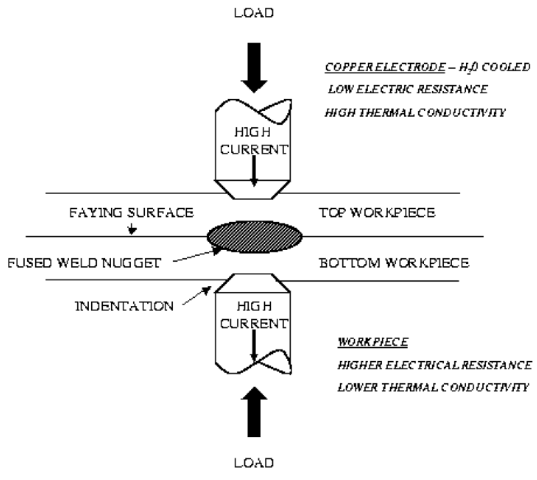
In this section, a real data example with three control inputs and one calibration input is considered, which is presented in [8]. Figure 8 shows a concise description of the resistance spot welding process. Two metal sheets of a particular thickness (thickness) are compressed through two electrodes under a specifically applied load (load). A direct current of a certain magnitude (current) passes through the sheets via the two electrodes, and the heat produced by the current flow causes the welding surfaces to melt. After cooling, a weld nugget with a specific dimension (diameter) is formed, which is of particular interest. In this manner, the two metal plates are welded.

Figure 8. Schematic of the spot-welding process.

The resistance at the contact surface is particularly critical in determining the magnitude of heat generated. Because the contact resistance at the contact surface is not well understood as a function of temperature, the calibration parameter is specified and adjusted based on the field data. The effect of this calibration parameter on the behavior of the model is a focus in this case. Ref. [8] comprehensively described the inputs for this example. According to the evaluation of the model developer, the verification experiment focuses on three control inputs (thickness, load, and current). Table 3 lists the control and calibration inputs and the corresponding intervals.

Table 3. Control inputs and calibration input.

Load (kN)	Thickness (mm)	Current (kA)	Resistance
$[4.0,5.3]$	1 or 2	$[21,26]$ for thickness 1	$[0.8,8]$
		$[24,29]$ for thickness 2

A constant mean $\beta$ and the product-form exponential correlation function are considered as the prior for $y^c(\mathit{x},\theta )$. As (2) shows, a zero mean and the Gaussian correlation function are considered as the prior for $\delta (\mathit{x})$, and more details can be found in [2,6,28,29], etc. We randomly choose 10 physical experiments from the non-replicated 12 physical experiments. An initial computer design with 20 points is generated and the corresponding outputs are simulated according to [8]. $N=40$ points are added sequentially according to Algorithm 1. The results about the MSPE are summarized in Table 4, which illustrates the superior of the new proposed method due to the smaller MSPE values.

Table 4. MSPE before and after calibration.

Number of Sequential Points	Before Calibration	D-Optimal	EI	IMSPE
20 points	1.384987	0.432674	0.9045898	0.4400638
25 points	1.384987	0.3496204	0.8424071	0.3827046
40 points	1.384987	0.3328246	1.041911	0.3804081

5. Conclusions and Remark

In order to reduce the cost of physical experiments, mathematical models or computer models are utilized to approximate the real physical process. However, the computer models’ fidelity to physical process depends on the physical unobservable calibration parameters. This paper proposed a D-optimal design to augment computer experiments sequentially by regarding the Kennedy and O’Hagan model. By using the D-optimal criterion, computer design points are selected sequentially to gather more comprehensive information to reduce the uncertainty about the estimate of the calibration parameter. Then, the computer model can mimic the real physical process well with the tuned calibration parameter. Simulation studies are made to assess the performance of the newly proposed method compared with EI and IMSPE methods. The results show that the newly proposed method outperforms the other two methods in terms of $MSE$, $MPD$, and $MSPE$. An analysis based on the real data introduced in [8] also demonstrates the superior performance of the new method.