Modelling Asymmetric Data by Using the Log-Gamma-Normal Regression Model

Abstract

In this paper, we propose a linear regression model in which the error term follows a log-gamma-normal (LGN) distribution. The assumption of LGN distribution gives flexibility to accommodate skew forms to the left and to the right. Kurtosis greater or smaller than the normal model can also be accommodated. The regression model for censored asymmetric data is also considered (censored LGN model). Parameter estimation is implemented using the maximum likelihood approach and a small simulation study is conducted to evaluate parameter recovery. The main conclusion is that the approach is very much satisfactory for moderate and large sample sizes. Results for two applications of the proposed model to real datasets are provided for illustrative purposes.

1. Introduction

Regression models are one of the main statistical techniques frequently used in data analysis in any area of knowledge, especially when there is interest in studying the relationship between a dependent variable (response) and two or more independent (explanatory) variables. In this sense, a regression model with a response variable following a normal distribution is perhaps best known in the literature, and could be considered one of the most widely used; however, the assumption of normality may not be adequate in the dataset under analysis, since these may present degrees of skewness or kurtosis that are not within the range covered by the normal model. Consequently, inferences made from the fitted model may not have statistical validity, and erroneous conclusions may be reached. A solution to the problem of the assumption of normality of the variable of interest is the use of transformations, although it is well known that this solution makes it difficult to interpret results since data are not in the original measurement scale. As an alternative to this issue, many authors have introduced new family distributions that are capable of capturing degrees of skewness and kurtosis greater than those that the normal distribution can capture.

One of the most important works in the context of data with a high degree of asymmetry is Azzalini [1], which is known in the statistical literature as the skew-normal (SN) model. The main characteristic of the SN model is its ability to fit degrees of asymmetry (on the left and right) greater than those of the normal model; however, it is not the best model in terms of capturing high degrees of kurtosis. Relating to the latter, the power-normal (PN) model introduced by Durrans [2] has the particularity of fitting data with a higher degree of kurtosis than the normal and SN model but with less range of asymmetry. The SN and PN models have been studied extensively by many authors, and different extensions of this model have been considered. In Gupta and Gupta [3] for example, the authors showed the existing practical problems when the asymmetry parameter of the SN model is estimated, and they proposed an alternative model named the PN model. The authors also investigated the closeness between the proposed model and the SN model. In Pewsey et al. [4], the authors presented the general results of the likelihood-based inference for the family of power distributions, with particular emphasis on the case of the PN model, complementing the work of Gupta and Gupta [3]. In Martínez-Flórez et al. [5], the authors introduced a new model that generalized both the SN model by Azzalini [1] and the PN model by Durrans [2]. The new model, which is called power-skew-normal (PSN), has the particularity of fitting data with degrees of asymmetry greater than those of the SN model, and is also capable of capturing degrees of kurtosis greater than those of the PN model. Furthermore, the authors showed that the information matrix of the new model is non-singular, which permits carrying out hypothesis tests on the asymmetry parameters based on likelihood-ratio statistics. On the other hand, Martínez-Flórez et al. [6] generalized the log-normal (LN) model from the SN and PN models. In addition, these new proposals contain the LN model as a particular case, and they are more flexible regarding skewness and kurtosis to fit positive data.

Alternatives for fitting asymmetric data with a high degree of kurtosis were reported by other authors such as Tovar-Falón et al. [7], who introduced a new model that generalizes the skew-t model of Azzalini and Capitanio [8] and power-t of Zhao and Kim [9]. Here, the inference was carried out from a classical perspective using the maximum likelihood method. This new model also has, as particular cases, the PSN, SN, PN, Student-t and normal models. In Tung et al. [10], the authors considered a mixture class of log-F distributions to characterize asymmetric distributions by integrating it into a pH acceleration model. The authors studied the impact of the new model in the presence of misspecification of particle size distribution.

Models for asymmetric data with high degrees of skewness and kurtosis, and presenting more than one mode and censored data, were also considered. More details about these topics can be found in Martínez-Flórez et al. [11] and Martínez-Flórez et al. [12], respectively. In addition, all the aforementioned models are easily extensible to the situations of regression models, including cases in which the data show censoring in some value; see Sahu et al. [13], Martínez-Flórez et al. [14].

In Amini et al. [15], the authors introduced a new family of distributions useful for modelling asymmetric data. This new family of continuous distributions is generated by a distribution F and two positive real parameters $\delta$ and $\gamma$, which control the skewness and tail weight of the distribution. The probability density function (PDF) of this family is given by

$$g(x;\delta ,\gamma )=\frac{{\gamma }^{\delta }}{\mathrm{\Gamma }\left(\delta \right)}{\left[-lnF\left(x\right)\right]}^{\delta -1}{\left[F\left(x\right)\right]}^{\gamma -1}f\left(x\right),$$

(1)

where $\delta ,\gamma \in {\mathbb{R}}^{+}$ and $\mathrm{\Gamma }(·)$ is the complete gamma function, $F(·)$ is the cumulative distribution function (CDF) of X, and $f(·)$ is the associated PDF. In this work, the authors studied the main properties of the distribution and addressed the estimation process of the unknown parameters of the model using the likelihood approach.

From the $F\left(x\right)$ generator, the authors studied some particular properties of the family, among which are the exponential, Weibull, power, Pareto, extreme value and Gumbel distributions. If $\delta =1$ and $F(·)=\mathrm{\Phi }(·)$ and $f(·)=\varphi (·)$ in model (1), i.e., the CDF and PDF of the standard normal distribution, respectively, the model in (1) is reduced to the PN model by Durrans [2]. Hence, the model in (1) is an extension of the PN model. In Cordeiro et al. [16], the authors studied in detail the properties of the log-gamma-generated family of distributions introduced by Amini et al. [15] and presented some applications of this family. Other particular cases of the model introduced by Amini et al. [15] correspond to the generalized gamma and log-gamma distributions, which have been extensively studied by many authors; see Prentice [17], Lawless [18], Young and Bakir [19], Ortega et al. [20, 21] among others.

The main goal of this article is to focus on the study of the regression model under the assumption that the errors follow a log-gamma-normal (LGN) distribution, which is obtained by taking $F\left(x\right)=\mathrm{\Phi }\left(x\right)$ and $f\left(x\right)=\varphi \left(x\right)$ in model (1). We also consider the case of the regression model for censored data, and we conduce the parameter estimation using the maximum likelihood approach and its large sample properties.

Although there are many works in the literature related to the generalized log-gamma distribution, our proposal is based on the family of distributions presented by Amini et al. [15], which is known in the literature as log-gamma-generated. For the case of this family, we focus on the case in which the generating function is the normal distribution and the distribution called log-gamma-normal is obtained, and this distribution does not correspond to the distributions previously mentioned. In our proposal, we change the assumption that the errors in the multiple linear regression model follow a normal distribution to that of errors with a log-gamma-normal distribution. It is also important to note that the generalized log-gamma and log-gamma distributions are also particular cases of the family introduced by Amini et al. [15] (assuming a gamma distribution instead of the standard normal distribution), but in our proposal we do not consider these cases.

In addition to carrying out the estimation process of the parameters in the model, we present two applications using real datasets. The first dataset was previously analyzed by Zhang and Davidian [22], and the second dataset is related to a study on the abundance of beryllium scaled to the Sun’s abundance. For the particular case of these datasets, the model fits well, and therefore we can conclude that, apart from the existence of statistical literature for the analysis of asymmetric data, our proposal is a viable alternative that competes with existing models. The main contribution of this model is that the trend of the dataset under examination is better explained using a model with log-gamma type errors instead of one with asymmetric errors using another distribution.

The article is organized as follows. In Section 2, we define the family of LGN distributions and discuss some of its properties. In Section 3, the LGN regression model is defined, and its properties studied. The inference is implemented using the maximum likelihood approach. The censored LGN model for dealing with censored data by maximum likelihood estimation is discussed in Section 4. The results of a small-scale simulation study reveal the good performance of the estimation approach in Section 5. In Section 6, two real data applications are considered, revealing that the datasets in question are better fitted by LGN model than PN and models.

2. Log-Gamma-Normal Distribution

In this section, we define the LGN model, which is obtained from the family given in (1) by taking the CDF of the standard normal distribution, and we study some basic properties.

Definition 1.

The random variable X is said to have a LGN distribution, if X has PDF given by

$$f_{LGN}(x;\delta ,\gamma )=\frac{{\gamma }^{\delta }}{\mathrm{\Gamma }\left(\delta \right)}{\left[-ln\mathrm{\Phi }\left(x\right)\right]}^{\delta -1}{\left[\mathrm{\Phi }\left(x\right)\right]}^{\gamma -1}\varphi \left(x\right),x\in \mathbb{R},$$

(2)

where $\delta ,\gamma \in {\mathbb{R}}^{+}$, $\mathrm{\Gamma }\left(a\right)={\int }_0^{\infty }{u}^{a-1}{e}^{-u}du$ is the gamma function, and the functions $\varphi (·)$ and $\mathrm{\Phi }(·)$ are the PDF and CDF of the standard normal distribution, respectively.

A random variable with LGN distribution is shortly denoted by $X\sim \mathrm{LGN}(\delta ,\gamma )$. One can note that the function (2) is a proper PDF since $f_{LGN}(x;\delta ,\gamma )\ge 0$ for all $x\in \mathbb{R}$ and $\delta ,\gamma \in {\mathbb{R}}^{+}$. Thus, letting $y=-ln\mathrm{\Phi }\left(x\right)$, it follows that

$${\int }_{\mathbb{R}}\frac{{\gamma }^{\delta }}{\mathrm{\Gamma }\left(\delta \right)}{\left[-ln\mathrm{\Phi }\left(x\right)\right]}^{\delta -1}{\left[\mathrm{\Phi }\left(x\right)\right]}^{\gamma -1}\varphi \left(x\right)dx={\int }_0^{+\infty }\frac{{\gamma }^{\delta }}{\mathrm{\Gamma }\left(\delta \right)}{y}^{\delta -1}{e}^{-\gamma y}dy=1.$$

Figure 1 depicts some shapes of LGN distribution for some selected values of the parameters $\delta$ and $\gamma$. It can be seen that the parameters $\delta$ and $\gamma$ affect both the skewness and kurtosis of the model, and hence, the LGN distribution is more flexible for fitting data that may be skewed as well as having thinner or thicker tails than the normal, SN and PN distributions.

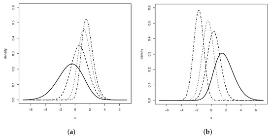
Figure 1. PDF of the LGN distribution: (a) $\delta =0.6$ and $\gamma =0.30$ (dotted line), 0.60 (dashed line), 1.0 (dotted–dashed line), 3.0 (long dashed line) and 6.0 (solid line). (b) $\gamma =1.5$ and $\delta =0.30$ (dotted line), 0.60 (dashed line), 1.0 (dotted–dashed line), 2.0 (long dashed line) and 5.0 (solid line).

The LGN distribution reduces to some specific distributions as special cases for specified values of the parameters $\delta$ and $\gamma$; some of them are available in the literature and have been widely studied.

Proposition 1.

Let $X\sim LGN(\delta ,\gamma )$

(i)

if$\delta =\gamma =1$, then$X\sim N(0,1)$,

(ii)

if$\delta =1$, then$X\sim PN\left(\gamma \right)$,

(iii)

if$\delta =1$and$\gamma =2$, then$X\sim SN\left(1\right)$.

Proof. 

Demonstration of (i)–(iii) is immediate from the definition of LGN distribution. □

2.1. Moments

Measures of skewness and kurtosis can be given from the moments of the LGN distribution. The following proposition gives an expression of the rth moment of the random variable $X\sim \mathrm{LGN}(\delta ,\gamma )$ which does not have a closed form.

Proposition 2.

Let$X\sim LGN(\delta ,\gamma )$then

$$\mathbb{E}\left[X^k\right]=\mathbb{E}\left[{\left({\mathrm{\Phi }}^{-1}\left(e^{-W}\right)\right)}^k\right],\mathrm{for}k=1,\dots ,n,$$

(3)

where${\mathrm{\Phi }}^{-1}(·)$is the inverse of the CDF$\mathrm{\Phi }(·)$and the random variable W follows a gamma distribution with parameters δ and γ.

Proof. 

We have by definition that

$$\mathbb{E}\left[X^k\right]={\int }_{\mathbb{R}}{x}^k\frac{{\gamma }^{\delta }}{\mathrm{\Gamma }\left(\delta \right)}{\left[-ln\mathrm{\Phi }\left(x\right)\right]}^{\delta -1}{\left[\mathrm{\Phi }\left(x\right)\right]}^{\gamma -1}\varphi \left(x\right)dx.$$

Letting $W=-ln\mathrm{\Phi }\left(X\right)$, then $X={\mathrm{\Phi }}^{-1}\left(e^{-W}\right)$, it follows that

$$\mathbb{E}\left[X^k\right]={\int }_0^{+\infty }{\left({\mathrm{\Phi }}^{-1}\left(e^{-w}\right)\right)}^k\frac{{\gamma }^{\delta }}{\mathrm{\Gamma }\left(\delta \right)}{w}^{\delta -1}{e}^{-\gamma w}dw,$$

which is the expected value of the function ${\left[{\mathrm{\Phi }}^{-1}\left(e^{-W}\right)\right]}^k$, where W follows a $\mathrm{Gamma}(\delta ,\gamma )$ distribution. □

Based on moments (3), one can obtain the skewness $\left(\sqrt{{\beta }_1}\right)$ and the kurtosis $\left({\beta }_2\right)$ coefficients of the LGN model using the following expressions

$$\sqrt{{\beta }_1}=\frac{{\mu }_3-3{\mu }_1{\mu }_2+2{\mu }_1^3}{{({\mu }_2-{\mu }_1^2)}^{3/2}},$$

and

$${\beta }_2=\frac{{\mu }_4-4{\mu }_1{\mu }_3+6{\mu }_2{\mu }_1^2-3{\mu }_1^4}{{({\mu }_2-{\mu }_1^2)}^2}$$

respectively, where ${\mu }_k=\mathbb{E}\left[X^k\right]$ for $k=1,\dots ,4$. The skewness and kurtosis coefficients for values of $\delta$ and $\gamma$ ranging between 0.1 and 200 were calculated using numerical integration with an integrate function of R Development Core Team [23] for LGN model. It was found that $\sqrt{{\beta }_1}\in [-1.0190,1.0143]$ and ${\beta }_2\in [1.7170,4.9356]$. The given intervals contain the corresponding intervals of skewness and kurtosis coefficients of the SN model, which are $(-0.9953,0.9953)$ and $[3.0000,3.8692)$, respectively, and the PN model, which are $[-0.6115,0.9007]$ and $[1.7170,4.3556]$, respectively. More details can be found in Pewsey et al. [4]. The previous results illustrate the fact that the LGN model contains models with greater (and smaller) asymmetry degree than both the SN and PN models.

2.2. Distribution Function

In this section, we present the explicit formula for the CDF of LGN distribution.

Proposition 3.

Let$X\sim LGN(\delta ,\gamma )$, then

$$F_{LGN}\left(x\right)=\frac{\mathrm{\Gamma }\left(\delta ,-\gamma ln\mathrm{\Phi }\left(x\right)\right)}{\mathrm{\Gamma }\left(\delta \right)},$$

(4)

where$\mathrm{\Gamma }\left(a\right)={\int }_0^{\infty }{u}^{a-1}{e}^{-u}du$is the gamma function and$\mathrm{\Gamma }\left(a,x\right)={\int }_x^{\infty }{u}^{a-1}{e}^{-u}dx$is the upper incomplete gamma function.

Proof. 

The CDF of the LGN distribution is obtained as follows:

$$\begin{array}{cc}\hfill F_{LGN}\left(x\right)& ={\int }_{-\infty }^x{f}_{LGN}\left(t\right)dt\hfill \\ \hfill & ={\int }_{-\infty }^x\frac{{\gamma }^{\delta }}{\mathrm{\Gamma }\left(\delta \right)}{\left[-ln\mathrm{\Phi }\left(t\right)\right]}^{\delta -1}{\left[\mathrm{\Phi }\left(t\right)\right]}^{\gamma -1}\varphi \left(t\right)dt\hfill \\ \hfill & =-{\int }_{+\infty }^{-ln\mathrm{\Phi }\left(x\right)}\frac{{\gamma }^{\delta }}{\mathrm{\Gamma }\left(\delta \right)}{s}^{\delta -1}{e}^{-\gamma s}ds;\mathrm{by}s=-ln\mathrm{\Phi }\left(t\right)\hfill \\ \hfill & ={\int }_{-ln\mathrm{\Phi }\left(x\right)}^{+\infty }\frac{{\gamma }^{\delta }}{\mathrm{\Gamma }\left(\delta \right)}{s}^{\delta -1}{e}^{-\gamma s}ds\hfill \\ \hfill & =\frac{\mathrm{\Gamma }\left(\delta ,-\gamma ln\mathrm{\Phi }\left(x\right)\right)}{\mathrm{\Gamma }\left(\delta \right)}\hfill \end{array}$$

□

It can be shown that (see Cordeiro et al. [16]) for the density function given in (2), the quantile function is given by:

$$Q\left(u\right)={\mathrm{\Phi }}^{-1}\left(exp\left\{-{\gamma }^{-1}{Q}^{-1}(\delta ,u)\right\}\right),$$

where $Q^{-1}(\delta ,u)$ is the inverse function of $Q(\delta ,u)=\mathrm{\Gamma }(\delta ,u)/\left(\mathrm{\Gamma }\right(\delta \left)\right)$.

The inversion method can be used to generate a random variable with LGN distribution. Thus, let $\delta ,\gamma \in {\mathbb{R}}^{+}$ and U be a random variable with uniform distribution, namely $U\sim \mathrm{U}(0,1)$. Then, the random variable X with distribution $\mathrm{LGN}(\delta ,\gamma )$ can be obtained by letting

$$X={\mathrm{\Phi }}^{-1}\left(e^{-F^{-1}\left(1-U,\delta ,\gamma \right)}\right),$$

where ${\mathrm{\Phi }}^{-1}(·)$ and $F^{-1}(·,\delta ,\gamma )$ are the inverses of the CDF of the normal and gamma distributions, respectively. The survival and hazard functions for the LGN distribution can be obtained from (2) and (4), and they are given by

$$S\left(t\right)=\mathrm{\Gamma }\left(-ln\mathrm{\Phi }\left(t\right);\delta ,\gamma \right),$$

and

$$r\left(t\right)=\frac{\frac{{\gamma }^{\delta }}{\mathrm{\Gamma }\left(\delta \right)}{\left[-ln\mathrm{\Phi }\left(t\right)\right]}^{\delta -1}{\left[\mathrm{\Phi }\left(t\right)\right]}^{\gamma -1}\varphi \left(t\right)}{\mathrm{\Gamma }\left(-ln\mathrm{\Phi }\left(t\right),\delta ,\gamma \right)},$$

respectively.

2.3. Location-Scale Extension

Let $X\sim LGN(\delta ,\gamma )$. The location-scale extension of the random variable X is defined using the transformation $Y=\xi +\sigma X$, where $\xi \in \mathbb{R}$ and $\sigma \in {\mathbb{R}}^{+}$. The corresponding PDF of Y is given by

$$\begin{array}{cc}\hfill f_{LGN}(y;\xi ,\sigma ,\delta ,\gamma )& =\frac{{\gamma }^{\delta }}{\sigma \mathrm{\Gamma }\left(\delta \right)}{\left[-ln\mathrm{\Phi }\left(\frac{y-\xi }{\sigma }\right)\right]}^{\delta -1}{\left[\mathrm{\Phi }\left(\frac{y-\xi }{\sigma }\right)\right]}^{\gamma -1}\varphi \left(\frac{y-\xi }{\sigma }\right),\hfill \end{array}$$

(5)

where $\xi$ is a location parameter and $\sigma$ is a scale parameter. The random variable Y that has a distribution with density function given in Equation (5) is denoted as $Y\sim LGN(\xi ,\sigma ,\delta ,\gamma )$.

The previous representation of location scale can be extended to the case where response variable depends on regressor variables, say $Z_1,\dots ,Z_p$, through the relationship ${\xi }_i={\mathbf{z}}_i^{\top }\beta$; where $\beta ={({\beta }_0,{\beta }_1,\dots ,{\beta }_p)}^{\top }$ is an unknown vector of regression coefficients and $\mathbf{z}={(1,z_1,\dots ,z_p)}^{\top }$ is a vector of known regressors correlated with the response vector.

The rth moment of a variable $Y\sim \mathrm{LGN}(\xi ,\sigma ,\delta ,\gamma )$ can be obtained using the formula

$$\mathbb{E}\left[Y^r\right]=\sum _{l=0}^r\left(\genfrac{}{}{0pt}{}{r}{l}\right){\xi }^l{\sigma }^{r-l}\mathbb{E}\left[X^{r-l}\right],r=1,\dots ,$$

where $X\sim \mathrm{LGN}(\delta ,\gamma )$.

Proof. 

Let $X\sim \mathrm{LGN}(\delta ,\gamma )$, then, for $Y=\xi +\sigma X$ and $r=1,\dots$ it has

$$\begin{array}{cc}\hfill \mathbb{E}\left[Y^r\right]& =\mathbb{E}\left[{(\xi +\sigma X)}^r\right]\hfill \\ \hfill & =\mathbb{E}\left[\sum _{l=0}^r\left(\genfrac{}{}{0pt}{}{r}{l}\right){\xi }^l{\left(\sigma X\right)}^{r-l}\right]\hfill \\ \hfill & =\sum _{l=0}^r\left(\genfrac{}{}{0pt}{}{r}{l}\right){\xi }^l{\sigma }^{r-l}\mathbb{E}\left[X^{r-l}\right].\hfill \end{array}$$

In the second line, the binomial theorem is used. □

3. Log-Gamma-Normal Regression Model

Regression models have been a statistical technique widely used in many areas of knowledge to explain the behavior of a response variable, say Y, as a function of other variables called regressors, say $Z_1,\dots ,Z_p$, and a vector of unknown parameters called regression coefficients denoted by $\mathbf{\beta }$. Specifically, for a random sample of n individuals indexed by $i=1,\dots ,n$, we have

$$y_i={\mathbf{z}}_i^{\top }\mathbf{\beta }+{\epsilon }_i\mathrm{for}i=1,2,\dots ,n;$$

(6)

where ${\epsilon }_i$ is a random variable (random error) with certain PDF, the most common being the normal distribution assumption, i.e., ${\epsilon }_i\sim N(0,{\sigma }^2)$. Given the multiple departures from the normality assumption and the actual behavior of the random variable ${\epsilon }_i$, this assumption has been replaced in numerous instances by other more realistic ones, usually looking for distributions to fit data with higher or lower skewness and/or kurtosis than that allowed by the normal distribution. Notable inferential mistakes are made (invalid results) when we work under the normal assumption and this assumption is not true. In some cases, a simple transformation helps to solve this problem, but this strategy typically has problems of interpretability of the results or the coefficients of the model.

Now, we change the normal assumption using the LGN assumption in the random error term ${\epsilon }_i$, so we suppose that ${\epsilon }_i\sim \mathrm{LGN}(0,\sigma ,\delta ,\gamma )$ and this leads to $Y_i\sim \mathrm{LGN}({\mathbf{z}}_i^{\top }\mathbf{\beta },\sigma ,\delta ,\gamma )$ for $i=1,\dots ,n$. The case $\delta =\gamma =1$ follows the ordinary normal regression model. Using the least squares method, we obtain the estimators $\tilde{\mathbf{\beta }}={\left({\mathbf{z}}^{\top }\mathbf{z}\right)}^{-1}{\mathbf{z}}^{\top }\mathbf{y}$, which are not unbiased for the parameters of the regression coefficients but the correction ${\tilde{\beta }}_0^{*}={\tilde{\beta }}_0+\widehat{\mathbb{E}}\left[\epsilon \right]$, where the last term represents the estimated expected value of the random variable $\epsilon$, such that we can obtain unbiased estimators of the parameters.

Estimation Using Maximum Likelihood Method

We initially define some quantities: $\mathbf{Z}$ is a matrix $n\times (p+1)$ where rows ${\mathbf{z}}_i$ correspond to observations for the ith individual for p independent variables; $\mathbf{y}$ is a vector $n\times 1$ corresponding to responses for the ith individual; and $\mathbf{\beta }={({\beta }_0,{\beta }_1,\dots ,{\beta }_p)}^{\top }$ is an unknown vector of regression coefficients. Thus, given a random sample of size n, say $\mathbf{y}={(Y_1,\dots ,Y_n)}^{\top }$, where $Y_i\sim \mathrm{LGN}({\mathbf{z}}_i^{\top }\mathbf{\beta };\sigma ,\delta ,\gamma )$ for $i=1,\dots ,n$; the log-likelihood function for the vector $\mathbf{\theta }={({\mathbf{\beta }}^{\top },\sigma ,\delta ,\gamma )}^{\top }$ can be written as follows:

$$\begin{array}{cc}\hfill \ell (\mathbf{\theta };\mathbf{y})& =n[\delta ln\left(\gamma \right)-ln\left(\mathrm{\Gamma }\left(\delta \right)\right)-ln\left(\sigma \right)-0.5ln\left(2\pi \right)]-\frac{1}{2{\sigma }^2}{(\mathbf{y}-\mathbf{Z}\mathbf{\beta })}^{\top }(\mathbf{y}-\mathbf{Z}\mathbf{\beta })\hfill \\ \hfill & +(\delta -1)\sum _{i=1}^{n}ln\left[-ln\mathrm{\Phi }\left(\frac{y_i-{\mathbf{z}}_i^{\top }\mathbf{\beta }}{\sigma }\right)\right]+(\gamma -1)\sum _{i=1}^{n}ln\left[\mathrm{\Phi }\left(\frac{y_i-{\mathbf{z}}_i^{\top }\mathbf{\beta }}{\sigma }\right)\right].\hfill \end{array}$$

(7)

After taking the first partial derivatives of the log-likelihood function (7) regarding the parameters of interest and setting them equal to zero, we obtain the following score equations:

$$\begin{array}{cc}\hfill U\left(\mathbf{\beta }\right)& =\frac{1}{{\sigma }^2}{\mathbf{Z}}^{\top }(\mathbf{y}-\mathbf{Z}\mathbf{\beta })-\frac{1}{\sigma }{\mathbf{Z}}^{\top }\left[(\delta -1)\mathbf{U}+(\gamma -1){\mathbf{I}}_n\right]{\mathbf{\Delta }}_1=0,\hfill \end{array}$$

(8)

$$\begin{array}{c}U\left(\sigma \right)=-\frac{n}{\sigma }+\frac{1}{{\sigma }^3}{(\mathbf{y}-\mathbf{Z}\mathbf{\beta })}^{\top }(\mathbf{y}-\mathbf{Z}\mathbf{\beta })\hfill \\ -\frac{1}{{\sigma }^2}{\left(\mathbf{y}-\mathbf{Z}\mathbf{\beta }\right)}^{\top }\left[(\delta -1)\mathbf{U}+(\gamma -1){\mathbf{I}}_n\right]{\mathbf{\Delta }}_1=0,\hfill \end{array}$$

(9)

$$\begin{array}{cc}\hfill U\left(\delta \right)& =nln\left(\gamma \right)-n\psi \left(\delta \right)+\sum _{i=1}^{n}ln\left[-ln\mathrm{\Phi }\left(x_i\right)\right]=0,\hfill \end{array}$$

(10)

$$\begin{array}{cc}\hfill U\left(\gamma \right)& =\frac{n\delta }{\gamma }+\sum _{i=1}^{n}ln\left[\mathrm{\Phi }\left(x_i\right)\right]=0,\hfill \end{array}$$

(11)

where ${\mathbf{\Delta }}_1={(v_1,\dots ,v_n)}^{\top }$, and $\mathbf{U}=\mathrm{diag}\left\{1/u_1,\dots ,1/u_n\right\}$ with $v_i=\varphi \left(x_i\right)/\mathrm{\Phi }\left(x_i\right)$ and $u_i=ln\left[\mathrm{\Phi }\left(x_i\right)\right]$; and $x_i=(y_i-{\mathbf{z}}_i^{\top }\mathbf{\beta })/\sigma$ for $i=1,\dots ,n$; ${\mathbf{I}}_n$ is the identity matrix of order n, and $\psi (·)$ is the digamma function.

The elements of the observed information matrix for the parameter $\mathbf{\theta }={({\mathbf{\beta }}^{\top },\sigma ,\delta ,\gamma )}^{\top }$ are easily computed by taking second partial derivatives, obtaining:

$$\begin{array}{cc}\hfill j_{{\beta }^{\top }}& =\frac{1}{{\sigma }^2}{\mathbf{Z}}^{\top }\mathbf{Z}+\frac{\delta -1}{{\sigma }^2}{\mathbf{Z}}^{\top }{\mathbf{\Delta }}_2\mathbf{Z}+\frac{\gamma -1}{{\sigma }^2}{\mathbf{Z}}^{\top }{\mathbf{\Delta }}_3\mathbf{Z},\hfill \\ \hfill j_{\beta \sigma }& =\frac{2}{{\sigma }^3}{\mathbf{Z}}^{\top }(\mathbf{y}-\mathbf{Z}\mathbf{\beta })+\frac{\delta -1}{{\sigma }^2}{\mathbf{Z}}^{\top }{\mathbf{\Delta }}_4+\frac{\gamma -1}{{\sigma }^2}{\mathbf{Z}}^{\top }{\mathbf{\Delta }}_5,\hfill \\ \hfill j_{\sigma \sigma }& =-\frac{n}{{\sigma }^2}+\frac{3}{{\sigma }^2}\sum _{i=1}^n{x}_i^2+\frac{\delta -1}{{\sigma }^2}\sum _{i=1}^n\left\{-2\frac{v_i}{u_i}{x}_i+\frac{v_i^2}{u_i^2}{x}_i^2+\frac{v_i{x}_i^3+v_i^2{x}_i^2}{u_i}\right\}\hfill \\ \hfill & +\frac{\gamma -1}{{\sigma }^2}\sum _{i=1}^n\left[-2v_i{x}_i+v_i{x}_i^3+x_i^2{v}_i^2\right],\hfill \\ \hfill j_{\beta \gamma }& =\frac{1}{\sigma }{\mathbf{Z}}^{\top }{\mathbf{\Delta }}_1,j_{\beta \delta }=\frac{1}{\sigma }{\mathbf{Z}}^{\top }{\mathbf{\Delta }}_6,j_{\sigma \delta }=\frac{1}{\sigma }{\mathbf{X}}^{\top }{\mathbf{\Delta }}_6,j_{\sigma \gamma }=\frac{1}{\sigma }{\mathbf{X}}^{\top }{\mathbf{\Delta }}_1,\hfill \\ \hfill j_{\delta \delta }& =n{\psi }_1\left(\delta \right),j_{\delta \gamma }=-\frac{n}{\gamma },j_{\gamma \gamma }=\frac{n\delta }{{\gamma }^2},\hfill \end{array}$$

where ${\mathbf{\Delta }}_2=\mathrm{diag}\left\{v_i^2/u_i^2+(v_i{x}_i+v_i^2)/u_i\right\}$ and ${\mathbf{\Delta }}_3=\mathrm{diag}\left\{v_i{x}_i+v_i^2\right\}$ with $i=1,\dots ,n$; ${\mathbf{\Delta }}_4={(a_1,\dots ,a_n)}^{\top }$, ${\mathbf{\Delta }}_5={(b_1,\dots ,b_n)}^{\top }$, and ${\mathbf{\Delta }}_6={(c_1,\dots ,c_n)}^{\top }$ with $a_i=-v_i/u_i+v_i^2{x}_i/u_i^2+(v_i{x}_i^2+v_i^2{x}_i)/u_i$, $b_i=v_i{x}_i^2+v_i^2{x}_i-v_i$, $c_i=v_i/u_i$ for $i=1,\dots ,n$, ${\psi }_1(·)$ is the trigamma function and $\mathbf{X}={(x_1,\dots ,x_n)}^{\top }$ with $x_i=(y_i-{\mathbf{z}}_i^{\top }\mathbf{\beta })/\sigma$ for $i=1,\dots ,n$.

The Fisher information matrix $I\left(\mathbf{\theta }\right)$ can be obtained numerically, calculating $n^{-1}$ times the expected value of the observed information matrix. When $\delta =\gamma =1$, we obtain the case of the normal distribution $N(0,{\sigma }^2)$ for the random variable ${\epsilon }_i$. Using numerical approximation, the determinant of the Fisher information matrix is $\det \left(I\left(\mathbf{\theta }\right)\right)=\det \left({\mathbf{Z}}^{\top }\mathbf{Z}\right)[-0.3137\det \left({\mathbf{Z}}^{\top }\mathbf{Z}\right)+0.3093{\sum }_{j=0}^p{\overline{z}}_j^2]$, where $\det (·)$ denotes the determinant function of a matrix and ${\overline{z}}_j$ denotes the mean in the sample of the variable $Z_j$. Thus, the determinant of the information matrix is different to zero, and the information matrix is non-singular, ensuring the conditions to apply asymptotic approximation to the normal distribution of the maximum likelihood estimator vector of $\mathbf{\theta }$. Here, the covariances matrix of $\widehat{\mathbf{\theta }}$ is the inverse of the Fisher information matrix, i.e., ${\mathbf{\Sigma }}_{\widehat{\mathbf{\theta }}}=I^{-1}\left(\mathbf{\theta }\right)$.

Approximation $N_{p+4}(\mathbf{\theta },{\mathbf{\Sigma }}_{\widehat{\theta }})$ can be used to construct confidence intervals for ${\mathbf{\theta }}_{\mathbf{r}}$, which are given by ${\widehat{\mathbf{\theta }}}_{\mathbf{r}}\mp z_{1-\alpha /2}\sqrt{\widehat{\sigma }\left({\widehat{\mathbf{\theta }}}_r\right)}$, where $\widehat{\sigma }\left({\widehat{\mathbf{\theta }}}_{\mathbf{r}}\right)$ corresponds to the rth diagonal element of the matrix ${\mathbf{\Sigma }}_{\widehat{\mathbf{\theta }}}$ and $z_{1-\alpha /2}$ denotes $100(1-\alpha /2)$ quantile of the standard normal distribution.

4. Censored LGN Model

Models for censored data are common in economic research, medicine, biology, and survival analysis. Usually, this type of data is analyzed using the Tobit model (see Tobin [24], also known as censored normal model (CN)). In some cases, the tails of the distribution of the random errors are more or less heavy than the tails of the normal distribution, consequently showing that the Tobit model does not estimate the probability in the censored part very well, and this leads to bad estimates. In these cases, it must be assumed that another distribution to model errors, especially in the case of asymmetric errors, can work with the power-normal Tobit model (PNT) (see Martínez-Flórez et al. [25]), the censored SN model, or any other model that fits the degree of asymmetry and the kurtosis of the errors in the model. We now extend the LGN regression model to the censored data, which we will call the censored LGN regression model (CLGN).

Censored LGN Variable

Consider a random variable $Y^{*}\sim \mathrm{LGN}(\xi ,\sigma ,\delta ,\gamma )$ and let $\left\{y_1^{*},y_2^{*},\dots ,y_n^{*}\right\}$ be a random sample of size n of $Y^{*}$. Let T be a value of censorship for the $Y^{*}$ variable. The CLGN random variable Y is defined as

$$y_i=\left\{\begin{array}{cc}{y}_i^{*},\hfill & \mathrm{if}{y}_i^{*}>T,\hfill \\ T,\hfill & \mathrm{if}{y}_i^{*}\le T,\hfill \end{array}\right.$$

for $i=1,\dots ,n$. We use the notation $\mathrm{CLGN}(\xi ,\sigma ,\delta ,\gamma )$. Consequently, the probability mass at the value T is $\mathrm{Pr}(y_i=T)=\mathrm{Pr}(y_i^{*}\le T)=1-\mathrm{\Gamma }\left(-ln\mathrm{\Phi }\left(z_{Ti}\right);\delta ,\gamma \right)$, where $z_{Ti}=(T-\xi )/\sigma$. For $y_i^{*}>T$, the distribution of the variable Y is $\mathrm{LGN}(\xi ,\sigma ,\delta ,\gamma )$. Although the formulation above the threshold T is not null, it can be transformed back to zero by taking $y_i^{*}-T.$ Hence, there is no loss of generality in taking $T=0$.

When we have regressor variables, say $Z_1,\dots ,Z_p$, through the relationship ${\xi }_i={\mathbf{z}}_i^{\top }\mathbf{\beta }$, where $\mathbf{\beta }={({\beta }_0,{\beta }_1,\dots ,{\beta }_p)}^{\top }$ is an unknown vector of regression coefficients, and $\mathbf{z}={(1,z_1,\dots ,z_p)}^{\top }$ is a vector of known regressors correlated with the response vector, we have a CLGN regression model defined by the random variable $y_i=max\{y_i^{*},T\}$, with $y_i^{*}={\mathbf{z}}_i^{\top }\mathbf{\beta }+{\epsilon }_i$, $i=1,\dots ,n;$ i.e.,

$$y_i=\left\{\begin{array}{cc}{\mathbf{z}}_i^{\top }\mathbf{\beta }+{\epsilon }_i,\hfill & \mathrm{if}{\mathbf{z}}_i^{\top }\mathbf{\beta }+{\epsilon }_i>0,\hfill \\ 0,\hfill & \mathrm{otherwise}.\hfill \end{array}\right.$$

(12)

For a sample of size n, $\mathbf{y}={(y_1,\dots ,y_n)}^{\top }$, where $Y_i\sim \mathrm{CLGN}({\mathbf{z}}_i^{\top }\mathbf{\beta };\sigma ,\delta ,\gamma )$ for $i=1,\dots ,n$; the log-likelihood function for the vector $\mathbf{\theta }={({\mathbf{\beta }}^{\top },\sigma ,\delta ,\gamma )}^{\top }$ is given by

$$\begin{array}{cc}\hfill \ell (\mathbf{\theta };\mathbf{y})& ={\sum }_0\left[1-\mathrm{\Gamma }\left(-ln\mathrm{\Phi }\left(x_{Ti}\right);\delta ,\gamma \right)\right]+{\sum }_1\left[ln\left(\frac{{\gamma }^{\delta }}{\sigma \mathrm{\Gamma }\left(\delta \right)}\right)+(\delta -1)ln\left[-ln\mathrm{\Phi }\left(x_i\right)\right]\right]\hfill \\ \hfill & +{\sum }_1\left[-\frac{1}{2{\sigma }^2}{x}_i^2+(\gamma -1)ln\left[\mathrm{\Phi }\left(x_i\right)\right]\right],\hfill \end{array}$$

where ${\sum }_0$ and ${\sum }_1$ denote the sum in the censored part and uncensored part, respectively; $x_i=(y_i-{\mathbf{z}}_i^{\top }\mathbf{\beta })/\sigma$ and $x_{Ti}=(T-{\mathbf{z}}_i^{\top }\mathbf{\beta })/\sigma$.

Special cases from model (12) occur when $\delta =\gamma =1$, so the Tobit model follows (see Tobin [24]) and with $\delta =1$ the Tobit PN model follows (see Martínez-Flórez et al. [25]). The parameters estimation can be performed by the maximum likelihood method, i.e., by maximizing the function $\ell (\mathbf{\theta };\mathbf{y})$, whose solution using iterative numerical methods leads to the maximum likelihood estimator (MLE) of the model.

5. Simulation Study

To study the performance of the MLE $\widehat{\mathbf{\theta }}={({\widehat{\mathbf{\beta }}}^{\top },\widehat{\sigma },\widehat{\delta },\widehat{\gamma })}^{\top }$ of parameter vector $\mathbf{\theta }={({\mathbf{\beta }}^{\top },\sigma ,\delta ,\gamma )}^{\top }$, we conducted a Monte Carlo simulation study with small and moderate samples. In the study, we generated 5000 samples of sizes $n=$ 50, 100, 200 and 500, and we considered the LGN model. The following parameter values were taken: $\delta ,\gamma =0.75$, 1.50; $\mathbf{\beta }={({\beta }_0,{\beta }_1)}^{\top }={(2.0,1.0)}^{\top }$ and we took $\sigma =0.50$.

We considered a linear model with a single covariate Z whose values were generated according to a uniform distribution $\mathrm{U}(0,1)$. We also took errors ${\epsilon }_i\sim \mathrm{LGN}(0,\sigma ,\delta ,\gamma )$. To evaluate estimators performance for point estimates we considered the bias $\left(\mathrm{Bias}\right)$, the relative bias (RB) defined as (absolute value of bias / true parameter value) and the square root of the mean squared error $RMSE=\sqrt{\mathrm{MSE}}$, which is the mean over all samples of the squared bias plus the variance. Maximum likelihood parameter estimates were computed using the optim function in statistical package R Development Core Team [23].

Table 1 and Table 2 present the results of the simulation study. It can be seen from the table that the RMSEs of MLEs for ${\beta }_0$, ${\beta }_1$, $\sigma$, $\delta$ and $\gamma$ decreases as sample sizes increase, which is expected since estimators are consistent. The relative bias of the MLEs also decrease as sample sizes increase. The MLEs of ${\beta }_0$ are unstable because this parameter is affected by the asymmetry parameter; however, its MLE becomes more stable as the sample size becomes larger. It can also be seen that when the parameter $\gamma$ increases, the bias of the MLEs of the ${\beta }_0$, $\delta$ and $\gamma$ is larger. The main conclusion is that we are quite safe working with the MLEs if sample sizes are greater than 100.

Table 1. Performance evaluation for the MLE of ${\beta }_0$, ${\beta }_1$, $\sigma$, $\delta$ and $\gamma$ under LGN model for $\delta =0.75$ and $\gamma =0.75,1.50$.

		$\mathit{\delta }=0.75$, $\mathit{\gamma }=0.75$			$\mathit{\delta }=0.75$, $\mathit{\gamma }=1.50$
n	$\widehat{\mathit{\theta }}$	Bias	$\mathbf{RB}$	$\mathbf{RMSE}$	Bias	$\mathbf{RB}$	$\mathbf{RMSE}$
50	${\widehat{\beta }}_0$	0.027	1.3	0.625	0.093	4.6	0.605
	${\widehat{\beta }}_1$	0.003	0.3	0.207	0.003	0.3	0.171
	$\widehat{\sigma }$	−0.034	6.8	0.194	−0.049	9.8	0.193
	$\widehat{\delta }$	0.124	16.6	0.586	0.243	32.4	1.187
	$\widehat{\gamma }$	0.439	58.5	1.898	0.464	30.9	2.304
100	${\widehat{\beta }}_0$	0.024	1.2	0.489	0.047	2.4	0.455
	${\widehat{\beta }}_1$	0.001	0.1	0.143	0.001	0.1	0.119
	$\widehat{\sigma }$	−0.021	4.2	0.166	−0.019	3.8	0.165
	$\widehat{\delta }$	0.112	15.0	0.526	0.208	27.7	0.953
	$\widehat{\gamma }$	0.291	38.8	1.242	0.414	27.6	1.946
200	${\widehat{\beta }}_0$	0.010	0.5	0.344	0.020	1.0	0.308
	${\widehat{\beta }}_1$	0.001	0.1	0.102	0.001	0.1	0.085
	$\widehat{\sigma }$	−0.018	3.7	0.142	−0.017	3.4	0.155
	$\widehat{\delta }$	0.111	14.8	0.450	0.162	21.6	0.760
	$\widehat{\gamma }$	0.214	28.5	0.908	0.393	26.2	1.639
500	${\widehat{\beta }}_0$	0.004	0.2	0.163	0.006	0.3	0.157
	${\widehat{\beta }}_1$	0.001	0.1	0.051	0.001	0.0	0.042
	$\widehat{\sigma }$	−0.004	0.3	0.108	−0.006	1.2	0.126
	$\widehat{\delta }$	0.072	9.6	0.321	0.085	11.3	0.430
	$\widehat{\gamma }$	0.124	16.5	0.543	0.281	18.7	1.108

Table 2. Performance evaluation for the MLE of ${\beta }_0$, ${\beta }_1$, $\sigma$, $\delta$ and $\gamma$ under LGN model for $\delta =1.50$ and $\gamma =0.75,1.50$.

		$\mathit{\delta }=1.50$, $\mathit{\gamma }=0.75$			$\mathit{\delta }=1.50$, $\mathit{\gamma }=1.50$
N	$\widehat{\mathit{\theta }}$	Bias	$\mathbf{RB}$	$\mathbf{RMSE}$	Bias	$\mathbf{RB}$	$\mathbf{RMSE}$
50	${\widehat{\beta }}_0$	0.018	0.9	0.673	0.095	4.7	0.660
	${\widehat{\beta }}_1$	−0.003	0.3	0.180	−0.002	0.2	0.144
	$\widehat{\sigma }$	−0.032	6.3	0.273	−0.069	13.9	0.188
	$\widehat{\delta }$	0.316	21.1	1.747	0.269	17.9	1.364
	$\widehat{\gamma }$	0.593	79.5	2.210	0.422	28.2	2.355
100	${\widehat{\beta }}_0$	0.013	0.6	0.522	0.058	2.9	0.540
	${\widehat{\beta }}_1$	−0.001	0.1	0.126	−0.001	0.1	0.100
	$\widehat{\sigma }$	−0.017	3.3	0.244	−0.026	5.2	0.159
	$\widehat{\delta }$	0.308	20.6	1.527	0.257	17.1	1.180
	$\widehat{\gamma }$	0.446	59.5	1.647	0.415	27.7	2.016
200	${\widehat{\beta }}_0$	0.012	0.6	0.387	0.034	1.7	0.406
	${\widehat{\beta }}_1$	−0.001	0.1	0.090	−0.001	0.1	0.072
	$\widehat{\sigma }$	−0.014	2.8	0.198	−0.014	2.7	0.135
	$\widehat{\delta }$	0.246	16.4	1.222	0.231	15.4	0.991
	$\widehat{\gamma }$	0.309	41.2	1.281	0.344	22.9	1.602
500	${\widehat{\beta }}_0$	0.011	0.5	0.212	0.001	0.1	0.213
	${\widehat{\beta }}_1$	−0.001	0.1	0.045	−0.001	0.1	0.036
	$\widehat{\sigma }$	−0.003	0.6	0.124	−0.001	0.1	0.102
	$\widehat{\delta }$	0.150	10.0	0.757	0.131	8.7	0.628
	$\widehat{\gamma }$	0.139	18.6	0.657	0.240	16.0	1.043

6. Real Data Applications

6.1. Application 1

We consider a dataset related to longitudinal data on cholesterol levels collected as part of the famed Framingham heart study. The file includes information for $n=200$ randomly selected individuals, reported in Zhang and Davidian [22]. The considered variables were the cholesterol level $\left(Y\right)$, the age of the individual at baseline $\left(Z_1\right)$ and the gender indicator ($Z_2$) ($0=$ female, $1=$ male). For this application, we take only the observations in the second period of time of the measurement $(n=176)$. Table 3 presents the summary statistic, including measures of skewness and kurtosis for cholesterol data. Clearly, the values of the skewness and kurtosis for cholesterol data justify using an asymmetric model, the PN, SN or LGN model.

Table 3. Summary statistics for cholesterol levels for 176 subjects of the Framingham cholesterol study.

Mean	SD	$\sqrt{{\mathit{b}}_1}$	${\mathit{b}}_2$
224.597	41.242	0.896	3.594

A model with errors following a normal distribution was fitted, and it was found that the Shapiro–Wilk normality test gives a value of the test statistic $W=0.9599$ with p-value = $6.254\times {10}^{-5}$, so the normality of the errors is rejected. We fitted linear regression models by assuming errors following an asymmetric distribution, namely SN, PN and LGN distributions. For estimating parameters in the considered models, we use the optim function available in R Development Core Team [23].

Table 4 presents the MLE for the estimated parameters of the fitted models. We took the obtained estimates from the normal model using the function lm R Development Core Team [23] as the initial values. For $\delta$ and $\gamma$ (and some cases $\sigma$) we took the obtained estimates under the SN, PN and LGN location-scale models fitted to Y variable. From the table, the age at baseline variable ($Z_1$) is not significant and the cholesterol level depends solely on the gender in normal, PN and SN models. For the LGN model, it follows that the cholesterol level depends on the sex and the age of the individual at the baseline.

Table 4. Estimates and standard error (SE) for normal, PN, SN and LGN linear regression models fitted to cholesterol data.

	Normal	PN	SN	LGN
${\beta }_0$	150.6 (15.9)	71.1 (25.0)	128.1 (14.0)	90.9 (0.2)
${\beta }_1$	−9.3 (5.8)	−7.7 (5.5)	−5.7 (5.0)	−5.3 (2.6)
${\beta }_2$	1.9 (0.4)	1.6 (0.4)	1.3 (0.4)	1.1 (0.2)
$\sigma$	38.4 (2.1)	61.8 (6.1)	60.3 (4.8)	29.2 (0.1)
$\lambda$	-	-	3.6 (1.1)	-
$\delta$	-	-	-	0.2 (0.1)
$\gamma$	-	8.2 (3.5)	-	9.2 (4.1)

The considered linear model was

$$Y_i={\beta }_0+{\beta }_1{Z}_{1i}+{\beta }_2{Z}_{2i}+{\epsilon }_i,i=1,2,\dots ,176.$$

To compare the normal, PN and LGN models, which are nested models, we used the AIC, by Akaike [26], AICc (corrected Akaike information criterion), and BIC (Bayesian information criterion) by Schwarz [27], which are written as

$$\begin{array}{cc}\hfill AIC& =-2\widehat{\ell }(·)+2k,\hfill \\ \hfill AICc& =AIC+\left(2k(k+1)\right)/\left(n-(k+1)\right),\hfill \\ \hfill BIC& =-2\widehat{\ell }(·)+klog\left(n\right),\hfill \end{array}$$

where k is the number of unknown parameters in the considered model. The best model is the one with the smallest AIC or AICc or BIC.

Using the Normal, PN, SN and LGN distributions, the scaled residuals $e_i=(y_i-{\mathbf{z}}_i^{\top }\widehat{\mathbf{\beta }})/\widehat{\sigma }$ are evaluated and presented in Figure 2 and Figure 3.

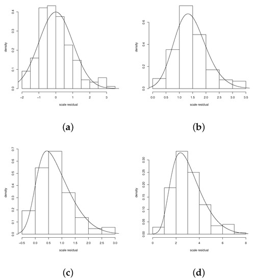
Figure 2. Histogram for scaled residuals for (a) Normal model, (b) PN model, (c) SN model, and (d) LGN model fitted to the cholesterol data.

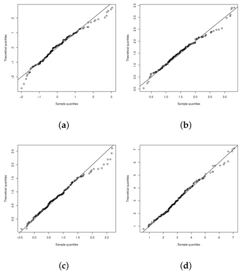
Figure 3. QQplots for (a) Normal model, (b) PN model, (c) SN model, and (d) LGN model fitted to the cholesterol data.

The normality assumption for errors can be tested by the hypothesis

$$H_{01}:(\delta ,\gamma )=(1,1)\mathrm{versus}{H}_{11}:(\delta ,\gamma )\ne (1,1),$$

using the likelihood-ratio (LR) statistics, $-2log\left({\mathrm{\Lambda }}_1\right)=-2\left({\ell }_N\left(\widehat{\mathbf{\theta }}\right)-{\ell }_{LGN}\left(\widehat{\mathbf{\theta }}\right)\right)$, which for the dataset under study, leads to $-2log\left({\mathrm{\Lambda }}_1\right)=18.228,$ so that p-value $<0.05$, with strong indication against the null hypothesis.

Similarly, the assumption of PN distribution for the errors can be tested by the hypothesis

$$H_{02}:\delta =1\mathrm{versus}{H}_{12}:\delta \ne 1,$$

using the LR statistics, $-2log\left({\mathrm{\Lambda }}_2\right)=-2\left({\ell }_{PN}\left(\widehat{\mathbf{\theta }}\right)-{\ell }_{LGN}\left(\widehat{\mathbf{\theta }}\right)\right)$, which leads to $-2log\left({\mathrm{\Lambda }}_2\right)=6.622,$ so that p-value $<0.05$, with strong indication against the null hypothesis.

Table 5 presents the AIC, AICc and BIC criteria for the normal, PN, SN and LGN models. Please note that according to these criteria, the model that best fits the dataset is the SN, since it has a lower value of AIC, AICc and BIC, followed by the LGN model. However, we remember that the SN model presents a singular information matrix when the asymmetry parameter $\lambda$ is zero, and therefore, hypothesis tests about the model parameters using likelihood-ratio statistics are not feasible from the theory of large samples; for example, for testing the significance of the asymmetry parameter in the SN model. This constitutes a disadvantage related to the LGN model, for which it was shown that it has a non-singular information matrix. In addition, as mentioned in Section 2, the LGN model has higher ranges of asymmetry and kurtosis than the SN model, so in practice it may be preferable in certain situations.

Table 5. AIC, AICc, and BIC for normal, PN and LGN linear models.

Criteria	Normal Model	PN Model	SN Model	LGN Model
AIC	1789.584	1779.979	1773.770	1775.356
AICc	1789.817	1780.331	1764.123	1775.853
BIC	1799.096	1795.832	1789.622	1794.379

This discussion illustrates that the final selection of a model is often simply a matter of choice. The LGN model can be considered appropriate if we want to use a model with which we can carry out hypothesis tests about the parameters, especially those associated with skewness and kurtosis in the model. In any case, the final choice must be duly justified.

For non-nested models, we used a generalized LR statistic test studied by Vuong [28]. This test was derived to compare competing models that are strictly non-nested. Since $F_{\theta }$ and $G_{\zeta }$ are two non-nested models, $f(y_i\mid x_i,\theta )$ and $g(y_i\mid x_i,\zeta )$ two densities corresponding to these non-nested models, the LR statistics to compare both models is given by

$$LR\left(\widehat{\theta },\widehat{\zeta }\right)=\left\{\frac{1}{\sqrt{n}}\sum _{i=1}^{n}log\frac{f\left(y_i\mid x_i,\widehat{\theta }\right)}{g\left(y_i\mid x_i,\widehat{\zeta }\right)}\right\},$$

which does not follow a chi-square distribution. To overcome this problem, Vuong [28] proposed an alternative approach based on the Kullback–Liebler information criterion [29]. Based on the distance between each model and the true process generating the data, namely the model $h^0(y\mid x)$, he arrived at the statistics

$$T_{LR,NN}=\frac{1}{\sqrt{n}}\frac{LR\left(\widehat{\theta },\widehat{\zeta }\right)}{\widehat{w}},$$

(13)

where

$${\widehat{w}}^2=\frac{1}{n}\sum _{i=1}^n{\left(log\frac{f\left(y_i\mid x_i,\widehat{\theta }\right)}{g\left(y_i\mid x_i,\widehat{\zeta }\right)}\right)}^2-{\left(\frac{1}{n}\sum _{i=1}^{n}log\frac{f\left(y_i\mid x_i,\widehat{\theta }\right)}{g\left(y_i\mid x_i,\widehat{\zeta }\right)}\right)}^2.$$

For strictly non-nested models, the statistic (13) converges in distribution to a standard normal distribution under the null hypothesis of equivalence of the models. Thus, the null hypothesis is not rejected if $|T_{LR,NN}|\le z_{p/2}$. On the other hand, we reject at significance level p the null hypothesis of equivalence of the models in favor of model $F_{\theta }$ being better (or worse) than model $G_{\zeta }$ if $T_{LR,NN}>z_p$ (or $T_{LR,NN}<-z_p$).

We now use Voung for comparing the LGN versus SN and PN versus SN models fitted to the data, since they are two non-nested models. Let $f\left(y_i\mid x_i,\widehat{\theta }\right)$ be the LGN model and $g\left(y_i\mid x_i,\widehat{\zeta }\right)$ the SN model. The generalized LR test statistic value is $T_{LR,NN}=33.981$. For PN versus SN, the generalized LR test statistic value is $T_{LR,NN}=30.072.$ Therefore, the LGN and PN models are significantly superior to the $SN$ model, according to the generalized LR statistic. Then, the LGN model is the better model compared with the normal, PN and SN models.

6.2. Application 2

For the second application, we consider a dataset consisting of measurements for 68 solar-type stars. These data were previously described and analyzed by Santos et al. [30] and Tovar-Falón et al. [31]. The dataset is available in the astrodatR library of the R Development Core Team [23] package under the name Stellar Abundances. In this application, we consider the response variable: $logN\left(Be\right)$, which represents the log of the abundance of beryllium scaled to Sun’s abundance, i.e., the Sun has $logN\left(Be\right)=0.0$. The explanatory variable is $\mathrm{Teff}/1000$, which represents the effective stellar surface temperature (in Kelvin).

In astronomy, objects such as stars, galaxies or X-ray sources, among others, are observed in some new wave bands. Some of these objects can go unnoticed due to limited sensitivities, leading to upper limits in the measurement of their luminosity (see Feilgelson [32]). For the dataset, 14 observations (19.35%) were censored at 0.0, i.e., 12 beryllium measurements were not detected.

We fitted the censored normal (CN) or Tobit model using the censReg function of R Development Core Team [23]. Likewise, we also fitted the censored power-normal (CPN) and censored LGN (CLGN) models. The Table 6 shows the MLEs of the fitted models. The initial values for the parameters ${\beta }_k$ were initially taken from those returned by the censReg package of the CN model. The outputs show that the explanatory variable X is significant in the considered models.

Table 6. Estimates (standard error) for CN, CPN, and CLGN linear models.

Parameters	CN Model	CPN Model	CLGN Model
${\beta }_0$	−0.9450 (0.5854)	−1.6054 (0.6910)	−1.1897 (0.4331)
${\beta }_1$	0.3224 (0.1023)	0.5222 (0.1208)	0.3520 (0.0732)
$\sigma$	0.3147 (0.0281)	0.0813 (0.0688)	0.3268 (0.0326)
$\alpha$	-	-	2.0123 (0.5762)
$\lambda$	-	0.0280 (0.0477)	4.5803 (0.9748)

Table 7 contains the AIC and AICC values for the fitted models, where it is observed that the CLGN model presents the best fit. Figure 4a–c show the histogram, the CDF and the qqplot of the CLGN model of the scale residual errors of the uncensored part. Here one can see the good fit of the CLGN model.

Table 7. AI and AICC for CN, CPN and CLGN linear models.

Criteria	CN Model	CPN Model	CLGN Model
AIC	50.2585	63.9628	−25.8152
AICC	50.6335	64.5977	−24.8474
BIC	62.9170	72.8408	−14.7176

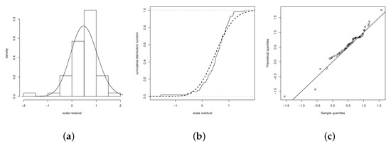
Figure 4. (a) histogram for scaled residuals CLGN model, (b) CDF of the scaled residuals CLGN model (c) qqplot for scaled residuals CLGN regression model.

We compare the Normal and PN models against the LGN model, so for hypothesis testing

$$(\delta ,\gamma )=(1,1)\mathrm{versus}(\delta ,\gamma )\ne (1,1)$$

and

$$\delta =1\mathrm{versus}\delta \ne 1,$$

we have $-2log\left({\Delta }_1\right)=8.4432$ and $-2log\left({\Delta }_2\right)=20.1476$ both statistics with p-$\mathrm{value}<0.05$ for which both tests are rejected and therefore the LGN model performs better than the Normal and PN models.

7. Conclusions

In this paper, we have proposed the asymmetric LGN distribution to give flexibility to the term of error in linear regression models. The LGN is based on the log-gamma-generated families of distributions of Amini et al. [15]. This new model presents greater ranges of asymmetry and kurtosis, and it extends the PN family of distribution; therefore, it has more flexibility in terms of asymmetry and kurtosis. The ordinary Tobit model Tobin [24] and the Tobit power-normal model Martínez-Flórez et al. [25] are special cases from an extension of the studied model LGN to the case of censored data. The maximum likelihood method was implemented, and the Fisher information matrix was derived, and it was shown numerically to be non-singular, which guarantees valid large sample results for the likelihood-ratio statistics. Two illustrations of real data reveal that the proposed model can be a useful alternative to existing models such as normal, power-normal, Tobit normal and Tobit power-normal. In addition, under certain considerations such as the non-singularity of the information matrix of the model and larger ranges of asymmetry and kurtosis, it may be a better alternative to the skew-normal distribution.

References

- Azzalini, A. A class of distributions which includes the normal ones. Scand. J. Stat. 1985, 12, 171–178. [Google Scholar]
- Durrans, S.R. Distributions of fractional order statistics in hydrology. Water Resour. Res. 1992, 28, 1649–1655. [Google Scholar] [CrossRef]
- Gupta, R.D.; Gupta, R.C. Analyzing skewed data by power normal model. Test 2008, 17, 197–210. [Google Scholar] [CrossRef]
- Pewsey, A.; Gómez, H.W.; Bolfarine, H. Likelihood-based inference for power distributions. Test 2012, 21, 775–789. [Google Scholar] [CrossRef]
- Martínez-Flórez, G.; Bolfarine, H.; Gómez, H.W. Skew-normal alpha-power model. Statistics 2014, 48, 1414–1428. [Google Scholar] [CrossRef]
- Martínez-Flórez, G.; Vergara-Cardozo, S.; González, L.M. The family of log-skew-normal alpha-power distributions using precipitation data. Rev. Colomb. Estad. 2013, 36, 43–57. [Google Scholar]
- Tovar-Falón, R.; Bolfarine, H.; Martínez-Flórez, G. The Asymmetric Alpha-Power Skew-t Distribution. Symmetry 2020, 12, 82. [Google Scholar] [CrossRef] [Green Version]
- Azzalini, A.; Capitanio, A. Distributions generated by perturbation of symmetry with emphasis on a multivariate skew-t distribution. J. R. Stat. Soc. Ser. B (Stat. Methodol.) 2003, 65, 367–389. [Google Scholar] [CrossRef]
- Zhao, J.; Kim, H.M. Power-t distributions. Commun. Stat. Appl. Methods 2016, 23, 321–334. [Google Scholar]
- Tung, H.P.; Tseng, S.T.; Hsu, N.J.; Hou, Y.T. A generalized pH acceleration model of nano-sol products and the effects of model misspecification on shelf-life prediction. IISE Trans. 2022, 54, 496–504. [Google Scholar] [CrossRef]
- Martínez-Flórez, G.; Tovar-Falón, R.; Jimémez-Narváez, M. Likelihood-Based Inference for the Asymmetric Beta-Skew Alpha-Power Distribution. Symmetry 2020, 12, 613. [Google Scholar] [CrossRef]
- Martínez-Flórez, G.; Tovar-Falón, R.; Martínez-Guerra, M. The Censored Beta-Skew Alpha-Power Distribution. Symmetry 2021, 13, 1114. [Google Scholar] [CrossRef]
- Sahu, S.K.; Dey, D.K.; Branco, M.D. A new class of multivariate skew distributions with applications to Bayesian regression models. Can. J. Stat. 2003, 31, 129–150. [Google Scholar] [CrossRef] [Green Version]
- Martínez-Flórez, G.; Bolfarine, H.; Gómez, H.W. Asymmetric regression models with limited responses with an application to antibody response to vaccine. Biom. J. 2013, 55, 156–172. [Google Scholar] [CrossRef]
- Amini, M.; MirMostafaee, S.M.T.K.; Ahmani, J. Log–gamma–generated families of distributions. Statistics 2014, 48, 913–926. [Google Scholar] [CrossRef]
- Cordeiro, G.M.; Bourguignon, M.; Ortega, E.M.M.; Ramires, T.G. General mathematical properties, regression and applications of the log-gamma-generated family. Commun. Stat.—Theory Methods 2018, 47, 1050–1070. [Google Scholar] [CrossRef]
- Prentice, R.L. A log-gamma model and its maximum likelihood estimation. Biometrika 1974, 61, 539–544. [Google Scholar] [CrossRef]
- Lawless, J.F. Inference in the generalized gamma and log gamma distributions. Technometrics 1980, 22, 409–419. [Google Scholar] [CrossRef]
- Young, D.H.; Bakir, S.T. Bias correction for a generalized log-gamma regression model. Technometrics 1987, 29, 183–191. [Google Scholar] [CrossRef]
- Ortega, E.M.M.; Bolfarine, H.; Paula, G.A. Influence diagnostics in generalized log-gamma regression models. Comput. Stat. Data Anal. 2003, 42, 165–186. [Google Scholar] [CrossRef]
- Ortega, E.M.M.; Cancho, V.G.; Paula, G.A. Generalized log-gamma regression models with cure fraction. Lifetime Data Anal. 2009, 15, 79. [Google Scholar] [CrossRef] [PubMed]
- Zhang, D.; Davidian, M. Linear mixed models with flexible distributions of random effects for longitudinal data. Biometrics 2001, 57, 795–802. [Google Scholar] [CrossRef] [PubMed]
- R Development Core Team. R: A Language and Environment for Statistical Computing; R Foundation for Statistical Computing: Vienna, Austria, 2021; Available online: http://www.R-project.org (accessed on 31 July 2021).
- Tobin, J. Estimation of relationship for limited dependent variables. Econometrica 1958, 26, 24–36. [Google Scholar] [CrossRef] [Green Version]
- Martínez-Flórez, G.; Bolfarine, H.; Gómez, H.W. The alpha–power tobit model. Commun. Stat.—Theory Methods 2013, 42, 633–643. [Google Scholar] [CrossRef]
- Akaike, H. A new look at statistical model identification. IEEE Trans. Autom. Control 1974, 19, 716–722. [Google Scholar] [CrossRef]
- Schwarz, G. Estimating the dimension of a model. Ann. Stat. 1978, 6, 461–464. [Google Scholar] [CrossRef]
- Vuong, Q.H. Likelihood ratio tests for models selection and non–nested hypotheses. Econometrica 1989, 57, 307–333. [Google Scholar] [CrossRef] [Green Version]
- Kleiber, C.; Zeileis, A. Applied Econometrics with R, 1st ed.; Springer: New York, NY, USA, 2008. [Google Scholar]
- Santos, N.; López, R.G.; Israelian, G.; Mayor, M.; Rebolo, R.; García-Gil, A.; De Taoro, M.P.; Randich, S. Beryllium abundances in stars hosting giant planets. Astron. Astrophys. 2002, 386, 1028–1038. [Google Scholar] [CrossRef]
- Tovar-Falón, R.; Bolfarine, H.; Martínez-Flórez, G. The Asymmetric Power-Student-t Model for Censored and Truncated Data. Acad. Bras. Cienc. 2021, 93, e20190920. [Google Scholar] [CrossRef]
- Feilgelson, E.D. astrodatR: Astronomical Data. R Package v. 0.1. Available online: https://cran.r-project.org/web/packages/astrodatR/ (accessed on 31 July 2021).
Publisher’s Note: MDPI stays neutral with regard to jurisdictional claims in published maps and institutional affiliations. |
© 2022 by the authors. Licensee MDPI, Basel, Switzerland. This article is an open access article distributed under the terms and conditions of the Creative Commons Attribution (CC BY) license (https://creativecommons.org/licenses/by/4.0/).