A Boundary Element Procedure for 3D Electromagnetic Transmission Problems with Large Conductivity

Abstract

We consider the scattering of time-periodic electromagnetic fields by metallic obstacles, or the eddy current problem. In this interface problem, different sets of Maxwell equations must be solved both in the obstacle and outside it, while the tangential components of both electric and magnetic fields are continuous across the interface. We describe an asymptotic procedure, applied for large conductivity, which reflects the skin effect in metals. The key to our method is a special integral equation procedure for the exterior boundary value problems corresponding to perfect conductors. The asymptotic procedure leads to a great reduction in complexity for the numerical solution, since it involves solving only the exterior boundary value problems. Furthermore, we introduce a FEM/BEM coupling procedure for the transmission problem and consider the implementation of Galerkin’s elements for the perfect conductor problem, and present numerical experiments.

1. Introduction

We present asymptotic expansions with respect to inverse powers of conductivity for the electrical and magnetic fields and report the algorithm of MacCamy and Stephan [1], which allows us to compute the expansion terms of the electrical field in the exterior domain by successively solving only exterior problems (so-called perfect conductor problems). We use various data for the interfaces between the conductors (metal) and the isolator (air). We solve the exterior problems numerically by applying the Galerkin boundary element method to boundary integral equations of the first kind, which were originally introduced by MacCamy and Stephan in [2]. This system of integral equations on the interface $\Sigma$ results from a single layer ansatz for the electrical field and has unknown densities, namely, a vector field and a scalar function on $\Sigma$ which we approximate with lower-order Raviart Thomas elements and continuous piecewise linear functions on a regular, triangular mesh on $\Sigma$. As in the two dimensional case investigated by Hariharan [3,4] and MacCamy and Stephan [5], the asymptotic procedure gives for the computation of the solution of the transmission problem a great reduction in complexity, since it involves solving only the exterior problem, and furthermore, only a few expansion terms must be computed. We describe in detail how to implement the boundary element method for the perfect conductor problem. As an alternative to the asymptotic expansions for the solution of the transmission problem, we introduce a new finite element/boundary element Galerkin coupling procedure which converges quasi-optimally toward the energy norm.

2. Asymptotic Expansion for Large Conductivity and Skin Effect

Let ${\Omega }_{-}$ be a bounded region in ${\mathbb{R}}^3$ representing a metallic conductor and ${\Omega }_{+}:={\mathbb{R}}^3\backslash \overline{{\Omega }_{-}}$ represent air. The parameters ${\epsilon }_0$, ${\mu }_0$, ${\sigma }_0$ denoting permittivity, permeability and conductivity, are assumed to be zero in ${\Omega }_{+}$ with positive $\epsilon$, $\mu$ and $\sigma$ values in ${\Omega }_{-}$. Let the incident electric and magnetic fields, ${\mathbf{E}}^0$ and ${\mathbf{H}}^0$, satisfy Maxwell’s equations in air. The total fields $\mathbf{E}$ and $\mathbf{H}$ satisfy the same Maxwell’s equations as ${\mathbf{E}}^0$ and ${\mathbf{H}}^0$ in ${\Omega }_{+}$, but a different set of equations in ${\Omega }_{-}$. Across the interface $\Sigma :=\partial {\Omega }_{-}=\partial {\Omega }_{+}$, which is assumed to be a regular analytic surface, the tangential components of both $\mathbf{E}$ and $\mathbf{H}$ are continuous. $\mathbf{E}-{\mathbf{E}}^0$ and $\mathbf{H}-{\mathbf{H}}^0$ represent the scattered fields. All fields are time-harmonic with frequency $\omega$. As in [1], we neglect conduction (displacement) currents in air (metal).

Then, with appropriate scaling, the eddy current problem is (see [6,7]).

Problem $\left({\mathit{P}}_{\alpha \beta }\right)$: Given $\alpha >0$ and $\beta >0$, find $\mathbf{E}$ and $\mathbf{H}$, such that

$$\begin{array}{ccc}\mathrm{curl}\mathbf{E}=\mathbf{H},\hfill & \mathrm{curl}\mathbf{H}={\alpha }^2\mathbf{E}\hfill & in{\Omega }_{+}\left(\mathrm{air}\right)\hfill \\ \mathrm{curl}\mathbf{E}=\mathbf{H},\hfill & \mathrm{curl}\mathbf{H}=i{\beta }^2\mathbf{E}\hfill & in{\Omega }_{-}\left(\mathrm{metal}\right)\hfill \\ {\mathbf{E}}_T^{+}={\mathbf{E}}_T^{-},\hfill & {\mathbf{H}}_T^{+}={\mathbf{H}}_T^{-},\hfill & \mathrm{on}\Sigma .\hfill \end{array}$$

(1)

$${\displaystyle \frac{\partial }{\partial r}}\mathbf{E}\left(\mathit{x}\right)-i\alpha \mathbf{E}\left(\mathbf{x}\right)=O\left({\displaystyle \frac{1}{r^2}}\right)withr=\left|\mathbf{x}\right|,\mathrm{as}\left|\mathbf{x}\right|\to \infty .$$

Here ${\alpha }^2={\omega }^2{\mu }_0{\epsilon }_0$ and ${\beta }^2=\omega \mu \sigma -i{\omega }^2\mu \epsilon$ are dimensionless parameters, and ${\beta }^2=\omega \mu \sigma >0$, if displacement currents are neglected in metal $(\epsilon =0)$. The subscript T denotes a tangential component, and the superscripts plus and minus denote limits from ${\Omega }_{+}$ and ${\Omega }_{-}$.

At higher frequencies, the constant $\beta$ is usually large, leading to the perfect conductor approximation. Formally this means solving only the ${\Omega }_{+}$ equation and requiring that ${\mathbf{E}}_T=0$ on $\Sigma$. If we let $\mathbf{E}$ and $\mathbf{H}$ denote the scattered fields, we obtain

Problem $\left({\mathit{P}}_{\alpha \infty }\right)$: Given $\alpha >0$, find $\mathbf{E}$ and $\mathbf{H}$, such that

$$\begin{array}{ccc}\hfill \mathrm{curl}\mathbf{E}=\mathbf{H},& \hfill \mathrm{curl}\mathbf{H}={\alpha }^2\mathbf{E}& \hfill \mathrm{in}{\Omega }_{+}\\ \hfill & \hfill {\mathbf{E}}_T=-{\mathbf{E}}_T^0,& \hfill \mathrm{on}\Sigma .\end{array}$$

(2)

Remark 1.

There exists at most one solution of problem $\left({\mathit{P}}_{\alpha \beta }\right)$ for any $\alpha >0$ and $0<\beta \le \infty$ (see [8]).

Remark 2.

There exists a sequence ${\left\{{\alpha }_k\right\}}_{k=1}^{\infty }$, such that if $\alpha \ne {\alpha }_k$, then curl$\mathit{E}=\mathit{H}$, $curl\mathit{H}={\alpha }^2\mathit{E}$ in ${\Omega }_{+}$, ${\mathit{E}}_T\equiv 0$ on Σ implies $\mathit{E}\equiv \mathit{H}\equiv 0$ in ${\Omega }_{+}$.

We are interesting in an asymptotic expansion of the solution of problem $\left({\mathbf{P}}_{\alpha \beta }\right)$ with respect to inverse powers of conductivity. With $\tau$ denoting the distance from $\Sigma$ measured into ${\Omega }_{-}$ along the normal to $\Sigma$, the expansions reads:

$$\mathbf{E}\sim {\mathbf{E}}^0+\sum _{n=0}^{\infty }{\mathbf{E}}_n{\beta }^{-n}\mathrm{in}{\Omega }_{+}$$

(3)

$$\mathbf{H}\sim {\mathbf{H}}^0+\sum _{n=0}^{\infty }{\mathbf{H}}_n{\beta }^{-n}\mathrm{in}{\Omega }_{+}$$

(4)

$$\mathbf{E}\sim e^{-\sqrt{-i}\beta \tau }\sum _{n=0}^{\infty }{\mathbf{E}}_n{\beta }^{-n}\mathrm{in}{\Omega }_{-}$$

(5)

$$\mathbf{H}\sim e^{-\sqrt{-i}\beta \tau }\sum _{n=0}^{\infty }{\mathbf{H}}_n{\beta }^{-n}\mathrm{in}{\Omega }_{-}$$

(6)

Here ${\mathbf{E}}_n$ and ${\mathbf{H}}_n$ are independent of $\beta$, which is proportional to $\sqrt{\sigma }$. The exponential in (5) and (6) represents the skin effect. Next, we present from [1] these expansions for the half-space case where the various coefficients can be computed recursively. Note ${\mathbf{E}}_0$ and ${\mathbf{H}}_0$ in (3) and (4), respectively, are simply the perfect conductor approximation, that is, the solution of $\left({\mathbf{P}}_{\alpha \infty }\right)$. ${\mathbf{E}}_n$ and ${\mathbf{H}}_n$ in (3) and (4) can be calculated successively by solving a sequence of problems of the same form as $\left({\mathbf{P}}_{\alpha \infty }\right)$ but with boundary values determined from earlier coefficients. The ${\mathbf{E}}_n$ and ${\mathbf{H}}_n$ in (5) and (6), respectively, are obtained by solving ordinary differential equations in the variable $x_3$.

For the ease of the reader, we present here in the half-space case ${\Omega }_{+}={\mathbb{R}}_{+}^3$, i.e., $x_3>0$, and ${\Omega }_{-}={\mathbb{R}}_{-}^3$, i.e., $x_3<0$, a formal procedure to compute ${\mathbf{E}}_n$, ${\mathbf{H}}_n$, which was given by MacCamy and Stephan [1]. They substituted Equations (3)–(6) into $\left({\mathbf{P}}_{\alpha \beta }\right)$ for $\Sigma ={\mathbb{R}}^2$ and equated coefficients of ${\beta }^{-n}$. Here, we give a short description of their approach.

Let $\chi =e^{\sqrt{-i}\beta x_3}$ and decompose field $\mathbf{F}$ into tangential and normal components:

$$\mathbf{F}=\mathfrak{F}+f{\mathbf{e}}_3,\mathfrak{F}={\mathcal{F}}^1{\mathbf{e}}_1+{\mathcal{F}}^2{\mathbf{e}}_2,$$

(7)

with orthogonal component ${\mathfrak{F}}^{\perp }={\mathbf{e}}_3\times \mathfrak{F}$, and unit vectors ${\mathbf{e}}_i$ ($i=1,2,3$).

Then, one computes with the surface gradient ${\mathrm{grad}}_T$, the rotation

$$\mathrm{curl}\mathbf{F}={\mathfrak{F}}_{x_3}^{\perp }-{\left({\mathrm{grad}}_{T}f\right)}^{\perp }-\left(\mathrm{div}{\mathfrak{F}}^{\perp }\right){\mathbf{e}}_3$$

(8)

and

$$\mathrm{curl}\left(\chi \mathbf{F}\right)=\chi [\sqrt{-i}\beta {\mathfrak{F}}^{\perp }+{\mathfrak{F}}_{x_3}^{\perp }-{\left({\mathrm{grad}}_{T}f\right)}^{\perp }-\left(\mathrm{div}{\mathfrak{F}}^{\perp }\right){\mathbf{e}}_3].$$

(9)

Now, by setting ${\mathbf{E}}_n={\mathcal{E}}_n+{\ell }_n{\mathbf{e}}_3$, one obtains for $x_3<0$

$$\mathrm{curl}\mathbf{E}\sim \chi \{\sqrt{-i}\beta {\mathcal{E}}_0^{\perp }+\sum _{n=0}^{\infty }[\sqrt{-i}{\mathcal{E}}_{n+1}^{\perp }+{\mathcal{E}}_{n,x_3}^{\perp }-{\left({\mathrm{grad}}_T{\ell }_n\right)}^{\perp }-\left(\mathrm{div}{\mathcal{E}}_n^{\perp }\right){\mathbf{e}}_3]{\beta }^{-n}\},$$

(10)

and

$$\begin{array}{cc}\hfill \mathrm{curl}\mathrm{curl}\mathbf{E}& \sim \chi \left\{i{\beta }^2{\mathcal{E}}_0-\sqrt{-i}\beta {\mathcal{E}}_{0,x_3}+\sqrt{-i}\beta \mathrm{div}{\mathcal{E}}_0{\mathbf{e}}_3+\sum _{n=0}^{\infty }\left[i\beta {\mathcal{E}}_{n+1}-\sqrt{-i}{\mathcal{E}}_{n+1,x_3}\right.\right.\hfill \\ \hfill & -\sqrt{-i}\mathrm{div}{\mathcal{E}}_{n+1}{\mathbf{e}}_3-\sqrt{-i}\beta {\mathcal{E}}_{n,x_3}-{\mathcal{E}}_{n,x_3,x_3}+\mathrm{div}{\mathcal{E}}_{n,x_3}{\mathbf{e}}_3+\sqrt{-i}\beta \mathrm{grad}{\ell }_n\hfill \\ \hfill & \left.\left.+{\left({\mathrm{grad}}_T{\ell }_n\right)}_{x_3}+\mathrm{div}\mathrm{grad}{\ell }_n{\mathbf{e}}_3\right]{\beta }^{-n}+\mathrm{grad}\mathrm{div}{\beta }^{-n}{\mathbf{e}}_3\right\}\hfill \\ \hfill & =\chi [i{\beta }^2{\mathcal{E}}_0+i{\beta }^2{\ell }_0{\mathbf{e}}_3+i\beta {\mathcal{E}}_1+i\beta {\ell }_1{\mathbf{e}}_3+\sum _{n=0}^{\infty }(i{\mathcal{E}}_{n+2}+i{\ell }_{n+2}{\mathbf{e}}_3){\beta }^{-n}]\sim i{\beta }^2\mathbf{E}.\hfill \end{array}$$

(11)

Hence, matching coefficients of ${\beta }^2$ and $\beta$, respectively, yields ${\ell }_0\equiv 0$, $i{\ell }_1=\sqrt{-i}\mathrm{div}{\mathcal{E}}_0$ and ${\mathcal{E}}_{0,x_3}=0$ implying ${\mathcal{E}}_0(x_1,x_2,x_3)={\mathcal{E}}_0(x_1,x_2,0)$.

As coefficients of ${\beta }^0$, one obtains

$$-\sqrt{-i}{\mathcal{E}}_{1,x_3}+\sqrt{-i}\mathrm{grad}{\ell }_1=0,$$

$$\sqrt{-i}\mathrm{div}{\mathcal{E}}_1+\mathrm{div}{\mathcal{E}}_{0,x_3}-\mathrm{grad}\mathrm{div}{\mathcal{E}}_0=i{\ell }_2.$$

Now the gauge condition $\mathrm{div}{\mathcal{E}}_0=0$ implies ${\ell }_1\equiv 0$ and $\mathrm{div}{\mathcal{E}}_{0,x_3}=0$; hence ${\mathcal{E}}_{1,x_3}=0$ and $\sqrt{-i}\mathrm{div}{\mathcal{E}}_1=i{\ell }_2.$ Thus, ${\mathcal{E}}_1(x_1,x_2,x_3)={\mathcal{E}}_1(x_1,x_2,0)$.

Equating coefficients of ${\beta }^{-1}$ in (11) gives

$$-\sqrt{-i}{\mathcal{E}}_{2,x_3}-\sqrt{-i}{\mathcal{E}}_{2,x_3}+\sqrt{-i}\mathrm{grad}{\ell }_2=0,$$

$$\sqrt{-i}\mathrm{div}{\mathcal{E}}_2-\mathrm{grad}\mathrm{div}{\mathcal{E}}_1=i{\ell }_3.$$

Setting

$$\mathbf{H}=\chi \sum _{n=0}^{\infty }({\mathcal{H}}_n+h_n{\mathbf{e}}_3){\beta }^{-n},$$

(12)

MacCamy and Stephan obtained in [1] with ${\ell }_1=0$, $h_0=0$, ${\mathcal{E}}_0=0$:

$$\sqrt{-i}{\mathcal{E}}_1^{\perp }+{\mathcal{E}}_{0,x_3}^{\perp }={\mathcal{H}}_0,\sqrt{-i}{\mathcal{H}}_0^{\perp }=i{\mathcal{E}}_1,h_0=\mathrm{div}{\mathcal{E}}_0^{\perp }=0.$$

(13)

and

$$\sqrt{-i}{\mathcal{E}}_2^{\perp }+{\mathcal{E}}_{1,x_3}^{\perp }={\mathcal{H}}_1,\sqrt{-i}{\mathcal{H}}_1^{\perp }+{\mathcal{H}}_{0,x_3}^{\perp }=i{\mathcal{E}}_2$$

(14)

$$h_1=-\mathrm{div}{\mathcal{E}}_1^{\perp },-\mathrm{div}{\mathcal{H}}_0^{\perp }=i{\ell }_2.$$

(15)

and

$$\begin{array}{c}{\mathcal{H}}_{0,x_3}\equiv {\mathcal{E}}_{1,x_3}\equiv 0\hfill \\ \\ {\mathcal{H}}_0\equiv \sqrt{-i}{\mathcal{E}}_1^{\perp }\hfill & \mathrm{in}& x_3<0\hfill \end{array}$$

(16)

For $x_3>0$, we have that $\mathrm{curl}\mathbf{E}=\mathbf{H}$ yields

$$\mathrm{curl}{\mathbf{E}}^0+\sum _{n=0}^{\infty }\mathrm{curl}{\mathbf{E}}_n{\beta }^{-n}={\mathbf{H}}^0+\sum _{n=0}^{\infty }{\mathbf{H}}_n{\beta }^{-n}.$$

Matching coefficients of ${\beta }^{-n}$, one finds in $x_3>0$

$$\mathrm{curl}{\mathbf{E}}^0={\mathbf{H}}^0,\mathrm{curl}{\mathbf{E}}_n={\mathbf{H}}_n,n\ge 0,$$

(and corresponding due to $\mathrm{curl}\mathbf{H}={\alpha }^2\mathbf{E}$)

$$\mathrm{curl}{\mathbf{H}}^0={\alpha }^2{\mathbf{E}}^0,\mathrm{curl}{\mathbf{H}}_n={\alpha }^2{\mathbf{E}}_n,n\ge 0.$$

With the above relations, the recursion process goes as follows. First one use (6.10) for $n=0$ and (6.13), in [1], to conclude that

$$\begin{array}{cccc}\mathrm{curl}{\mathbf{E}}_0={\mathbf{H}}_0,& \mathrm{curl}{\mathbf{H}}_0={\alpha }^2{\mathbf{E}}_0& \mathrm{in}& x_3>0\\ {\mathbf{E}}_0^{+}=-{\left({\mathbf{E}}_T^0\right)}^{-},& \mathrm{on}& x_3=0.\end{array}$$

Now $({\mathbf{E}}_0,{\mathbf{H}}_0)$ is just the solution of $\left({\mathbf{P}}_{\alpha \infty }\right)$, which can be solved by the boundary integral equation procedure introduced in MacCamy and Stephan [1] and revisited below. However, from ${\left(1\right)}_3$ we obtain

$${\mathcal{H}}_0^{-}={\mathcal{H}}_0^{+}={\left({\mathbf{H}}_0\right)}_T^{+}on{x}_3=0.$$

(17)

Now, the right side of (17) is known and easily computed. Then ${\left(1\right)}_3$ and (17) yield

$${\left({\mathbf{E}}_1\right)}_T^{+}={\left({\mathbf{E}}_1\right)}_T^{-}={\mathcal{E}}_1^{-}=-\sqrt{i}{\left({\mathcal{H}}_0^{\perp }\right)}^{-}=-\sqrt{i}{\left({\left({\mathbf{H}}_0\right)}_T^{+}\right)}^{\perp }.$$

(18)

Therefore, by (6.10), in [1], we have, again, a new solvable problem for $({\mathbf{E}}_1,{\mathbf{H}}_1)$ which is just like $\left({\mathbf{P}}_{\alpha \infty }\right)$, that is

$$\mathrm{curl}{\mathbf{E}}_1={\mathbf{H}}_1,\mathrm{curl}{\mathbf{H}}_1={\alpha }^2{\mathbf{E}}_1\mathrm{in}{x}_3>0,$$

but with new boundary values for ${\mathbf{E}}_T$ as given by (18).

For the complete algorithm see [1]. Note, with $\lambda =\sqrt{-i}$, we have ${\mathcal{E}}_1^{-}(x_1,x_2,0)=-{\displaystyle \frac{1}{\lambda }}(\mathbf{n}\times \mathrm{curl}{\mathbf{E}}_0)$ yielding in $x_3<0$

$${\mathbf{E}}_1(x_1,x_2,x_3)={\int }_0^{-\tau }{e}^{\lambda \beta {\tilde{x}}_3}{\mathcal{E}}_1^{-}(x_1,x_2,0)d{\tilde{x}}_3=-{\displaystyle \frac{1}{{\lambda }^2\beta }}(\mathbf{n}\times \mathrm{curl}{\mathbf{E}}_0)[e^{-\lambda \beta \tau }-1]$$

A comparison with Peron’s results (see Chapter 5 in [9]) shows that ${\mathbf{W}}_j^{cd}(y_{\alpha },h_{\rho })=e^{-\sqrt{-i}\beta \tau }{\mathbf{E}}_j$, $j\ge 0$, in ${\Omega }^{cd}$, $\lambda Y_3=\sqrt{-i}\beta \tau$ and $w_j={\ell }_j$. Furthermore, we see that the first terms in the asymptotic expansion of the electrical field for a smooth surface $\Sigma$ derived by Peron coincide with those for the half-space $x_3=0$ investigated by MacCamy and Stephan, namely, ${\ell }_0=w_0=0$, ${\ell }_1=w_1=0$, ${\mathcal{E}}_0={\mathbf{W}}_0^{cd}=0$.

Remark 3.

From Theorem 5 in Chapter 3 of [10], there exists only one solution to the electromagnetic transmission problem for a smooth interface. This solution which can be computed by the boundary integral equation procedure is shown below, where we assume that (19) holds. Then, for the electrical field $\mathit{E}$ obtained via the boundary integral equation system, we have that in the tubular region ${\Omega }_{\pm }\left(\delta \right)=\left\{x\in {\Omega }_{\pm },dist(x,\Sigma )<\delta \right\}$, there holds for the remainders ${\mathit{E}}_m^{is\left(cd\right)}$ obtained by truncating (3) and (5) at $n=m$

$${\parallel {\mathit{E}}_{m,\rho }^{is}\parallel }_{\mathit{W}(curl,{\Omega }^{is})}\le C_1{\rho }^{-m-1}and\parallel {\mathit{E}}_{m,\rho }^{cd}\parallel \le C_2{e}^{C_3\tau }$$

for constants $C_1,C_2,C_3>0$, independent of ρ.

3. A Boundary Integral Equation Method of the First Kind

Next, we describe the integral equation procedure for $\left({\mathbf{P}}_{\alpha \beta }\right)$ and $\left({\mathbf{P}}_{\alpha \infty }\right)$ from [1,7,11,12]. Throughout the section, we require that

$$\alpha \ne {\alpha }_k,k=1,2,\dots$$

(19)

These methods, like others, are based on the Stratton–Chu formulas from [6]. To describe these, some notation is needed. Let $\mathbf{n}$ denote the exterior normal to $\Sigma$. Given any vector field $\mathbf{v}$ defined on $\Sigma$, we have

$$\mathbf{v}={\mathbf{v}}_T+v_N\mathbf{n},{\mathbf{v}}_T=\mathbf{n}\times (\mathbf{v}\times \mathbf{n})$$

(20)

where ${\mathbf{v}}_T$, which lies in the tangent plane, is the tangential component of $\mathbf{v}$.

Define the simple layer potential ${\mathcal{V}}_{\kappa }$ for density $\psi$ (correspondingly for a vector field) for the surface $\Sigma$ by

$${\mathcal{V}}_{\kappa }\left(\psi \right)={\int }_{\Sigma }\psi \left(\mathbf{y}\right)G_{\kappa }\left(\right|\mathbf{x}-\mathbf{y}\left|\right)d{s}_y,\mathrm{with}{G}_{\kappa }\left(r\right)={\displaystyle \frac{e^{i\kappa r}}{4\pi r}}.$$

(21)

For a vector field $\mathbf{v}$ on $\Sigma$, define ${\mathcal{V}}_{\kappa }\left(\mathbf{v}\right)$ by (21) with $\mathbf{v}$ replacing $\psi$.

We collect in the following lemma some of the well-known results about the simple layer potential ${\mathcal{V}}_{\kappa }$.

Remark 4

(Lemma 2.1 in [1]). For any complex κ, $0\le arg \kappa \le {\displaystyle \frac{\pi }{2}}$ and any continuous ψ on Σ, there holds:

(i) 

${\mathcal{V}}_{\kappa }\left(\psi \right)$ is continuous in ${\mathbb{R}}^3$,

(ii) 

$\Delta {\mathcal{V}}_{\kappa }\left(\psi \right)=-{\kappa }^2{\mathcal{V}}_{\kappa }\left(\psi \right)$ in ${\Omega }_{-}\cup {\Omega }_{+}$,

(iii) 

${\mathcal{V}}_{\kappa }\left(\psi \right)\left(\mathit{x}\right)=O\left({\displaystyle \frac{e^{i\kappa \left|\mathit{x}\right|}}{\left|\mathit{x}\right|}}\right)$ as $\left|\mathit{x}\right|\to \infty$,

(iv) 

$${\left({\displaystyle \frac{\partial {\mathcal{V}}_{\kappa }\left(\psi \right)}{\partial \mathbf{n}}}\left(\mathit{x}\right)\right)}^{\pm }=\mp {\displaystyle \frac{1}{2}}\psi \left(\mathit{x}\right)+{\int }_{\Sigma }{K}_{\kappa }(\mathit{x},\mathit{y})\psi \left(\mathit{y}\right)d{s}_y,on\Sigma ,$$

where $K_{\kappa }(\mathit{x},\mathit{y})={O\left(\right|\mathit{x}-\mathit{y}|}^{-1})$ as $\mathit{y}\to \mathit{x}$.

(v) 

$${(\mathit{n}\times curl{\mathcal{V}}_{\kappa }\left(\mathbf{v}\right)\left(\mathit{x}\right))}^{\pm }=\pm {\displaystyle \frac{1}{2}}\mathbf{v}\left(\mathit{x}\right)+{\displaystyle \frac{1}{2}}{\int }_{\Sigma }{\mathit{K}}_{\kappa }(\mathit{x},\mathit{y})\mathbf{v}\left(\mathit{y}\right)d{s}_y,$$

where the matrix function ${\mathit{K}}_{\kappa }$ satisfies ${\mathit{K}}_{\kappa }(\mathit{x},\mathit{y})=O\left({|\mathit{x}-\mathit{y}|}^{-1}\right)$ as $\mathit{y}\to \mathit{x}$.

For problem ${\left(1\right)}_2$ in ${\Omega }_{-}$, the Stratton–Chu formula gives

$$\begin{array}{c}\mathbf{E}={\mathcal{V}}_{\sqrt{i}\beta }(\mathbf{n}\times \mathbf{H})-\mathrm{curl}{\mathcal{V}}_{\sqrt{i}\beta }(\mathbf{n}\times \mathbf{E})+\mathrm{grad}{\mathcal{V}}_{\sqrt{i}\beta }(\mathbf{n}·\mathbf{E}),\hfill \\ \mathbf{H}=\mathrm{curl}{\mathcal{V}}_{\sqrt{i}\beta }(\mathbf{n}\times \mathbf{H})-\mathrm{curl}\mathrm{curl}{\mathcal{V}}_{\sqrt{i}\beta }(\mathbf{n}\times \mathbf{E}).\hfill \end{array}$$

(22)

Similarly, for problem ${\left(1\right)}_1$, in ${\Omega }_{+}$

$$\begin{array}{c}\mathbf{E}={\mathcal{V}}_{\alpha }(\mathbf{n}\times \mathbf{H})-\mathrm{curl}{\mathcal{V}}_{\alpha }(\mathbf{n}\times \mathbf{E})+\mathrm{grad}{\mathcal{V}}_{\alpha }(\mathbf{n}·\mathbf{E}),\hfill \\ \mathbf{H}=\mathrm{curl}{\mathcal{V}}_{\alpha }(\mathbf{n}\times \mathbf{H})-\mathrm{curl}\mathrm{curl}{\mathcal{V}}_{\alpha }(\mathbf{n}\times \mathbf{E}).\hfill \end{array}$$

(23)

For given $\mathbf{n}\times \mathbf{H}$, $\mathbf{n}\times \mathbf{E}$ and $\mathbf{n}·\mathbf{E}$, (23) yields a solution of $\left({\mathbf{P}}_{\alpha \infty }\right)$. However, we know only $\mathbf{n}\times \mathbf{E}$. The standard treatment of $\left({\mathbf{P}}_{\alpha \infty }\right)$ starts from (23), sets $\mathbf{n}\times \mathbf{H}=0$ and $\mathbf{n}·\mathbf{E}=0$ and replaces $-\mathbf{n}\times \mathbf{E}$ with an unknown tangential field $\mathbf{L}$ yielding

$$\mathbf{E}=\mathrm{curl}{\mathcal{V}}_{\alpha }\left(\mathbf{L}\right),\mathbf{H}=\mathrm{curl}\mathrm{curl}{\mathcal{V}}_{\alpha }\left(\mathbf{L}\right).$$

(24)

Then the boundary condition yields an integral equation of the second kind for $\mathbf{L}$ in the tangent space to $\Sigma$.

The method (24) is analogous to solving the Dirichlet problem for the scalar Helmholtz equation with a double layer potential. However, having found $\mathbf{L}$, it is hard to determine ${\mathbf{H}}_T$, or equivalently $\mathbf{n}\times \mathbf{H}$, on $\Sigma$. Note that calculating $\mathbf{n}\times \mathbf{H}$ on $\Sigma$ involves finding a second normal derivative of ${\mathcal{V}}_{\alpha }\left(\mathbf{L}\right)$.

The method in [1] for $\left({\mathbf{P}}_{\alpha \infty }\right)$ is analogous to solving the scalar problems with a simple layer potential (see [13]). MacCamy and Stephan use (23), but this time they set $\mathbf{n}\times \mathbf{E}=0$ and replace $\mathbf{n}\times \mathbf{H}$ and $\mathbf{n}·\mathbf{E}$ by unknowns $\mathbf{J}$ and M. Thus, they take

$$\mathbf{E}={\mathcal{V}}_{\alpha }\left(\mathbf{J}\right)+\mathrm{grad}{\mathcal{V}}_{\alpha }\left(M\right),\mathbf{H}=\mathrm{curl}{\mathcal{V}}_{\alpha }\left(\mathbf{J}\right).$$

(25)

If they can determine $\mathbf{J}$, then in this case, they can use Remark 4 to determine $\mathbf{n}\times \mathbf{H}$; hence, ${\mathbf{H}}_T$ on $\Sigma$.

With the surface gradient ${\mathrm{grad}}_T\psi ={\left(\mathrm{grad}\psi \right)}_T$ on $\Sigma$, the boundary conditions in (1) and (25) imply, by continuity of ${\mathcal{V}}_{\alpha }$,

$$\mathbf{n}\times \mathbf{E}=\mathbf{n}\times {\mathcal{V}}_{\alpha }\left(\mathbf{J}\right)+\mathbf{n}\times \mathrm{grad}{\mathcal{V}}_{\alpha }\left(M\right)=-\mathbf{n}\times {\mathbf{E}}^0,$$

or equivalently,

$${\mathcal{V}}_{\alpha }{\left(\mathbf{J}\right)}_T+{\mathrm{grad}}_T{\mathcal{V}}_{\alpha }\left(M\right)=-{\mathbf{E}}_T^0.$$

(26)

Note that for any field $\mathbf{v}$ defined in a neighborhood of $\Sigma$, one can define the surface divergence ${\mathrm{div}}_T$ by

$$\mathrm{div}\mathbf{v}={\mathrm{div}}_T\mathbf{v}+{\displaystyle \frac{\partial v}{\partial \mathbf{n}}}\mathbf{n}.$$

As shown in [1]), there holds, for any differentiable tangential field $\mathbf{v}$, that $\mathrm{div}{\mathcal{V}}_{\kappa }\left(\mathbf{v}\right)={\mathcal{V}}_{\kappa }\left({\mathrm{div}}_T\mathbf{v}\right)\mathrm{on}\Sigma .$

Setting $\mathrm{div}\mathbf{E}=0$ on $\Sigma$ yields, therefore, with (25),

$$0=\mathrm{div}\mathbf{E}=\mathrm{div}{\mathcal{V}}_{\alpha }\left(\mathbf{J}\right)+\mathrm{div}\mathrm{grad}{\mathcal{V}}_{\alpha }\left(M\right),$$

and $\mathrm{div}\mathrm{grad}{\mathcal{V}}_{\alpha }\left(M\right)=-{\alpha }^2{\mathcal{V}}_{\alpha }\left(M\right)$ gives immediately

$${\mathcal{V}}_{\alpha }\left({\mathrm{div}}_T\mathbf{J}\right)-{\alpha }^2{\mathcal{V}}_{\alpha }\left(M\right)=0.$$

(27)

4. FEM/BEM Coupling

Next, we present a coupling method for the interface problem $\left(P_{\alpha \beta }\right)$ (see [10,14,15,16,17]). Integration by parts gives in ${\Omega }_{-}$ for the first equation in $\left(P_{\alpha \beta }\right)$, with ${\gamma }_N\mathbf{E}=\left(\mathrm{curl}\mathbf{E}\right)\times \mathbf{n}$, ${\gamma }_D\mathbf{E}=\mathbf{n}\times (\mathbf{E}\times \mathbf{n})$

$${\int }_{{\Omega }_{-}}\mathrm{curl}\mathbf{E}·\mathrm{curl}\overline{\mathbf{v}}d\mathit{x}-{\int }_{{\Omega }_{-}}i{\beta }^2\mathbf{E}·\overline{\mathbf{v}}d\mathit{x}-{\int }_{\Sigma }{\gamma }_N^{-}\mathbf{E}·{\gamma }_D^{-}\overline{\mathbf{v}}ds=0.$$

(28)

Therefore, with ${\gamma }_N^{-}\mathbf{E}={\gamma }_N^{+}\mathbf{E}+{\gamma }_N{\mathbf{E}}^0$ and setting $\mathbf{E}={\mathcal{V}}_{\alpha }\left(\mathbf{J}\right)+\mathrm{grad}{\mathcal{V}}_{\alpha }\left(M\right)$ in ${\Omega }_{+}$, we obtain

$${\int }_{{\Omega }_{-}}\mathrm{curl}\mathbf{E}·\mathrm{curl}\overline{\mathbf{v}}d\mathit{x}-{\int }_{{\Omega }_{-}}i{\beta }^2\mathbf{E}·\overline{\mathbf{v}}d\mathit{x}-{\int }_{\Sigma }{\gamma }_N^{+}({\mathcal{V}}_{\alpha }\left(\mathbf{J}\right)+\mathrm{grad}{\mathcal{V}}_{\alpha }\left(M\right))·{\gamma }_D^{+}\overline{\mathbf{v}}ds={\int }_{\Sigma }{\gamma }_N{\mathbf{E}}^0·{\gamma }_D^{+}\overline{\mathbf{v}}ds.$$

Note that ${\gamma }_N^{+}({\mathcal{V}}_{\alpha }\left(\mathbf{J}\right)+\mathrm{grad}{\mathcal{V}}_{\alpha }\left(M\right))={\displaystyle \frac{1}{2}}\mathbf{J}+{\displaystyle \frac{1}{2}}{\mathbf{K}}_{\alpha }\left(\mathbf{J}\right)$, where ${\mathbf{K}}_{\alpha }$ is a smoothing operator.

As shown in (Lemma 4.5 in [1]), there exists a continuous map $J_{\alpha }{\left(\mathbf{J}\right)}_T$ from ${\mathbf{H}}^r(\Sigma )$ into $H^{r+1}(\Sigma )$, for any real number r with

$${\mathrm{div}}_T{\mathcal{V}}_{\alpha }{\left(\mathbf{J}\right)}_T={\mathcal{V}}_{\alpha }\left({\mathrm{div}}_T\mathbf{J}\right)+J_{\alpha }{\left(\mathbf{J}\right)}_T.$$

(29)

As shown in [2], the system of boundary operators on $\Sigma$ (which is equivalent to (26) and (27)),

$$\begin{array}{cc}{\mathcal{V}}_{\alpha }{\left(\mathbf{J}\right)}_T+{\mathrm{grad}}_T{\mathcal{V}}_{\alpha }\left(M\right)\hfill & =-{\mathbf{E}}_T^0\hfill \\ -J_{\alpha }{\left(\mathbf{J}\right)}_T-({\Delta }_T+{\alpha }^2){\mathcal{V}}_{\alpha }\left(M\right)\hfill & ={\mathrm{div}}_T{\mathbf{E}}_T^0,\hfill \end{array}$$

(30)

is strongly elliptic as a mapping from ${\mathbf{H}}^{-\frac{1}{2}}(\Sigma )\times H^{\frac{1}{2}}(\Sigma )$ into ${\mathbf{H}}^{\frac{1}{2}}(\Sigma )\times H^{-\frac{1}{2}}(\Sigma )$, where ${\mathrm{grad}}_T\left({\mathrm{div}}_T\right)$ denote the surface gradient (surface divergence) and ${\Delta }_T$ the Laplace–Beltrami operator on $\Sigma$.

Now, the fem/bem coupling method is based on the variational formulation: For given incident field ${\mathbf{E}}^0$ on $\Sigma$, find $\mathbf{E}\in \mathbf{H}(\mathrm{curl},{\Omega }_{-})$, $\mathbf{J}\in {\mathbf{H}}^{-\frac{1}{2}}(\Sigma )$ and $M\in H^{\frac{1}{2}}(\Sigma )$ with

$$\begin{array}{c}\hfill {\int }_{{\Omega }_{-}}\mathrm{curl}\mathbf{E}·\mathrm{curl}\overline{\mathbf{v}}d\mathit{x}-{\int }_{{\Omega }_{-}}i{\beta }^2\mathbf{E}·\overline{\mathbf{v}}d\mathit{x}-{\displaystyle \frac{1}{2}}{\int }_{\Sigma }(\mathbf{J}+{\mathit{K}}_{\alpha }\left(\mathbf{J}\right))·{\gamma }_D^{+}\overline{\mathbf{v}}ds={\int }_{\Sigma }{\gamma }_N{\mathbf{E}}^0·{\gamma }_D^{+}\overline{\mathbf{v}}ds\\ \hfill {\int }_{\Sigma }{\mathcal{V}}_{\alpha }{\left(\mathbf{J}\right)}_T·\overline{\mathbf{j}}dS+{\int }_{\Sigma }{\mathrm{grad}}_T{\mathcal{V}}_{\alpha }\left(M\right)·\overline{\mathbf{j}}dS=-{\int }_{\Sigma }{\mathbf{E}}_T^0·\overline{\mathbf{j}}dS,\\ \hfill -{\int }_{\Sigma }{J}_{\alpha }{\left(\mathbf{J}\right)}_T\overline{m}dS-{\int }_{\Sigma }({\Delta }_T+{\alpha }^2){\mathcal{V}}_{\alpha }\left(M\right)\overline{m}dS={\int }_{\Sigma }{\mathrm{div}}_T{\mathbf{E}}_T^0\overline{m}dS,\end{array}$$

(31)

$\forall \mathbf{v}\in \mathbf{H}(\mathrm{curl},{\Omega }_{-})$, $\mathbf{j}\in {\mathbf{H}}^{-\frac{1}{2}}(\Sigma )$, $m\in H^{\frac{1}{2}}(\Sigma )$.

In order to formulate a conforming Galerkin scheme for (31), take subspaces ${\mathbf{H}}_h^1\subset \mathbf{H}(\mathrm{curl},{\Omega }_{-})$, ${\mathbf{H}}_h^{-\frac{1}{2}}\subset {\mathbf{H}}^{-\frac{1}{2}}(\Sigma )$, $H_h^{\frac{1}{2}}\subset H^{\frac{1}{2}}(\Sigma )$ with the mesh parameter h and look for ${\mathbf{E}}_h\in {\mathbf{H}}_h^1$, ${\mathbf{J}}_h\in {\mathbf{H}}_h^{-\frac{1}{2}}$, $M_h\in H_h^{\frac{1}{2}}$ such that

$$⟨\mathcal{A}({\mathbf{E}}_h,{\mathbf{J}}_h,M_h),({\mathbf{v}}_h,{\mathbf{j}}_h,m_h)⟩=⟨\mathcal{F},({\mathbf{v}}_h,{\mathbf{j}}_h,m_h)⟩$$

(32)

where $\mathcal{A}$ is the operator given by the left-hand side in (31), $\mathcal{F}=({\gamma }_N{\mathbf{E}}^0,-{\mathbf{E}}_T^0,{\mathrm{div}}_T{\mathbf{E}}_T^0)$.

Theorem 1.

1.

System (31) has a unique solution $(\mathbf{E},\mathbf{J},M)$ in $\mathit{X}=\mathbf{H}(curl,{\Omega }_{-})\times {\mathbf{H}}^{-\frac{1}{2}}(\Sigma )\times H^{\frac{1}{2}}(\Sigma )$.

2.

The Galerkin system (32) is uniquely solvable in ${\mathit{X}}_h={\mathit{H}}_h^1\times {\mathit{H}}_h^{-\frac{1}{2}}\times H_h^{\frac{1}{2}}$, and there exists $C>0$, independent of h,

$$\begin{array}{c}\hfill \parallel \mathit{E}-{\mathit{E}}_h{\parallel }_{\mathit{H}(curl,{\Omega }_{-})}+\parallel \mathit{J}-{\mathit{J}}_h{\parallel }_{{\mathit{H}}^{-\frac{1}{2}}(\Sigma )}+{\parallel M-M_h\parallel }_{H^{\frac{1}{2}}(\Sigma )}\\ \hfill \le C\underset{(\mathit{v},\mathit{j},m)\in {\mathit{X}}_h}{inf}\left\{{\parallel \mathit{E}-\mathit{v}\parallel }_{\mathit{H}(curl,{\Omega }_{-})}{+\parallel \mathit{J}-\mathit{j}\parallel }_{{\mathit{H}}^{-\frac{1}{2}}(\Sigma )}+{\parallel M-m\parallel }_{H^{\frac{1}{2}}(\Sigma )}\right\}\end{array}$$

(33)

where $(\mathit{E},\mathit{J},M)$ and $({\mathit{E}}_h,{\mathit{J}}_h,M_h)$ solve (31) and (32), respectively.

Proof. 

First, note that system (31) is strongly elliptic in $\mathbf{X}$, which follows by considering $\mathcal{A}$ as a system of pseudodifferential operators (cf. [2]). The only difference from [2], is that here we additionally have the first equation in (31). Since $\Delta \mathbf{E}=\mathrm{curl}\mathrm{curl}\mathbf{E}-\mathrm{grad}\mathrm{div}\mathbf{E}$, by taking $\mathrm{div}\mathbf{E}=0$, the principal symbol of $\mathcal{A}$ has the form (with ${\left|\xi \right|}^2={\xi }_1^2+{\xi }_2^2$)

$$\sigma \left(\mathcal{A}\right)\left(\xi \right){(\mathbf{E},\mathbf{J},M)}^t=\left(\begin{array}{cccccc}{\left|\xi \right|}^2+{\xi }_3^2& 0& 0& 1& 0& 0\\ 0& {\left|\xi \right|}^2+{\xi }_3^2& 0& 0& 1& 0\\ 0& 0& {\left|\xi \right|}^2+{\xi }_3^2& 0& 0& 0\\ 0& 0& 0& {\displaystyle \frac{1}{\left|\xi \right|}}& 0& i{\xi }_1{\displaystyle \frac{1}{\left|\xi \right|}}\\ 0& 0& 0& 0& {\displaystyle \frac{1}{\left|\xi \right|}}& i{\xi }_2{\displaystyle \frac{1}{\left|\xi \right|}}\\ 0& 0& 0& 0& 0& \left|\xi \right|\end{array}\right)\left(\begin{array}{c}{E}_1\\ E_2\\ E_3\\ J^1\\ J^2\\ M\end{array}\right)$$

(34)

where $(E_1,E_2)={\mathbf{E}}_T$ and $E_3$ is perpendicular to $x_3=0$.

Obviously the two sub-blocks are strongly elliptic (see [2] for the lower sub-block). Assuming that $(\alpha ,\sqrt{i}\beta )$ is not an eigenvalue of $P_{\alpha \beta }$, we have existence and uniqueness of the exact solution. Due to the strong ellipticity of $\mathcal{A}$, there exists a unique Galerkin solution and the a priori error estimate holds, due to the abstract results by Stephan and Wendland [18]. □

5. Galerkin Procedure for the Perfect Conductor Problem (${\mathit{P}}_{\mathbf{\alpha }\infty }$)

Next, we present implementations of the Galerkin methods (see [7,10,19,20]) and some numerical experiments for the integral equations (26) and (27). These experiments were performed with the package Maiprogs (cf. Maischak [21,22]), which is a Fortran-based program package utilized for finite element and boundary element simulations [23]. Initially developed by M. Maischak, Maiprogs has been extended for electromagnetic problems by Teltscher [24] and Leydecker [25].

We investigate the exterior problem $\left(P_{\alpha \infty }\right)$ by performing the integral equations procedure with (26) and (27):

Testing against arbitrary functions $\mathbf{j}\in {\mathbf{H}}^{-\frac{1}{2}}(\Sigma )$ and $m\in H^{\frac{1}{2}}(\Sigma )$ in (26) and (27), we get

$$\begin{array}{cc}\hfill {\int }_{\Sigma }{\mathcal{V}}_{\alpha }{\left(\mathbf{J}\right)}_T·\overline{\mathbf{j}}dS+{\int }_{\Sigma }{\mathrm{grad}}_T{\mathcal{V}}_{\alpha }\left(M\right)·\overline{\mathbf{j}}dS& =-{\int }_{\Sigma }{\mathbf{E}}_T^0·\overline{\mathbf{j}}dS,\hfill \\ \hfill -{\int }_{\Sigma }{\mathcal{V}}_{\alpha }\left({\mathrm{div}}_T\mathbf{J}\right)·\overline{m}dS+{\alpha }^2{\int }_{\Sigma }{\mathcal{V}}_{\alpha }\left(M\right)·\overline{m}dS& =0.\hfill \end{array}$$

(35)

Partial integration in the second term of ${\left(35\right)}_1$

$${\int }_{\Sigma }{\mathrm{grad}}_T{\mathcal{V}}_{\alpha }\left(M\right)·\overline{\mathbf{j}}dS=-{\int }_{\Sigma }{\mathcal{V}}_{\alpha }\left(M\right)·{\mathrm{div}}_T\overline{\mathbf{j}}dS$$

shows that the formulation (35) is symmetric: by definition of symmetric bilinear forms a and c, of the bilinear form b and linear form ℓ through

$$\begin{array}{cc}\hfill a(\mathbf{J},\mathbf{j}):& ={\int }_{\Sigma }{\mathcal{V}}_{\alpha }{\left(\mathbf{J}\right)}_T·\overline{\mathbf{j}}dS,\hfill \\ \hfill b(\mathbf{J},m):& =-{\int }_{\Sigma }{\mathcal{V}}_{\alpha }\left({\mathrm{div}}_T\mathbf{J}\right)·\overline{m}dS\hfill \\ \hfill & =-{\int }_{\Sigma }{\mathcal{V}}_{\alpha }\left(m\right)·{\mathrm{div}}_T\overline{\mathbf{J}}dS,\hfill \\ \hfill c(M,m):& ={\alpha }^2{\int }_{\Sigma }{\mathcal{V}}_{\alpha }\left(M\right)·\overline{m}dS,\hfill \\ \hfill \ell \left(\mathbf{j}\right):& =-{\int }_{\Sigma }{\mathbf{E}}_T^0·\overline{\mathbf{j}}dS\hfill \end{array}$$

the variational formulation has the form: find $(\mathbf{J},M)\in {\mathbf{H}}^{-\frac{1}{2}}(\Sigma )\times H^{\frac{1}{2}}(\Sigma )$ such that

$$\begin{array}{c}a(\mathbf{J},\mathbf{j})+b(\mathbf{j},M)=\ell \left(\mathbf{j}\right)\hfill \\ b(\mathbf{J},m)+c(M,m)=0\hfill \end{array}$$

(36)

for all $(\mathbf{j},m)\in {\mathbf{H}}^{-\frac{1}{2}}(\Sigma )\times H^{\frac{1}{2}}(\Sigma )$.

We now work with finite dimensional subspaces ${\mathcal{R}}_h\subset {\mathbf{H}}^{-\frac{1}{2}}(\Sigma )$ of dimension n and ${\mathcal{M}}_h\subset H^{\frac{1}{2}}(\Sigma )$ of dimension m, and seek approximations ${\mathbf{J}}_h\in {\mathcal{R}}_h$ and $M_h\in {\mathcal{M}}_h$ for $\mathbf{J}$ and M, such that

$$\begin{array}{c}a({\mathbf{J}}_h,\mathbf{j})+b(\mathbf{j},M_h)=\ell \left(\mathbf{j}\right),\hfill \\ b({\mathbf{J}}_h,m)+c(M_h,m)=0\hfill \end{array}$$

(37)

for all $\mathbf{j}\in {\mathcal{R}}_h$ and $m\in {\mathcal{M}}_h$.

Let ${\left\{{\mathbf{\psi }}_i\right\}}_{i=1}^n$ be a basis of ${\mathcal{R}}_h$ and ${\left\{{\phi }_j\right\}}_{j=1}^m$ be a basis of ${\mathcal{M}}_h$. ${\mathbf{J}}_h$, and $M_h$ are of the forms

$${\mathbf{J}}_h:=\sum _{i=1}^n{\lambda }_i{\mathbf{\psi }}_i\mathrm{and}{M}_h:=\sum _{j=1}^m{\mu }_j{\phi }_j.$$

(38)

Inserting (38) in (37) provides

$$\begin{array}{cc}\hfill \sum _{i=1}^n{\lambda }_{i}a({\mathbf{\psi }}_i,{\mathbf{\psi }}_k)+\sum _{j=1}^m{\mu }_{j}b({\mathbf{\psi }}_k,{\phi }_j)& =\ell \left({\mathbf{\psi }}_k\right)\hfill \\ \hfill \sum _{i=1}^n{\lambda }_{i}b({\mathbf{\psi }}_i,{\phi }_l)+\sum _{j=1}^m{\mu }_{j}c({\phi }_j,{\phi }_l)& =0\hfill \end{array}$$

(39)

for all ${\mathbf{\psi }}_k$ and ${\phi }_l$, $1\le k\le n$, $1\le l\le m$.

With matrices and vectors

$$\begin{array}{c}A:={\left(a({\mathbf{\psi }}_i,{\mathbf{\psi }}_k)\right)}_{i,k}\in {\mathbb{C}}^{n\times n},\hfill \\ B:={\left(b({\mathbf{\psi }}_i,{\phi }_l)\right)}_{i,l}\in {\mathbb{C}}^{n\times m},\hfill \\ C:={\left(c({\phi }_j,{\phi }_l)\right)}_{j,l}\in {\mathbb{C}}^{m\times m},\hfill \\ \mathbf{\lambda }:={\left({\lambda }_i\right)}_i\in {\mathbb{C}}^n,\hfill \\ \mathbf{\mu }:={\left({\mu }_j\right)}_j\in {\mathbb{C}}^m,\hfill \\ \ell :={(\ell \left({\mathbf{\psi }}_k\right))}_k\in {\mathbb{C}}^n.\hfill \end{array}$$

(40)

(39) has also the form

$$\left(\begin{array}{cc}A& B^t\\ B& C\end{array}\right)\left(\begin{array}{c}\mathbf{\lambda }\\ \mathbf{\mu }\end{array}\right)=\left(\begin{array}{c}\ell \\ 0\end{array}\right).$$

(41)

We have considered ${\left\{{\mathbf{\psi }}_i\right\}}_{i=1}^n$ a basis of ${\mathcal{R}}_h$ and ${\left\{{\phi }_j\right\}}_{j=1}^m$ a basis of ${\mathcal{M}}_h$. These functions were chosen as piecewise polynomials. To obtain these bases, we considered suitable basis functions locally on the element of a grid, i.e., on each component grid.

Start from a grid

$${\left\{{\Sigma }_k\right\}}_{k=1}^N\mathrm{with}\bigcup _{1\le k\le N}{\Sigma }_k=\Sigma$$

with N elements, and let ${\left\{{\widehat{\mathbf{\psi }}}_i\right\}}_{i=1}^{\widehat{n}}$ and ${\left\{{\widehat{\phi }}_j\right\}}_{j=1}^{\widehat{m}}$ be the basis of a square reference element $\widehat{\Sigma }$. The local basis functions on an element ${\Sigma }_k$ are each ${\left\{{\mathbf{\psi }}_i\right\}}_{i=1}^{n_k}$ or ${\left\{{\phi }_j\right\}}_{j=1}^{m_k}$.

Therefore, we should calculate first

$$A:={\left(a({\mathbf{\psi }}_{j_s},{\mathbf{\psi }}_{i_z})\right)}_{i_z,j_s}\in {\mathbb{C}}^{n\times n},$$

where ${\mathbf{\psi }}_{j_s}$ or ${\mathbf{\psi }}_{i_z}$ are the basis functions of ${\mathcal{R}}_h$ and

$$a({\mathbf{\psi }}_{j_s},{\mathbf{\psi }}_{i_z})={\int }_{\Sigma }{\mathcal{V}}_{\alpha }{\left({\mathbf{\psi }}_{j_s}\right)}_T·{\mathbf{\psi }}_{i_z}dS=\sum _{k=1}^N{\int }_{{\Sigma }_k}{\mathcal{V}}_{\alpha }{\left({\mathbf{\psi }}_{j_s}\right)}_T·{\mathbf{\psi }}_{i_z}dS,$$

Test each local basis function against any other local basis function and sum the result to the test value of the global basis functions, which include these local basis functions.

Let $I_N=\{1,\dots ,N\}$ be the index set for the grid elements, $I_{\widehat{n}}=\{1,\dots ,\widehat{n}\}$ the index set for the basic functions on the reference element and $I_n=\{1,\dots ,n\}$ the index set for the global basis functions.

Let $\mathbf{\zeta }:I_N\times I_{\widehat{n}}\to I_n$ be the mapping from local to global basis functions, such that $\mathbf{\zeta }(k,i)=j$, if the local basis function ${\mathbf{\psi }}_{k,i}$ component of the global basis function is ${\mathbf{\psi }}_j$.

Let ${\mathbf{\zeta }}^{-1}$ be the set of all pairs of $(k,j)$ with $\mathbf{\zeta }(k,j)=i$; then,

$${\int }_{\Sigma }{\mathcal{V}}_{\alpha }{\left({\mathbf{\psi }}_{j_s}\right)}_T·{\mathbf{\psi }}_{i_z}dS=\sum _{\begin{array}{c}(k,i)\in \\ {\mathbf{\zeta }}^{-1}\left(i_z\right)\end{array}}\sum _{\begin{array}{c}(l,j)\in \\ {\mathbf{\zeta }}^{-1}\left(j_s\right)\end{array}}{\int }_{{\Sigma }_k}{\mathcal{V}}_{\alpha }{\left({\mathbf{\psi }}_{l,j}\right)}_T·{\mathbf{\psi }}_{k,i}dS$$

$$=\sum _{\begin{array}{c}(k,i)\in \\ {\mathbf{\zeta }}^{-1}\left(i_z\right)\end{array}}\sum _{\begin{array}{c}(l,j)\in \\ {\mathbf{\zeta }}^{-1}\left(j_s\right)\end{array}}{\int }_{{\Sigma }_k}{\int }_{{\Sigma }_l}{G}_{\alpha }\left(|\mathbf{x}-\mathbf{y}|\right){\left({\mathbf{\psi }}_{l,j}\left(\mathbf{y}\right)\right)}^t·{\mathbf{\psi }}_{k,i}\left(\mathbf{x}\right)d{S}_{\mathbf{y}}d{S}_{\mathbf{x}}.$$

We are dealing in this implementation with Raviart–Thomas basis functions. The transformation of these functions requires a Peano transformation ${\mathbf{\psi }}_{k,i}={\displaystyle \frac{1}{\left|\det A_k\right|}}{A}_k{\widehat{\mathbf{\psi }}}_i$. Thus, if $A_k=({\mathbf{a}}_1,{\mathbf{a}}_2)$, $\det A_k$ is calculated by $\det A_k=({\mathbf{a}}_1\times {\mathbf{a}}_2)·{\displaystyle \frac{{\mathbf{a}}_1\times {\mathbf{a}}_2}{\parallel {\mathbf{a}}_1\times {\mathbf{a}}_2\parallel }}$, then the Peano transformation of the local basis functions to the basic functions on the reference element then gives

$$\begin{gathered} \begin{array}{cc}\hfill I& =\sum _{(k,i)\in \\ {\mathbf{\zeta }}^{-1}\left(i_z\right)}\sum _{(l,j)\in \\ {\mathbf{\zeta }}^{-1}\left(j_s\right)}{\int }_{{\Sigma }_k}{\int }_{{\Sigma }_l}{G}_{\alpha }\left(|\mathbf{x}-\mathbf{y}|\right){\left({\mathbf{\psi }}_{l,j}\left(\mathbf{y}\right)\right)}^t·{\mathbf{\psi }}_{k,i}\left(\mathbf{x}\right)d{S}_{\mathbf{y}}d{S}_{\mathbf{x}}\hfill \\ \hfill & =\sum _{(k,i)\in \\ {\mathbf{\zeta }}^{-1}\left(i_z\right)}\sum _{(l,j)\in \\ {\mathbf{\zeta }}^{-1}\left(j_s\right)}{\int }_{\widehat{\Sigma }}{\int }_{\widehat{\Sigma }}{\displaystyle \frac{G_{\alpha }\left(|\mathbf{x}-\mathbf{y}|\right)}{|\det A_k·\det A_l|}}{\left({\widehat{\mathbf{\psi }}}_i\left(\widehat{\mathbf{x}}\right)\right)}^t{\left(A_k\right)}^t·A_l{\widehat{\mathbf{\psi }}}_j\left(\widehat{\mathbf{y}}\right)d{S}_{\widehat{\mathbf{y}}}d{S}_{\widehat{\mathbf{x}}}\hfill \end{array} \end{gathered}$$

(42)

with $\mathbf{x}={\mathbf{a}}_k+A_k\widehat{\mathbf{x}}$ and $\mathbf{y}={\mathbf{a}}_l+A_l\widehat{\mathbf{y}}$, and referent element $\widehat{\Sigma }$.

The calculation of the integrals with Helmholtz kernel $G_{\alpha }$ is not exact. We consider the expansion of the Helmholtz kernel in a Taylor series. There holds

$$\begin{array}{ccc}\hfill G_{\alpha }\left(|\mathbf{x}-\mathbf{y}|\right)& ={\displaystyle \frac{1}{4\pi }}\frac{e^{\alpha i|\mathbf{x}-\mathbf{y}|}}{|\mathbf{x}-\mathbf{y}|}\hfill & \hfill ={\displaystyle \frac{1}{4\pi }}\left[\frac{1}{|\mathbf{x}-\mathbf{y}|}+\alpha i+\frac{{\left(\alpha i\right)}^2}{2}|\mathbf{x}-\mathbf{y}|+\cdots \right]\end{array}$$

The first terms are singular for $\mathbf{x}=\mathbf{y}$, and their corresponding integrals are treated by analytic evaluation in Maiprogs (cf. Maischak [21,22,26]), but the integrals of all other terms can be calculated with sufficient accuracy by Gaussian quadrature.

Compute

$$\begin{gathered} \begin{array}{cc}\hfill b({\mathbf{\psi }}_{i_z},{\phi }_{j_s})& =-{\int }_{\Sigma }{\mathcal{V}}_{\alpha }({\nabla }_T·{\mathbf{\psi }}_{i_z})·{\phi }_{j_s}dS\hfill \\ \hfill & =-\sum _{(k,i)\in \\ {\mathbf{\zeta }}_{\psi }^{-1}\left(i_z\right)}\sum _{(l,j)\in \\ {\mathbf{\zeta }}_{\phi }^{-1}\left(j_s\right)}{\int }_{{\Sigma }_l}{\int }_{{\Sigma }_k}{G}_{\alpha }\left(|\mathbf{x}-\mathbf{y}|\right){\nabla }_T·{\mathbf{\psi }}_{k,i}\left(\mathbf{y}\right)·{\phi }_{l,j}\left(\mathbf{x}\right)d{S}_{\mathbf{y}}\mathrm{d}{S}_{\mathbf{x}}.\hfill \end{array} \end{gathered}$$

(43)

with ${\mathbf{\zeta }}_{\psi }^{-1}=\mathbf{\zeta }$ described above, and ${\mathbf{\zeta }}_{\phi }^{-1}$, the analogously defined map for the basic functions of ${\mathcal{M}}_h$.

While a transformation of the scalar basis functions is not required, the transformation of the surface divergence of Raviart–Thomas elements is carried out by ${\nabla }_T·{\mathbf{\psi }}_{k,i}=\frac{1}{\left|det{A}_k\right|}\widehat{\nabla }·{\widehat{\mathbf{\psi }}}_i$ and we have

$$\begin{gathered} \begin{array}{c}\hfill b({\mathbf{\psi }}_{i_z},{\phi }_{j_s})=-\sum _{(k,i)\in \\ {\mathbf{\zeta }}_{\psi }^{-1}\left(i_z\right)}\sum _{(l,j)\in \\ {\mathbf{\zeta }}_{\phi }^{-1}\left(j_s\right)}{\int }_{\widehat{\Sigma }}{\int }_{\widehat{\Sigma }}{\displaystyle \frac{G_{\alpha }\left(|\mathbf{x}-\mathbf{y}|\right)}{\left|det{A}_k\right|}}\widehat{\nabla }·{\widehat{\mathbf{\psi }}}_{k,i}\left(\widehat{\mathbf{y}}\right)·{\widehat{\phi }}_{l,j}\left(\widehat{\mathbf{x}}\right)d{S}_{\widehat{\mathbf{y}}}\mathrm{d}{S}_{\widehat{\mathbf{x}}}\end{array} \end{gathered}$$

(44)

with $\mathbf{y}={\mathbf{a}}_k+A_k\widehat{\mathbf{y}}$ and $\mathbf{x}={\mathbf{a}}_l+A_l\widehat{\mathbf{x}}$. The calculation of $c({\phi }_i,{\phi }_j)$ is similar to the one mentioned before.

The calculation of the right-hand side appears simple at first glance, since there are no single layer potential terms. However, the right-hand side must be computed by quadrature.

The quadrature of an integral over $\mathbf{f}$ on the reference element is determined by the quadrature points ${\widehat{\mathit{x}}}_{x,y}$, and the associated weights $w_{x,y}=w_x·w_y$, which are processed in x and y directions. Perform the two-dimensional quadrature as a combination of one-dimensional quadratures in each x and y direction, and use here the weights from the already implemented one-dimensional quadrature formula. With ${\tilde{n}}_x$ quadrature points in x-direction and ${\tilde{n}}_y$ quadrature points in y-direction, the quadrature formula reads:

$${\mathcal{Q}}_{\widehat{\Sigma }}\left(\mathbf{f}\right)=\sum _{i=1}^{{\tilde{n}}_x}\sum _{j=1}^{{\tilde{n}}_y}\mathbf{f}\left({\widehat{\mathbf{x}}}_{i,j}\right)·w_i{w}_j.$$

(45)

The quadrature points on the square reference element and the corresponding weights for Gaussian quadrature were implemented in Maiprogs already. For triangular elements, use a Duffy transformation.

We will now calculate the right-hand side in the Galerkin formulation, i.e., the linear form ℓ, applied to the base functions ${\mathbf{\psi }}_i$, $i=1,\dots ,n$. The quadrature takes place on the reference element. Decompose global functions into local basis functions and then use the Peano transformation for the Raviart–Thomas functions. Therefore,

$$\begin{array}{cc}\hfill \ell \left({\mathbf{\psi }}_{i_r}\right)& =-{\int }_{\Sigma }{\left({\mathbf{E}}_T^0\left(\mathbf{x}\right)\right)}^t·{\mathbf{\psi }}_{i_r}\left(\mathbf{x}\right)d{S}_{\mathbf{x}}\hfill \\ \hfill & =-\sum _{\begin{array}{c}(k,i)\in \\ {\zeta }^{-1}\left(i_r\right)\end{array}}{\int }_{\widehat{\Sigma }}{\left({\mathbf{E}}_T^0\left(\mathbf{x}\right)\right)}^t·A_k·{\widehat{\mathbf{\psi }}}_{k,i}\left(\widehat{\mathbf{x}}\right)d{S}_{\widehat{\mathbf{x}}}\hfill \end{array}$$

with $\mathbf{x}={\mathbf{a}}_k+A_k\widehat{\mathbf{x}}$. Applying (45) with ${\tilde{n}}_x={\tilde{n}}_y:=\tilde{n}$, leads to

$$\mathcal{Q}(\ell \left({\mathbf{\psi }}_i\right))=-\sum _{\begin{array}{c}(k,i)\in \\ {\zeta }^{-1}\left(i_r\right)\end{array}}\sum _{i_1=1}^{\tilde{n}}\sum _{i_2=1}^{\tilde{n}}{\left({\mathbf{E}}_T^0\left({\mathbf{x}}_{i_1,i_2}\right)\right)}^t·A_k·{\widehat{\mathbf{\psi }}}_{k,i}\left({\widehat{\mathbf{x}}}_{i_1,i_2}\right)·w_{i_1}{w}_{i_2}$$

(46)

with ${\mathbf{x}}_{i,j}={\mathbf{a}}_k+A_k{\widehat{\mathbf{x}}}_{i,j}$. As before, the task is carried out by looping through all grid components, and the values are added to the entries for each of its base function.

The electrical field can be calculated by

$${\mathbf{E}}_h={\mathcal{V}}_{\alpha }\left({\mathbf{J}}_h\right)+\mathrm{grad}{\mathcal{V}}_{\alpha }\left(M_h\right).$$

(47)

We have for the first term in (47) with ${\left(38\right)}_1$

$${\mathcal{V}}_{\alpha }\left({\mathbf{J}}_h\right)\left(\mathbf{x}\right)=\sum _{i=1}^n{\lambda }_i{\int }_{\Sigma }{G}_{\alpha }\left(|\mathbf{x}-\mathbf{y}|\right){\mathbf{\psi }}_i\left(\mathbf{y}\right)d{S}_{\mathbf{y}}.$$

(48)

Then using Peano transformation, it follows that

$$\begin{array}{cc}\hfill {\mathcal{V}}_{\alpha }\left({\mathbf{\psi }}_{i_s}\right)\left(\mathbf{x}\right)& ={\int }_{\Sigma }{G}_{\alpha }\left(|\mathbf{x}-\mathbf{y}|\right){\mathbf{\psi }}_{i_s}\left(\mathbf{y}\right)d{S}_{\mathbf{y}}\hfill \\ \hfill & =\sum _{\begin{array}{c}(l,i)\in \\ {\mathbf{\zeta }}^{-1}\left(i_s\right)\end{array}}{\int }_{\widehat{\Sigma }}{\displaystyle \frac{G_{\alpha }\left(|\mathbf{x}-\mathbf{y}|\right)}{\left|\det A_l\right|}}{A}_l{\widehat{\mathbf{\psi }}}_i\left(\widehat{\mathbf{y}}\right)d{S}_{\widehat{\mathbf{y}}}.\hfill \end{array}$$

(49)

For the second term in (47), one gets

$$\begin{array}{cc}\hfill \mathrm{grad}{\mathcal{V}}_{\alpha }\left({\phi }_{j_z}\right)\left(\mathbf{x}\right)& =\sum _{\begin{array}{c}(l,j)\in \\ {\mathbf{\zeta }}^{-1}\left(j_z\right)\end{array}}{\int }_{\widehat{\Sigma }}{\mathrm{grad}}_{\mathbf{x}}{G}_{\alpha }\left(|\mathbf{x}-\mathbf{y}|\right){\widehat{\phi }}_j\left(\widehat{\mathbf{y}}\right)d{S}_{\widehat{\mathbf{y}}}.\hfill \end{array}$$

(50)

The calculation of ${\mathbf{H}}_T^{\pm }$ is done as follows (compare Remark 4$\left(v\right)$).

$${\mathbf{H}}_T^{\pm }={\left[\mathbf{n}\times \mathrm{curl}{\mathcal{V}}_{\alpha }\left(\mathbf{J}\right)\right]}^{\pm }=\pm {\displaystyle \frac{1}{2}}\mathbf{J}\left(\mathbf{x}\right)+{\displaystyle \frac{1}{2}}\mathbf{n}\left(\mathbf{x}\right)\times {\int }_{\Sigma }{\mathrm{grad}}_{\mathbf{x}}{G}_{\alpha }\left(|\mathbf{x}-\mathbf{y}|\right)\times \mathbf{J}\left(\mathbf{y}\right)d{S}_{\mathbf{y}}.$$

(51)

6. Numerical Experiments

Here, consider one example to test the implementation. As the domain, take the cube ${\Omega }_{-}={[-2,2]}^3$. We tested the Galerkin method in (37). We chose the wave number $\alpha =0.1$ (or $\alpha =0.5,1.5$) and the exact solution

$$\mathbf{J}={\displaystyle \frac{1}{8}}\left(\begin{array}{c}0\\ (1-x_1)(1-x_2)·n_3\\ -(1-x_1)(1-x_2)·n_2\end{array}\right)$$

(52)

and

$$M={\displaystyle \frac{1}{8{\alpha }^2}}(x_1-1)·n_3$$

(53)

where $\mathbf{n}=(n_1,n_2,n_3)$ denotes the outer normal vector at a point on the surface $\Sigma ={\cup }_{k=1}^6{\Sigma }_k$. We can write each term of Equation (26) as:

$$\begin{array}{cc}\hfill {\mathcal{V}}_{\alpha }{\left(\mathbf{J}\right)}_T\left(\mathbf{x}\right)& =\sum _{k=1}^6{\int }_{{\Sigma }_k}{G}_{\alpha }\left(|\mathbf{x}-\mathbf{y}|\right){\left({\mathbf{J}}_k\left(\mathbf{y}\right)\right)}^{t}d{S}_{\mathbf{y}},\hfill \end{array}$$

(54)

and

$$\begin{array}{cc}\hfill {\mathrm{grad}}_T{\mathcal{V}}_{\alpha }{\left(M\right)}_T\left(\mathbf{x}\right)& =\sum _{k=1}^6{\mathrm{grad}}_T{\int }_{{\Sigma }_k}{G}_{\alpha }\left(|\mathbf{x}-\mathbf{y}|\right)M_k\left(\mathbf{y}\right)d{S}_{\mathbf{y}}.\hfill \end{array}$$

(55)

Then, from (26), (54) and (55), the following holds.

$${\mathbf{E}}_T=\sum _{k=1}^6\left({\int }_{{\Sigma }_k}{G}_{\alpha }\left(|\mathbf{x}-\mathbf{y}|\right){\left({\mathbf{J}}_k\left(\mathbf{y}\right)\right)}^{t}d{S}_{\mathbf{y}}+{\mathrm{grad}}_T{\int }_{{\Sigma }_k}{G}_{\alpha }\left(|\mathbf{x}-\mathbf{y}|\right)M_k\left(\mathbf{y}\right)d{S}_{\mathbf{y}}\right).$$

(56)

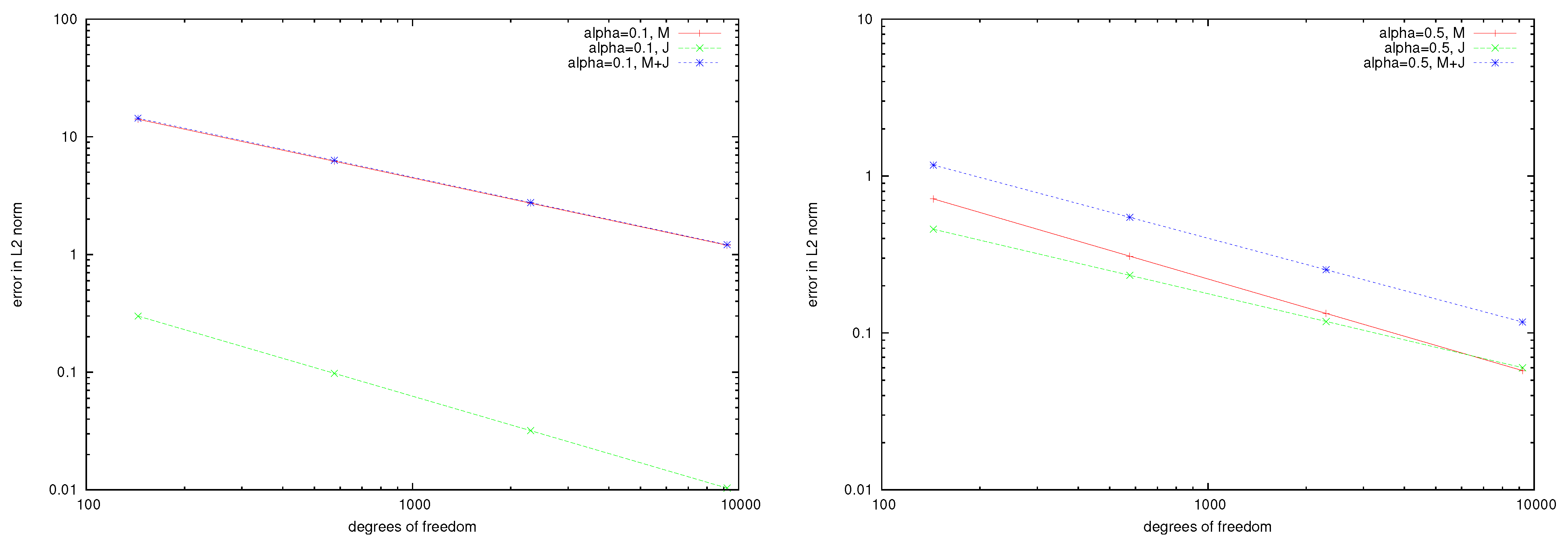
We used different values of $\alpha$ for our investigation. In Table 1, we present the results of the errors in energy norm and $L2$-norm for $\alpha =0.1,0.5,1.5$ for the uniform h version with polynomial degree $p=1$. In Figure 1 and Figure 2, we compare the h-version with different $\alpha$. The exact norm, known by extrapolation, for $\alpha =0.1$ is $\left|C\right|=8.580798$, for $\alpha =0.5$ is $\left|C\right|=1.6171534$, and for $\alpha =1.5$ is $\left|C\right|=1.8042380$. Here, $C=Re⟨{\mathbf{E}}_T^0,\mathbf{J}⟩$ and $C_h=Re⟨{\mathbf{E}}_T^0,{\mathbf{J}}_h⟩$ (see [27]). The exact $L2$-norms, known by extrapolation, for $\alpha =0.1$ are ${\parallel \mathbf{J}\parallel }_{L^2}=2.1066356$ and ${\parallel M\parallel }_{L^2}=81.9249906$; for $\alpha =0.5$ are ${\parallel \mathbf{J}\parallel }_{L^2}=2.1977966$ and ${\parallel M\parallel }_{L^2}=3.9588037$; and for $\alpha =1.5$ are ${\parallel \mathbf{J}\parallel }_{L^2}=2.3826646$ and ${\parallel M\parallel }_{L^2}=0.7763804$.

Table 1. Errors in $L^2$-norm and energy norm with respect to the degrees of freedom for $\alpha =0.1,0.5,1.5$.

N	DOF	$\left|\mathit{C}\right|$	$|\mathit{C}-{\mathit{C}}_{\mathit{h}}|$	${\parallel \mathit{J}\parallel }_{{\mathit{L}}^2}$	${\parallel \mathit{M}\parallel }_{{\mathit{L}}^2}$	${\parallel \mathit{J}-{\mathit{J}}_{\mathit{h}}\parallel }_{{\mathit{L}}^2}$	${\parallel \mathit{M}-{\mathit{M}}_{\mathit{h}}\parallel }_{{\mathit{L}}^2}$
				$\alpha =0.1$
1	144	8.502965	1.153119	2.085189	80.704374	0.299829	14.08929
2	576	8.568451	0.460150	2.104369	81.690279	0.097681	6.196968
3	2304	8.578833	0.033717	2.106395	81.879637	0.031823	2.725645
4	9216	8.654072	0.073274	2.117002	83.123825	0.010367	1.198835
				$\alpha =0.5$
1	144	1.603519	0.209552	2.149511	3.8937090	0.458159	0.714952
2	576	1.614451	0.093436	2.185426	3.9467491	0.232851	0.308704
3	2304	1.616616	0.041661	2.194608	3.9565591	0.118342	0.133293
4	9216	1.617260	0.018576	2.198619	3.9592220	0.060145	0.057554
				$\alpha =1.5$
1	144	1.774450	0.326497	2.350909	0.7243729	0.387707	0.279375
2	576	1.800799	0.111334	2.365011	0.7422644	0.343627	0.227618
3	2304	1.803838	0.037965	2.382843	0.7539064	0.304558	0.185450
4	9216	1.804284	0.012946	2.397906	0.7909461	0.269932	0.151093

Figure 1. Errors in the L2-norm for $\alpha =0.1,0.5$.

Figure 2. Errors in the L2-norm for $\alpha =1.5$ and the energy norm $|C-C_h|=O\left(h^{\eta }\right)$ for $\alpha =0.1,0.5,1.5$.

The convergence rates $\eta$, for $\alpha =0.1$ are, for the energy norm ${\eta }_C=1.325363$, and for the $L^2$-norm ${\eta }_{\mathbf{J}}=1.617988$ and ${\eta }_M=1.184964$. With $\alpha =0.5$, the energy norm of ${\eta }_C=1.165255$, the $L^2$-norms of ${\eta }_{\mathbf{J}}=0.976440$ and ${\eta }_M=1.211619$ and $\alpha =1.5$, for the energy norm ${\eta }_C=1.552163$, and for $L^2$-norm ${\eta }_{\mathbf{J}}=0.174124$ and ${\eta }_M=0.295586$.

Let us compare the numerical convergence rates above for the boundary element methods obtained in the above example with the theoretical convergence rates predicted by Theorem 1. Note that we have implemented the boundary integral equation system (26), and (27) and note the strongly elliptic system (30), where convergence is guaranteed due to Theorem 1. Nevertheless, our experiments show convergence for the boundary element solution, but with suboptimal convergence rates. Theorem 1 predicts (when Raviart–Thomas elements are used to approximate $\mathbf{J}$ and piecewise linear elements to approximate M) a convergence rate of order $\eta =\frac{3}{2}$ in the energy norm for smooth solutions $\mathbf{J}$ and M. Our computations depend on the parameter $\alpha$ which is a well-known effect with boundary integral equations where it may come to spurious eigenvalues diminishing the orders of the Galerkin approximations. Due to the cube ${\Omega }_{-}={[-2,2]}^3$, the numerical solution might become singular near the edges and corners of ${\Omega }_{-}$; hence, the Galerkin scheme converges sub-optimally.

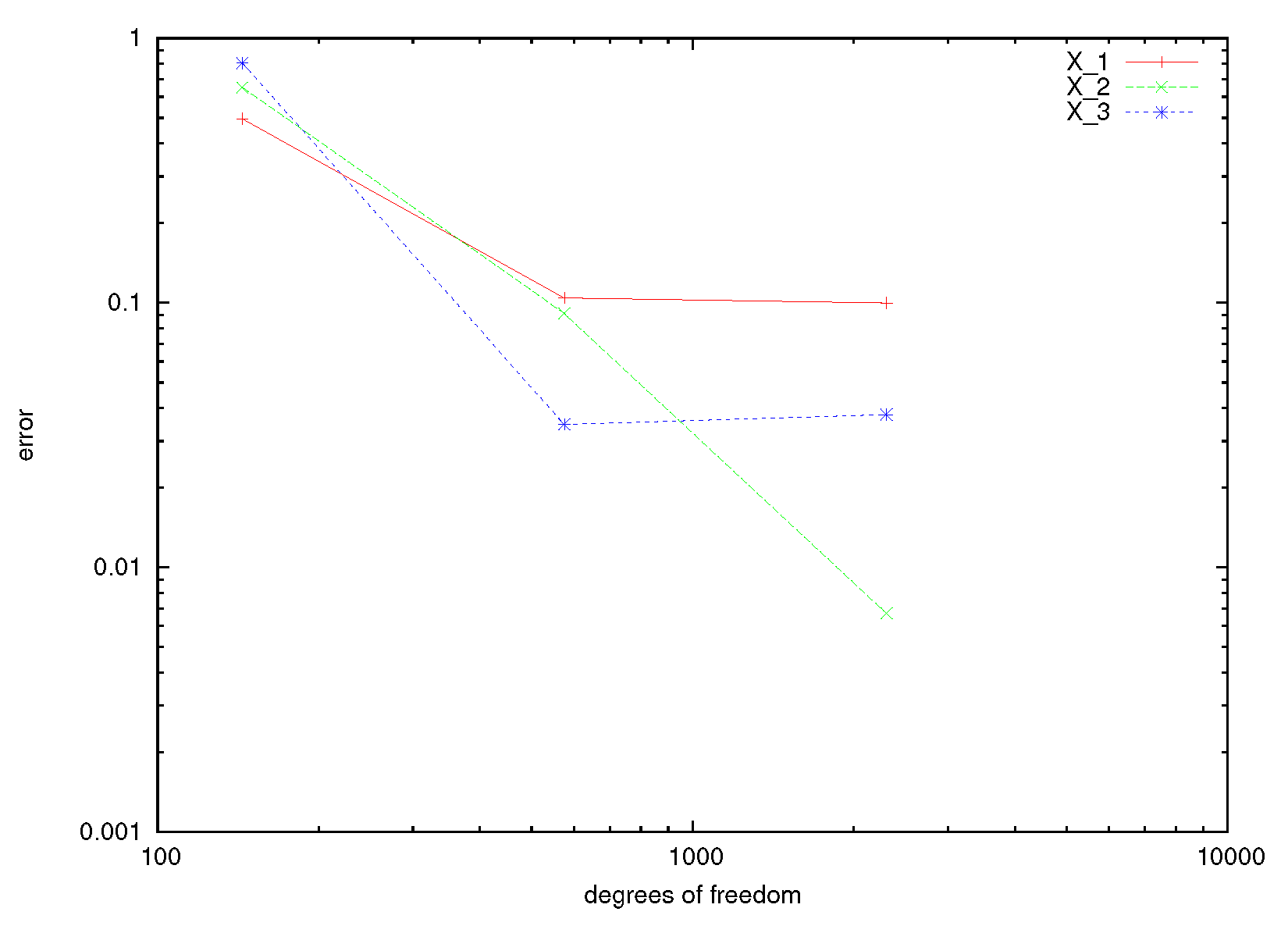
Next, we applied the boundary element method above to compute the first terms in the asymptotic expansion of the electrical field considered in Section 1 (Remark 1). In this way we obtained good results for the electrical field at some point away from the transmission surface $\Sigma$ by only computing a few terms in the expansion.

Algorithm for the asymptotic of the eddy current problem:

• First solve the exterior Problem $\left({\mathbf{P}}_{\alpha \infty }\right)$ by integral Equations (26) and (27), i.e., (35) with given incident field $-{\mathbf{E}}_T^0$.
• Compute ${\mathbf{H}}_T^{+}$ from (51).
• Go back to 1: Solve the exterior problem $\left({\mathbf{P}}_{\alpha \infty }\right)$ with new right hand side from (18).
• Go back to 2.
• $\mathbf{E}={\mathbf{E}}_0+{\beta }^{-1}{\mathbf{E}}_1+{\beta }^{-2}{\mathbf{E}}_2+{\mathbf{R}}_m$, where ${\mathbf{E}}_0$ is the solution of the step 1 and ${\mathbf{E}}_1$ and ${\mathbf{E}}_2$ are solutions of step 3.

We have $\tilde{\mathbf{E}}={\mathbf{E}}_0+{\beta }^{-1}{\mathbf{E}}_1+{\beta }^{-2}{\mathbf{E}}_2$, and calculate the error $|\tilde{\mathbf{E}}-{\mathbf{E}}_{\mathrm{exact}}\left({\mathbf{x}}_i\right)|$, $i=1,2,3$, where ${\mathbf{x}}_1=(3,0,0)$, ${\mathbf{x}}_2=(6,0,0)$ and ${\mathbf{x}}_3=(9,0,0)$. To find ${\mathbf{E}}_{\mathrm{exact}}$, Equations (25)–(53) are used. We present the results in Table 2 and in Figure 3.

Table 2. Errors for electrical field in ${\mathbf{x}}_1$, ${\mathbf{x}}_2$, and ${\mathbf{x}}_3$.

DOF	$|\tilde{\mathbf{E}}-{\mathbf{E}}_{\mathbf{exact}}\left({\mathbf{x}}_1\right)|$	$|\tilde{\mathbf{E}}-{\mathbf{E}}_{\mathbf{exact}}\left({\mathbf{x}}_2\right)|$	$|\tilde{\mathbf{E}}-{\mathbf{E}}_{\mathbf{exact}}\left({\mathbf{x}}_3\right)|$
144	0.4959	0.6499	0.8049
576	0.1043	0.0910	0.0347
2304	0.0998	0.0067	0.0378

Figure 3. Errors for the electrical field with respect to the degrees of freedom for ${\mathbf{x}}_1$, ${\mathbf{x}}_2$, and ${\mathbf{x}}_3$.

7. Conclusions

In this article we have studied the scattering of time-periodic electromagnetic fields by metallic obstacles, or the eddy current problem. An asymptotic procedure was described, applied for large conductivity, and reflects the skin effect in metals. A special integral equation procedure was introduced for the exterior boundary value problems corresponding to perfect conductors. In addition, an FEM/BEM coupling procedure was presented for the transmission problem, and the implementation of Galerkin’s elements was considered for the perfect conductor problem. The numerical experimentation showed good behavior by the procedure.