Highly Dispersive Optical Soliton Perturbation, with Maximum Intensity, for the Complex Ginzburg–Landau Equation by Semi-Inverse Variation

Abstract

This work analytically recovers the highly dispersive bright 1–soliton solution using for the perturbed complex Ginzburg–Landau equation, which is studied with three forms of nonlinear refractive index structures. They are Kerr law, parabolic law, and polynomial law. The perturbation terms appear with maximum allowable intensity, also known as full nonlinearity. The semi-inverse variational principle makes this retrieval possible. The amplitude–width relation is obtained by solving a cubic polynomial equation using Cardano’s approach. The parameter constraints for the existence of such solitons are also enumerated.

1. Introduction

One of the most important necessities with a mathematical model that describes soliton propagation across inter-continental distances is its integrability to secure an exact soliton solution. This provides the ease and convenience of conducting further analysis with such a solution structure at our disposal. Some such conveniences are the study of quasi-monochromatic solitons, the computing of the collision-induced timing jitter, the application of the variational principle, the implementation of the moment method approach, or even the application of collective variables to secure the dynamical system of soliton parameters [1,2,3,4,5,6,7,8,9,10,11,12,13,14,15,16,17,18,19,20,21,22,23,24,25,26,27,28,29,30]. Thus, it is necessary to recover the structure of a soliton. There are diverse approaches that can make this soliton solution retrieval possible. These range of approaches are visible in various works across the board. However, in specific situations, securing a soliton solution is rendered to be challenging. In fact, under such situations, the classic approach of inverse scattering transform is not applicable either, since the model fails the Painleve test of integrability. In such a situation, a modern approach of integrability has been successfully applied to recover an analytical bright 1–soliton solution. This is the application of the semi-inverse variational principle (SVP) that was proposed by J. H. He [11,12,17].

SVP was successfully implemented to a variety of problems in a wide range of physical situations. Apart from photonics, some such fields are fluid dynamics [2,9,10,12,13,23], relativistic quantum mechanics [21,24], plasma physics [4], mathematical chemistry [11], and various others [5,13,14,15,16,17,22,26]. In particular, the application of optics problems has been quite noticeably successful and widely visible, as reported [1,2,3,4,5,6,7,8,9,10,11,12,13,14,15,16,17,18,19,20]. The models that have been commonly studied in optics, with the implementation of SVP, are the Lakshmanan–Porsezian–Daniel model [1,7], Schrödinger’s nonlinear model [20], and the Fokas–Lenells model [8]. In this context, solitons were studied with chromatic dispersion [1] as well as cubic–quartic dispersive effects [7]. The novelty of the work ushers in with an established analytical soliton solution for an arbitrary maximum intensity where all pre-existing integration approaches fail.

The current paper will address SVP, for the first time, with the complex Ginzburg–Landau equation (CGLE) [3,19,25]. This will appear with six dispersion sources that constitute highly dispersive (HD) optical solitons [6,15,16,25]. The perturbation terms appear with maximum allowable intensity, i.e., AKA full nonlinearity [3,4,5,6,7,8,15,16,22]. Three forms of nonlinear refractive index structures are addressed: cubic (or Kerr) nonlinearity [1,3,14,25], parabolic (or cubic–quintic) nonlinearity [14,25], and polynomial nonlinearity [15,16,25]. Bright 1–soliton is finally extracted, for each law, where the soliton amplitude–width relation is recoverable by solving a cubic polynomial equation using Cardano’s approach [6]. The significance of the work is the retrieval of an analytical bright 1–soliton solution in spite of the fact that the perturbed CGLE is not rendered integrable by any of the pre-existing algorithms. The details are exhibited after introducing the model together with its perturbation terms.

Governing Model

The general form of CGLE without the perturbation terms reads as [25]

$$\begin{gathered} i{q}_t+i{a}_1{q}_x+a_2{q}_{xx}+i{a}_3{q}_{xxx}+a_4{q}_{xxxx}+i{a}_5{q}_{xxxxx} \\ +a_6{q}_{xxxxxx}+\frac{1}{{\left|q\right|}^2{q}^{*}}\left[\alpha {\left|q\right|}^2{\left({\left|q\right|}^2\right)}_{xx}-\beta {\left\{{\left({\left|q\right|}^2\right)}_x\right\}}^2\right]+F\left({\left|q\right|}^2\right)q=0. \end{gathered}$$

(1)

Here, $q\left(x,t\right)$ depicts the wave profile that travels down the optical fiber and is a complex valued function. The first term denotes the linear temporal evolution that has its coefficient as $i=\sqrt{-1}$. The coefficients of $a_j$ for $1\le j\le 6$ represent the six dispersion terms. Here, $a_1$ gives the inter-modal dispersion; $a_2$ accounts for the chromatic dispersion; while $a_3$ till $a_6$ yield the third-order, fourth-order, fifth-order, and sixth-order dispersion effects sequentially. Next, $\alpha$ and $\beta$ come from the nonlinear effects that are considered in CGLE [25]. The intensity-dependent nonlinear refractive index of the fiber is governed by the real valued functional $F$. The current paper will consider three nonlinear forms: cubic (or Kerr) nonlinearity, parabolic (or cubic–quintic) nonlinearity, and polynomial nonlinearity.

With perturbation terms turned on, the CGLE extends to

$$\begin{gathered} i{q}_t+i{a}_1{q}_x+a_2{q}_{xx}+i{a}_3{q}_{xxx}+a_4{q}_{xxxx}+i{a}_5{q}_{xxxxx} \\ +a_6{q}_{xxxxxx}+\frac{1}{{\left|q\right|}^2{q}^{*}}\left[\alpha {\left|q\right|}^2{\left({\left|q\right|}^2\right)}_{xx}-\beta {\left\{{\left({\left|q\right|}^2\right)}_x\right\}}^2\right]+F\left({\left|q\right|}^2\right)q \\ =i\left[\lambda {\left({\left|q\right|}^{2m}q\right)}_x+\theta {\left({\left|q\right|}^{2m}\right)}_{x}q+\sigma {\left|q\right|}^{2m}{q}_x\right]. \end{gathered}$$

(2)

The perturbation terms stem from the self-steepening effect, the self-frequency shift, and nonlinear dispersion, which are represented by the coefficients of $\lambda$, $\theta$, and $\sigma$, respectively. The parameter $m$ comes from maximum permissible intensity, also known as full nonlinearity.

2. Mathematical Start-Up

The starting hypothesis to handle Equation (2) is the substitution

$$q\left(x,t\right)=g\left(x-vt\right)e^{i\left(-\kappa x+\omega t+{\theta }_0\right)}=g\left(s\right)e^{i\left(-\kappa x+\omega t+{\theta }_0\right)}.$$

(3)

Here in (3), the function $g\left(x,t\right)$ is the traveling wave hypothesis while from the phase, $\omega$ is the wave number, while ${\theta }_0$ is the phase constant and $\kappa$ represents the frequency. Inserting (3) into (2) gives way to the following set of relations. The real part gives:

$$\begin{gathered} \left(-\omega -a_6{\kappa }^6+a_5{\kappa }^5+a_4{\kappa }^4-a_3{\kappa }^3-a_2{\kappa }^2+a_1\kappa \right)g \\ +\left(a_2+2\alpha +3a_3\kappa -6a_4{\kappa }^2-10a_5{\kappa }^3+15a_6{\kappa }^4\right)g^{″} \\ +\left(a_4+5a_5\kappa -15a_6{\kappa }^2\right)g^{\left(iv\right)}+a_6{g}^{\left(vi\right)}+2\left(\alpha -2\beta \right)\frac{{\left(g^{\prime }\right)}^2}{g} \\ +F\left(g^2\right)g=\kappa \left(\lambda +\sigma \right)g^{2m+1}. \end{gathered}$$

(4)

The imaginary part yields:

$$\begin{gathered} \left\{\left(2m+1\right)\lambda +2m\theta +\sigma \right\}{g}^{2m}{g}^{\prime } \\ +\left(v-a_1+2a_2\kappa +3a_3{\kappa }^2-4a_4{\kappa }^3-5a_5{\kappa }^4+6a_6{\kappa }^5\right)g^{\prime } \\ -\left(a_3-4a_4\kappa -10a_5{\kappa }^2+20a_6{\kappa }^3\right)g^{‴}-\left(a_5-6a_6\kappa \right)g^{\left(v\right)}=0. \end{gathered}$$

(5)

In (4) and (5), the notations $g^{\prime }=dg/ds$, $g^{″}=d^{2}g/d{s}^2$, $g^{‴}=d^{3}g/d{s}^3$, $g^{\left(iv\right)}=d^{4}g/d{s}^4$, $g^{\left(v\right)}=d^{5}g/d{s}^5$ and $g^{\left(vi\right)}=d^{6}g/d{s}^6$ are adopted. Next, introducing the parameters

$$P_1=-a_6{\kappa }^6+a_4{\kappa }^4+a_5{\kappa }^5-a_3{\kappa }^3-a_2{\kappa }^2+a_1\kappa -\omega ,$$

(6)

$$P_2=a_2+2\alpha +3a_3\kappa -6a_4{\kappa }^2-10a_5{\kappa }^3+15a_6{\kappa }^4,$$

(7)

$$P_3=a_4+5a_5\kappa -15a_6{\kappa }^2,$$

(8)

and setting

$$\alpha =2\beta ,$$

(9)

Equation (4) transforms to

$$P_{1}g+P_2{g}^{″}+P_3{g}^{\left(iv\right)}+a_6{g}^{\left(vi\right)}+F\left(g^2\right)g=\kappa \left(\lambda +\sigma \right)g^{2m+1}.$$

(10)

Thus, with (9), the governing Equation (2) modifies to:

$$\begin{gathered} i{q}_t+i{a}_1{q}_x+a_2{q}_{xx}+i{a}_3{q}_{xxx}+a_4{q}_{xxxx}+i{a}_5{q}_{xxxxx} \\ +a_6{q}_{xxxxxx}+\frac{\beta }{{\left|q\right|}^2{q}^{*}}\left[2{\left|q\right|}^2{\left({\left|q\right|}^2\right)}_{xx}-{\left\{{\left({\left|q\right|}^2\right)}_x\right\}}^2\right]+F\left({\left|q\right|}^2\right)q \\ =i\left[\lambda {\left({\left|q\right|}^{2m}q\right)}_x+\theta {\left({\left|q\right|}^{2m}\right)}_{x}q+\sigma {\left|q\right|}^{2m}{q}_x\right]. \end{gathered}$$

(11)

Next, the imaginary part Equation (5) gives the following parameter constraints

$$\left(2m+1\right)\lambda +2m\theta +\sigma =0,$$

(12)

$$v=a_1-2a_2\kappa -3a_3{\kappa }^2+4a_4{\kappa }^3+5a_5{\kappa }^4-6a_6{\kappa }^5,$$

(13)

$$a_3-4a_4\kappa -10a_5{\kappa }^2+20a_6{\kappa }^3=0,$$

(14)

and

$$a_5=6a_6\kappa .$$

(15)

Equation (13) gives the velocity. The relations (12)–(15) stay the same, irrespective of the type of nonlinearity considered.

3. Application of SVP

From Equation (10), multiplying by $g^{\prime }$ and integrating gives

$$\begin{gathered} P_1{g}^2+P_2{\left(g^{\prime }\right)}^2-P_3{\left(g^{″}\right)}^2+a_6{\left(g^{‴}\right)}^2 \\ +2\int F(g^2)g{g}^{\prime }dg-\frac{\kappa (\lambda +\sigma )}{m+1}{g}^{2m+2}=K, \end{gathered}$$

(16)

where $K$ is the integration constant. The stationary integral is introduced as below

$$J={\int }_{-\mathrm{\infty }}^{\mathrm{\infty }}\left[\begin{array}{c}{P}_1{g}^2+P_2{\left(g^{\prime }\right)}^2-P_3{\left(g^{″}\right)}^2+a_6{\left(g^{‴}\right)}^2\\ +2\int F\left(g^2\right)g{g}^{\prime }dg-\frac{\kappa (\lambda +\sigma )}{m+1}{g}^{2m+2}\hfill \end{array}\right]dx.$$

(17)

The bright 1–soliton to (11) is the same as that of the homogeneous counterpart, namely with $\lambda =\theta =\sigma =0$, whose structure is of the form:

$$g\left(s\right)=Af\left\{\sec \mathrm{h}B\left(x-vt\right)\right\},$$

(18)

where the functional form of the bright soliton, given by $f$, is based on the type of nonlinearity in question. The amplitude ($A$) and inverse width ($B$) of the soliton will be recovered by the coupled system of Equations (1)–(18):

$$\frac{\partial J}{\partial A}=0,$$

(19)

and

$$\frac{\partial J}{\partial B}=0.$$

(20)

This principle will be applied to study HD bright 1–soliton to (11) for three nonlinear forms.

3.1. Kerr Law

The refractive index structure is presented as

$$F\left(s\right)=b_{0}s,$$

(21)

where $b_0$ is a real-valued constant parameter. Thus, Equation (11) reads as

$$\begin{gathered} i{q}_t+i{a}_1{q}_x+a_2{q}_{xx}+i{a}_3{q}_{xxx}+a_4{q}_{xxxx}+i{a}_5{q}_{xxxxx} \\ +a_6{q}_{xxxxxx}+\frac{\beta }{{\left|q\right|}^2{q}^{*}}\left[2{\left|q\right|}^2{\left({\left|q\right|}^2\right)}_{xx}-{\left\{{\left({\left|q\right|}^2\right)}_x\right\}}^2\right]+b_0{\left|q\right|}^{2}q \\ =i\left[\lambda {\left({\left|q\right|}^{2m}q\right)}_x+\theta {\left({\left|q\right|}^{2m}\right)}_{x}q+\sigma {\left|q\right|}^{2m}{q}_x\right], \end{gathered}$$

(22)

so that (16) comes out as

$$2P_1{g}^2+2P_2{\left(g^{\prime }\right)}^2-2P_3{\left(g^{″}\right)}^2+2a_6{\left(g^{‴}\right)}^2+b_0{g}^4-\frac{2\kappa \left(\lambda +\sigma \right)}{m+1}{g}^{2m+2}=K.$$

(23)

The stationary integral, in this case, is introduced as

$$J={\int }_{-\mathrm{\infty }}^{\mathrm{\infty }}\left[\begin{array}{c}2P_1{g}^2+2P_2{\left(g^{\prime }\right)}^2-2P_3{\left(g^{″}\right)}^2\\ +2a_6{\left(g^{‴}\right)}^2+b_0{g}^4-\frac{2\kappa (\lambda +\sigma )}{m+1}{g}^{2m+2}\end{array}\right]dx.$$

(24)

The solution of (22), for $\lambda =\theta =\sigma =0$, is given as [19]

$$g\left(x-vt\right)=A{\sec \mathrm{h}}^3\left[B\left(x-vt\right)\right].$$

(25)

By substituting this 1–soliton solution into (24), one can obtain

$$\begin{gathered} J=\frac{16P_1}{15}\frac{A^2}{B}+\frac{144}{35}{P}_2{A}^{2}B-\frac{592}{35}{P}_3{A}^2{B}^3+\frac{15,024}{1155}{a}_6{A}^2{B}^5 \\ +\frac{256}{693}\frac{b_0{A}^4}{B}-\frac{\kappa \left(\lambda +\sigma \right)}{m+1}\frac{P{A}^{2m+2}}{B}, \end{gathered}$$

(26)

where

$$P=\frac{8m\left(3m+1\right)\left(3m+2\right)}{\left(2m+1\right)\left(6m+1\right)\left(6m+5\right)}\frac{\mathsf{\Gamma }\left(3m\right)\mathsf{\Gamma }\left(\frac{1}{2}\right)}{\mathsf{\Gamma }\left(3m+\frac{1}{2}\right)}.$$

(27)

The coupled pair of Equations (19) and (20), for Kerr law, is given as:

$$\frac{P_1}{15}+\frac{9}{35}{P}_2{B}^2-\frac{37}{35}{P}_3{B}^4+\frac{939}{1155}{a}_6{B}^6+\frac{32}{693}{b}_0{A}^2-\frac{\kappa \left(\lambda +\sigma \right)}{16}P{A}^{2m}=0,$$

(28)

and

$$-\frac{P_1}{15}+\frac{9}{35}{P}_2{B}^2-\frac{111}{35}{P}_3{B}^4+\frac{4695}{1155}{a}_6{B}^6+\frac{16}{693}{b}_0{A}^2-\frac{\kappa \left(\lambda +\sigma \right)}{16\left(m+1\right)}P{A}^{2m}=0.$$

(29)

Adding (28) and (29) leaves us with

$$\frac{18}{35}{P}_2{B}^2-\frac{148}{35}{P}_3{B}^4+\frac{5634}{1155}{a}_6{B}^6+\frac{48}{693}{b}_0{A}^2-\frac{\kappa \left(\lambda +\sigma \right)\left(m+2\right)}{16\left(m+1\right)}P{A}^{2m}=0.$$

(30)

Equation (30) can be restructured as a cubic polynomial equation in $u$:

$$a{u}^3+b{u}^2+cu+d=0,$$

(31)

with the following notations:

$$B^2=u,$$

(32)

$$a=\frac{5634}{1155}{a}_6,$$

(33)

$$b=-\frac{148}{35}{P}_3,$$

(34)

$$c=\frac{18}{35}{P}_2,$$

(35)

and

$$d=\frac{48}{693}{b}_0{A}^2-\frac{\kappa \left(\lambda +\sigma \right)\left(m+2\right)}{16\left(m+1\right)}P{A}^{2m}.$$

(36)

By Cardano’s method, (31) and (32) solves to [6]:

$$\begin{gathered} B=[{\left\{\left(-\frac{b^3}{27a^3}+\frac{bc}{6a^2}-\frac{d}{2a}\right)-\sqrt{{\left(-\frac{b^3}{27a^3}+\frac{bc}{6a^2}-\frac{d}{2a}\right)}^2+{\left(\frac{c}{3a}-\frac{b^2}{9a^2}\right)}^3}\right\}}^{\frac{1}{3}} \\ +{{\left\{\left(-\frac{b^3}{27a^3}+\frac{bc}{6a^2}-\frac{d}{2a}\right)+\sqrt{{\left(-\frac{b^3}{27a^3}+\frac{bc}{6a^2}-\frac{d}{2a}\right)}^2+{\left(\frac{c}{3a}-\frac{b^2}{9a^2}\right)}^3}\right\}}^{\frac{1}{3}}-\frac{b}{3a}]}^{\frac{1}{2}}. \end{gathered}$$

(37)

The constraint for this solution to exist is

$$a_6\ne 0,$$

(38)

along with the discriminant

$${\left(-\frac{b^3}{27a^3}+\frac{bc}{6a^2}-\frac{d}{2a}\right)}^2+{\left(\frac{c}{3a}-\frac{b^2}{9a^2}\right)}^3>0.$$

(39)

Moreover,

$$\begin{gathered} {\left\{\left(-\frac{d}{2a}+\frac{bc}{6a^2}-\frac{b^3}{27a^3}\right)-\sqrt{{\left(-\frac{d}{2a}+\frac{bc}{6a^2}-\frac{b^3}{27a^3}\right)}^2+{\left(\frac{c}{3a}-\frac{b^2}{9a^2}\right)}^3}\right\}}^{\frac{1}{3}} \\ +{\left\{\left(-\frac{d}{2a}+\frac{bc}{6a^2}-\frac{b^3}{27a^3}\right)+\sqrt{{\left(-\frac{d}{2a}+\frac{bc}{6a^2}-\frac{b^3}{27a^3}\right)}^2+{\left(\frac{c}{3a}-\frac{b^2}{9a^2}\right)}^3}\right\}}^{\frac{1}{3}}>\frac{b}{3a}. \end{gathered}$$

(40)

Thus, the HD bright 1–soliton to (22) is introduced as (see Figure 1)

$$q\left(x,t\right)=A{\sec \mathrm{h}}^3\left[B\left(x-vt\right)\right]e^{i\left(-\kappa x+\omega t+{\theta }_0\right)}.$$

(41)

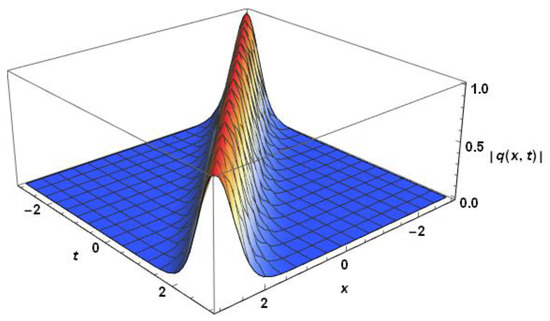
Figure 1. Profile of the HD bright 1–soliton (41) setting all arbitrary parameters to unity.

Here, the inverse width $\left(B\right)$ is explicitly expressed via (37), provided that the constraint conditions given by (38)–(40) are maintained.

3.2. Parabolic Law

The refractive index structure is indicated below

$$F\left(s\right)=b_{1}s+b_2{s}^2,$$

(42)

where $b_1$ and $b_2$ are real-valued constant parameters. Then, Equation (11) evolves as

$$\begin{gathered} i{q}_t+i{a}_1{q}_x+a_2{q}_{xx}+i{a}_3{q}_{xxx}+a_4{q}_{xxxx}+i{a}_5{q}_{xxxxx} \\ +a_6{q}_{xxxxxx}+\frac{\beta }{{\left|q\right|}^2{q}^{*}}\left[2{\left|q\right|}^2{\left({\left|q\right|}^2\right)}_{xx}-{\left\{{\left({\left|q\right|}^2\right)}_x\right\}}^2\right]+\left(b_1{\left|q\right|}^2+b_2{\left|q\right|}^4\right)q \\ =i\left[\lambda {\left({\left|q\right|}^{2m}q\right)}_x+\theta {\left({\left|q\right|}^{2m}\right)}_{x}q+\sigma {\left|q\right|}^{2m}{q}_x\right], \end{gathered}$$

(43)

so that (16) comes out as

$$\begin{gathered} 6P_1{g}^2+6P_2{\left(g^{\prime }\right)}^2-6P_3{\left(g^{″}\right)}^2+6a_6{\left(g^{‴}\right)}^2 \\ +3b_1{g}^4+2b_2{g}^6-\frac{6\kappa (\lambda +\sigma )}{m+1}{g}^{2m+2}=K. \end{gathered}$$

(44)

The stationary integral, in this case, is structured as

$$J={\int }_{-\mathrm{\infty }}^{\mathrm{\infty }}\left[\begin{array}{c}6P_1{g}^2+6P_2{\left(g^{\prime }\right)}^2-6P_3{\left(g^{″}\right)}^2+6a_6{\left(g^{‴}\right)}^2\\ +3b_1{g}^4+2b_2{g}^6-\frac{6\kappa (\lambda +\sigma )}{m+1}{g}^{2m+2}\end{array}\right]dx.$$

(45)

The solution of (43), for $\lambda =\theta =\sigma =0$, is given as [19]

$$g\left(x-vt\right)=A{\sec \mathrm{h}}^{\frac{3}{2}}\left[B\left(x-vt\right)\right].$$

(46)

Byubstituting this 1–soliton solution into (45), one can obtain

$$\begin{gathered} J=\pi P_1\frac{A^2}{B}+\frac{9\pi }{16}{P}_2{A}^{2}B-\frac{153}{128}{P}_3{A}^2{B}^3+\frac{\mathrm{21,429}}{4096}{a}_6{A}^2{B}^5 \\ +\frac{16}{15}\frac{b_1{A}^4}{B}+\frac{35\pi }{192}\frac{b_2{A}^6}{B}-\frac{6\kappa (\lambda +\sigma )P}{m+1}\frac{A^{2m+2}}{B}, \end{gathered}$$

(47)

where

$$P=\frac{2\left(3m+1\right)}{3m\left(3m+2\right)}\frac{\mathsf{\Gamma }\left(\frac{3m}{2}+\frac{1}{2}\right)\mathsf{\Gamma }\left(\frac{1}{2}\right)}{\mathsf{\Gamma }\left(\frac{3m}{2}\right)}.$$

(48)

The coupled pair of Equations (19) and (20), for parabolic law, is:

$$\begin{gathered} \pi P_1+\frac{9\pi }{16}{P}_2{B}^2-\frac{153\pi }{128}{P}_3{B}^4+\frac{\mathrm{21,429}\pi }{4096}{a}_6{B}^6 \\ +\frac{32}{15}{b}_1{A}^2+\frac{35\pi }{64}{b}_2{A}^4-2\kappa \left(\lambda +\sigma \right)P{A}^{2m}=0, \end{gathered}$$

(49)

and

$$\begin{gathered} -\pi P_1+\frac{9\pi }{16}{P}_2{B}^2-\frac{459\pi }{128}{P}_3{B}^4+\frac{\mathrm{107,145}\pi }{4096}{a}_6{B}^6 \\ -\frac{16}{15}{b}_1{A}^2-\frac{35\pi }{192}{b}_2{A}^4+\frac{2\kappa \left(\lambda +\sigma \right)}{m+1}P{A}^{2m}=0. \end{gathered}$$

(50)

Adding (49) and (50) yields

$$\begin{gathered} \frac{9\pi }{8}{P}_2{B}^2-\frac{153\pi }{32}{P}_3{B}^4+\frac{\mathrm{64,287}\pi }{2048}{a}_6{B}^6 \\ +\frac{16}{15}{b}_1{A}^2+\frac{70\pi }{192}{b}_2{A}^4-\frac{2m\kappa \left(\lambda +\sigma \right)}{m+1}P{A}^{2m}=0. \end{gathered}$$

(51)

Equation (51) is reducible to (31) with

$$a=\frac{\mathrm{64,287}\pi }{2048}{a}_6,$$

(52)

$$b=-\frac{153\pi }{32}{P}_3,$$

(53)

$$c=\frac{9\pi }{8}{P}_2,$$

(54)

and

$$d=\frac{16}{15}{b}_1{A}^2+\frac{70\pi }{192}{b}_2{A}^4-\frac{2m\kappa \left(\lambda +\sigma \right)}{m+1}P{A}^{2m}.$$

(55)

Hence, the HD bright 1–soliton to (43) reads as (see Figure 2)

$$q\left(x,t\right)=A{\sec \mathrm{h}}^{\frac{3}{2}}\left[B\left(x-vt\right)\right]e^{i\left(-\kappa x+\omega t+{\theta }_0\right)}.$$

(56)

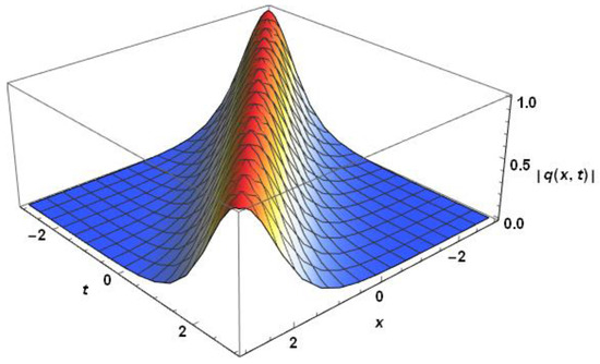
Figure 2. Profile of the HD bright 1–soliton (56) setting all arbitrary parameters to unity.

Here, the inverse width $\left(B\right)$ is explicitly expressed via (37), providing that the constraint conditions given by (38)–(40) are maintained.

3.3. Polynomial Law

The refractive index structure extends to

$$F\left(s\right)=b_{1}s+b_2{s}^2+b_3{s}^3,$$

(57)

where $b_1$, $b_2$, and are real-valued constant parameters. Hence, Equation (11) comes out as

$$\begin{gathered} i{q}_t+i{a}_1{q}_x+a_2{q}_{xx}+i{a}_3{q}_{xxx}+a_4{q}_{xxxx}+i{a}_5{q}_{xxxxx}+a_6{q}_{xxxxxx} \\ +\left(b_1{\left|q\right|}^2+b_2{\left|q\right|}^4+b_3{\left|q\right|}^6\right)q+\frac{\beta }{{\left|q\right|}^2{q}^{*}}\left[2{\left|q\right|}^2{\left({\left|q\right|}^2\right)}_{xx}-{\left\{{\left({\left|q\right|}^2\right)}_x\right\}}^2\right] \\ =i\left[\lambda {\left({\left|q\right|}^{2m}q\right)}_x+\theta {\left({\left|q\right|}^{2m}\right)}_{x}q+\sigma {\left|q\right|}^{2m}{q}_x\right], \end{gathered}$$

(58)

so that (16) now is

$$\begin{gathered} 12P_1{g}^2+12P_2{\left(g^{\prime }\right)}^2-12P_3{\left(g^{″}\right)}^2+12a_6{\left(g^{‴}\right)}^2 \\ +6b_1{g}^4+4b_2{g}^6+3b_3{g}^8-\frac{12\kappa \left(\lambda +\sigma \right)}{m+1}{g}^{2m+2}=K. \end{gathered}$$

(59)

The stationary integral, for polynomial law, reads as

$$J={\int }_{-\mathrm{\infty }}^{\mathrm{\infty }}\left[\begin{array}{c}12P_1{g}^2+12P_2{\left(g^{\prime }\right)}^2-12P_3{\left(g^{″}\right)}^2+12a_6{\left(g^{‴}\right)}^2\\ +6b_1{g}^4+4b_2{g}^6+3b_3{g}^8-\frac{12\kappa (\lambda +\sigma )}{m+1}{g}^{2m+2}\hfill \end{array}\right]dx.$$

(60)

The solution of (58), for $\lambda =\theta =\sigma =0$, is [19]

$$g\left(x-vt\right)=A\sec \mathrm{h}\left[B\left(x-vt\right)\right].$$

(61)

By substituting this 1–soliton solution into (60), one can obtain

$$\begin{gathered} J=3P_1\frac{A^2}{B}+P_2{A}^{2}B-\frac{7}{5}{P}_3{A}^2{B}^3+\frac{31}{7}{a}_6{A}^2{B}^5+\frac{b_1{A}^4}{B} \\ +\frac{8b_2}{15}\frac{A^6}{B}+\frac{12b_3}{35}\frac{A^8}{B}-\frac{3\kappa \left(\lambda +\sigma \right)P}{m+1}\frac{A^{2m+2}}{B}, \end{gathered}$$

(62)

where

$$P=\frac{m}{2m+1}\frac{\mathsf{\Gamma }\left(m\right)\mathsf{\Gamma }\left(\frac{1}{2}\right)}{\mathsf{\Gamma }\left(m+\frac{1}{2}\right)}.$$

(63)

The coupled pair of Equations (19) and (20), for polynomial law, formulates as:

$$\begin{gathered} 3P_1+P_2{B}^2-\frac{7}{5}{P}_3{B}^4+\frac{31}{7}{a}_6{B}^6+2b_1{A}^2 \\ +\frac{24}{15}{b}_2{A}^4+\frac{48}{35}{b}_3{A}^6-3\kappa \left(\lambda +\sigma \right)P{A}^{2m}=0, \end{gathered}$$

(64)

and

$$\begin{gathered} -3P_1+P_2{B}^2-\frac{21}{5}{P}_3{B}^4+\frac{155}{7}{a}_6{B}^6-b_1{A}^2 \\ -\frac{8}{15}{b}_2{A}^4-\frac{12}{35}{b}_3{A}^6-\frac{3\kappa \left(\lambda +\sigma \right)}{m+1}P{A}^{2m}=0. \end{gathered}$$

(65)

Adding (64) and (65) implies to

$$\begin{gathered} 2P_2{B}^2-\frac{28}{5}{P}_3{B}^4+\frac{186}{7}{a}_6{B}^6+b_1{A}^2+\frac{16}{15}{b}_2{A}^4 \\ +\frac{36}{35}{b}_3{A}^6-\frac{3\left(m+2\right)\kappa \left(\lambda +\sigma \right)}{m+1}P{A}^{2m}=0. \end{gathered}$$

(66)

Again, Equation (66) is transformable to the cubic polynomial Equation (31) where

$$a=\frac{186}{7}{a}_6,$$

(67)

$$b=-\frac{28}{5}{P}_3,$$

(68)

$$c=2P_2,$$

(69)

and

$$d=b_1{A}^2+\frac{16}{15}{b}_2{A}^4+\frac{36}{35}{b}_3{A}^6-\frac{3\left(m+2\right)\kappa \left(\lambda +\sigma \right)}{m+1}P{A}^{2m}.$$

(70)

Hence, the HD bright 1–soliton to (58) comes out as (see Figure 3)

$$q\left(x,t\right)=A\sec \mathrm{h}\left[B\left(x-vt\right)\right]e^{i\left(-\kappa x+\omega t+{\theta }_0\right)}.$$

(71)

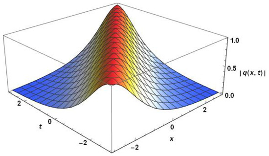
Figure 3. Profile of the HD bright 1–soliton (71) setting all arbitrary parameters to unity.

Here, the inverse width ($B$) is explicitly expressed via (37), providing that the constraint conditions given by (38)–(40) are maintained.

4. Conclusions

This work obtains an analytical expression of the HD bright 1–soliton to the perturbed CGLE by SVP, where the perturbation terms are considered with the maximum allowable intensity. Three nonlinear forms are addressed. Such an analytical 1–soliton solution, with arbitrary intensity parameters, in its closed form, and is not recoverable by any of the pre-existing integration algorithms.

There are some shortcomings to this approach. It is only the bright soliton that is obtainable using this approach. This scheme fails to retrieve singular or dark solitons since the stationary integral is rendered to be divergent with singular or dark solitons. The bright 1–soliton solutions that are recovered for three nonlinear forms are not exact since they are obtained by the usage of a principle, namely the SVP. Therefore, the results of this work cannot be compared with any pre-existing results since there are none. The homogenous model was first proposed during 2021 [25] and the current paper is the very first one to extend the model with perturbation terms and with full nonlinearity. The simulations, therefore, provide a visual accuracy to the proposed approach, namely the SVP.

This analytical soliton solution can take us further along with advanced studies. Some of them include the analysis of quasi-monochromatic solitons, the computing of the soliton parameter dynamics with the help of the variational principle, the study of the collision-induced timing jitter and the numerical simulation of the problem with the application of the Adomian decomposition algorithm, Laplace ADM, and variational iteration approach. More research results that can be aligned with the current findings [27,28,29,30] exist.

References

- Alqahtani, R.T.; Babatin, M.M.; Biswas, A. Bright optical solitons for Lakshmanan–Porsezian–Daniel model by semi–inverse variational principle. Optik 2018, 154, 109–114. [Google Scholar] [CrossRef]
- Biswas, A.; Milovic, D.; Kumar, S.; Yildirim, A. Perturbation of shallow water waves by semi–inverse variational principle. Indian J. Phys. 2013, 87, 567–569. [Google Scholar] [CrossRef]
- Biswas, A.; Alqahtani, R.T. Optical soliton perturbation with complex Ginzburg–Landau equation by semi–inverse variational principle. Optik 2017, 147, 77–81. [Google Scholar] [CrossRef]
- Biswas, A.; Alqahtani, R.T. Chirp–free bright optical solitons for perturbed Gerdjikov–Ivanov equation by semi–inverse variational principle. Optik 2017, 147, 72–76. [Google Scholar] [CrossRef]
- Biswas, A.; Asma, M.; Guggilla, P.; Mullick, L.; Moraru, L.; Ekici, M.; Alzahrani, A.K.; Belic, M.R. Optical soliton perturbation with Kudryashov’s equation by semi–inverse variational principle. Phys. Lett. A 2020, 384, 126830. [Google Scholar] [CrossRef]
- Biswas, A.; Ekici, M.; Dakova, A.; Khan, S.; Moshokoa, S.P.; Alshehri, H.M.; Belic, M.R. Highly dispersive optical soliton perturbation with Kudryashov’s sextic–power law nonlinear refractive index by semi–inverse variation. Results Phys. 2021, 27, 104539. [Google Scholar] [CrossRef]
- Biswas, A.; Edoki, J.; Guggilla, P.; Khan, S.; Alzahrani, A.K.; Belic, M.R. Cubic–quartic optical soliton perturbation with Lakshmanan–Porsezian–Daniel model by semi–inverse variational principle. Ukr. J. Phys. Opt. 2021, 22, 122–127. [Google Scholar] [CrossRef]
- Biswas, A.; Dakova, A.; Khan, S.; Ekici, M.; Moraru, L.; Belic, M.R. Cubic–quartic optical soliton perturbation with Fokas–Lenells equation by semi–inverse variation. Semicond. Phys. Quantum Electron. Optoelectron. 2021, 24, 431–435. [Google Scholar] [CrossRef]
- Collins, T.; Kara, A.H.; Bhrawy, A.H.; Triki, H.; Biswas, A. Dynamics of shallow water waves with logarithmic nonlinearity. Rom. Rep. Phys. 2016, 68, 943–961. [Google Scholar]
- Girgis, L.; Biswas, A. A study of solitary waves by He’s variational principle. Wave Random Complex. 2011, 21, 96–104. [Google Scholar] [CrossRef]
- He, J.H. Semi-inverse method and generalized variational principles with multi-variables in elasticity. Appl. Math. Mech. 2000, 21, 797–808. [Google Scholar]
- He, J.H. Variational principle and periodic solution of the Kundu–Mukherjee–Naskar equation. Results Phys. 2020, 17, 103031. [Google Scholar] [CrossRef]
- Kheir, H.; Jabbari, A.; Yildirim, A.; Alomari, A.K. He’s semi–inverse method for soliton solutions of Boussinesq system. World J. Model. Simul. 2013, 9, 3–13. [Google Scholar]
- Kohl, R.; Milovic, D.; Zerrad, E.; Biswas, A. Optical solitons by He’s variational principle in a non–Kerr law media. J. Infrared Millim. Terahertz Waves 2009, 30, 526–537. [Google Scholar] [CrossRef]
- Kohl, R.W.; Biswas, A.; Ekici, M.; Zhou, Q.; Khan, S.; Alshomrani, A.S.; Belic, M.R. Highly dispersive optical soliton perturbation with cubic–quintic–septic refractive index by semi–inverse variational principle. Optik 2019, 199, 163322. [Google Scholar] [CrossRef]
- Kohl, R.W.; Biswas, A.; Ekici, M.; Zhou, Q.; Khan, S.; Alshomrani, A.S.; Belic, M.R. Sequel to highly dispersive optical soliton perturbation with cubic–quintic–septic refractive index by semi–inverse variational principle. Optik 2020, 203, 163451. [Google Scholar] [CrossRef]
- Li, X.W.; Li, Y.; He, J.H. On the semi–inverse method and variational principle. Therm. Sci. 2013, 17, 1565–1568. [Google Scholar] [CrossRef]
- Liu, H.M. The variational principle for Yang–Mills equation by semi–inverse method. Facta Univ. Ser. Mech. Autom. Control Robot. 2004, 4, 169–171. [Google Scholar]
- Liu, W.Y.; Yu, Y.J.; Chen, L.D. Variational principles for Ginzburg–Landau equation by He’s semi–inverse method. Chaos Solit. Fractals 2007, 33, 1801–1803. [Google Scholar] [CrossRef]
- Ozis, T.; Yildirim, A. Application of He’s semi–inverse method to the nonlinear Schrodinger equation. Comput. Math. Appl. 2007, 54, 1039–1042. [Google Scholar] [CrossRef]
- Sassaman, R.; Heidari, A.; Biswas, A. Topological and non–topological solitons of nonlinear Klein–Gordon equations by He’s semi–inverse variational porinciple. J. Franklin Inst. 2010, 347, 1148–1157. [Google Scholar] [CrossRef]
- Singh, S.S. Bright and dark 1–soliton solutions to perturbed Schrodinger–Hirota equation with power law nonlinearity via semi–inverse variation method and ansatz method. Int. J. Phys. Res. 2017, 5, 39–42. [Google Scholar] [CrossRef]
- Tao, Z.L. Solving the breaking soliton equation by He’s variational method. Comput. Math. Appl. 2009, 58, 2395–2397. [Google Scholar] [CrossRef][Green Version]
- Yan, W.; Liu, Q.; Zhu, C.M.; Zhao, Y.; Shi, Y. Semi–inverse method to the Klein–Gordon equation with quadratic nonlinearity. Appl. Comput. Electromagn. Soc. J. 2018, 33, 842–846. [Google Scholar]
- Zayed, E.M.E.; Gepreel, K.A.; El–Horbaty, M.; Biswas, A.; Yildirim, Y.; Alshehri, H.M. Highly dispersive optical solitons with complex Ginzburg–Landau equation having six nonlinear forms. Mathematics 2021, 9, 3270. [Google Scholar] [CrossRef]
- Zhang, J.; Yu, J.Y.; Pan, N. Variational principles for nonlinear fiber optics. Chaos Solit. Fractals 2005, 24, 309–311. [Google Scholar] [CrossRef]
- Abdel–Gawad, H.I. Chirped, breathers, diamond and W-shaped optical waves propagation in nonself–phase modulation medium. Biswas–Arshed equation. Int. J. Mod. Phys. B 2017, 35, 2150097. [Google Scholar] [CrossRef]
- Abdel–Gawad, H.I. A generalized Kundu–Eckhaus equation with an extra–dispersion: Pulses configuration. Opt. Quantum Electron. 2021, 53, 705. [Google Scholar] [CrossRef]
- Abdel–Gawad, H.I. Study of modulation instability and geometric structures of multisolitons in a medium with high dispersivity and nonlinearity. Pramana 2021, 95, 146. [Google Scholar] [CrossRef]
- Tantawy, M.; Abdel–Gawad, H.I. On multi–geometric structures optical waves propagation in self–phase modulation medium: Sasa–Satsuma equation. Eur. Phys. J. Plus 2020, 135, 928. [Google Scholar] [CrossRef]
Publisher’s Note: MDPI stays neutral with regard to jurisdictional claims in published maps and institutional affiliations. |
© 2022 by the authors. Licensee MDPI, Basel, Switzerland. This article is an open access article distributed under the terms and conditions of the Creative Commons Attribution (CC BY) license (https://creativecommons.org/licenses/by/4.0/).