T-Spherical Fuzzy Bonferroni Mean Operators and Their Application in Multiple Attribute Decision Making

Abstract

To deal with complicated decision problems with T-Spherical fuzzy values in the aggregation process, T-Spherical fuzzy Bonferroni mean operators are developed by extending the Bonferroni mean and Dombi mean to a T-Spherical fuzzy environment. The T-spherical fuzzy interaction Bonferroni mean operator and the T-spherical fuzzy interaction geometric Bonferroni mean operator are first defined. Then, the T-spherical fuzzy interaction weighted Bonferroni mean operator and the T-spherical fuzzy weighted interaction geometric Bonferroni mean operator are defined. Based on the Dombi mean and the Bonferroni mean operator, some T-Spherical fuzzy Dombi Bonferroni mean operators are proposed, including the T-spherical fuzzy Dombi Bonferroni mean operator, T-spherical fuzzy geometric Dombi Bonferroni mean operator, T-spherical fuzzy weighted Dombi Bonferroni mean operator and the T-spherical fuzzy weighted geometric Dombi Bonferroni mean operator. The properties of these proposed operators are studied. An attribute weight determining method based on the T-spherical fuzzy entropy and symmetric T-spherical fuzzy cross-entropy is developed. A new decision making method based on the proposed T-Spherical fuzzy Bonferroni mean operators is proposed for partly known or completely unknown attribute weight situations. The furniture procurement problem is presented to illustrate the new algorithm, and some comparisons are made.

1. Introduction

Decision problems with fuzzy and uncertain information exist extensively in the real decision making process since decision problems become increasingly complicated. Many useful tools have been developed to model these information, among which Spherical fuzzy sets is an important one developed by Ashraf et al. [1] by extending picture fuzzy sets and intuitionistic fuzzy sets [2,3]. Spherical fuzzy sets have been studied and extended extensively [4,5].

Ashraf and Abdullah [6] developed generalized spherical aggregation operators based on the Archimedean t-norm and t-conorm. Donyatalab et al. [7] defined a spherical fuzzy weighted mean operator and Spherical Fuzzy Einstein weighted Harmonic mean operator. T-spherical fuzzy sets were proposed by Mahmood et al. [8] to generalize Spherical fuzzy sets. Zeng et al. [9] proposed some Einstein geometric averaging interactive aggregation operators.

Zeng et al. [10] introduced T-spherical fuzzy interactive aggregation operators with associate probability. Al-Quran [11] proposed T-spherical hesitant fuzzy sets by combining the hesitant fuzzy and the T-spherical hesitant fuzzy set. Some T-spherical hesitant fuzzy weighted averaging operators have been defined, including the T-spherical hesitant fuzzy weighted averaging operator and the T-spherical hesitant fuzzy weighted geometric operator in [11].

Jan et al. [12] developed the T-spherical fuzzy graph concept and dominant theory of T-spherical fuzzy graphs. Munir et al. [13] defined some Einstein operations based on the Einstein t-norms and t-conorms for T-spherical fuzzy set and developed some T-spherical fuzzy Einstein geometric averaging aggregation operators. Ju et al. [14] extended the TODIM method to the T-spherical fuzzy environment. Xian et al. [15] applied the T-spherical fuzzy c-means method to image segmentation.

Zedam et al. [16] defined the T-spherical fuzzy graph and some related concepts, including subgraphs, the shortest path etc. Guleria and Bajaj [17] applied the T-spherical fuzzy graph notion for supply chain management problems. Mahmood et al. [18] developed T-spherical fuzzy MULTIMOORA method and T-spherical fuzzy Dombi prioritized aggregation operators. Munir et al. [19] introduced some T-spherical fuzzy interactive geometric operators with immediate probability information.

Liu et al. [20] proposed a decision making method based on the T-spherical fuzzy generalized Maclaurin symmetric mean operator and applied it into the problem of selecting the Yunnan Baiyao’s R&D project. Wang and Chen [21] presented the T-spherical fuzzy ELECTRE approach by incorporating two forms of Minkowski distance measures. T-spherical fuzzy correlation coefficients [22] and T-spherical fuzzy similarity measures [23] have been studied, and their applications in clustering were presented.

Khan et al. [24] studied T-spherical fuzzy Schweizer–Sklar weighted geometric Heronian mean operator. Garg et al. [25] proposed the T-spherical fuzzy interactive geometric operators. Mahmood et al. [26] defined interval-valued T-spherical fuzzy soft sets and developed some interval-valued T-spherical fuzzy soft aggregation operators. Garg et al. [27] developed T-spherical fuzzy power aggregation operators.

Ullah et al. [28] defined some T-spherical fuzzy Hamacher aggregation operators. Based on the T-spherical fuzzy values, some new fuzzy sets have been defined and studied [29,30,31,32,33,34,35,36]. Chen et al. [32] presented generalized T-spherical fuzzy geometric aggregation operators; however, the interaction of the operation laws has not been considered.

Though many T-spherical fuzzy multiple attribute decision making methods have been proposed, there are still many decision making problems that cannot be solved using existing methods. Aggregation operators are important in decision making process [36], we develop some new T-spherical fuzzy aggregation operators based on the Bonferroni mean operator and Dombi operator in this paper.

The Bonferroni mean operator is the product of each input value with the average one of the other input values [37,38]. The Bonferroni mean operator has been extended extensively. The Bonferroni geometric mean operator has been studied by Xia et al. [39] and Li et al. [40]. Zhu and Xu [41] developed the hesitant fuzzy Bonferroni mean operator. Zhu et al. [42] studied the hesitant fuzzy geometric Bonferroni mean operator.

He et al. [43] developed the intuitionistic fuzzy geometric power Bonferroni means operators by combing the geometric Bonferroni mean operator with the power mean operator. Park et al. [44] studied optimized weighted geometric Bonferroni means for intuitionistic fuzzy information. Wei et al. [45] proposed the uncertain linguistic Bonferroni mean operators. Liu and Liu [46] defined the intuitionistic uncertain linguistic partitioned Bonferroni mean operators. Chen et al. [47] developed the linguistic 2-tuple geometric Bonferroni mean operator.

Yang et al. [48] studied hesitant Pythagorean fuzzy geometric weight Bonferroni mean operator considering interactions between arguments. Yang et al. [49] studied Pythagorean fuzzy partitioned Bonferroni mean considering interactions. Yang and Pang [50] studied fuzzy Bonferroni mean Dombi aggregation operators in q-rung orthopair fuzzy environments.

Liu and Liu [51] defined normal intuitionistic fuzzy Bonferroni mean operators. Mesiarova-Zemankova et al. [52] introduced the weighted Bonferroni mean considering interactions between inputs. Liang et al. [53] presented interval-valued Pythagorean fuzzy Bonferroni mean operators. Ate and Akay [54] developed picture fuzzy Bonferroni mean operators.

Mahmood and Ahsen [55] presented some picture-hesitant fuzzy Bonferroni mean operators. Although the Bonferroni mean operator has been extended into various environments, the Bonferroni mean operator in T-spherical fuzzy environments has not been studied. Hence, we extend the Bonferroni mean operator to the T-spherical fuzzy environment considering the interaction operations between T-spherical fuzzy values.

The Dombi mean [56] is a flexible aggregation method by a parameter that is based on the Dombi t-norm and Dombi t-conorm. The Dombi aggregation has also received extensive attention. Liu et al. [57] studied Pythagorean fuzzy Dombi power average operators. Jana and Pal [58] presented single-valued neutrosophic aggregation operators.

Wu et al. [59] proposed Dombi Hamy mean operators in interval-valued intuitionistic fuzzy environments. Jana et al. [60] developed some Dombi aggregation operators to aggregate Pythagorean fuzzy information. Shit and Ghorai [61] presented some Fermatean fuzzy Dombi aggregation operators.

Kurama [62] studied the similarity classifier with Dombi aggregation operators. Jana et al. [63] proposed picture fuzzy Dombi aggregation operators. Gulfam et al. [64] defined some bipolar neutrosophic Dombi aggregation operators. Ayub et al. [65] presented cubic fuzzy Dombi aggregation operators using the Heronian mean. Akram et al. [66] proposed complex Pythagorean fuzzy Dombi aggregation operators.

Ali and Mahmood [67] presented some complex q-rung orthopair fuzzy Dombi aggregation operators. Khan et al. [68] studied spherical fuzzy improved Dombi power averaging operators. Saha et al. [69] studied hesitant fuzzy Archimedean Dombi aggregation operators. Kamaci et al. [70] proposed bipolar trapezoidal neutrosophic Dombi operators.

Dombi aggregation operators have been used in typhoon disaster assessment problems [71], personnel evaluation problems [72], green supplier selection problems [73] etc. Since the Bonferroni mean can consider the interaction between input arguments, and the Dombi mean is flexible in aggregation, we further extend the Bonferroni mean to combine the Dombi mean in T-spherical fuzzy environment and develop T-spherical fuzzy Dombi Bonferroni mean operators.

The main contributions of this paper are summarized as follows. (1) The T-spherical fuzzy values are used in the decision-making process to deal with complicated decision problems. (2) The T-spherical fuzzy interaction operation laws are used to reduce the influence of an extremely small membership degree, abstinence degrees or non-membership degree. (3) T-spherical fuzzy interaction Bonferroni mean operators are defined by extending the Bonferroni mean to accommodate the T-spherical fuzzy values by considering interactions. (4) T-spherical fuzzy Dombi Bonferroni mean operators are developed by combining the Bonferroni mean with Dombi mean operator in T-spherical fuzzy environments. (5) A new T-spherical fuzzy entropy measure and a new T-spherical fuzzy cross-entropy measure are proposed. The attribute weights are calculated using the proposed entropy and cross-entropy measure for partly known and completely unknown situations. (6) The decision making method based on the new T-spherical fuzzy Bonferroni mean operators are developed. Some comparisons are conducted to illustrate the practical advantages of the proposed method.

The rest of the paper is organized as follows. In Section 2, some concepts about T-spherical fuzzy sets are reviewed, including the interaction operation laws of T-spherical fuzzy numbers. In Section 3, some T-spherical fuzzy interaction Bonferroni mean operators are defined, including the T-spherical fuzzy interaction Bonferroni mean operator and T-spherical fuzzy interaction weighted Bonferroni mean operator. In Section 4, the T-spherical fuzzy Dombi Bonferroni mean operator and the T-spherical fuzzy weighted Dombi Bonferroni mean operator are introduced.

In Section 5, the T-spherical fuzzy entropy and cross-entropy measures are proposed, and a method to determine attribute weights using the cross-entropy measure is developed. In Section 6, a new T-spherical fuzzy multiple attribute decision making method is presented based on the new proposed operators. In Section 7, a numerical example is proposed to illustrate the new method. In the last section, our conclusions are given.

2. Preliminaries

Definition 1

([8]). For a universal set X, a T-spherical fuzzy set (T-SFS) $\tilde{A}$ on X can be defined as

$$\tilde{A}=\{<x,{\mu }_{\tilde{A}}(x),{\eta }_{\tilde{A}}(x),{\nu }_{\tilde{A}}(x)>\mid x\in X\},$$

(1)

where ${\mu }_{\tilde{A}}(x):X\to [0,1]$, ${\eta }_{\tilde{A}}(x):X\to [0,1]$ and ${\nu }_{\tilde{A}}(x):X\to [0,1]$ denote the membership degree, the abstinence degree and the non-membership degree, respectively, which satisfy the following condition $0\le {\mu }_{\tilde{A}}^t(x)+{\eta }_{\tilde{A}}^t(x)+{\nu }_{\tilde{A}}^t(x)\le 1,t\ge 1.$ The refusal degree is given as ${\pi }_{\tilde{A}}(x)={({\mu }_{\tilde{A}}^t(x)+{\eta }_{\tilde{A}}^t(x)+{\nu }_{\tilde{A}}^t(x))}^{1/t}.$ For simplicity, the triple $p=<{\mu }_{\tilde{A}},{\eta }_{\tilde{A}},{\nu }_{\tilde{A}}>$ is the T-spherical fuzzy number (T-SFN). $p^c=<{\nu }_{\tilde{A}},1-{\eta }_{\tilde{A}},{\mu }_{\tilde{A}}>$. Let H be the set of all the T-spherical fuzzy values.

Definition 2

([14]). Let $\alpha =<\mu ,\eta ,\nu >$ be a T-SFN, then the score function $S(\alpha )$ of α is defined as

$$S(\alpha )=\frac{1}{2}(1+{\mu }^t-{\eta }^t-{\nu }^t),$$

(2)

$S(\alpha )\in [0,1]$.

Definition 3

([14]). Let $\alpha =<\mu ,\eta ,\nu >$ be a T-SFN, then the accuracy function $H(\alpha )$ of α is defined as

$$H(\alpha )={\mu }^t+{\eta }^t+{\nu }^t,$$

(3)

$H(\alpha )\in [0,1]$.

Definition 4

([14]). Let ${\alpha }_1=<{\mu }_1,{\eta }_1,{\nu }_1>$ and ${\alpha }_2=<{\mu }_2,{\eta }_2,{\nu }_2>$ be two T-SFNs. Then,

(1) If$S({\alpha }_1)>S({\alpha }_2)$, then${\alpha }_1>{\alpha }_2$;

(2) If$S({\alpha }_1)=S({\alpha }_2)$, and

            $H({\alpha }_1)>H({\alpha }_2)$, then ${\alpha }_1>{\alpha }_2$;

            $H({\alpha }_1)=H({\alpha }_2)$, then ${\alpha }_1\sim {\alpha }_2$.

Let $\alpha =<{\mu }_{\alpha },{\eta }_{\alpha },{\nu }_{\alpha }>$ and $\beta =<{\mu }_{\beta },{\eta }_{\beta },{\nu }_{\beta }>$ be two T-SFNs, $\lambda >0$. Then, the operational laws of T-spherical fuzzy values can be defined as follows [20]

$(1)\alpha \oplus \beta =<{(1-(1-{\mu }_{\alpha }^t)(1-{\mu }_{\beta }^t))}^{1/t},{\eta }_{\alpha }{\eta }_{\beta },{\nu }_{\alpha }{\nu }_{\beta }>$,

$(2)\alpha \otimes \beta =<{\mu }_{\alpha }{\mu }_{\beta },{(1-(1-{\eta }_{\alpha }^t)(1-{\eta }_{\beta }^t))}^{1/t},{(1-(1-{\nu }_{\alpha }^t)(1-{\nu }_{\beta }^t))}^{1/t}>$,

$(3){\alpha }^{\lambda }=<{\mu }_{\alpha }^{\lambda },{(1-{(1-{\eta }_{\alpha }^t)}^{\lambda })}^{1/t},{(1-{(1-{\nu }_{\alpha }^t)}^{\lambda })}^{1/t}>$,

$(4)\lambda \alpha =<{(1-{(1-{\mu }_{\alpha }^t)}^{\lambda })}^{1/t},{\eta }_{\alpha }^{\lambda },{\nu }_{\alpha }^{\lambda }>$.

Then, by using the T-spherical fuzzy operational laws [20], the T-spherical fuzzy weighted averaging (TSFWA) operator and the the T-spherical fuzzy weighted geometric averaging (TSFWGA) operator can be obtained, respectively, as

$$\begin{array}{ccc}\mathrm{TSFWA}({\alpha }_1,{\alpha }_2,\cdots ,{\alpha }_n)\hfill & =\hfill & <{(1-\prod _{i=1}^n{(1-{\mu }_{{\alpha }_i}^t)}^{w_i})}^{1/t},\prod _{i=1}^n{\eta }_{{\alpha }_i}^{w_i},\prod _{i=1}^n{\nu }_{{\alpha }_i}^{w_i}>.\hfill \end{array}$$

$$\begin{array}{ccc}\mathrm{TSFWGA}({\alpha }_1,{\alpha }_2,\cdots ,{\alpha }_n)\hfill & =\hfill & <\prod _{i=1}^n{\mu }_{{\alpha }_i}^{w_i},{(1-\prod _{i=1}^n{(1-{\eta }_{{\alpha }_i}^t)}^{w_i})}^{1/t},{(1-\prod _{i=1}^n{(1-{\nu }_{{\alpha }_i}^t)}^{w_i})}^{1/t}>.\hfill \end{array}$$

Example 1.

Let${\alpha }_1=<0.5,0.4,0.0>$,${\alpha }_2=<0.6,0.0,0.4>$,${\alpha }_3=<0.0,0.7,0.3>$,${\alpha }_4=<0.5,0.6,0.4>$,$t=3$. Then, the aggregated results are obtained as$\mathrm{TSFWA}({\alpha }_1,{\alpha }_2,\cdots ,{\alpha }_4)=<0.4832,0,$$0>$and$\mathrm{TSFWGA}({\alpha }_1,$${\alpha }_2,\cdots ,{\alpha }_4)=<0,0.5632,0.3379>$.

From the above results, we can see that, if 0 is in the membership degree, the abstinence degree and the non-membership degree of the T-SFNs, then there may be 0 in the aggregated the membership degree, the abstinence degree and the non-membership degree even if other values are not zero. In order to avoid information loss, the following interaction operational laws of T-SFNs can be defined.

Let $\alpha =<\mu ,\eta ,\nu >$, ${\alpha }_1=<{\mu }_1,{\eta }_1,{\nu }_1>$ and ${\alpha }_2=<{\mu }_2,{\eta }_2,{\nu }_2>$ be T-SFNs, $\lambda >0$. The operational laws of T-SFNs considering interaction relationships among ${\mu }_i,{\eta }_i,{\nu }_i$ are defined as follows [14]

$$\begin{array}{ccc}\hfill (1){\alpha }_1\oplus {\alpha }_2& =& <{(1-(1-{\mu }_1^t)(1-{\mu }_2^t))}^{1/t},((1-{\mu }_1^t)(1-{\mu }_2^t)-(1-{\mu }_1^t-{\eta }_1^t)(1-{\mu }_2^t-\hfill \\ & & {\eta }_2^t{))}^{1/t},((1-{\mu }_1^t-{\eta }_1^t)(1-{\mu }_2^t-{\eta }_2^t)-(1-{\mu }_1^t-{\eta }_1^t-{\nu }_1^t)(1-{\mu }_2^t-\hfill \\ & & {\eta }_2^t-{\nu }_2^t{))}^{1/t}>;\hfill \end{array}$$

$$\begin{array}{ccc}\hfill (2){\alpha }_1\otimes {\alpha }_2& =& <{((1-{\nu }_1^t-{\eta }_1^t)(1-{\nu }_2^t-{\eta }_2^t)-(1-{\mu }_1^t-{\eta }_1^t-{\nu }_1^t)(1-{\mu }_2^t-{\eta }_2^t-{\nu }_2^t))}^{1/t},\hfill \\ & & {((1-{\nu }_1^t)(1-{\nu }_2^t)-(1-{\nu }_1^t-{\eta }_1^t)(1-{\nu }_2^t-{\eta }_2^t))}^{1/t},(1-(1-{\nu }_1^t)\hfill \\ & & (1-{\nu }_2^t){)}^{1/t}>;\hfill \end{array}$$

$$\begin{array}{ccc}\hfill (3)\lambda \alpha & =& <{(1-{(1-{\mu }^t)}^{\lambda })}^{1/t},{({(1-{\mu }^t)}^{\lambda }-{(1-{\mu }^t-{\eta }^t)}^{\lambda })}^{1/t},({(1-{\mu }^t-{\eta }^t)}^{\lambda }-(1-\hfill \\ & & {\mu }^t-{\eta }^t-{\nu }^t{{)}^{\lambda })}^{1/t}>;\hfill \end{array}$$

$$\begin{array}{ccc}\hfill (4){\alpha }^{\lambda }& =& <{({(1-{\nu }^t-{\eta }^t)}^{\lambda }-{(1-{\mu }^t-{\eta }^t-{\nu }^t)}^{\lambda })}^{1/t},{({(1-{\nu }^t)}^{\lambda }-{(1-{\nu }^t-{\eta }^t)}^{\lambda })}^{1/t},\hfill \\ & & {(1-{(1-{\nu }^t)}^{\lambda })}^{1/t}>.\hfill \end{array}$$

By using the interaction operation laws of T-spherical fuzzy numbers, the TSFWA operator and the TSFWGA operator become the T-spherical fuzzy interaction weighted averaging (TSFIWA) operator and the T-spherical fuzzy interaction weighted geometric averaging (TSFIWGA) operator as

$$\begin{array}{cc}& \mathrm{TSFIWA}({\alpha }_1,{\alpha }_2,\cdots ,{\alpha }_n)=<{(1-\prod _{i=1}^n{(1-{\mu }_{{\alpha }_i}^t)}^{w_i})}^{1/t},(\prod _{i=1}^n{(1-{\mu }_{{\alpha }_i}^t)}^{w_i}-\prod _{i=1}^n(1-{\mu }_{{\alpha }_i}^t\hfill \\ & -{\eta }_{{\alpha }_i}^t{{)}^{w_i})}^{1/t},{(\prod _{i=1}^n{(1-{\mu }_{{\alpha }_i}^t-{\eta }_{{\alpha }_i}^t)}^{w_i}-\prod _{i=1}^n{(1-{\mu }_{{\alpha }_i}^t-{\nu }_{{\alpha }_i}^t-{\eta }_{{\alpha }_i}^t)}^{w_i})}^{1/t}>.\hfill \end{array}$$

$$\begin{array}{cc}& \mathrm{TSFIWGA}({\alpha }_1,{\alpha }_2,\cdots ,{\alpha }_n)=<{(\prod _{i=1}^n{(1-{\nu }_{{\alpha }_i}^t-{\eta }_{{\alpha }_i}^t)}^{w_i}-\prod _{i=1}^n{(1-{\mu }_{{\alpha }_i}^t-{\nu }_{{\alpha }_i}^t-{\eta }_{{\alpha }_i}^t)}^{w_i})}^{1/t},\hfill \\ & {(\prod _{i=1}^n{(1-{\nu }_{{\alpha }_i}^t)}^{w_i}-\prod _{i=1}^n{(1-{\eta }_{{\alpha }_i}^t-{\nu }_{{\alpha }_i}^t)}^{w_i})}^{1/t},{(1-\prod _{i=1}^n{(1-{\nu }_{{\alpha }_i}^t)}^{w_i})}^{1/t}>.\hfill \end{array}$$

Example 2.

${\alpha }_i,w_i(i=1,2,\cdots ,4)$and t are the same as that in Example 1. By using the TSFIWA operator and the TSFIWGA operator, the aggregated results can be obtained as$\mathrm{TSFIWA}({\alpha }_1,$${\alpha }_2,\cdots ,{\alpha }_4)=<0.4832,0.5476,0.3393>$,$\mathrm{TSFIWGA}({\alpha }_1,$${\alpha }_2,\cdots ,{\alpha }_4)=<0.4636,$$0.5625,0.3379>$.

Definition 5

([14]). Let ${\alpha }_1=<{\mu }_1,{\eta }_1,{\nu }_1>$, ${\alpha }_2=<{\mu }_2,{\eta }_2,{\nu }_2>$ be two T-SFNs. The T-spherical fuzzy generalized distance measure can be defined as

$$\begin{array}{ccc}& & d{({\alpha }_1,{\alpha }_2)}_{\lambda }=(|{\mu }_1^t-{\mu }_2^t{|}^{\lambda }+|{\eta }_1^t-{\eta }_2^t{|}^{\lambda }+|{\nu }_1^t-{\nu }_2^t{{|}^{\lambda })}^{1/\lambda }.\hfill \end{array}$$

If $\lambda =1$, $d{({\alpha }_1,{\alpha }_2)}_{\lambda }$ becomes the T-spherical fuzzy Hamming distance. If $\lambda =2$, $d{({\alpha }_1,{\alpha }_2)}_{\lambda }$ becomes the T-spherical fuzzy Euclidean distance.

3. T-Spherical Fuzzy Interaction Bonferroni Mean Operator

Definition 6

([37]). The Bonferroni mean aggregation operator of dimension n is a mapping ${(R^{+})}^n\to R^{+}$,

$$\mathrm{BM}(a_1,a_2,\cdots ,a_n)={\left(\frac{1}{n(n-1)}{\oplus }_{i,j=1,i\ne j}^n(a_i^k\otimes a_j^l)\right)}^{\frac{1}{k+l}},$$

where $k,l\ge 0$, $(a_1,a_2,\cdots ,a_n)$ is a collection of nonnegative real numbers.

Definition 7.

Let${\alpha }_i=<{\mu }_{{\alpha }_i},{\eta }_{{\alpha }_i},{\nu }_{{\alpha }_i}>(i=1,2,\cdots ,n)$be T-SFNs. The T-spherical fuzzy interaction Bonferroni mean (TSFIBM) operator can be defined as

$$\begin{array}{ccc}\hfill \mathrm{TSFIBM}({\alpha }_1,{\alpha }_2,\cdots ,{\alpha }_n)& =& {\left(\frac{1}{n(n-1)}{\oplus }_{i,j=1,i\ne j}^n({\alpha }_i^k\otimes {\alpha }_j^l)\right)}^{\frac{1}{k+l}},\hfill \end{array}$$

(4)

where$k,t\ge 0$.

Theorem 1.

Let${\alpha }_i=<{\mu }_{{\alpha }_i},{\eta }_{{\alpha }_i},{\nu }_{{\alpha }_i}>(i=1,2,\cdots ,n)$be T-SFNs,$k,t\ge 0$. The aggregated value of TSFIBM operator is still a T-SFN, and

$$\begin{array}{ccc}& \hfill & {\mathrm{TSFIBM}}_{k,l}({\alpha }_1,{\alpha }_2,\cdots ,{\alpha }_n)={\left(\frac{1}{n(n-1)}{\oplus }_{i,j=1,i\ne j}^n({\alpha }_i^k\otimes {\alpha }_j^l)\right)}^{\frac{1}{k+l}}\hfill \\ & =\hfill & <((1-(\prod _{i,j=1,i\ne j}^n(1-{(1-{\nu }_{{\alpha }_i}^t-{\eta }_{{\alpha }_i}^t)}^k{(1-{\nu }_{{\alpha }_j}^t-{\eta }_{{\alpha }_j}^t)}^l+(1-{\mu }_{{\alpha }_i}^t-{\eta }_{{\alpha }_i}^t-\hfill \\ & \hfill & {\nu }_{{\alpha }_i}^t{)}^k{(1-{\mu }_{{\alpha }_j}^t-{\eta }_{{\alpha }_j}^t-{\nu }_{{\alpha }_j}^t)}^l{))}^{\frac{1}{n(n-1)}}+(\prod _{i,j=1,i\ne j}^n({(1-{\mu }_{{\alpha }_i}^t-{\eta }_{{\alpha }_i}^t-{\nu }_{{\alpha }_i}^t)}^k(1-\hfill \\ & \hfill & {\mu }_{{\alpha }_j}^t-{\eta }_{{\alpha }_j}^t-{\nu }_{{\alpha }_j}^t{)}^l{))}^{\frac{1}{n(n-1)}}{)}^{\frac{1}{k+l}}-((\prod _{i,j=1,i\ne j}^n({(1-{\mu }_{{\alpha }_i}^t-{\eta }_{{\alpha }_i}^t-{\nu }_{{\alpha }_i}^t)}^k(1-\hfill \\ & \hfill & {\mu }_{{\alpha }_j}^t-{\eta }_{{\alpha }_j}^t-{\nu }_{{\alpha }_j}^t{)}^l{))}^{\frac{1}{n(n-1)}}{)}^{\frac{1}{k+l}}{)}^{1/t},((1-(\prod _{i,j=1,i\ne j}^n(1-{(1-{\nu }_{{\alpha }_i}^t)}^k{(1-{\nu }_{{\alpha }_j}^t)}^l+\hfill \\ & \hfill & {(1-{\mu }_{{\alpha }_i}^t-{\eta }_{{\alpha }_i}^t-{\nu }_{{\alpha }_i}^t)}^k{(1-{\mu }_{{\alpha }_j}^t-{\eta }_{{\alpha }_j}^t-{\nu }_{{\alpha }_j}^t)}^l{))}^{\frac{1}{n(n-1)}}+\hfill \\ & \hfill & {(\prod _{i,j=1,i\ne j}^n({(1-{\mu }_{{\alpha }_i}^t-{\eta }_{{\alpha }_i}^t-{\nu }_{{\alpha }_i}^t)}^k{(1-{\mu }_{{\alpha }_j}^t-{\eta }_{{\alpha }_j}^t-{\nu }_{{\alpha }_j}^t)}^l))}^{\frac{1}{n(n-1)}}{)}^{\frac{1}{k+l}}-\hfill \\ & \hfill & (1-(\prod _{i,j=1,i\ne j}^n(1-{(1-{\nu }_{{\alpha }_i}^t-{\eta }_{{\alpha }_i}^t)}^k{(1-{\nu }_{{\alpha }_j}^t-{\eta }_{{\alpha }_j}^t)}^l+{(1-{\mu }_{{\alpha }_i}^t-{\eta }_{{\alpha }_i}^t-{\nu }_{{\alpha }_i}^t)}^k\ast \hfill \\ & \hfill & {(1-{\mu }_{{\alpha }_j}^t-{\eta }_{{\alpha }_j}^t-{\nu }_{{\alpha }_j}^t)}^l{))}^{\frac{1}{n(n-1)}}+(\prod _{i,j=1,i\ne j}^n({(1-{\mu }_{{\alpha }_i}^t-{\eta }_{{\alpha }_i}^t-{\nu }_{{\alpha }_i}^t)}^k(1-{\mu }_{{\alpha }_j}^t-\hfill \\ & \hfill & {\eta }_{{\alpha }_j}^t-{\nu }_{{\alpha }_j}^t{)}^l{))}^{\frac{1}{n(n-1)}}{)}^{\frac{1}{k+l}}{)}^{1/t},(1-(1-(\prod _{i,j=1,i\ne j}^n(1-{(1-{\nu }_{{\alpha }_i}^t)}^k{(1-{\nu }_{{\alpha }_j}^t)}^l+\hfill \\ & \hfill & {(1-{\mu }_{{\alpha }_i}^t-{\eta }_{{\alpha }_i}^t-{\nu }_{{\alpha }_i}^t)}^k{(1-{\mu }_{{\alpha }_j}^t-{\eta }_{{\alpha }_j}^t-{\nu }_{{\alpha }_j}^t)}^l{))}^{\frac{1}{n(n-1)}}+(\prod _{i,j=1,i\ne j}^n((1-{\mu }_{{\alpha }_i}^t-\hfill \\ & \hfill & {\eta }_{{\alpha }_i}^t-{\nu }_{{\alpha }_i}^t{)}^k{(1-{\mu }_{{\alpha }_j}^t-{\eta }_{{\alpha }_j}^t-{\nu }_{{\alpha }_j}^t)}^l{))}^{\frac{1}{n(n-1)}}{{)}^{\frac{1}{k+l}})}^{1/t}>.\hfill \end{array}$$

(5)

Proof. 

$$\begin{array}{ccc}{\alpha }_i^k\hfill & =\hfill & <{({(1-{\nu }_{{\alpha }_i}^t-{\eta }_{{\alpha }_i}^t)}^k-{(1-{\mu }_{{\alpha }_i}^t-{\eta }_{{\alpha }_i}^t-{\nu }_{{\alpha }_i}^t)}^k)}^{1/t},({(1-{\nu }_{{\alpha }_i}^t)}^k-(1-{\nu }_{{\alpha }_i}^t-\hfill \\ & & {\eta }_{{\alpha }_i}^t{{)}^k)}^{1/t},{(1-{(1-{\nu }_{{\alpha }_i}^t)}^k)}^{1/t}>,\hfill \end{array}$$

$$\begin{array}{ccc}{\alpha }_j^l\hfill & =\hfill & <{({(1-{\nu }_{{\alpha }_j}^t-{\eta }_{{\alpha }_j}^t)}^l-{(1-{\mu }_{{\alpha }_j}^t-{\eta }_{{\alpha }_j}^t-{\nu }_{{\alpha }_j}^t)}^l)}^{1/t},({(1-{\nu }_{{\alpha }_j}^t)}^l-(1-{\nu }_{{\alpha }_j}^t-\hfill \\ & & {\eta }_{{\alpha }_j}^t{{)}^l)}^{1/t},{(1-{(1-{\nu }_{{\alpha }_j}^t)}^l)}^{1/t}>,\hfill \end{array}$$

$$\begin{array}{ccc}{\alpha }_i^k\otimes {\alpha }_j^l\hfill & =\hfill & <({(1-{\nu }_{{\alpha }_i}^t-{\eta }_{{\alpha }_i}^t)}^k{(1-{\nu }_{{\alpha }_j}^t-{\eta }_{{\alpha }_j}^t)}^l-{(1-{\mu }_{{\alpha }_i}^t-{\eta }_{{\alpha }_i}^t-{\nu }_{{\alpha }_i}^t)}^k(1-{\mu }_{{\alpha }_j}^t-\hfill \\ & & {\eta }_{{\alpha }_j}^t-{\nu }_{{\alpha }_j}^t{{)}^l)}^{1/t},{({(1-{\nu }_{{\alpha }_i}^t)}^k{(1-{\nu }_{{\alpha }_j}^t)}^l-{(1-{\nu }_{{\alpha }_i}^t-{\eta }_{{\alpha }_i}^t)}^k{(1-{\nu }_{{\alpha }_j}^t-{\eta }_{{\alpha }_j}^t)}^l)}^{1/t},\hfill \\ & & {(1-{(1-{\nu }_{{\alpha }_i}^t)}^k{(1-{\nu }_{{\alpha }_j}^t)}^l)}^{1/t}>,\hfill \end{array}$$

$$\begin{array}{ccc}& & {\oplus }_{i,j=1,i\ne j}^n({\alpha }_i^k\otimes {\alpha }_j^l)\hfill \\ & =& <(1-\prod _{i,j=1,i\ne j}^n(1-{(1-{\nu }_{{\alpha }_i}^t-{\eta }_{{\alpha }_i}^t)}^k{(1-{\nu }_{{\alpha }_j}^t-{\eta }_{{\alpha }_j}^t)}^l+{(1-{\mu }_{{\alpha }_i}^t-{\eta }_{{\alpha }_i}^t-{\nu }_{{\alpha }_i}^t)}^k\ast \hfill \\ & & {(1-{\mu }_{{\alpha }_j}^t-{\eta }_{{\alpha }_j}^t-{\nu }_{{\alpha }_j}^t)}^l{))}^{1/t},(\prod _{i,j=1,i\ne j}^n(1-{(1-{\nu }_{{\alpha }_i}^t-{\eta }_{{\alpha }_i}^t)}^k{(1-{\nu }_{{\alpha }_j}^t-{\eta }_{{\alpha }_j}^t)}^l\hfill \\ & & +{(1-{\mu }_{{\alpha }_i}^t-{\eta }_{{\alpha }_i}^t-{\nu }_{{\alpha }_i}^t)}^k{(1-{\mu }_{{\alpha }_j}^t-{\eta }_{{\alpha }_j}^t-{\nu }_{{\alpha }_j}^t)}^l)-\prod _{i,j=1,i\ne j}^n(1-{(1-{\nu }_{{\alpha }_i}^t)}^k(1-\hfill \\ & & {\nu }_{{\alpha }_j}^t{)}^l+{(1-{\mu }_{{\alpha }_i}^t-{\eta }_{{\alpha }_i}^t-{\nu }_{{\alpha }_i}^t)}^k{(1-{\mu }_{{\alpha }_j}^t-{\eta }_{{\alpha }_j}^t-{\nu }_{{\alpha }_j}^t)}^l{))}^{1/t},(\prod _{i,j=1,i\ne j}^n(1-{(1-{\nu }_{{\alpha }_i}^t)}^k\ast \hfill \\ & & {(1-{\nu }_{{\alpha }_j}^t)}^l+{(1-{\mu }_{{\alpha }_i}^t-{\eta }_{{\alpha }_i}^t-{\nu }_{{\alpha }_i}^t)}^k{(1-{\mu }_{{\alpha }_j}^t-{\eta }_{{\alpha }_j}^t-{\nu }_{{\alpha }_j}^t)}^l)-\prod _{i,j=1,i\ne j}^n((1-{\mu }_{{\alpha }_i}^t-\hfill \\ & & {\eta }_{{\alpha }_i}^t-{\nu }_{{\alpha }_i}^t{)}^k{(1-{\mu }_{{\alpha }_j}^t-{\eta }_{{\alpha }_j}^t-{\nu }_{{\alpha }_j}^t)}^l{))}^{1/t}>,\hfill \end{array}$$

$$\begin{array}{ccc}& & \frac{1}{n(n-1)}{\oplus }_{i,j=1,i\ne j}^n({\alpha }_i^k\otimes {\alpha }_j^l)\hfill \\ & =& <(1-(\prod _{i,j=1,i\ne j}^n(1-{(1-{\nu }_{{\alpha }_i}^t-{\eta }_{{\alpha }_i}^t)}^k{(1-{\nu }_{{\alpha }_j}^t-{\eta }_{{\alpha }_j}^t)}^l+{(1-{\mu }_{{\alpha }_i}^t-{\eta }_{{\alpha }_i}^t-{\nu }_{{\alpha }_i}^t)}^k(1-\hfill \\ & & {\mu }_{{\alpha }_j}^t-{\eta }_{{\alpha }_j}^t-{\nu }_{{\alpha }_j}^t{)}^l{))}^{\frac{1}{n(n-1)}}{)}^{1/t},((\prod _{i,j=1,i\ne j}^n(1-{(1-{\nu }_{{\alpha }_i}^t-{\eta }_{{\alpha }_i}^t)}^k{(1-{\nu }_{{\alpha }_j}^t-{\eta }_{{\alpha }_j}^t)}^l+\hfill \\ & & {(1-{\mu }_{{\alpha }_i}^t-{\eta }_{{\alpha }_i}^t-{\nu }_{{\alpha }_i}^t)}^k{(1-{\mu }_{{\alpha }_j}^t-{\eta }_{{\alpha }_j}^t-{\nu }_{{\alpha }_j}^t)}^l{))}^{\frac{1}{n(n-1)}}-(\prod _{i,j=1,i\ne j}^n(1-{(1-{\nu }_{{\alpha }_i}^t)}^k(1-\hfill \\ & & {\nu }_{{\alpha }_j}^t{)}^l+{(1-{\mu }_{{\alpha }_i}^t-{\eta }_{{\alpha }_i}^t-{\nu }_{{\alpha }_i}^t)}^k{(1-{\mu }_{{\alpha }_j}^t-{\eta }_{{\alpha }_j}^t-{\nu }_{{\alpha }_j}^t)}^l{))}^{\frac{1}{n(n-1)}}{)}^{1/t},((\prod _{i,j=1,i\ne j}^n(1-(1-\hfill \\ & & {\nu }_{{\alpha }_i}^t{)}^k{(1-{\nu }_{{\alpha }_j}^t)}^l+{(1-{\mu }_{{\alpha }_i}^t-{\eta }_{{\alpha }_i}^t-{\nu }_{{\alpha }_i}^t)}^k{(1-{\mu }_{{\alpha }_j}^t-{\eta }_{{\alpha }_j}^t-{\nu }_{{\alpha }_j}^t)}^l{))}^{\frac{1}{n(n-1)}}-\hfill \\ & & {(\prod _{i,j=1,i\ne j}^n({(1-{\mu }_{{\alpha }_i}^t-{\eta }_{{\alpha }_i}^t-{\nu }_{{\alpha }_i}^t)}^k{(1-{\mu }_{{\alpha }_j}^t-{\eta }_{{\alpha }_j}^t-{\nu }_{{\alpha }_j}^t)}^l))}^{\frac{1}{n(n-1)}}{)}^{1/t}>,\hfill \end{array}$$

$$\begin{array}{ccc}& & {\left(\frac{1}{n(n-1)}{\oplus }_{i,j=1,i\ne j}^n({\alpha }_i^k\otimes {\alpha }_j^l)\right)}^{\frac{1}{k+l}}\hfill \\ & =\hfill & <((1-(\prod _{i,j=1,i\ne j}^n(1-{(1-{\nu }_{{\alpha }_i}^t-{\eta }_{{\alpha }_i}^t)}^k{(1-{\nu }_{{\alpha }_j}^t-{\eta }_{{\alpha }_j}^t)}^l+{(1-{\mu }_{{\alpha }_i}^t-{\eta }_{{\alpha }_i}^t-{\nu }_{{\alpha }_i}^t)}^k\ast \hfill \\ & & {(1-{\mu }_{{\alpha }_j}^t-{\eta }_{{\alpha }_j}^t-{\nu }_{{\alpha }_j}^t)}^l{))}^{\frac{1}{n(n-1)}}+(\prod _{i,j=1,i\ne j}^n({(1-{\mu }_{{\alpha }_i}^t-{\eta }_{{\alpha }_i}^t-{\nu }_{{\alpha }_i}^t)}^k(1-{\mu }_{{\alpha }_j}^t-{\eta }_{{\alpha }_j}^t-\hfill \\ & & {\nu }_{{\alpha }_j}^t{)}^l{))}^{\frac{1}{n(n-1)}}{)}^{\frac{1}{k+l}}-((\prod _{i,j=1,i\ne j}^n({(1-{\mu }_{{\alpha }_i}^t-{\eta }_{{\alpha }_i}^t-{\nu }_{{\alpha }_i}^t)}^k(1-{\mu }_{{\alpha }_j}^t-{\eta }_{{\alpha }_j}^t-\hfill \\ & & {\nu }_{{\alpha }_j}^t{)}^l{))}^{\frac{1}{n(n-1)}}{)}^{\frac{1}{k+l}}{)}^{1/t},((1-(\prod _{i,j=1,i\ne j}^n(1-{(1-{\nu }_{{\alpha }_i}^t)}^k{(1-{\nu }_{{\alpha }_j}^t)}^l+(1-{\mu }_{{\alpha }_i}^t-{\eta }_{{\alpha }_i}^t-\hfill \\ & & {\nu }_{{\alpha }_i}^t{)}^k{(1-{\mu }_{{\alpha }_j}^t-{\eta }_{{\alpha }_j}^t-{\nu }_{{\alpha }_j}^t)}^l{))}^{\frac{1}{n(n-1)}}+(\prod _{i,j=1,i\ne j}^n({(1-{\mu }_{{\alpha }_i}^t-{\eta }_{{\alpha }_i}^t-{\nu }_{{\alpha }_i}^t)}^k(1-{\mu }_{{\alpha }_j}^t-\hfill \\ & & {\eta }_{{\alpha }_j}^t-{\nu }_{{\alpha }_j}^t{)}^l{))}^{\frac{1}{n(n-1)}}{)}^{\frac{1}{k+l}}-(1-(\prod _{i,j=1,i\ne j}^n(1-{(1-{\nu }_{{\alpha }_i}^t-{\eta }_{{\alpha }_i}^t)}^k{(1-{\nu }_{{\alpha }_j}^t-{\eta }_{{\alpha }_j}^t)}^l+\hfill \\ & & {(1-{\mu }_{{\alpha }_i}^t-{\eta }_{{\alpha }_i}^t-{\nu }_{{\alpha }_i}^t)}^k{(1-{\mu }_{{\alpha }_j}^t-{\eta }_{{\alpha }_j}^t-{\nu }_{{\alpha }_j}^t)}^l{))}^{\frac{1}{n(n-1)}}+(\prod _{i,j=1,i\ne j}^n((1-{\mu }_{{\alpha }_i}^t-{\eta }_{{\alpha }_i}^t-\hfill \\ & & {\nu }_{{\alpha }_i}^t{)}^k{(1-{\mu }_{{\alpha }_j}^t-{\eta }_{{\alpha }_j}^t-{\nu }_{{\alpha }_j}^t)}^l{))}^{\frac{1}{n(n-1)}}{)}^{\frac{1}{k+l}}{)}^{1/t},(1-(1-(\prod _{i,j=1,i\ne j}^n(1-{(1-{\nu }_{{\alpha }_i}^t)}^k(1-\hfill \\ & & {\nu }_{{\alpha }_j}^t{)}^l+{(1-{\mu }_{{\alpha }_i}^t-{\eta }_{{\alpha }_i}^t-{\nu }_{{\alpha }_i}^t)}^k{(1-{\mu }_{{\alpha }_j}^t-{\eta }_{{\alpha }_j}^t-{\nu }_{{\alpha }_j}^t)}^l{))}^{\frac{1}{n(n-1)}}+(\prod _{i,j=1,i\ne j}^n((1-\hfill \\ & & {\mu }_{{\alpha }_i}^t-{\eta }_{{\alpha }_i}^t-{\nu }_{{\alpha }_i}^t{)}^k{(1-{\mu }_{{\alpha }_j}^t-{\eta }_{{\alpha }_j}^t-{\nu }_{{\alpha }_j}^t)}^l{))}^{\frac{1}{n(n-1)}}{{)}^{\frac{1}{k+l}})}^{1/t}>.\hfill \end{array}$$

Moreover,

$$\begin{array}{ccc}& & {\mu }^t+{\nu }^t+{\eta }^t\hfill \\ & =\hfill & (1-(\prod _{i,j=1,i\ne j}^n(1-{(1-{\nu }_{{\alpha }_i}^t-{\eta }_{{\alpha }_i}^t)}^k{(1-{\nu }_{{\alpha }_j}^t-{\eta }_{{\alpha }_j}^t)}^l+{(1-{\mu }_{{\alpha }_i}^t-{\eta }_{{\alpha }_i}^t-{\nu }_{{\alpha }_i}^t)}^k\ast \hfill \\ & & {(1-{\mu }_{{\alpha }_j}^t-{\eta }_{{\alpha }_j}^t-{\nu }_{{\alpha }_j}^t)}^l{))}^{\frac{1}{n(n-1)}}+(\prod _{i,j=1,i\ne j}^n({(1-{\mu }_{{\alpha }_i}^t-{\eta }_{{\alpha }_i}^t-{\nu }_{{\alpha }_i}^t)}^k(1-{\mu }_{{\alpha }_j}^t-\hfill \\ & & {\eta }_{{\alpha }_j}^t-{\nu }_{{\alpha }_j}^t{)}^l{))}^{\frac{1}{n(n-1)}}{)}^{\frac{1}{k+l}}-((\prod _{i,j=1,i\ne j}^n({(1-{\mu }_{{\alpha }_i}^t-{\eta }_{{\alpha }_i}^t-{\nu }_{{\alpha }_i}^t)}^k(1-{\mu }_{{\alpha }_j}^t-{\eta }_{{\alpha }_j}^t-\hfill \\ & & {\nu }_{{\alpha }_j}^t{)}^l{))}^{\frac{1}{n(n-1)}}{)}^{\frac{1}{k+l}}+(1-(\prod _{i,j=1,i\ne j}^n(1-{(1-{\nu }_{{\alpha }_i}^t)}^k{(1-{\nu }_{{\alpha }_j}^t)}^l+(1-{\mu }_{{\alpha }_i}^t-{\eta }_{{\alpha }_i}^t-\hfill \\ & & {\nu }_{{\alpha }_i}^t{)}^k{(1-{\mu }_{{\alpha }_j}^t-{\eta }_{{\alpha }_j}^t-{\nu }_{{\alpha }_j}^t)}^l{))}^{\frac{1}{n(n-1)}}+(\prod _{i,j=1,i\ne j}^n({(1-{\mu }_{{\alpha }_i}^t-{\eta }_{{\alpha }_i}^t-{\nu }_{{\alpha }_i}^t)}^k(1-\hfill \\ & & {\mu }_{{\alpha }_j}^t-{\eta }_{{\alpha }_j}^t-{\nu }_{{\alpha }_j}^t{)}^l{))}^{\frac{1}{n(n-1)}}{)}^{\frac{1}{k+l}}-(1-(\prod _{i,j=1,i\ne j}^n(1-{(1-{\nu }_{{\alpha }_i}^t-{\eta }_{{\alpha }_i}^t)}^k(1-{\nu }_{{\alpha }_j}^t-\hfill \\ & & {\eta }_{{\alpha }_j}^t{)}^l+{(1-{\mu }_{{\alpha }_i}^t-{\eta }_{{\alpha }_i}^t-{\nu }_{{\alpha }_i}^t)}^k{(1-{\mu }_{{\alpha }_j}^t-{\eta }_{{\alpha }_j}^t-{\nu }_{{\alpha }_j}^t)}^l{))}^{\frac{1}{n(n-1)}}+(\prod _{i,j=1,i\ne j}^n((1-\hfill \\ & & {\mu }_{{\alpha }_i}^t-{\eta }_{{\alpha }_i}^t-{\nu }_{{\alpha }_i}^t{)}^k{(1-{\mu }_{{\alpha }_j}^t-{\eta }_{{\alpha }_j}^t-{\nu }_{{\alpha }_j}^t)}^l{))}^{\frac{1}{n(n-1)}}{)}^{\frac{1}{k+l}})+1-(1-(\prod _{i,j=1,i\ne j}^n(1-\hfill \\ & & {(1-{\nu }_{{\alpha }_i}^t)}^k{(1-{\nu }_{{\alpha }_j}^t)}^l+{(1-{\mu }_{{\alpha }_i}^t-{\eta }_{{\alpha }_i}^t-{\nu }_{{\alpha }_i}^t)}^k{(1-{\mu }_{{\alpha }_j}^t-{\eta }_{{\alpha }_j}^t-{\nu }_{{\alpha }_j}^t)}^l{))}^{\frac{1}{n(n-1)}}+\hfill \\ & & {(\prod _{i,j=1,i\ne j}^n({(1-{\mu }_{{\alpha }_i}^t-{\eta }_{{\alpha }_i}^t-{\nu }_{{\alpha }_i}^t)}^k{(1-{\mu }_{{\alpha }_j}^t-{\eta }_{{\alpha }_j}^t-{\nu }_{{\alpha }_j}^t)}^l))}^{\frac{1}{n(n-1)}}{)}^{\frac{1}{k+l}}\hfill \\ & =\hfill & 1-{({(\prod _{i,j=1,i\ne j}^n({(1-{\mu }_{{\alpha }_i}^t-{\eta }_{{\alpha }_i}^t-{\nu }_{{\alpha }_i}^t)}^k{(1-{\mu }_{{\alpha }_j}^t-{\eta }_{{\alpha }_j}^t-{\nu }_{{\alpha }_j}^t)}^l))}^{\frac{1}{n(n-1)}})}^{\frac{1}{k+l}}.\hfill \end{array}$$

Since $1\le {\mu }_{{\alpha }_i}^t+{\eta }_{{\alpha }_i}^t+{\nu }_{{\alpha }_i}^t\le 1$, $0\le {(1-{\mu }_{{\alpha }_i}^t-{\eta }_{{\alpha }_i}^t-{\nu }_{{\alpha }_i}^t)}^k\le 1$. Similarly, $0\le {(1-{\mu }_{{\alpha }_j}^t-{\eta }_{{\alpha }_j}^t-{\nu }_{{\alpha }_j}^t)}^l\le 1$. Then, $0\le {({({\prod }_{i,j=1,i\ne j}^{n}0\le ({(1-{\mu }_{{\alpha }_i}^t-{\eta }_{{\alpha }_i}^t-{\nu }_{{\alpha }_i}^t)}^k{(1-{\mu }_{{\alpha }_j}^t-{\eta }_{{\alpha }_j}^t-{\nu }_{{\alpha }_j}^t)}^l))}^{\frac{1}{n(n-1)}})}^{\frac{1}{k+l}}\le 1$ and $0\le 1-{({({\prod }_{i,j=1,i\ne j}^n({(1-{\mu }_{{\alpha }_i}^t-{\eta }_{{\alpha }_i}^t-{\nu }_{{\alpha }_i}^t)}^k{(1-{\mu }_{{\alpha }_j}^t-{\eta }_{{\alpha }_j}^t-{\nu }_{{\alpha }_j}^t)}^l))}^{\frac{1}{n(n-1)}})}^{\frac{1}{k+l}}\le 1$. Hence, the aggregated value of TSFIBM operator is still a T-SFN. □

In the following, we prove some important properties of the TSFIBM operator, including idempotency and boundedness.

Theorem 2

(Idempotency). If ${\alpha }_i=\alpha ,<{\mu }_{{\alpha }_i},{\eta }_{{\alpha }_i},{\nu }_{{\alpha }_i}>=<{\mu }_{\alpha },{\eta }_{\alpha },{\nu }_{\alpha }>(i=1,2,\cdots ,n)$. Then

$$\begin{array}{ccc}& & {\mathrm{TSFIBM}}_{k,l}({\alpha }_1,{\alpha }_2,\cdots ,{\alpha }_n)=\alpha .\hfill \end{array}$$

Proof. 

Let ${\mathrm{TSFIBM}}_{k,l}({\alpha }_1,{\alpha }_2,\cdots ,{\alpha }_n)=<\mu ,\eta ,\nu >$.

$$\begin{array}{ccc}\mu \hfill & =\hfill & ((1-(\prod _{i,j=1,i\ne j}^n(1-{(1-{\nu }_{{\alpha }_i}^t-{\eta }_{{\alpha }_i}^t)}^k{(1-{\nu }_{{\alpha }_j}^t-{\eta }_{{\alpha }_j}^t)}^l+{(1-{\mu }_{{\alpha }_i}^t-{\eta }_{{\alpha }_i}^t-{\nu }_{{\alpha }_i}^t)}^k\ast \hfill \\ & & {(1-{\mu }_{{\alpha }_j}^t-{\eta }_{{\alpha }_j}^t-{\nu }_{{\alpha }_j}^t)}^l{))}^{\frac{1}{n(n-1)}}+(\prod _{i,j=1,i\ne j}^n({(1-{\mu }_{{\alpha }_i}^t-{\eta }_{{\alpha }_i}^t-{\nu }_{{\alpha }_i}^t)}^k(1-{\mu }_{{\alpha }_j}^t-\hfill \\ & & {\eta }_{{\alpha }_j}^t-{\nu }_{{\alpha }_j}^t{)}^l{))}^{\frac{1}{n(n-1)}}{)}^{\frac{1}{k+l}}-((\prod _{i,j=1,i\ne j}^n({(1-{\mu }_{{\alpha }_i}^t-{\eta }_{{\alpha }_i}^t-{\nu }_{{\alpha }_i}^t)}^k(1-{\mu }_{{\alpha }_j}^t-{\eta }_{{\alpha }_j}^t-\hfill \\ & & {\nu }_{{\alpha }_j}^t{)}^l{))}^{\frac{1}{n(n-1)}}{{)}^{\frac{1}{k+l}})}^{1/t}\hfill \\ & =\hfill & ((1-{(\prod _{i,j=1,i\ne j}^n(1-{(1-{\nu }_{\alpha }^t-{\eta }_{\alpha }^t)}^{k+l}+{(1-{\mu }_{\alpha }^t-{\eta }_{\alpha }^t-{\nu }_{\alpha }^t)}^{k+l}))}^{\frac{1}{n(n-1)}}+\hfill \\ & & {(\prod _{i,j=1,i\ne j}^n({(1-{\mu }_{\alpha }^t-{\eta }_{\alpha }^t-{\nu }_{\alpha }^t)}^{k+l}))}^{\frac{1}{n(n-1)}}{)}^{\frac{1}{k+l}}-((\prod _{i,j=1,i\ne j}^n((1-{\mu }_{\alpha }^t-{\eta }_{\alpha }^t-\hfill \\ & & {\nu }_{\alpha }^t{)}^{k+l}{))}^{\frac{1}{n(n-1)}}{{)}^{\frac{1}{k+l}})}^{1/t}\hfill \\ & =\hfill & {((1-{\nu }_{\alpha }^t-{\eta }_{\alpha }^t)-(1-{\mu }_{\alpha }^t-{\eta }_{\alpha }^t-{\nu }_{\alpha }^t))}^{1/t}={\mu }_{\alpha },\hfill \end{array}$$

$$\begin{array}{ccc}\eta \hfill & =\hfill & ((1-(\prod _{i,j=1,i\ne j}^n(1-{(1-{\nu }_{{\alpha }_i}^t)}^k{(1-{\nu }_{{\alpha }_j}^t)}^l+{(1-{\mu }_{{\alpha }_i}^t-{\eta }_{{\alpha }_i}^t-{\nu }_{{\alpha }_i}^t)}^k(1-\hfill \\ & & {\mu }_{{\alpha }_j}^t-{\eta }_{{\alpha }_j}^t-{\nu }_{{\alpha }_j}^t{)}^l{))}^{\frac{1}{n(n-1)}}+(\prod _{i,j=1,i\ne j}^n({(1-{\mu }_{{\alpha }_i}^t-{\eta }_{{\alpha }_i}^t-{\nu }_{{\alpha }_i}^t)}^k(1-{\mu }_{{\alpha }_j}^t-\hfill \\ & & {\eta }_{{\alpha }_j}^t-{\nu }_{{\alpha }_j}^t{)}^l{))}^{\frac{1}{n(n-1)}}{)}^{\frac{1}{k+l}}-(1-(\prod _{i,j=1,i\ne j}^n(1-{(1-{\nu }_{{\alpha }_i}^t-{\eta }_{{\alpha }_i}^t)}^k(1-{\nu }_{{\alpha }_j}^t-\hfill \\ & & {\eta }_{{\alpha }_j}^t{)}^l+{(1-{\mu }_{{\alpha }_i}^t-{\eta }_{{\alpha }_i}^t-{\nu }_{{\alpha }_i}^t)}^k{(1-{\mu }_{{\alpha }_j}^t-{\eta }_{{\alpha }_j}^t-{\nu }_{{\alpha }_j}^t)}^l{))}^{\frac{1}{n(n-1)}}+(\prod _{i,j=1,i\ne j}^n((1-\hfill \\ & & {\mu }_{{\alpha }_i}^t-{\eta }_{{\alpha }_i}^t-{\nu }_{{\alpha }_i}^t{)}^k{(1-{\mu }_{{\alpha }_j}^t-{\eta }_{{\alpha }_j}^t-{\nu }_{{\alpha }_j}^t)}^l{))}^{\frac{1}{n(n-1)}}{{)}^{\frac{1}{k+l}})}^{1/t}\hfill \\ & =\hfill & ({(1-(1-{(1-{\nu }_{\alpha }^t)}^{k+l}+{(1-{\mu }_{\alpha }^t-{\eta }_{\alpha }^t-{\nu }_{\alpha }^t)}^{k+l})+({(1-{\mu }_{\alpha }^t-{\eta }_{\alpha }^t-{\nu }_{\alpha }^t)}^{k+l}))}^{\frac{1}{k+l}}-\hfill \\ & & (1-((1-{(1-{\nu }_{\alpha }^t-{\eta }_{\alpha }^t)}^{k+l}+{(1-{\mu }_{\alpha }^t-{\eta }_{\alpha }^t-{\nu }_{\alpha }^t)}^{k+l})\hfill \\ & & +({(1-{\mu }_{\alpha }^t-{\eta }_{\alpha }^t-{\nu }_{\alpha }^t)}^{k+l}){{)}^{\frac{1}{k+l}})}^{1/t}\hfill \\ & =\hfill & {(1-{\nu }_{\alpha }^t-(1-{\nu }_{\alpha }^t-{\eta }_{\alpha }^t))}^{1/t}={\eta }_{\alpha },\hfill \end{array}$$

$$\begin{array}{ccc}\nu \hfill & =\hfill & (1-(1-(\prod _{i,j=1,i\ne j}^n(1-{(1-{\nu }_{{\alpha }_i}^t)}^k{(1-{\nu }_{{\alpha }_j}^t)}^l+{(1-{\mu }_{{\alpha }_i}^t-{\eta }_{{\alpha }_i}^t-{\nu }_{{\alpha }_i}^t)}^k(1-\hfill \\ & & {\mu }_{{\alpha }_j}^t-{\eta }_{{\alpha }_j}^t-{\nu }_{{\alpha }_j}^t{)}^l{))}^{\frac{1}{n(n-1)}}+(\prod _{i,j=1,i\ne j}^n({(1-{\mu }_{{\alpha }_i}^t-{\eta }_{{\alpha }_i}^t-{\nu }_{{\alpha }_i}^t)}^k(1-{\mu }_{{\alpha }_j}^t-{\eta }_{{\alpha }_j}^t\hfill \\ & & -{\nu }_{{\alpha }_j}^t{)}^l{))}^{\frac{1}{n(n-1)}}{{)}^{\frac{1}{k+l}})}^{1/t}\hfill \\ & =\hfill & (1-(1-{(\prod _{i,j=1,i\ne j}^n(1-{(1-{\nu }_{\alpha }^t)}^{k+l}+{(1-{\mu }_{\alpha }^t-{\eta }_{\alpha }^t-{\nu }_{\alpha }^t)}^{k+l}))}^{\frac{1}{n(n-1)}}+\hfill \\ & & {(\prod _{i,j=1,i\ne j}^n({(1-{\mu }_{\alpha }^t-{\eta }_{\alpha }^t-{\nu }_{\alpha }^t)}^{k+l}))}^{\frac{1}{n(n-1)}}{{)}^{\frac{1}{k+l}})}^{1/t}\hfill \\ & =\hfill & {(1-{({(1-{\nu }_{\alpha }^t)}^{k+l})}^{\frac{1}{k+l}})}^{1/t}={\nu }_{\alpha }.\hfill \end{array}$$

Hence, ${\mathrm{TSFIBM}}_{k,l}({\alpha }_1,{\alpha }_2,\cdots ,{\alpha }_n)=<{\mu }_{\alpha },{\eta }_{\alpha },{\nu }_{\alpha }>=\alpha$. □

Theorem 3

(Boundedness). Let $({\alpha }_1,{\alpha }_2,\cdots ,{\alpha }_n)$ be a collection of T-SFNs. If ${\alpha }^{+}=<1,0,0>$, ${\alpha }^{-}=<0,0,1>$, then

$$\begin{array}{ccc}& & {\alpha }^{-}\le {\mathrm{TSFIBM}}_{k,l}({\alpha }_1,{\alpha }_2,\cdots ,{\alpha }_n)\le {\alpha }^{+}.\hfill \end{array}$$

Proof. 

Since $0\le {\mu }_{{\alpha }_i}\le 1,0\le {\eta }_{{\alpha }_i}\le 1,0\le {\nu }_{{\alpha }_i}\le 1$, $0\le {\mu }_{{\alpha }_i}^t+{\eta }_{{\alpha }_i}^t+{\nu }_{{\alpha }_i}^t\le 1$, $S({\alpha }_i)=\frac{1}{2}(1+{\mu }_{{\alpha }_i}^t-{\eta }_{{\alpha }_i}^t-{\nu }_{{\alpha }_i}^t)$, then ${\alpha }^{-}\le {\mathrm{TSFIBM}}_{k,l}({\alpha }_1,{\alpha }_2,\cdots ,{\alpha }_n)\le {\alpha }^{+}$. □

Definition 8.

Let${\alpha }_i=<{\mu }_{{\alpha }_i},{\eta }_{{\alpha }_i},{\nu }_{{\alpha }_i}>(i=1,2,\cdots ,n)$be T-SFNs. The T-spherical fuzzy interaction geometric Bonferroni mean (TSFIGBM) operator can be defined as

$$\begin{array}{ccc}\hfill \mathrm{TSFIGBM}({\alpha }_1,{\alpha }_2,\cdots ,{\alpha }_n)& =& \frac{1}{k+l}{\otimes }_{i,j=1,i\ne j}^n{\left(k{\alpha }_i\oplus l{\alpha }_j\right)}^{\frac{1}{n(n-1)}},\hfill \end{array}$$

(6)

where$k,l\ge 0$.

Theorem 4.

Let${\alpha }_i=<{\mu }_{{\alpha }_i},{\eta }_{{\alpha }_i},{\nu }_{{\alpha }_i}>(i=1,2,\cdots ,n)$be T-SFNs,$k,t\ge 0$. The aggregated value of TSFIGBM operator is still a T-SFN and

$$\begin{array}{ccc}& & \mathrm{TSFIGBM}({\alpha }_1,{\alpha }_2,\cdots ,{\alpha }_n)=\frac{1}{k+l}{\otimes }_{i,j=1,i\ne j}^n{\left(k{\alpha }_i\oplus l{\alpha }_j\right)}^{\frac{1}{n(n-1)}}\hfill \\ & =& <(1-(1-(\prod _{i,j=1,i\ne j}^n((1-{(1-{\mu }_{{\alpha }_i}^t)}^k{(1-{\mu }_{{\alpha }_j}^t)}^l+{(1-{\mu }_{{\alpha }_i}^t-{\eta }_{{\alpha }_i}^t-{\nu }_{{\alpha }_i}^t)}^k\ast \hfill \\ & & {(1-{\mu }_{{\alpha }_j}^t-{\eta }_{{\alpha }_j}^t-{\nu }_{{\alpha }_i}^t)}^l{)}^{\frac{1}{n(n-1)}})-\prod _{i,j=1,i\ne j}^n({(1-{\mu }_{{\alpha }_i}^t-{\eta }_{{\alpha }_i}^t-{\nu }_{{\alpha }_i}^t)}^k(1-{\mu }_{{\alpha }_j}^t-\hfill \\ & & {\eta }_{{\alpha }_j}^t-{\nu }_{{\alpha }_i}^t{)}^l{)}^{\frac{1}{n(n-1)}}{))}^{\frac{1}{k+l}}{)}^{1/t},((1-(\prod _{i,j=1,i\ne j}^n((1-{(1-{\mu }_{{\alpha }_i}^t)}^k{(1-{\mu }_{{\alpha }_j}^t)}^l+\hfill \\ & & {(1-{\mu }_{{\alpha }_i}^t-{\eta }_{{\alpha }_i}^t-{\nu }_{{\alpha }_i}^t)}^k{(1-{\mu }_{{\alpha }_j}^t-{\eta }_{{\alpha }_j}^t-{\nu }_{{\alpha }_i}^t)}^l{)}^{\frac{1}{n(n-1)}})-\prod _{i,j=1,i\ne j}^n((1-{\mu }_{{\alpha }_i}^t-\hfill \\ & & {\eta }_{{\alpha }_i}^t-{\nu }_{{\alpha }_i}^t{)}^k{(1-{\mu }_{{\alpha }_j}^t-{\eta }_{{\alpha }_j}^t-{\nu }_{{\alpha }_i}^t)}^l{)}^{\frac{1}{n(n-1)}}{))}^{\frac{1}{k+l}}-(1-\prod _{i,j=1,i\ne j}^n(1-(1-{\mu }_{{\alpha }_i}^t-\hfill \\ & & {\eta }_{{\alpha }_i}^t{{)}^k{(1-{\mu }_{{\alpha }_j}^t-{\eta }_{{\alpha }_j}^t)}^l+{(1-{\mu }_{{\alpha }_i}^t-{\eta }_{{\alpha }_i}^t-{\nu }_{{\alpha }_i}^t)}^k{(1-{\mu }_{{\alpha }_j}^t-{\eta }_{{\alpha }_j}^t-{\nu }_{{\alpha }_i}^t)}^l)}^{\frac{1}{n(n-1)}}+\hfill \\ & & \prod _{i,j=1,i\ne j}^n{({(1-{\mu }_{{\alpha }_i}^t-{\eta }_{{\alpha }_i}^t-{\nu }_{{\alpha }_i}^t)}^k{(1-{\mu }_{{\alpha }_j}^t-{\eta }_{{\alpha }_j}^t-{\nu }_{{\alpha }_i}^t)}^l)}^{\frac{1}{n(n-1)}}{{)}^{\frac{1}{k+l}})}^{1/t},\hfill \\ & & ((1-\prod _{i,j=1,i\ne j}^n(1-{(1-{\mu }_{{\alpha }_i}^t-{\eta }_{{\alpha }_i}^t)}^k{(1-{\mu }_{{\alpha }_j}^t-{\eta }_{{\alpha }_j}^t)}^l+(1-{\mu }_{{\alpha }_i}^t-{\eta }_{{\alpha }_i}^t-\hfill \\ & & {\nu }_{{\alpha }_i}^t{)}^k{(1-{\mu }_{{\alpha }_j}^t-{\eta }_{{\alpha }_j}^t-{\nu }_{{\alpha }_i}^t)}^l{)}^{\frac{1}{n(n-1)}}+\prod _{i,j=1,i\ne j}^n({(1-{\mu }_{{\alpha }_i}^t-{\eta }_{{\alpha }_i}^t-{\nu }_{{\alpha }_i}^t)}^k(1-\hfill \\ & & {\mu }_{{\alpha }_j}^t-{\eta }_{{\alpha }_j}^t-{\nu }_{{\alpha }_i}^t{)}^l{)}^{\frac{1}{n(n-1)}}{)}^{\frac{1}{k+l}}-(\prod _{i,j=1,i\ne j}^n({(1-{\mu }_{{\alpha }_i}^t-{\eta }_{{\alpha }_i}^t-{\nu }_{{\alpha }_i}^t)}^k(1-\hfill \\ & & {\mu }_{{\alpha }_j}^t-{\eta }_{{\alpha }_j}^t-{\nu }_{{\alpha }_i}^t{)}^l{)}^{\frac{1}{n(n-1)}}{{)}^{\frac{1}{k+l}})}^{1/t}>.\hfill \end{array}$$

Proof. 

$$\begin{array}{ccc}\hfill k{\alpha }_i& =& <{(1-{(1-{\mu }_{{\alpha }_i}^t)}^k)}^{1/t},{({(1-{\mu }_{{\alpha }_i}^t)}^k-{(1-{\mu }_{{\alpha }_i}^t-{\eta }_{{\alpha }_i}^t)}^k)}^{1/t},({(1-{\mu }_{{\alpha }_i}^t-{\eta }_{{\alpha }_i}^t)}^k-\hfill \\ & & {(1-{\mu }_{{\alpha }_i}^t-{\eta }_{{\alpha }_i}^t-{\nu }_{{\alpha }_i}^t)}^k{)}^{1/t}>,\hfill \end{array}$$

$$\begin{array}{ccc}\hfill l{\alpha }_i& =& <{(1-{(1-{\mu }_{{\alpha }_j}^t)}^l)}^{1/t},{({(1-{\mu }_{{\alpha }_j}^t)}^l-{(1-{\mu }_{{\alpha }_j}^t-{\eta }_{{\alpha }_j}^t)}^l)}^{1/t},({(1-{\mu }_{{\alpha }_j}^t-{\eta }_{{\alpha }_j}^t)}^l-\hfill \\ & & {(1-{\mu }_{{\alpha }_j}^t-{\eta }_{{\alpha }_j}^t-{\nu }_{{\alpha }_i}^t)}^l{)}^{1/t}>,\hfill \end{array}$$

$$\begin{array}{ccc}\hfill k{\alpha }_i\oplus l{\alpha }_j& =& <{(1-{(1-{\mu }_{{\alpha }_i}^t)}^k{(1-{\mu }_{{\alpha }_j}^t)}^l)}^{1/t},({(1-{\mu }_{{\alpha }_i}^t)}^k{(1-{\mu }_{{\alpha }_j}^t)}^l-(1-{\mu }_{{\alpha }_i}^t-\hfill \\ & & {\eta }_{{\alpha }_i}^t{)}^k{(1-{\mu }_{{\alpha }_j}^t-{\eta }_{{\alpha }_j}^t)}^l{)}^{1/t},({(1-{\mu }_{{\alpha }_i}^t-{\eta }_{{\alpha }_i}^t)}^k{(1-{\mu }_{{\alpha }_j}^t-{\eta }_{{\alpha }_j}^t)}^l-(1-\hfill \\ & & {\mu }_{{\alpha }_i}^t-{\eta }_{{\alpha }_i}^t-{\nu }_{{\alpha }_i}^t{{)}^k{(1-{\mu }_{{\alpha }_j}^t-{\eta }_{{\alpha }_j}^t-{\nu }_{{\alpha }_i}^t)}^l)}^{1/t}>,\hfill \end{array}$$

$$\begin{array}{ccc}& & {\left(k{\alpha }_i\oplus l{\alpha }_j\right)}^{\frac{1}{n(n-1)}}\hfill \\ & =& <({(1-{(1-{\mu }_{{\alpha }_i}^t)}^k{(1-{\mu }_{{\alpha }_j}^t)}^l+{(1-{\mu }_{{\alpha }_i}^t-{\eta }_{{\alpha }_i}^t-{\nu }_{{\alpha }_i}^t)}^k{(1-{\mu }_{{\alpha }_j}^t-{\eta }_{{\alpha }_j}^t-{\nu }_{{\alpha }_i}^t)}^l)}^{\frac{1}{n(n-1)}}-\hfill \\ & & {({(1-{\mu }_{{\alpha }_i}^t-{\eta }_{{\alpha }_i}^t-{\nu }_{{\alpha }_i}^t)}^k{(1-{\mu }_{{\alpha }_j}^t-{\eta }_{{\alpha }_j}^t-{\nu }_{{\alpha }_i}^t)}^l)}^{\frac{1}{n(n-1)}}{)}^{1/t},((1-{(1-{\mu }_{{\alpha }_i}^t-{\eta }_{{\alpha }_i}^t)}^k\ast \hfill \\ & & {(1-{\mu }_{{\alpha }_j}^t-{\eta }_{{\alpha }_j}^t)}^l+{(1-{\mu }_{{\alpha }_i}^t-{\eta }_{{\alpha }_i}^t-{\nu }_{{\alpha }_i}^t)}^k{(1-{\mu }_{{\alpha }_j}^t-{\eta }_{{\alpha }_j}^t-{\nu }_{{\alpha }_i}^t)}^l{)}^{\frac{1}{n(n-1)}}-(1-\hfill \\ & & {(1-{\mu }_{{\alpha }_i}^t)}^k{(1-{\mu }_{{\alpha }_j}^t)}^l+{(1-{\mu }_{{\alpha }_i}^t-{\eta }_{{\alpha }_i}^t-{\nu }_{{\alpha }_i}^t)}^k{(1-{\mu }_{{\alpha }_j}^t-{\eta }_{{\alpha }_j}^t-{\nu }_{{\alpha }_i}^t)}^l{{)}^{\frac{1}{n(n-1)}})}^{1/t},\hfill \\ & & (1-(1-{(1-{\mu }_{{\alpha }_i}^t-{\eta }_{{\alpha }_i}^t)}^k{(1-{\mu }_{{\alpha }_j}^t-{\eta }_{{\alpha }_j}^t)}^l+{(1-{\mu }_{{\alpha }_i}^t-{\eta }_{{\alpha }_i}^t-{\nu }_{{\alpha }_i}^t)}^k(1-{\mu }_{{\alpha }_j}^t-\hfill \\ & & {\eta }_{{\alpha }_j}^t-{\nu }_{{\alpha }_i}^t{)}^l{{)}^{\frac{1}{n(n-1)}})}^{1/t}>.\hfill \end{array}$$

$$\begin{array}{ccc}& & {\otimes }_{i,j=1,i\ne j}^n{\left(k{\alpha }_i\oplus l{\alpha }_j\right)}^{\frac{1}{n(n-1)}}\hfill \\ & =& <(\prod _{i,j=1,i\ne j}^n((1-{(1-{\mu }_{{\alpha }_i}^t)}^k{(1-{\mu }_{{\alpha }_j}^t)}^l+{(1-{\mu }_{{\alpha }_i}^t-{\eta }_{{\alpha }_i}^t-{\nu }_{{\alpha }_i}^t)}^k(1-{\mu }_{{\alpha }_j}^t-{\eta }_{{\alpha }_j}^t-\hfill \\ & & {\nu }_{{\alpha }_i}^t{)}^l{)}^{\frac{1}{n(n-1)}}{)-\prod _{i,j=1,i\ne j}^n{({(1-{\mu }_{{\alpha }_i}^t-{\eta }_{{\alpha }_i}^t-{\nu }_{{\alpha }_i}^t)}^k{(1-{\mu }_{{\alpha }_j}^t-{\eta }_{{\alpha }_j}^t-{\nu }_{{\alpha }_i}^t)}^l)}^{\frac{1}{n(n-1)}})}^{1/t},\hfill \\ & & (\prod _{i,j=1,i\ne j}^n(1-{(1-{\mu }_{{\alpha }_i}^t-{\eta }_{{\alpha }_i}^t)}^k{(1-{\mu }_{{\alpha }_j}^t-{\eta }_{{\alpha }_j}^t)}^l+{(1-{\mu }_{{\alpha }_i}^t-{\eta }_{{\alpha }_i}^t-{\nu }_{{\alpha }_i}^t)}^k(1-\hfill \\ & & {\mu }_{{\alpha }_j}^t-{\eta }_{{\alpha }_j}^t-{\nu }_{{\alpha }_i}^t{)}^l{)}^{\frac{1}{n(n-1)}}-\prod _{i,j=1,i\ne j}^n(1-{(1-{\mu }_{{\alpha }_i}^t)}^k{(1-{\mu }_{{\alpha }_j}^t)}^l+(1-{\mu }_{{\alpha }_i}^t-{\eta }_{{\alpha }_i}^t-\hfill \\ & & {\nu }_{{\alpha }_i}^t{)}^k{(1-{\mu }_{{\alpha }_j}^t-{\eta }_{{\alpha }_j}^t-{\nu }_{{\alpha }_i}^t)}^l{)}^{\frac{1}{n(n-1)}}{)}^{1/t},(1-\prod _{i,j=1,i\ne j}^n(1-{(1-{\mu }_{{\alpha }_i}^t-{\eta }_{{\alpha }_i}^t)}^k\ast \hfill \\ & & {(1-{\mu }_{{\alpha }_j}^t-{\eta }_{{\alpha }_j}^t)}^l+{(1-{\mu }_{{\alpha }_i}^t-{\eta }_{{\alpha }_i}^t-{\nu }_{{\alpha }_i}^t)}^k{(1-{\mu }_{{\alpha }_j}^t-{\eta }_{{\alpha }_j}^t-{\nu }_{{\alpha }_i}^t)}^l{{)}^{\frac{1}{n(n-1)}})}^{1/t}>.\hfill \end{array}$$

$$\begin{array}{ccc}& & \frac{1}{k+l}{\otimes }_{i,j=1,i\ne j}^n{\left(k{\alpha }_i\oplus l{\alpha }_j\right)}^{\frac{1}{n(n-1)}}\hfill \\ & =& <(1-(1-(\prod _{i,j=1,i\ne j}^n((1-{(1-{\mu }_{{\alpha }_i}^t)}^k{(1-{\mu }_{{\alpha }_j}^t)}^l+{(1-{\mu }_{{\alpha }_i}^t-{\eta }_{{\alpha }_i}^t-{\nu }_{{\alpha }_i}^t)}^k\ast \hfill \\ & & {(1-{\mu }_{{\alpha }_j}^t-{\eta }_{{\alpha }_j}^t-{\nu }_{{\alpha }_i}^t)}^l{)}^{\frac{1}{n(n-1)}})-\prod _{i,j=1,i\ne j}^n({(1-{\mu }_{{\alpha }_i}^t-{\eta }_{{\alpha }_i}^t-{\nu }_{{\alpha }_i}^t)}^k(1-{\mu }_{{\alpha }_j}^t-\hfill \\ & & {\eta }_{{\alpha }_j}^t-{\nu }_{{\alpha }_i}^t{)}^l{)}^{\frac{1}{n(n-1)}}{))}^{\frac{1}{k+l}}{)}^{1/t},((1-(\prod _{i,j=1,i\ne j}^n((1-{(1-{\mu }_{{\alpha }_i}^t)}^k{(1-{\mu }_{{\alpha }_j}^t)}^l+\hfill \\ & & {(1-{\mu }_{{\alpha }_i}^t-{\eta }_{{\alpha }_i}^t-{\nu }_{{\alpha }_i}^t)}^k{(1-{\mu }_{{\alpha }_j}^t-{\eta }_{{\alpha }_j}^t-{\nu }_{{\alpha }_i}^t)}^l{)}^{\frac{1}{n(n-1)}})-\prod _{i,j=1,i\ne j}^n((1-{\mu }_{{\alpha }_i}^t-\hfill \\ & & {\eta }_{{\alpha }_i}^t-{\nu }_{{\alpha }_i}^t{)}^k{(1-{\mu }_{{\alpha }_j}^t-{\eta }_{{\alpha }_j}^t-{\nu }_{{\alpha }_i}^t)}^l{)}^{\frac{1}{n(n-1)}}{))}^{\frac{1}{k+l}}-(1-\prod _{i,j=1,i\ne j}^n(1-(1-{\mu }_{{\alpha }_i}^t-\hfill \\ & & {\eta }_{{\alpha }_i}^t{{)}^k{(1-{\mu }_{{\alpha }_j}^t-{\eta }_{{\alpha }_j}^t)}^l+{(1-{\mu }_{{\alpha }_i}^t-{\eta }_{{\alpha }_i}^t-{\nu }_{{\alpha }_i}^t)}^k{(1-{\mu }_{{\alpha }_j}^t-{\eta }_{{\alpha }_j}^t-{\nu }_{{\alpha }_i}^t)}^l)}^{\frac{1}{n(n-1)}}+\hfill \\ & & \prod _{i,j=1,i\ne j}^n{({(1-{\mu }_{{\alpha }_i}^t-{\eta }_{{\alpha }_i}^t-{\nu }_{{\alpha }_i}^t)}^k{(1-{\mu }_{{\alpha }_j}^t-{\eta }_{{\alpha }_j}^t-{\nu }_{{\alpha }_i}^t)}^l)}^{\frac{1}{n(n-1)}}{{)}^{\frac{1}{k+l}})}^{1/t},\hfill \\ & & ((1-\prod _{i,j=1,i\ne j}^n(1-{(1-{\mu }_{{\alpha }_i}^t-{\eta }_{{\alpha }_i}^t)}^k{(1-{\mu }_{{\alpha }_j}^t-{\eta }_{{\alpha }_j}^t)}^l+(1-{\mu }_{{\alpha }_i}^t-{\eta }_{{\alpha }_i}^t-\hfill \\ & & {\nu }_{{\alpha }_i}^t{)}^k{(1-{\mu }_{{\alpha }_j}^t-{\eta }_{{\alpha }_j}^t-{\nu }_{{\alpha }_i}^t)}^l{)}^{\frac{1}{n(n-1)}}+\prod _{i,j=1,i\ne j}^n({(1-{\mu }_{{\alpha }_i}^t-{\eta }_{{\alpha }_i}^t-{\nu }_{{\alpha }_i}^t)}^k(1-\hfill \\ & & {\mu }_{{\alpha }_j}^t-{\eta }_{{\alpha }_j}^t-{\nu }_{{\alpha }_i}^t{)}^l{)}^{\frac{1}{n(n-1)}}{)}^{\frac{1}{k+l}}-(\prod _{i,j=1,i\ne j}^n({(1-{\mu }_{{\alpha }_i}^t-{\eta }_{{\alpha }_i}^t-{\nu }_{{\alpha }_i}^t)}^k(1-\hfill \\ & & {\mu }_{{\alpha }_j}^t-{\eta }_{{\alpha }_j}^t-{\nu }_{{\alpha }_i}^t{)}^l{)}^{\frac{1}{n(n-1)}}{{)}^{\frac{1}{k+l}})}^{1/t}>.\hfill \end{array}$$

Let $\frac{1}{k+l}{\otimes }_{i,j=1,i\ne j}^n{\left(k{\alpha }_i\oplus l{\alpha }_j\right)}^{\frac{1}{n(n-1)}}=<\mu ,\eta ,\nu >$. Since $0\le {\mu }_{{\alpha }_i}\le 1,0\le {\eta }_{{\alpha }_i}\le 1,0\le {\nu }_{{\alpha }_i}\le 1$, $0\le \mu \le 1,0\le \eta \le 1,0\le \nu \le 1$ can be proved easily. Moreover,

$$\begin{array}{ccc}& & {\mu }^t+{\eta }^t+{\nu }^t=1-{(\prod _{i,j=1,i\ne j}^n{({(1-{\mu }_{{\alpha }_i}^t-{\eta }_{{\alpha }_i}^t-{\nu }_{{\alpha }_i}^t)}^k{(1-{\mu }_{{\alpha }_j}^t-{\eta }_{{\alpha }_j}^t-{\nu }_{{\alpha }_i}^t)}^l)}^{\frac{1}{n(n-1)}})}^{\frac{1}{k+l}}).\hfill \end{array}$$

$0\le {\mu }_{{\alpha }_i}^t+{\eta }_{{\alpha }_i}^t+{\nu }_{{\alpha }_i}^t\le 1$, $0\le {\mu }_{{\alpha }_j}^t+{\eta }_{{\alpha }_j}^t+{\nu }_{{\alpha }_j}^t\le 1$, $0\le {\prod }_{i,j=1,i\ne j}^n{({(1-{\mu }_{{\alpha }_i}^t-{\eta }_{{\alpha }_i}^t-{\nu }_{{\alpha }_i}^t)}^k{(1-{\mu }_{{\alpha }_j}^t-{\eta }_{{\alpha }_j}^t-{\nu }_{{\alpha }_i}^t)}^l)}^{\frac{1}{n(n-1)}}{)}^{\frac{1}{k+l}}\le 1.$ Hence, $0\le {\mu }^t+{\eta }^t+{\nu }^t\le 1.$ Then, the aggregated value of TSFIGBM operator is still a T-SFN. □

Theorem 5

(Idempotency). If ${\alpha }_i=\alpha ,<{\mu }_{{\alpha }_i},{\eta }_{{\alpha }_i},{\nu }_{{\alpha }_i}>=<{\mu }_{\alpha },{\eta }_{\alpha },{\nu }_{\alpha }>(i=1,2,\cdots ,n)$. Then,

$$\begin{array}{ccc}& & {\mathrm{TSFIGBM}}_{k,l}({\alpha }_1,{\alpha }_2,\cdots ,{\alpha }_n)=\alpha .\hfill \end{array}$$

Proof. 

$$\begin{array}{ccc}\hfill \widehat{\mu }& =& (1-(1-(\prod _{i,j=1,i\ne j}^n((1-{(1-{\mu }_{{\alpha }_i}^t)}^k{(1-{\mu }_{{\alpha }_j}^t)}^l+{(1-{\mu }_{{\alpha }_i}^t-{\eta }_{{\alpha }_i}^t-{\nu }_{{\alpha }_i}^t)}^k\ast \hfill \\ & & {(1-{\mu }_{{\alpha }_j}^t-{\eta }_{{\alpha }_j}^t-{\nu }_{{\alpha }_i}^t)}^l{)}^{\frac{1}{n(n-1)}})-\prod _{i,j=1,i\ne j}^n({(1-{\mu }_{{\alpha }_i}^t-{\eta }_{{\alpha }_i}^t-{\nu }_{{\alpha }_i}^t)}^k(1-{\mu }_{{\alpha }_j}^t-\hfill \\ & & {\eta }_{{\alpha }_j}^t-{\nu }_{{\alpha }_i}^t{)}^l{)}^{\frac{1}{n(n-1)}}{))}^{\frac{1}{k+l}}{)}^{1/t}\hfill \\ & =& {(1-{({(1-{\mu }_{\alpha }^t)}^{k+l})}^{\frac{1}{k+l}})}^{1/t}={(1-(1-{\mu }_{\alpha }^t))}^{1/t}={\mu }_{\alpha },\hfill \end{array}$$

$$\begin{array}{ccc}\hfill \widehat{\eta }& =& ((1-(\prod _{i,j=1,i\ne j}^n((1-{(1-{\mu }_{{\alpha }_i}^t)}^k{(1-{\mu }_{{\alpha }_j}^t)}^l+\hfill \\ & & {(1-{\mu }_{{\alpha }_i}^t-{\eta }_{{\alpha }_i}^t-{\nu }_{{\alpha }_i}^t)}^k{(1-{\mu }_{{\alpha }_j}^t-{\eta }_{{\alpha }_j}^t-{\nu }_{{\alpha }_i}^t)}^l{)}^{\frac{1}{n(n-1)}})-\prod _{i,j=1,i\ne j}^n((1-{\mu }_{{\alpha }_i}^t-\hfill \\ & & {\eta }_{{\alpha }_i}^t-{\nu }_{{\alpha }_i}^t{)}^k{(1-{\mu }_{{\alpha }_j}^t-{\eta }_{{\alpha }_j}^t-{\nu }_{{\alpha }_i}^t)}^l{)}^{\frac{1}{n(n-1)}}{))}^{\frac{1}{k+l}}-(1-\prod _{i,j=1,i\ne j}^n(1-(1-{\mu }_{{\alpha }_i}^t-\hfill \\ & & {\eta }_{{\alpha }_i}^t{{)}^k{(1-{\mu }_{{\alpha }_j}^t-{\eta }_{{\alpha }_j}^t)}^l+{(1-{\mu }_{{\alpha }_i}^t-{\eta }_{{\alpha }_i}^t-{\nu }_{{\alpha }_i}^t)}^k{(1-{\mu }_{{\alpha }_j}^t-{\eta }_{{\alpha }_j}^t-{\nu }_{{\alpha }_i}^t)}^l)}^{\frac{1}{n(n-1)}}+\hfill \\ & & \prod _{i,j=1,i\ne j}^n{({(1-{\mu }_{{\alpha }_i}^t-{\eta }_{{\alpha }_i}^t-{\nu }_{{\alpha }_i}^t)}^k{(1-{\mu }_{{\alpha }_j}^t-{\eta }_{{\alpha }_j}^t-{\nu }_{{\alpha }_i}^t)}^l)}^{\frac{1}{n(n-1)}}{{)}^{\frac{1}{k+l}})}^{1/t}\hfill \\ & =& {(1-{\mu }_{\alpha }^t-(1-{\mu }_{\alpha }^t-{\eta }_{\alpha }^t))}^{1/t}={\eta }_{\alpha },\hfill \end{array}$$

$$\begin{array}{ccc}\hfill \widehat{\nu }& =& ((1-\prod _{i,j=1,i\ne j}^n(1-{(1-{\mu }_{{\alpha }_i}^t-{\eta }_{{\alpha }_i}^t)}^k{(1-{\mu }_{{\alpha }_j}^t-{\eta }_{{\alpha }_j}^t)}^l+(1-{\mu }_{{\alpha }_i}^t-{\eta }_{{\alpha }_i}^t-\hfill \\ & & {\nu }_{{\alpha }_i}^t{)}^k{(1-{\mu }_{{\alpha }_j}^t-{\eta }_{{\alpha }_j}^t-{\nu }_{{\alpha }_i}^t)}^l{)}^{\frac{1}{n(n-1)}}+\prod _{i,j=1,i\ne j}^n({(1-{\mu }_{{\alpha }_i}^t-{\eta }_{{\alpha }_i}^t-{\nu }_{{\alpha }_i}^t)}^k(1-\hfill \\ & & {\mu }_{{\alpha }_j}^t-{\eta }_{{\alpha }_j}^t-{\nu }_{{\alpha }_i}^t{)}^l{)}^{\frac{1}{n(n-1)}}{)}^{\frac{1}{k+l}}-(\prod _{i,j=1,i\ne j}^n({(1-{\mu }_{{\alpha }_i}^t-{\eta }_{{\alpha }_i}^t-{\nu }_{{\alpha }_i}^t)}^k(1-\hfill \\ & & {\mu }_{{\alpha }_j}^t-{\eta }_{{\alpha }_j}^t-{\nu }_{{\alpha }_i}^t{)}^l{)}^{\frac{1}{n(n-1)}}{{)}^{\frac{1}{k+l}})}^{1/t}\hfill \\ & =& {((1-{\mu }_{\alpha }^t-{\eta }_{\alpha }^t)-(1-{\mu }_{\alpha }^t-{\eta }_{\alpha }^t-{\nu }_{\alpha }^t))}^{1/t}={\nu }_{\alpha }.\hfill \end{array}$$

□

Theorem 6

(Boundedness). Let $({\alpha }_1,{\alpha }_2,\cdots ,{\alpha }_n)$ be a collection of T-SFNs. If ${\alpha }^{+}=<1,0,0>$, ${\alpha }^{-}=<0,0,1>$, then

$$\begin{array}{ccc}& & {\alpha }^{-}\le {\mathrm{TSFIGBM}}_{k,l}({\alpha }_1,{\alpha }_2,\cdots ,{\alpha }_n)\le {\alpha }^{+}.\hfill \end{array}$$

Definition 9.

Let${\alpha }_i=<{\mu }_{{\alpha }_i},{\eta }_{{\alpha }_i},{\nu }_{{\alpha }_i}>,(i=1,2,\cdots ,n)$be T-SFNs. The T-spherical fuzzy interaction weighted Bonferroni mean (TSFIWBM) operator can be defined as

$$\begin{array}{ccc}\hfill \mathrm{TSFIWBM}({\alpha }_1,{\alpha }_2,\cdots ,{\alpha }_n)& =& {\left(\frac{1}{n(n-1)}{\oplus }_{i,j=1,i\ne j}^n({(w_i{\alpha }_i)}^k\otimes {(w_j{\alpha }_j)}^l)\right)}^{\frac{1}{k+l}},\hfill \end{array}$$

(7)

where$k,t\ge 0$,$(w_1,w_2,\cdots ,w_n)$is the weight vector of T-SFNs${\alpha }_k(k=1,2,\cdots ,n)$with$w_k\ge 0$and${\sum }_{k=1}^n{w}_k=1$.

Theorem 7.

Let${\alpha }_i=<{\mu }_{{\alpha }_i},{\eta }_{{\alpha }_i},{\nu }_{{\alpha }_i}>(i=1,2,\cdots ,n)$be T-SFNs,$(w_1,w_2,\cdots ,w_n)$be the weight vector of T-SFNs with$w_k\ge 0$and${\sum }_{k=1}^n{w}_k=1$. The aggregated value of TSFIWBM operator is still a T-SFN and

$$\begin{array}{ccc}& \hfill & {\mathrm{TSFWIBM}}_{k,l}({\alpha }_1,{\alpha }_2,\cdots ,{\alpha }_n)\hfill \\ & =\hfill & {\left(\frac{1}{n(n-1)}{\oplus }_{i,j=1,i\ne j}^n({(w_i{\alpha }_i)}^k\otimes {(w_j{\alpha }_j)}^l)\right)}^{\frac{1}{k+l}}=<\tilde{\mu },\tilde{\eta },\tilde{\nu }>,\hfill \end{array}$$

(8)

$$\begin{array}{ccc}\tilde{\mu }\hfill & =\hfill & ((1+{(\sum _{i,j=1,i\ne j}^n{({(1-{\mu }_{{\alpha }_i}^t-{\eta }_{{\alpha }_i}^t-{\nu }_{{\alpha }_i}^t)}^{w_i})}^k{({(1-{\mu }_{{\alpha }_j}^t-{\eta }_{{\alpha }_j}^t-{\nu }_{{\alpha }_j}^t)}^{w_j})}^l)}^{\frac{1}{n(n-1)}}-\hfill \\ & & (\sum _{i,j=1,i\ne j}^n(1-{(1-{(1-{\mu }_{{\alpha }_i}^t)}^{w_i}+{(1-{\mu }_{{\alpha }_i}^t-{\eta }_{{\alpha }_i}^t-{\nu }_{{\alpha }_i}^t)}^{w_i})}^k(1-{(1-{\mu }_{{\alpha }_j}^t)}^{w_j}+\hfill \\ & & {(1-{\mu }_{{\alpha }_j}^t-{\eta }_{{\alpha }_j}^t-{\nu }_{{\alpha }_j}^t)}^{w_j}{)}^l+{({(1-{\mu }_{{\alpha }_i}^t-{\eta }_{{\alpha }_i}^t-{\nu }_{{\alpha }_i}^t)}^{w_i})}^k\hfill \\ & & {({(1-{\mu }_{{\alpha }_j}^t-{\eta }_{{\alpha }_j}^t-{\nu }_{{\alpha }_j}^t)}^{w_j})}^l{))}^{\frac{1}{n(n-1)}}{)}^{\frac{1}{k+l}}\hfill \\ & & -{({(\sum _{i,j=1,i\ne j}^n{({(1-{\mu }_{{\alpha }_i}^t-{\eta }_{{\alpha }_i}^t-{\nu }_{{\alpha }_i}^t)}^{w_i})}^k{({(1-{\mu }_{{\alpha }_j}^t-{\eta }_{{\alpha }_j}^t-{\nu }_{{\alpha }_j}^t)}^{w_j})}^l)}^{\frac{1}{n(n-1)}})}^{\frac{1}{k+l}}{)}^{1/t},\hfill \end{array}$$

$$\begin{array}{ccc}\tilde{\eta }\hfill & =\hfill & ((1-(\sum _{i,j=1,i\ne j}^n(1+{({(1-{\mu }_{{\alpha }_i}^t-{\eta }_{{\alpha }_i}^t-{\nu }_{{\alpha }_i}^t)}^{w_i})}^k{({(1-{\mu }_{{\alpha }_j}^t-{\eta }_{{\alpha }_j}^t-{\nu }_{{\alpha }_j}^t)}^{w_j})}^l-\hfill \\ & & {(1-{(1-{\mu }_{{\alpha }_i}^t-{\eta }_{{\alpha }_i}^t)}^{w_i}+{(1-{\mu }_{{\alpha }_i}^t-{\eta }_{{\alpha }_i}^t-{\nu }_{{\alpha }_i}^t)}^{w_i})}^k(1-{(1-{\mu }_{{\alpha }_j}^t-{\eta }_{{\alpha }_j}^t)}^{w_i}+\hfill \\ & & {(1-{\mu }_{{\alpha }_j}^t-{\eta }_{{\alpha }_j}^t-{\nu }_{{\alpha }_j}^t)}^{w_j}{)}^l{))}^{\frac{1}{n(n-1)}}+(\sum _{i,j=1,i\ne j}^n{({(1-{\mu }_{{\alpha }_i}^t-{\eta }_{{\alpha }_i}^t-{\nu }_{{\alpha }_i}^t)}^{w_i})}^k((1-{\mu }_{{\alpha }_j}^t-\hfill \\ & & {\eta }_{{\alpha }_j}^t-{\nu }_{{\alpha }_j}^t{)}^{w_j}{)}^l{)}^{\frac{1}{n(n-1)}}{)}^{\frac{1}{k+l}}-(1+(\sum _{i,j=1,i\ne j}^n{({(1-{\mu }_{{\alpha }_i}^t-{\eta }_{{\alpha }_i}^t-{\nu }_{{\alpha }_i}^t)}^{w_i})}^k((1-{\mu }_{{\alpha }_j}^t-\hfill \\ & & {\eta }_{{\alpha }_j}^t-{\nu }_{{\alpha }_j}^t{)}^{w_j}{)}^l{)}^{\frac{1}{n(n-1)}}-(\sum _{i,j=1,i\ne j}^n(1-(1-{(1-{\mu }_{{\alpha }_i}^t)}^{w_i}+(1-{\mu }_{{\alpha }_i}^t-{\eta }_{{\alpha }_i}^t-\hfill \\ & & {\nu }_{{\alpha }_i}^t{{)}^{w_i})}^k{(1-{(1-{\mu }_{{\alpha }_j}^t)}^{w_j}+{(1-{\mu }_{{\alpha }_j}^t-{\eta }_{{\alpha }_j}^t-{\nu }_{{\alpha }_j}^t)}^{w_j})}^l+{({(1-{\mu }_{{\alpha }_i}^t-{\eta }_{{\alpha }_i}^t-{\nu }_{{\alpha }_i}^t)}^{w_i})}^k\ast \hfill \\ & & {({(1-{\mu }_{{\alpha }_j}^t-{\eta }_{{\alpha }_j}^t-{\nu }_{{\alpha }_j}^t)}^{w_j})}^l{))}^{\frac{1}{n(n-1)}}{{)}^{\frac{1}{k+l}})}^{1/t},\hfill \end{array}$$

$$\begin{array}{ccc}\tilde{\nu }\hfill & =\hfill & (1-(1-(\sum _{i,j=1,i\ne j}^n(1+{({(1-{\mu }_{{\alpha }_i}^t-{\eta }_{{\alpha }_i}^t-{\nu }_{{\alpha }_i}^t)}^{w_i})}^k{({(1-{\mu }_{{\alpha }_j}^t-{\eta }_{{\alpha }_j}^t-{\nu }_{{\alpha }_j}^t)}^{w_j})}^l-\hfill \\ & & {(1-{(1-{\mu }_{{\alpha }_i}^t-{\eta }_{{\alpha }_i}^t)}^{w_i}+{(1-{\mu }_{{\alpha }_i}^t-{\eta }_{{\alpha }_i}^t-{\nu }_{{\alpha }_i}^t)}^{w_i})}^k(1-{(1-{\mu }_{{\alpha }_j}^t-{\eta }_{{\alpha }_j}^t)}^{w_i}+\hfill \\ & & {(1-{\mu }_{{\alpha }_j}^t-{\eta }_{{\alpha }_j}^t-{\nu }_{{\alpha }_j}^t)}^{w_j}{)}^l{))}^{\frac{1}{n(n-1)}}+(\sum _{i,j=1,i\ne j}^n{({(1-{\mu }_{{\alpha }_i}^t-{\eta }_{{\alpha }_i}^t-{\nu }_{{\alpha }_i}^t)}^{w_i})}^k((1-\hfill \\ & & {\mu }_{{\alpha }_j}^t-{\eta }_{{\alpha }_j}^t-{\nu }_{{\alpha }_j}^t{)}^{w_j}{)}^l{)}^{\frac{1}{n(n-1)}}{{)}^{\frac{1}{k+l}})}^{1/t}.\hfill \end{array}$$

Definition 10.

Let${\alpha }_i=<{\mu }_{{\alpha }_i},{\eta }_{{\alpha }_i},{\nu }_{{\alpha }_i}>(i=1,2,\cdots ,n)$be T-SFNs,$k,l\ge 0$. The T-spherical fuzzy weighted interaction geometric Bonferroni mean (TSFIWGBM) operator can be defined as

$$\begin{array}{ccc}\hfill \mathrm{TSFIWGBM}({\alpha }_1,{\alpha }_2,\cdots ,{\alpha }_n)& =& \frac{1}{k+l}\left({\otimes }_{i,j=1,i\ne j}^n{((k{\alpha }_i^{w_i})\oplus (l{\alpha }_j^{w_j}))}^{\frac{1}{n(n-1)}}\right).\hfill \end{array}$$

(9)

Theorem 8.

Let${\alpha }_i=<{\mu }_{{\alpha }_i},{\eta }_{{\alpha }_i},{\nu }_{{\alpha }_i}>(i=1,2,\cdots ,n)$be T-SFNs,$(w_1,w_2,\cdots ,w_n)$be the weight vector of T-SFNs with$w_k\ge 0$and${\sum }_{k=1}^n{w}_k=1$. The aggregated value of TSFIWGBM operator is still a T-SFN and

$$\begin{array}{ccc}& \hfill & {\mathrm{TSFWIGBM}}_{k,l}({\alpha }_1,{\alpha }_2,\cdots ,{\alpha }_n)\hfill \\ & =\hfill & \frac{1}{k+l}\left({\otimes }_{i,j=1,i\ne j}^n{((k{\alpha }_i^{w_i})\oplus (l{\alpha }_j^{w_j}))}^{\frac{1}{n(n-1)}}\right)=<{\tilde{\mu }}^{\prime },{\tilde{\eta }}^{\prime },{\tilde{\nu }}^{\prime }>,\hfill \end{array}$$

(10)

Proof. 

$$\begin{array}{ccc}\hfill {\tilde{\mu }}^{\prime }& =& 1-(1-({\prod }_{i,j=1,i\ne j}^n(1-{(1-{(1-{\nu }_{{\alpha }_i}^t-{\eta }_{{\alpha }_i}^t)}^{w_i}+{(1-{\mu }_{{\alpha }_i}^t-{\eta }_{{\alpha }_i}^t-{\nu }_{{\alpha }_i}^t)}^{w_i})}^k(1-(1-\hfill \\ & & {\nu }_{{\alpha }_j}^t-{\eta }_{{\alpha }_j}^t{)}^{w_j}+{(1-{\mu }_{{\alpha }_j}^t-{\eta }_{{\alpha }_j}^t-{\nu }_{{\alpha }_j}^t)}^{w_j}{)}^l+{(1-{\mu }_{{\alpha }_i}^t-{\eta }_{{\alpha }_i}^t-{\nu }_{{\alpha }_i}^t)}^{k{w}_i}(1-{\mu }_{{\alpha }_j}^t-{\eta }_{{\alpha }_j}^t-\hfill \\ & & {\nu }_{{\alpha }_j}^t{)}^{l{w}_j}{))}^{\frac{1}{n(n-1)}}+{\prod }_{i,j=1,i\ne j}^n({(1-{\mu }_{{\alpha }_i}^t-{\eta }_{{\alpha }_i}^t-{\nu }_{{\alpha }_i}^t)}^{k{w}_i}\hfill \\ & & {(1-{\mu }_{{\alpha }_j}^t-{\eta }_{{\alpha }_j}^t-{\nu }_{{\alpha }_j}^t)}^{l{w}_j}{{)}^{\frac{1}{n(n-1)}})}^{\frac{1}{k+l}},\hfill \end{array}$$

$$\begin{array}{ccc}\hfill {\tilde{\eta }}^{\prime }& =& (1-({\prod }_{i,j=1,i\ne j}^n(1-{(1-{(1-{\nu }_{{\alpha }_i}^t-{\eta }_{{\alpha }_i}^t)}^{w_i}+{(1-{\mu }_{{\alpha }_i}^t-{\eta }_{{\alpha }_i}^t-{\nu }_{{\alpha }_i}^t)}^{w_i})}^k(1-(1-{\nu }_{{\alpha }_j}^t\hfill \\ & & -{\eta }_{{\alpha }_j}^t{)}^{w_j}+{(1-{\mu }_{{\alpha }_j}^t-{\eta }_{{\alpha }_j}^t-{\nu }_{{\alpha }_j}^t)}^{w_j}{)}^l+{(1-{\mu }_{{\alpha }_i}^t-{\eta }_{{\alpha }_i}^t-{\nu }_{{\alpha }_i}^t)}^{k{w}_i}(1-{\mu }_{{\alpha }_j}^t-{\eta }_{{\alpha }_j}^t-\hfill \\ & & {\nu }_{{\alpha }_j}^t{)}^{l{w}_j}{))}^{\frac{1}{n(n-1)}}+{\prod }_{i,j=1,i\ne j}^n({(1-{\mu }_{{\alpha }_i}^t-{\eta }_{{\alpha }_i}^t-{\nu }_{{\alpha }_i}^t)}^{k{w}_i}(1-{\mu }_{{\alpha }_j}^t-{\eta }_{{\alpha }_j}^t-\hfill \\ & & {\nu }_{{\alpha }_j}^t{)}^{l{w}_j}{)}^{\frac{1}{n(n-1)}}{)}^{\frac{1}{k+l}}-({\prod }_{i,j=1,i\ne j}^n{({(1-{\mu }_{{\alpha }_i}^t-{\eta }_{{\alpha }_i}^t-{\nu }_{{\alpha }_i}^t)}^{k{w}_i}{(1-{\mu }_{{\alpha }_j}^t{\eta }_{{\alpha }_j}^t-{\nu }_{{\alpha }_j}^t)}^{l{w}_j})}^{\frac{1}{n(n-1)}}\hfill \\ & & -({\prod }_{i,j=1,i\ne j}^n(1-{(1+{(1-{\mu }_{{\alpha }_i}^t-{\eta }_{{\alpha }_i}^t-{\nu }_{{\alpha }_i}^t)}^{w_i}-{(1-{\nu }_{{\alpha }_i}^t)}^{w_i})}^k(1+(1-{\mu }_{{\alpha }_j}^t-{\eta }_{{\alpha }_j}^t-\hfill \\ & & {\nu }_{{\alpha }_j}^t{)}^{w_j}-{(1-{\nu }_{{\alpha }_j}^t)}^{w_j}{)}^l+{(1-{\mu }_{{\alpha }_i}^t-{\eta }_{{\alpha }_i}^t-{\nu }_{{\alpha }_i}^t)}^{k{w}_i}{(1-{\mu }_{{\alpha }_j}^t-{\eta }_{{\alpha }_j}^t-{\nu }_{{\alpha }_j}^t)}^{l{w}_j}{))}^{\frac{1}{n(n-1)}}{)}^{\frac{1}{k+l}},\hfill \end{array}$$

$$\begin{array}{ccc}\hfill {\tilde{\nu }}^{\prime }& =& ({\prod }_{i,j=1,i\ne j}^n{({(1-{\mu }_{{\alpha }_i}^t-{\eta }_{{\alpha }_i}^t-{\nu }_{{\alpha }_i}^t)}^{k{w}_i}{(1-{\mu }_{{\alpha }_j}^t-{\eta }_{{\alpha }_j}^t-{\nu }_{{\alpha }_j}^t)}^{l{w}_j})}^{\frac{1}{n(n-1)}}\hfill \\ & & -({\prod }_{i,j=1,i\ne j}^n(1-{(1+{(1-{\mu }_{{\alpha }_i}^t-{\eta }_{{\alpha }_i}^t-{\nu }_{{\alpha }_i}^t)}^{w_i}-{(1-{\nu }_{{\alpha }_i}^t)}^{w_i})}^k(1+(1-{\mu }_{{\alpha }_j}^t-{\eta }_{{\alpha }_j}^t-\hfill \\ & & {\nu }_{{\alpha }_j}^t{)}^{w_j}-{(1-{\nu }_{{\alpha }_j}^t)}^{w_j}{)}^l+{(1-{\mu }_{{\alpha }_i}^t-{\eta }_{{\alpha }_i}^t-{\nu }_{{\alpha }_i}^t)}^{k{w}_i}{(1-{\mu }_{{\alpha }_j}^t-{\eta }_{{\alpha }_j}^t-{\nu }_{{\alpha }_j}^t)}^{l{w}_j}{))}^{\frac{1}{n(n-1)}}{)}^{\frac{1}{k+l}}\hfill \\ & & -{({\prod }_{i,j=1,i\ne j}^n{({(1-{\mu }_{{\alpha }_i}^t-{\eta }_{{\alpha }_i}^t-{\nu }_{{\alpha }_i}^t)}^{k{w}_i}{(1-{\mu }_{{\alpha }_j}^t-{\eta }_{{\alpha }_j}^t-{\nu }_{{\alpha }_j}^t)}^{l{w}_j})}^{\frac{1}{n(n-1)}})}^{\frac{1}{k+l}}.\hfill \end{array}$$

□

Example 3.

${\alpha }_i,w_i(i=1,2,\cdots ,4)$, and t are the same as that in Example 1. By using the TSFIWBM${}_{2,2}$operator and the TSFIWGBM${}_{2,2}$operator, the aggregated results can be obtained as${\mathrm{TSFIWBM}}_{2,2}({\alpha }_1,$${\alpha }_2,\cdots ,{\alpha }_4)=<0.3107,0.3631,0.2338>$,${\mathrm{TSFIWGBM}}_{2,2}({\alpha }_1,$${\alpha }_2,\cdots ,{\alpha }_4)=<0.3149,0.3674,$$0.2139>$.

4. T-Spherical Fuzzy Dombi Bonferroni Mean Operator

Definition 11.

Let$x,y\in (0,1),\gamma >0$. The Dombi T-norm$T_{D,\gamma }$and Dombi T-conorm$S_{D,\gamma }$are defined as follows.

$$\begin{array}{ccc}\hfill T_{D,\gamma }(x,y)& =& \frac{1}{1+{({(\frac{1-x}{x})}^{\gamma }+{(\frac{1-y}{y})}^{\gamma })}^{1/\gamma }},\hfill \end{array}$$

(11)

$$\begin{array}{ccc}\hfill S_{D,\gamma }(x,y)& =& 1-\frac{1}{1+{({(\frac{x}{1-x})}^{\gamma }+{(\frac{y}{1-y})}^{\gamma })}^{1/\gamma }}.\hfill \end{array}$$

(12)

Definition 12.

Let$\alpha =<{\mu }_{\alpha },{\eta }_{\alpha },{\nu }_{\alpha }>$,$\beta =<{\mu }_{\beta },{\eta }_{\beta },{\nu }_{\beta }>$be two T-SFNs. The operational laws of T-SFNs based on the Dombi T-norm$T_{D,\gamma }$and Dombi T-conorm$S_{D,\gamma }$are defined as

$$\begin{gathered} (1).\alpha \widehat{\oplus }\beta =⟨{(1-\frac{1}{1+{({(\frac{{\mu }_{\alpha }^t}{1-{\mu }_{\alpha }^t})}^{\gamma }+{(\frac{{\mu }_{\beta }^t}{1-{\mu }_{\beta }^t})}^{\gamma })}^{1/\gamma }})}^{1/t},{(\frac{1}{1+{({(\frac{1-{\eta }_{\alpha }^t}{{\eta }_{\alpha }^t})}^{\gamma }+{(\frac{1-{\eta }_{\beta }^t}{{\eta }_{\beta }^t})}^{\gamma })}^{1/\gamma }})}^{1/t}, \\ {(\frac{1}{1+{({(\frac{1-{\nu }_{\alpha }^t}{{\nu }_{\alpha }^t})}^{\gamma }+{(\frac{1-{\nu }_{\beta }^t}{{\nu }_{\beta }^t})}^{\gamma })}^{1/\gamma }})}^{1/t}⟩. \end{gathered}$$

$$\begin{gathered} (2).\alpha \widehat{\otimes }\beta =⟨{(\frac{1}{1+{({(\frac{1-{\mu }_{\alpha }^t}{{\mu }_{\alpha }^t})}^{\gamma }+{(\frac{1-{\mu }_{\beta }^t}{{\mu }_{\beta }^t})}^{\gamma })}^{1/\gamma }})}^{1/t},{(1-\frac{1}{1+{({(\frac{{\eta }_{\alpha }^t}{1-{\eta }_{\alpha }^t})}^{\gamma }+{(\frac{{\eta }_{\beta }^t}{1-{\eta }_{\beta }^t})}^{\gamma })}^{1/\gamma }})}^{1/t}, \\ {(1-\frac{1}{1+{({(\frac{{\nu }_{\alpha }^t}{1-{\nu }_{\alpha }^t})}^{\gamma }+{(\frac{{\nu }_{\beta }^t}{1-{\nu }_{\beta }^t})}^{\gamma })}^{1/\gamma }})}^{1/t}⟩. \end{gathered}$$

$(3).\lambda \alpha =⟨{(1-\frac{1}{1+{(\lambda {(\frac{{\mu }_{\alpha }^t}{1-{\mu }_{\alpha }^t})}^{\gamma })}^{1/\gamma }})}^{1/t},{(\frac{1}{1+{(\lambda {(\frac{1-{\eta }_{\alpha }^t}{{\eta }_{\alpha }^t})}^{\gamma })}^{1/\gamma }})}^{1/t},{(\frac{1}{1+{(\lambda {(\frac{1-{\nu }_{\alpha }^t}{{\nu }_{\alpha }^t})}^{\gamma })}^{1/\gamma }})}^{1/t}⟩.$

$(4).{\alpha }^{\lambda }=⟨{(\frac{1}{1+{(\lambda {(\frac{1-{\mu }_{\alpha }^t}{{\mu }_{\alpha }^t})}^{\gamma })}^{1/\gamma }})}^{1/t},{(1-\frac{1}{1+{(\lambda {(\frac{{\eta }_{\alpha }^t}{1-{\eta }_{\alpha }^t})}^{\gamma })}^{1/\gamma }})}^{1/t},{(1-\frac{1}{1+{(\lambda {(\frac{{\nu }_{\alpha }^t}{1-{\nu }_{\alpha }^t})}^{\gamma })}^{1/\gamma }})}^{1/t}⟩.$

Definition 13.

Let${\alpha }_i=<{\mu }_{{\alpha }_i},{\eta }_{{\alpha }_i},{\nu }_{{\alpha }_i}>(i=1,2,\cdots ,n)$be T-SFNs,$k,l\ge 0$. The T-spherical fuzzy Dombi Bonferroni mean (TSFDBM) operator can be defined as

$$\begin{array}{ccc}\hfill \mathrm{TSFDBM}({\alpha }_1,{\alpha }_2,\cdots ,{\alpha }_n)& =& {\left(\frac{1}{n(n-1)}{\widehat{\oplus }}_{i,j=1,i\ne j}^n({\alpha }_i^k\widehat{\otimes }{\alpha }_j^l)\right)}^{\frac{1}{k+l}}.\hfill \end{array}$$

(13)

Theorem 9.

Let${\alpha }_i=<{\mu }_{{\alpha }_i},{\eta }_{{\alpha }_i},{\nu }_{{\alpha }_i}>(i=1,2,\cdots ,n)$be T-SFNs,$k,l\ge 0$. The aggregated value of TSFDBM operator is as follows.

$$\begin{array}{ccc}& & \mathrm{TSFDBM}({\alpha }_1,{\alpha }_2,\cdots ,{\alpha }_n)={\left(\frac{1}{n(n-1)}{\widehat{\oplus }}_{i,j=1,i\ne j}^n({\alpha }_i^k\widehat{\otimes }{\alpha }_j^l)\right)}^{\frac{1}{k+l}}\hfill \\ & =& ⟨{(\frac{1}{1+{(\frac{1}{k+l}\frac{1}{\frac{1}{n(n-1)}{\sum }_{i,j=1,i\ne j}^n\frac{1}{k{(\frac{1-{\mu }_{{\alpha }_i}^t}{{\mu }_{{\alpha }_i}^t})}^{\gamma }+l{(\frac{1-{\mu }_{{\alpha }_j}^t}{{\mu }_{{\alpha }_j}^t})}^{\gamma }}})}^{1/\gamma }})}^{1/t},\hfill \\ & & {(1-\frac{1}{1+{(\frac{1}{k+l}\frac{1}{(\frac{1}{n(n-1)}{\sum }_{i,j=1,i\ne j}^n\frac{1}{k{(\frac{{\eta }_{{\alpha }_i}^t}{1-{\eta }_{{\alpha }_i}^t})}^{\gamma }+l{(\frac{{\eta }_{{\alpha }_j}^t}{1-{\eta }_{{\alpha }_j}^t})}^{\gamma }}})}^{1/\gamma }})}^{1/t},\hfill \\ & & {(1-\frac{1}{1+{(\frac{1}{k+l}\frac{1}{(\frac{1}{n(n-1)}{\sum }_{i,j=1,i\ne j}^n\frac{1}{k{(\frac{{\nu }_{{\alpha }_i}^t}{1-{\nu }_{{\alpha }_i}^t})}^{\gamma }+l{(\frac{{\nu }_{{\alpha }_j}^t}{1-{\eta }_{{\alpha }_j}^t})}^{\gamma }}})}^{1/\gamma }})}^{1/t}⟩.\hfill \end{array}$$

Proof. 

$$\begin{array}{ccc}{\alpha }_i^k\hfill & =\hfill & ⟨{(\frac{1}{1+{(k{(\frac{1-{\mu }_{{\alpha }_i}^t}{{\mu }_{{\alpha }_i}^t})}^{\gamma })}^{1/\gamma }})}^{1/t},{(1-\frac{1}{1+{(k{(\frac{{\eta }_{{\alpha }_i}^t}{1-{\eta }_{{\alpha }_i}^t})}^{\gamma })}^{1/\gamma }})}^{1/t},{(1-\frac{1}{1+{(k{(\frac{{\nu }_{{\alpha }_i}^t}{1-{\nu }_{{\alpha }_i}^t})}^{\gamma })}^{1/\gamma }})}^{1/t}⟩,\hfill \end{array}$$

$$\begin{array}{ccc}{\alpha }_j^l\hfill & =\hfill & ⟨{(\frac{1}{1+{(l{(\frac{1-{\mu }_{{\alpha }_j}^t}{{\mu }_{{\alpha }_j}^t})}^{\gamma })}^{1/\gamma }})}^{1/t},{(1-\frac{1}{1+{(l{(\frac{{\eta }_{{\alpha }_j}^t}{1-{\eta }_{{\alpha }_j}^t})}^{\gamma })}^{1/\gamma }})}^{1/t},{(1-\frac{1}{1+{(l{(\frac{{\nu }_{{\alpha }_j}^t}{1-{\nu }_{{\alpha }_j}^t})}^{\gamma })}^{1/\gamma }})}^{1/t}⟩,\hfill \end{array}$$

$$\begin{array}{ccc}{\alpha }_i^k\widehat{\otimes }{\alpha }_j^l\hfill & =\hfill & ⟨{(\frac{1}{1+{(k{(\frac{1-{\mu }_{{\alpha }_i}^t}{{\mu }_{{\alpha }_i}^t})}^{\gamma }+l{(\frac{1-{\mu }_{{\alpha }_j}^t}{{\mu }_{{\alpha }_j}^t})}^{\gamma })}^{1/\gamma }})}^{1/t},{(1-\frac{1}{1+{(k{(\frac{{\eta }_{{\alpha }_i}^t}{1-{\eta }_{{\alpha }_i}^t})}^{\gamma }+l{(\frac{{\eta }_{{\alpha }_j}^t}{1-{\eta }_{{\alpha }_j}^t})}^{\gamma })}^{1/\gamma }})}^{1/t},\hfill \\ & & {(1-\frac{1}{1+{(k{(\frac{{\nu }_{{\alpha }_i}^t}{1-{\nu }_{{\alpha }_i}^t})}^{\gamma }+l{(\frac{{\nu }_{{\alpha }_j}^t}{1-{\nu }_{{\alpha }_j}^t})}^{\gamma })}^{1/\gamma }})}^{1/t}⟩.\hfill \end{array}$$

$$\begin{array}{ccc}& & {\widehat{\oplus }}_{i,j=1,i\ne j}^n{\alpha }_i^k\widehat{\otimes }{\alpha }_j^l\hfill \\ & =\hfill & ⟨{(1-\frac{1}{1+{({\sum }_{i,j=1,i\ne j}^n\frac{1}{(k{(\frac{1-{\mu }_{{\alpha }_i}^t}{{\mu }_{{\alpha }_i}^t})}^{\gamma }+l{(\frac{1-{\mu }_{{\alpha }_j}^t}{{\mu }_{{\alpha }_j}^t})}^{\gamma }})}^{1/\gamma }})}^{1/t},{(\frac{1}{1+{({\sum }_{i,j=1,i\ne j}^n\frac{1}{k{(\frac{{\eta }_{{\alpha }_i}^t}{1-{\eta }_{{\alpha }_i}^t})}^{\gamma }+l{(\frac{{\eta }_{{\alpha }_j}^t}{1-{\eta }_{{\alpha }_j}^t})}^{\gamma }})}^{1/\gamma }})}^{1/t},\hfill \\ & & {(\frac{1}{1+{({\sum }_{i,j=1,i\ne j}^n\frac{1}{k{(\frac{{\nu }_{{\alpha }_i}^t}{1-{\nu }_{{\alpha }_i}^t})}^{\gamma }+l{(\frac{{\nu }_{{\alpha }_j}^t}{1-{\nu }_{{\alpha }_j}^t})}^{\gamma }})}^{1/\gamma }})}^{1/t}⟩.\hfill \end{array}$$

$$\begin{array}{ccc}& & \frac{1}{n(n-1)}{\widehat{\oplus }}_{i,j=1,i\ne j}^n{\alpha }_i^k\widehat{\otimes }{\alpha }_j^l\hfill \\ & =\hfill & ⟨{(1-\frac{1}{1+{(\frac{1}{n(n-1)}{\sum }_{i,j=1,i\ne j}^n\frac{1}{k{(\frac{1-{\mu }_{{\alpha }_i}^t}{{\mu }_{{\alpha }_i}^t})}^{\gamma }+l{(\frac{1-{\mu }_{{\alpha }_j}^t}{{\mu }_{{\alpha }_j}^t})}^{\gamma }})}^{1/\gamma }})}^{1/t},{(\frac{1}{1+{(\frac{1}{n(n-1)}{\sum }_{i,j=1,i\ne j}^n\frac{1}{k{(\frac{{\eta }_{{\alpha }_i}^t}{1-{\eta }_{{\alpha }_i}^t})}^{\gamma }+l{(\frac{{\eta }_{{\alpha }_j}^t}{1-{\eta }_{{\alpha }_j}^t})}^{\gamma }})}^{1/\gamma }})}^{1/t},\hfill \\ & & {(\frac{1}{1+{(\frac{1}{n(n-1)}{\sum }_{i,j=1,i\ne j}^n\frac{1}{k{(\frac{{\nu }_{{\alpha }_i}^t}{1-{\nu }_{{\alpha }_i}^t})}^{\gamma }+l{(\frac{{\nu }_{{\alpha }_j}^t}{1-{\nu }_{{\alpha }_j}^t})}^{\gamma }})}^{1/\gamma }})}^{1/t}⟩.\hfill \end{array}$$

$$\begin{array}{ccc}& & \frac{1}{n(n-1)}{\widehat{\oplus }}_{i,j=1,i\ne j}^n{\alpha }_i^k\widehat{\otimes }{\alpha }_j^l\hfill \\ & =\hfill & ⟨{(1-\frac{1}{1+{(\frac{1}{n(n-1)}{\sum }_{i,j=1,i\ne j}^n\frac{1}{k{(\frac{1-{\mu }_{{\alpha }_i}^t}{{\mu }_{{\alpha }_i}^t})}^{\gamma }+l{(\frac{1-{\mu }_{{\alpha }_j}^t}{{\mu }_{{\alpha }_j}^t})}^{\gamma }})}^{1/\gamma }})}^{1/t},{(\frac{1}{1+{(\frac{1}{n(n-1)}{\sum }_{i,j=1,i\ne j}^n\frac{1}{k{(\frac{{\eta }_{{\alpha }_i}^t}{1-{\eta }_{{\alpha }_i}^t})}^{\gamma }+l{(\frac{{\eta }_{{\alpha }_j}^t}{1-{\eta }_{{\alpha }_j}^t})}^{\gamma }})}^{1/\gamma }})}^{1/t},\hfill \\ & & {(\frac{1}{1+{(\frac{1}{n(n-1)}{\sum }_{i,j=1,i\ne j}^n\frac{1}{k{(\frac{{\nu }_{{\alpha }_i}^t}{1-{\nu }_{{\alpha }_i}^t})}^{\gamma }+l{(\frac{{\nu }_{{\alpha }_j}^t}{1-{\nu }_{{\alpha }_j}^t})}^{\gamma }})}^{1/\gamma }})}^{1/t}⟩.\hfill \end{array}$$

$$\begin{array}{ccc}& & {(\frac{1}{n(n-1)}{\widehat{\oplus }}_{i,j=1,i\ne j}^n({\alpha }_i^k\widehat{\otimes }{\alpha }_j^l))}^{\frac{1}{k+l}}=⟨{(\frac{1}{1+{(\frac{1}{k+l}\frac{1}{\frac{1}{n(n-1)}{\sum }_{i,j=1,i\ne j}^n\frac{1}{k{(\frac{1-{\mu }_{{\alpha }_i}^t}{{\mu }_{{\alpha }_i}^t})}^{\gamma }+l{(\frac{1-{\mu }_{{\alpha }_j}^t}{{\mu }_{{\alpha }_j}^t})}^{\gamma }}})}^{1/\gamma }})}^{1/t},\hfill \\ & & {(1-\frac{1}{1+{(\frac{1}{k+l}\frac{1}{(\frac{1}{n(n-1)}{\sum }_{i,j=1,i\ne j}^n\frac{1}{k{(\frac{{\eta }_{{\alpha }_i}^t}{1-{\eta }_{{\alpha }_i}^t})}^{\gamma }+l{(\frac{{\eta }_{{\alpha }_j}^t}{1-{\eta }_{{\alpha }_j}^t})}^{\gamma }}})}^{1/\gamma }})}^{1/t},\hfill \\ & & {(1-\frac{1}{1+{(\frac{1}{k+l}\frac{1}{(\frac{1}{n(n-1)}{\sum }_{i,j=1,i\ne j}^n\frac{1}{k{(\frac{{\nu }_{{\alpha }_i}^t}{1-{\nu }_{{\alpha }_i}^t})}^{\gamma }+l{(\frac{{\nu }_{{\alpha }_j}^t}{1-{\eta }_{{\alpha }_j}^t})}^{\gamma }}})}^{1/\gamma }})}^{1/t}⟩.\hfill \end{array}$$

□

Theorem 10.

Let${\alpha }_i=<{\mu }_{{\alpha }_i},{\eta }_{{\alpha }_i},{\nu }_{{\alpha }_i}>,\alpha =<{\mu }_{\alpha },{\eta }_{\alpha },{\nu }_{\alpha }>$be T-SFNs,${\alpha }_i=\alpha (i=1,2,\cdots ,n)$,$k,l\ge 0$. Then,$\mathrm{TSFDBM}({\alpha }_1,{\alpha }_2,\cdots ,{\alpha }_n)=\alpha =<\mu ,\eta ,\nu >$.

Proof. 

Let $\mathrm{TSFDBM}({\alpha }_1,{\alpha }_2,\cdots ,{\alpha }_n)=<\mu ,\eta ,\nu >$.

$$\begin{array}{ccc}\hfill \mu & =& {(\frac{1}{1+{(\frac{1}{k+l}\frac{1}{\frac{1}{n(n-1)}{\sum }_{i,j=1,i\ne j}^n\frac{1}{k{(\frac{1-{\mu }_{{\alpha }_i}^t}{{\mu }_{{\alpha }_i}^t})}^{\gamma }+l{(\frac{1-{\mu }_{{\alpha }_j}^t}{{\mu }_{{\alpha }_j}^t})}^{\gamma }}})}^{1/\gamma }})}^{1/t}\hfill \\ & =& {(\frac{1}{1+{(\frac{1}{k+l}\frac{1}{\frac{1}{n(n-1)}{\sum }_{i,j=1,i\ne j}^n\frac{1}{k{(\frac{1-{\mu }_{\alpha }^t}{{\mu }_{\alpha }^t})}^{\gamma }+l{(\frac{1-{\mu }_{\alpha }^t}{{\mu }_{\alpha }^t})}^{\gamma }}})}^{1/\gamma }})}^{1/t}\hfill \\ & =& {(\frac{1}{1+\frac{1-{\mu }_{\alpha }^t}{{\mu }_{\alpha }^t}})}^{1/t}={\mu }_{\alpha },\hfill \end{array}$$

$$\begin{array}{ccc}\hfill \eta & =& 1-\frac{1}{1+{(\frac{1}{k+l}\frac{1}{\frac{1}{n(n-1)}{\sum }_{i,j=1,i\ne j}^n\frac{1}{k{(\frac{{\eta }_{{\alpha }_i}^t}{1-{\eta }_{{\alpha }_i}^t})}^{\gamma }+l{(\frac{{\eta }_{{\alpha }_j}^t}{1-{\eta }_{{\alpha }_j}^t})}^{\gamma }}})}^{1/\gamma }}\hfill \\ & =& 1-\frac{1}{1+{(\frac{1}{k+l}\frac{1}{\frac{1}{n(n-1)}{\sum }_{i,j=1,i\ne j}^n\frac{1}{k{(\frac{{\eta }_{\alpha }^t}{1-{\eta }_{\alpha }^t})}^{\gamma }+l{(\frac{{\eta }_{\alpha }^t}{1-{\eta }_{\alpha }^t})}^{\gamma }}})}^{1/\gamma }}\hfill \\ & =& 1-\frac{1}{1+{(\frac{1}{k+l}\frac{1}{\frac{1}{(k+l){(\frac{{\eta }_{\alpha }^t}{1-{\eta }_{\alpha }^t})}^{\gamma }}})}^{1/\gamma }}\hfill \\ & =& 1-\frac{1}{1+{({(\frac{{\eta }_{\alpha }^t}{1-{\eta }_{\alpha }^t})}^{\gamma })}^{1/\gamma }}=1-\frac{1}{\frac{1}{1-{\eta }_{\alpha }^t}}={\eta }_{\alpha }.\hfill \end{array}$$

$$\begin{array}{ccc}\hfill \nu & =& 1-\frac{1}{1+{(\frac{1}{k+l}\frac{1}{(\frac{1}{n(n-1)}{\sum }_{i,j=1,i\ne j}^n\frac{1}{k{(\frac{{\nu }_{{\alpha }_i}^t}{1-{\nu }_{{\alpha }_i}^t})}^{\gamma }+l{(\frac{{\nu }_{{\alpha }_j}^t}{1-{\eta }_{{\alpha }_j}^t})}^{\gamma }}})}^{1/\gamma }}\hfill \\ & =& 1-\frac{1}{1+{(\frac{1}{k+l}\frac{1}{\frac{1}{n(n-1)}{\sum }_{i,j=1,i\ne j}^n\frac{1}{k{(\frac{{\nu }_{\alpha }^t}{1-{\nu }_{\alpha }^t})}^{\gamma }+l{(\frac{{\nu }_{\alpha }^t}{1-{\eta }_{\alpha }^t})}^{\gamma }}})}^{1/\gamma }}\hfill \\ & =& 1-\frac{1}{1+{(\frac{1}{k+l}\frac{1}{\frac{1}{(k+l){(\frac{{\nu }_{\alpha }^t}{1-{\nu }_{\alpha }^t})}^{\gamma }}})}^{1/\gamma }}\hfill \\ & =& 1-\frac{1}{1+{({(\frac{{\nu }_{\alpha }^t}{1-{\nu }_{\alpha }^t})}^{\gamma })}^{1/\gamma }}=1-\frac{1}{\frac{1}{1-{\nu }_{\alpha }^t}}={\nu }_{\alpha }.\hfill \end{array}$$

Hence, $\mathrm{TSFDBM}({\alpha }_1,{\alpha }_2,\cdots ,{\alpha }_n)=\alpha$. □

Theorem 11. 

(Boundedness) Let$({\alpha }_1,{\alpha }_2,\cdots ,{\alpha }_n)$be a collection of T-SFNs. If${\alpha }^{+}=<1,0,0>$,${\alpha }^{-}=<0,0,1>$, then

$$\begin{array}{ccc}& & {\alpha }^{-}\le \mathrm{TSFDBM}({\alpha }_1,{\alpha }_2,\cdots ,{\alpha }_n)\le {\alpha }^{+}.\hfill \end{array}$$

Definition 14.

Let${\alpha }_i=<{\mu }_{{\alpha }_i},{\eta }_{{\alpha }_i},{\nu }_{{\alpha }_i}>(i=1,2,\cdots ,n)$be T-SFNs,$k,l\ge 0$. The T-spherical fuzzy geometric Dombi Bonferroni mean (TSFGDBM) operator can be defined as

$$\begin{array}{ccc}\hfill \mathrm{TSFGDBM}({\alpha }_1,{\alpha }_2,\cdots ,{\alpha }_n)& =& \frac{1}{k+l}\left({\widehat{\otimes }}_{i,j=1,i\ne j}^n{(k{\alpha }_i\widehat{\oplus }l{\alpha }_j)}^{\frac{1}{n(n-1)}}\right).\hfill \end{array}$$

(14)

Theorem 12.

Let${\alpha }_i=<{\mu }_{{\alpha }_i},{\eta }_{{\alpha }_i},{\nu }_{{\alpha }_i}>(i=1,2,\cdots ,n)$be T-SFNs,$k,l\ge 0$. The aggregated value of TSFGDBM operator is as follows

$$\begin{array}{ccc}& & \mathrm{TSFGDBM}({\alpha }_1,{\alpha }_2,\cdots ,{\alpha }_n)={\left(\frac{1}{n(n-1)}{\widehat{\oplus }}_{i,j=1,i\ne j}^n({\alpha }_i^k\widehat{\otimes }{\alpha }_j^l)\right)}^{\frac{1}{k+l}}\hfill \\ & =& ⟨{(1-\frac{1}{1+\frac{1}{k+l}\frac{1}{{({\sum }_{i,j=1,i\ne j}^n\frac{1}{n(n-1)}\frac{1}{k{(\frac{{\mu }_{{\alpha }_i}^t}{1-{\mu }_{{\alpha }_i}^t})}^{\gamma }+l{(\frac{{\mu }_{{\alpha }_j}^t}{1-{\mu }_{{\alpha }_j}^t})}^{\gamma }})}^{1/\gamma }}})}^{1/t},\hfill \\ & & {(\frac{1}{1+{(\frac{1}{k+l}\frac{1}{{\sum }_{i,j=1,i\ne j}^n\frac{1}{n(n-1)}\frac{1}{k{(\frac{1-{\eta }_{{\alpha }_i}^t}{{\eta }_{{\alpha }_i}^t})}^{\gamma }+l{(\frac{1-{\eta }_{{\alpha }_j}^t}{{\eta }_{{\alpha }_j}^t})}^{\gamma }}})}^{1/\gamma }})}^{1/t},\hfill \\ & & {(\frac{1}{1+{(\frac{1}{k+l}\frac{1}{{\sum }_{i,j=1,i\ne j}^n\frac{1}{n(n-1)}\frac{1}{k{(\frac{1-{\nu }_{{\alpha }_i}^t}{{\nu }_{{\alpha }_i}^t})}^{\gamma }+l{(\frac{1-{\nu }_{{\alpha }_j}^t}{{\nu }_{{\alpha }_j}^t})}^{\gamma }}})}^{1/\gamma }})}^{1/t}⟩\hfill \end{array}$$

Proof. 

$$\begin{array}{ccc}k{\alpha }_i\hfill & =\hfill & ⟨{(1-\frac{1}{1+{(k{(\frac{{\mu }_{{\alpha }_i}^t}{1-{\mu }_{{\alpha }_i}^t})}^{\gamma })}^{1/\gamma }})}^{1/t},{(\frac{1}{1+{(k{(\frac{1-{\eta }_{{\alpha }_i}^t}{{\eta }_{{\alpha }_i}^t})}^{\gamma })}^{1/\gamma }})}^{1/t},{(\frac{1}{1+{(k{(\frac{1-{\nu }_{{\alpha }_i}^t}{{\nu }_{{\alpha }_i}^t})}^{\gamma })}^{1/\gamma }})}^{1/t}⟩.\hfill \end{array}$$

$$\begin{array}{ccc}l{\alpha }_j\hfill & =\hfill & ⟨{(1-\frac{1}{1+{(l{(\frac{{\mu }_{{\alpha }_j}^t}{1-{\mu }_{{\alpha }_j}^t})}^{\gamma })}^{1/\gamma }})}^{1/t},{(\frac{1}{1+{(l{(\frac{1-{\eta }_{{\alpha }_j}^t}{{\eta }_{{\alpha }_j}^t})}^{\gamma })}^{1/\gamma }})}^{1/t},{(\frac{1}{1+{(l{(\frac{1-{\nu }_{{\alpha }_j}^t}{{\nu }_{{\alpha }_j}^t})}^{\gamma })}^{1/\gamma }})}^{1/t}⟩.\hfill \end{array}$$

$$\begin{array}{ccc}k{\alpha }_i\widehat{\oplus }l{\alpha }_j\hfill & =\hfill & ⟨{(1-\frac{1}{1+{(k{(\frac{{\mu }_{{\alpha }_i}^t}{1-{\mu }_{{\alpha }_i}^t})}^{\gamma }+l{(\frac{{\mu }_{{\alpha }_j}^t}{1-{\mu }_{{\alpha }_j}^t})}^{\gamma })}^{1/\gamma }})}^{1/t},{(\frac{1}{1+{(k{(\frac{1-{\eta }_{{\alpha }_i}^t}{{\eta }_{{\alpha }_i}^t})}^{\gamma }+l{(\frac{1-{\eta }_{{\alpha }_j}^t}{{\eta }_{{\alpha }_j}^t})}^{\gamma })}^{1/\gamma }})}^{1/t},\hfill \\ & & {(\frac{1}{1+{(k{(\frac{1-{\nu }_{{\alpha }_i}^t}{{\nu }_{{\alpha }_i}^t})}^{\gamma }+l{(\frac{1-{\nu }_{{\alpha }_j}^t}{{\nu }_{{\alpha }_j}^t})}^{\gamma })}^{1/\gamma }})}^{1/t}⟩.\hfill \end{array}$$

$$\begin{array}{ccc}& & {(k{\alpha }_i\widehat{\oplus }l{\alpha }_j)}^{\frac{1}{n(n-1)}}=⟨{(\frac{1}{1+{(\frac{1}{n(n-1)}\frac{1}{k{(\frac{{\mu }_{{\alpha }_i}^t}{1-{\mu }_{{\alpha }_i}^t})}^{\gamma }+l{(\frac{{\mu }_{{\alpha }_j}^t}{1-{\mu }_{{\alpha }_j}^t})}^{\gamma }})}^{1/\gamma }})}^{1/t},\hfill \\ & & {(1-\frac{1}{1+{(\frac{1}{n(n-1)}\frac{1}{k{(\frac{1-{\eta }_{{\alpha }_i}^t}{{\eta }_{{\alpha }_i}^t})}^{\gamma }+l{(\frac{1-{\eta }_{{\alpha }_j}^t}{{\eta }_{{\alpha }_j}^t})}^{\gamma }})}^{1/\gamma }})}^{1/t},{(1-\frac{1}{1+{(\frac{1}{n(n-1)}\frac{1}{k{(\frac{1-{\nu }_{{\alpha }_i}^t}{{\nu }_{{\alpha }_i}^t})}^{\gamma }+l{(\frac{1-{\nu }_{{\alpha }_j}^t}{{\nu }_{{\alpha }_j}^t})}^{\gamma }})}^{1/\gamma }})}^{1/t}⟩.\hfill \end{array}$$

$$\begin{array}{ccc}& & {\widehat{\otimes }}_{i,j=1,i\ne j}^n{(k{\alpha }_i\widehat{\oplus }l{\alpha }_j)}^{\frac{1}{n(n-1)}}=⟨{(\frac{1}{1+{({\sum }_{i,j=1,i\ne j}^n\frac{1}{n(n-1)}\frac{1}{k{(\frac{{\mu }_{{\alpha }_i}^t}{1-{\mu }_{{\alpha }_i}^t})}^{\gamma }+l{(\frac{{\mu }_{{\alpha }_j}^t}{1-{\mu }_{{\alpha }_j}^t})}^{\gamma }})}^{1/\gamma }})}^{1/t},\hfill \\ & & {(1-\frac{1}{1+{({\sum }_{i,j=1,i\ne j}^n\frac{1}{n(n-1)}\frac{1}{k{(\frac{1-{\eta }_{{\alpha }_i}^t}{{\eta }_{{\alpha }_i}^t})}^{\gamma }+l{(\frac{1-{\eta }_{{\alpha }_j}^t}{{\eta }_{{\alpha }_j}^t})}^{\gamma }})}^{1/\gamma }})}^{1/t},\hfill \\ & & {(1-\frac{1}{1+{({\sum }_{i,j=1,i\ne j}^n\frac{1}{n(n-1)}\frac{1}{k{(\frac{1-{\nu }_{{\alpha }_i}^t}{{\nu }_{{\alpha }_i}^t})}^{\gamma }+l{(\frac{1-{\nu }_{{\alpha }_j}^t}{{\nu }_{{\alpha }_j}^t})}^{\gamma }})}^{1/\gamma }})}^{1/t}⟩.\hfill \end{array}$$

$$\begin{array}{ccc}& & \frac{1}{k+l}\left({\widehat{\otimes }}_{i,j=1,i\ne j}^n{(k{\alpha }_i\widehat{\oplus }l{\alpha }_j)}^{\frac{1}{n(n-1)}}\right)=⟨{(1-\frac{1}{1+{(\frac{1}{k+l}\frac{1}{{\sum }_{i,j=1,i\ne j}^n\frac{1}{n(n-1)}\frac{1}{k{(\frac{{\mu }_{{\alpha }_i}^t}{1-{\mu }_{{\alpha }_i}^t})}^{\gamma }+l{(\frac{{\mu }_{{\alpha }_j}^t}{1-{\mu }_{{\alpha }_j}^t})}^{\gamma }}})}^{1/\gamma }})}^{1/t},\hfill \\ & & {(\frac{1}{1+{(\frac{1}{k+l}\frac{1}{{\sum }_{i,j=1,i\ne j}^n\frac{1}{n(n-1)}\frac{1}{k{(\frac{1-{\eta }_{{\alpha }_i}^t}{{\eta }_{{\alpha }_i}^t})}^{\gamma }+l{(\frac{1-{\eta }_{{\alpha }_j}^t}{{\eta }_{{\alpha }_j}^t})}^{\gamma }}})}^{1/\gamma }})}^{1/t},{(\frac{1}{1+{(\frac{1}{k+l}\frac{1}{{\sum }_{i,j=1,i\ne j}^n\frac{1}{n(n-1)}\frac{1}{k{(\frac{1-{\nu }_{{\alpha }_i}^t}{{\nu }_{{\alpha }_i}^t})}^{\gamma }+l{(\frac{1-{\nu }_{{\alpha }_j}^t}{{\nu }_{{\alpha }_j}^t})}^{\gamma }}})}^{1/\gamma }})}^{1/t}⟩.\hfill \end{array}$$

□

Theorem 13.

Let${\alpha }_i=<{\mu }_{{\alpha }_i},{\eta }_{{\alpha }_i},{\nu }_{{\alpha }_i}>,\alpha =<{\mu }_{\alpha },{\eta }_{\alpha },{\nu }_{\alpha }>$be T-SFNs,${\alpha }_i=\alpha (i=1,2,\cdots ,n)$,$k,t\ge 0$. Then,$\mathrm{TSFGDBM}({\alpha }_1,{\alpha }_2,\cdots ,{\alpha }_n)=\alpha$.

Proof. 

Let $\mathrm{TSFGDBM}({\alpha }_1,{\alpha }_2,\cdots ,{\alpha }_n)=<\mu ,\nu ,\eta >$.

$$\begin{array}{ccc}\mu \hfill & =\hfill & {(1-\frac{1}{1+{(\frac{1}{k+l}\frac{1}{{\sum }_{i,j=1,i\ne j}^n\frac{1}{n(n-1)}\frac{1}{k{(\frac{{\mu }_{{\alpha }_i}^t}{1-{\mu }_{{\alpha }_i}^t})}^{\gamma }+l{(\frac{{\mu }_{{\alpha }_j}^t}{1-{\mu }_{{\alpha }_j}^t})}^{\gamma }}})}^{1/\gamma }})}^{1/t}\hfill \\ & =\hfill & {(1-\frac{1}{1+{(\frac{1}{k+l}\frac{1}{{\sum }_{i,j=1,i\ne j}^n\frac{1}{n(n-1)}\frac{1}{k{(\frac{{\mu }_{\alpha }^t}{1-{\mu }_{\alpha }^t})}^{\gamma }+l{(\frac{{\mu }_{\alpha }^t}{1-{\mu }_{\alpha }^t})}^{\gamma }}})}^{1/\gamma }})}^{1/t}\hfill \\ & =\hfill & {(1-\frac{1}{1+{(\frac{1}{k+l}(k+l){(\frac{{\mu }_{\alpha }^t}{1-{\mu }_{\alpha }^t})}^{\gamma })}^{1/\gamma }})}^{1/t}={(1-\frac{1}{1+\frac{{\mu }_{\alpha }^t}{1-{\mu }_{\alpha }^t}})}^{1/t}\hfill \\ & =\hfill & {(1-\frac{1}{\frac{1}{1-{\mu }_{\alpha }^t}})}^{1/t}={(1-(1-{\mu }_{\alpha }^t))}^{1/t}={\mu }_{\alpha },\hfill \end{array}$$

$$\begin{array}{ccc}\eta \hfill & =\hfill & {(\frac{1}{1+{(\frac{1}{k+l}\frac{1}{{\sum }_{i,j=1,i\ne j}^n\frac{1}{n(n-1)}\frac{1}{k{(\frac{1-{\eta }_{{\alpha }_i}^t}{{\eta }_{{\alpha }_i}^t})}^{\gamma }+l{(\frac{1-{\eta }_{{\alpha }_j}^t}{{\eta }_{{\alpha }_j}^t})}^{\gamma }}})}^{1/\gamma }})}^{1/t}\hfill \\ & =\hfill & {(\frac{1}{1+{(\frac{1}{k+l}\frac{1}{{\sum }_{i,j=1,i\ne j}^n\frac{1}{n(n-1)}\frac{1}{k{(\frac{1-{\eta }_{\alpha }^t}{{\eta }_{\alpha }^t})}^{\gamma }+l{(\frac{1-{\eta }_{\alpha }^t}{{\eta }_{\alpha }^t})}^{\gamma }}})}^{1/\gamma }})}^{1/t}\hfill \\ & =\hfill & {(\frac{1}{1+{({(\frac{1-{\eta }_{\alpha }^t}{{\eta }_{\alpha }^t})}^{\gamma })}^{1/\gamma }})}^{1/t}={\eta }_{\alpha },\hfill \end{array}$$

$$\begin{array}{ccc}\nu \hfill & =\hfill & {(\frac{1}{1+{(\frac{1}{k+l}\frac{1}{{\sum }_{i,j=1,i\ne j}^n\frac{1}{n(n-1)}\frac{1}{k{(\frac{1-{\nu }_{{\alpha }_i}^t}{{\nu }_{{\alpha }_i}^t})}^{\gamma }+l{(\frac{1-{\nu }_{{\alpha }_j}^t}{{\nu }_{{\alpha }_j}^t})}^{\gamma }}})}^{1/\gamma }})}^{1/t}\hfill \\ & =\hfill & {(\frac{1}{1+{(\frac{1}{k+l}\frac{1}{{\sum }_{i,j=1,i\ne j}^n\frac{1}{n(n-1)}\frac{1}{k{(\frac{1-{\nu }_{\alpha }^t}{{\nu }_{\alpha }^t})}^{\gamma }+l{(\frac{1-{\nu }_{\alpha }^t}{{\nu }_{\alpha }^t})}^{\gamma }}})}^{1/\gamma }})}^{1/t}\hfill \\ & =\hfill & {(\frac{1}{1+{({(\frac{1-{\nu }_{\alpha }^t}{{\nu }_{\alpha }^t})}^{\gamma })}^{1/\gamma }})}^{1/t}={\nu }_{\alpha }.\hfill \end{array}$$

Hence, $\mathrm{TSFGDBM}({\alpha }_1,{\alpha }_2,\cdots ,{\alpha }_n)=\alpha$. □

Theorem 14

(Boundedness). Let $({\alpha }_1,{\alpha }_2,\cdots ,{\alpha }_n)$ be a collection of T-SFNs. If ${\alpha }^{+}=<1,0,0>$, ${\alpha }^{-}=<0,0,1>$, then

$$\begin{array}{ccc}& & {\alpha }^{-}\le \mathrm{TSFGDBM}({\alpha }_1,{\alpha }_2,\cdots ,{\alpha }_n)\le {\alpha }^{+}.\hfill \end{array}$$

Definition 15.

Let${\alpha }_i=<{\mu }_{{\alpha }_i},{\eta }_{{\alpha }_i},{\nu }_{{\alpha }_i}>(i=1,2,\cdots ,n)$be T-SFNs,$k,l\ge 0$. The T-spherical fuzzy weighted Dombi Bonferroni mean (TSFWDBM) operator can be defined as

$$\begin{array}{ccc}\hfill \mathrm{TSFWDBM}({\alpha }_1,{\alpha }_2,\cdots ,{\alpha }_n)& =& {\left(\frac{1}{n(n-1)}{\widehat{\oplus }}_{i,j=1,i\ne j}^n({(w_i{\alpha }_i)}^k\widehat{\otimes }{(w_j{\alpha }_j)}^l)\right)}^{\frac{1}{k+l}}.\hfill \end{array}$$

(15)

Theorem 15.

Let$({\alpha }_1,{\alpha }_2,\cdots ,{\alpha }_n)$be a collection of T-SFNs,$k,l\ge 0$. The T-spherical fuzzy weighted Dombi Bonferroni mean (TSFWDBM) operator is as follows

$$\begin{array}{ccc}& & \mathrm{TSFWDBM}({\alpha }_1,{\alpha }_2,\cdots ,{\alpha }_n)\hfill \\ & =\hfill & ⟨{(\frac{1}{1+{(\frac{1}{k+l}\frac{1}{\frac{1}{n(n-1)}{\sum }_{i,j=1,i\ne j}^n\frac{1}{k\frac{1}{w_i{(\frac{{\mu }_{{\alpha }_i}^t}{1-{\mu }_{{\alpha }_i}^t})}^{\gamma }}+l\frac{1}{w_j{(\frac{{\mu }_{{\alpha }_j}^t}{1-{\mu }_{{\alpha }_j}^t})}^{\gamma }}}})}^{1/\gamma }})}^{1/t},\hfill \\ & & {(1-\frac{1}{1+{(\frac{1}{k+l}\frac{1}{\frac{1}{n(n-1)}{\sum }_{i,j=1,i\ne j}^n\frac{1}{k\frac{1}{w_i{(\frac{1-{\eta }_{{\alpha }_i}^t}{{\eta }_{{\alpha }_i}^t})}^{\gamma }}+l\frac{1}{w_j{(\frac{1-{\eta }_{{\alpha }_j}^t}{{\eta }_{{\alpha }_j}^t})}^{\gamma }}}})}^{1/\gamma }})}^{1/t},\hfill \\ & & {(1-\frac{1}{1+{(\frac{1}{k+l}\frac{1}{\frac{1}{n(n-1)}{\sum }_{i,j=1,i\ne j}^n\frac{1}{k\frac{1}{w_i{(\frac{1-{\nu }_{{\alpha }_i}^t}{{\nu }_{{\alpha }_i}^t})}^{\gamma }}+l\frac{1}{w_j{(\frac{1-{\nu }_{{\alpha }_j}^t}{{\nu }_{{\alpha }_j}^t})}^{\gamma }}}})}^{1/\gamma }})}^{1/t}⟩.\hfill \end{array}$$

Proof. 

$$\begin{array}{ccc}{w}_i{\alpha }_i\hfill & =\hfill & ⟨{(1-\frac{1}{1+{(w_i{(\frac{{\mu }_{{\alpha }_i}^t}{1-{\mu }_{{\alpha }_i}^t})}^{\gamma })}^{1/\gamma }})}^{1/t},{(\frac{1}{1+{(w_i{(\frac{1-{\eta }_{{\alpha }_i}^t}{{\eta }_{{\alpha }_i}^t})}^{\gamma })}^{1/\gamma }})}^{1/t},{(\frac{1}{1+{(w_i{(\frac{1-{\nu }_{{\alpha }_i}^t}{{\nu }_{{\alpha }_i}^t})}^{\gamma })}^{1/\gamma }})}^{1/t}⟩,\hfill \end{array}$$

$$\begin{array}{ccc}{(w_i{\alpha }_i)}^k\hfill & =\hfill & ⟨{(\frac{1}{1+{(k\frac{1}{w_i{(\frac{{\mu }_{{\alpha }_i}^t}{1-{\mu }_{{\alpha }_i}^t})}^{\gamma }})}^{1/\gamma }})}^{1/t},{(1-\frac{1}{1+{(k\frac{1}{w_i{(\frac{1-{\eta }_{{\alpha }_i}^t}{{\eta }_{{\alpha }_i}^t})}^{\gamma }})}^{1/\gamma }})}^{1/t},{(1-\frac{1}{1+{(k\frac{1}{w_i{(\frac{1-{\nu }_{{\alpha }_i}^t}{{\nu }_{{\alpha }_i}^t})}^{\gamma }})}^{1/\gamma }})}^{1/t}⟩,\hfill \end{array}$$

$$\begin{array}{ccc}{(w_j{\alpha }_j)}^l\hfill & =\hfill & ⟨{(\frac{1}{1+{(l\frac{1}{w_j{(\frac{{\mu }_{{\alpha }_j}^t}{1-{\mu }_{{\alpha }_j}^t})}^{\gamma }})}^{1/\gamma }})}^{1/t},{(1-\frac{1}{1+{(l\frac{1}{w_j{(\frac{1-{\eta }_{{\alpha }_j}^t}{{\eta }_{{\alpha }_j}^t})}^{\gamma }})}^{1/\gamma }})}^{1/t},{(1-\frac{1}{1+{(l\frac{1}{w_i{(\frac{1-{\nu }_{{\alpha }_j}^t}{{\nu }_{{\alpha }_j}^t})}^{\gamma }})}^{1/\gamma }})}^{1/t}⟩,\hfill \end{array}$$

$$\begin{array}{ccc}{(w_i{\alpha }_i)}^k\widehat{\otimes }{(w_j{\alpha }_j)}^l\hfill & =\hfill & ⟨{(\frac{1}{1+{(k\frac{1}{w_i{(\frac{{\mu }_{{\alpha }_i}^t}{1-{\mu }_{{\alpha }_i}^t})}^{\gamma }}+l\frac{1}{w_j{(\frac{{\mu }_{{\alpha }_j}^t}{1-{\mu }_{{\alpha }_j}^t})}^{\gamma }})}^{1/\gamma }})}^{1/t},{(1-\frac{1}{1+{(k\frac{1}{w_i{(\frac{1-{\eta }_{{\alpha }_i}^t}{{\eta }_{{\alpha }_i}^t})}^{\gamma }}+l\frac{1}{w_j{(\frac{1-{\eta }_{{\alpha }_j}^t}{{\eta }_{{\alpha }_j}^t})}^{\gamma }})}^{1/\gamma }})}^{1/t},\hfill \\ & & {(1-\frac{1}{1+{(k\frac{1}{w_i{(\frac{1-{\nu }_{{\alpha }_i}^t}{{\nu }_{{\alpha }_i}^t})}^{\gamma }}+l\frac{1}{w_j{(\frac{1-{\nu }_{{\alpha }_j}^t}{{\nu }_{{\alpha }_j}^t})}^{\gamma }})}^{1/\gamma }})}^{1/t}⟩.\hfill \end{array}$$

$$\begin{array}{ccc}& & {\widehat{\oplus }}_{i,j=1,i\ne j}^n({(w_i{\alpha }_i)}^k\widehat{\otimes }{(w_j{\alpha }_j)}^l)=⟨{(1-\frac{1}{1+{({\sum }_{i,j=1,i\ne j}^n\frac{1}{k\frac{1}{w_i{(\frac{{\mu }_{{\alpha }_i}^t}{1-{\mu }_{{\alpha }_i}^t})}^{\gamma }}+l\frac{1}{w_j{(\frac{{\mu }_{{\alpha }_j}^t}{1-{\mu }_{{\alpha }_j}^t})}^{\gamma }}})}^{1/\gamma }})}^{1/t},\hfill \\ & & {(\frac{1}{1+{({\sum }_{i,j=1,i\ne j}^n\frac{1}{k\frac{1}{w_i{(\frac{1-{\eta }_{{\alpha }_i}^t}{{\eta }_{{\alpha }_i}^t})}^{\gamma }}+l\frac{1}{w_j{(\frac{1-{\eta }_{{\alpha }_j}^t}{{\eta }_{{\alpha }_j}^t})}^{\gamma }}})}^{1/\gamma }})}^{1/t},{(\frac{1}{1+{({\sum }_{i,j=1,i\ne j}^n\frac{1}{k\frac{1}{w_i{(\frac{1-{\nu }_{{\alpha }_i}^t}{{\nu }_{{\alpha }_i}^t})}^{\gamma }}+l\frac{1}{w_j{(\frac{1-{\nu }_{{\alpha }_j}^t}{{\nu }_{{\alpha }_j}^t})}^{\gamma }}})}^{1/\gamma }})}^{1/t}⟩.\hfill \end{array}$$

$$\begin{array}{ccc}& & \frac{1}{n(n-1)}{\widehat{\oplus }}_{i,j=1,i\ne j}^n({(w_i{\alpha }_i)}^k\widehat{\otimes }{(w_j{\alpha }_j)}^l)\hfill \\ & =\hfill & ⟨{(1-\frac{1}{1+{(\frac{1}{n(n-1)}{\sum }_{i,j=1,i\ne j}^n\frac{1}{k\frac{1}{w_i{(\frac{{\mu }_{{\alpha }_i}^t}{1-{\mu }_{{\alpha }_i}^t})}^{\gamma }}+l\frac{1}{w_j{(\frac{{\mu }_{{\alpha }_j}^t}{1-{\mu }_{{\alpha }_j}^t})}^{\gamma }}})}^{1/\gamma }})}^{1/t},\hfill \\ & & {(\frac{1}{1+{(\frac{1}{n(n-1)}{\sum }_{i,j=1,i\ne j}^n\frac{1}{k\frac{1}{w_i{(\frac{1-{\eta }_{{\alpha }_i}^t}{{\eta }_{{\alpha }_i}^t})}^{\gamma }}+l\frac{1}{w_j{(\frac{1-{\eta }_{{\alpha }_j}^t}{{\eta }_{{\alpha }_j}^t})}^{\gamma }}})}^{1/\gamma }})}^{1/t},\hfill \\ & & {(\frac{1}{1+{(\frac{1}{n(n-1)}{\sum }_{i,j=1,i\ne j}^n\frac{1}{k\frac{1}{w_i{(\frac{1-{\nu }_{{\alpha }_i}^t}{{\nu }_{{\alpha }_i}^t})}^{\gamma }}+l\frac{1}{w_j{(\frac{1-{\nu }_{{\alpha }_j}^t}{{\nu }_{{\alpha }_j}^t})}^{\gamma }}})}^{1/\gamma }})}^{1/t}⟩,\hfill \end{array}$$

$$\begin{array}{ccc}& & {\left(\frac{1}{n(n-1)},{\widehat{\oplus }}_{i,j=1,i\ne j}^n,({(w_i{\alpha }_i)}^k\widehat{\otimes }{(w_j{\alpha }_j)}^l)\right)}^{\frac{1}{k+l}}\hfill \\ & & =⟨{(\frac{1}{1+{(\frac{1}{k+l}\frac{1}{\frac{1}{n(n-1)}{\sum }_{i,j=1,i\ne j}^n\frac{1}{k\frac{1}{w_i{(\frac{{\mu }_{{\alpha }_i}^t}{1-{\mu }_{{\alpha }_i}^t})}^{\gamma }}+l\frac{1}{w_j{(\frac{{\mu }_{{\alpha }_j}^t}{1-{\mu }_{{\alpha }_j}^t})}^{\gamma }}}})}^{1/\gamma }})}^{1/t},\hfill \\ & & {(1-\frac{1}{1+{(\frac{1}{k+l}\frac{1}{\frac{1}{n(n-1)}{\sum }_{i,j=1,i\ne j}^n\frac{1}{k\frac{1}{w_i{(\frac{1-{\eta }_{{\alpha }_i}^t}{{\eta }_{{\alpha }_i}^t})}^{\gamma }}+l\frac{1}{w_j{(\frac{1-{\eta }_{{\alpha }_j}^t}{{\eta }_{{\alpha }_j}^t})}^{\gamma }}}})}^{1/\gamma }})}^{1/t},\hfill \\ & & {(1-\frac{1}{1+{(\frac{1}{k+l}\frac{1}{\frac{1}{n(n-1)}{\sum }_{i,j=1,i\ne j}^n\frac{1}{k\frac{1}{w_i{(\frac{1-{\nu }_{{\alpha }_i}^t}{{\nu }_{{\alpha }_i}^t})}^{\gamma }}+l\frac{1}{w_j{(\frac{1-{\nu }_{{\alpha }_j}^t}{{\nu }_{{\alpha }_j}^t})}^{\gamma }}}})}^{1/\gamma }})}^{1/t}⟩.\hfill \end{array}$$

□

Theorem 16

(Boundedness). Let $({\alpha }_1,{\alpha }_2,\cdots ,{\alpha }_n)$ be a collection of T-SFNs. If ${\alpha }^{+}=<1,0,0>$, ${\alpha }^{-}=<0,0,1>$, then

$$\begin{array}{ccc}& & {\alpha }^{-}\le \mathrm{TSFWDBM}({\alpha }_1,{\alpha }_2,\cdots ,{\alpha }_n)\le {\alpha }^{+}.\hfill \end{array}$$

Definition 16.

Let${\alpha }_i=<{\mu }_{{\alpha }_i},{\eta }_{{\alpha }_i},{\nu }_{{\alpha }_i}>(i=1,2,\cdots ,n)$be T-SFNs,$k,l\ge 0$. The T-spherical fuzzy weighted geometric Dombi Bonferroni mean (TSFWGDBM) operator can be defined as

$$\begin{array}{ccc}\hfill \mathrm{TSFWGDBM}({\alpha }_1,{\alpha }_2,\cdots ,{\alpha }_n)& =& \frac{1}{k+l}\left({\widehat{\otimes }}_{i,j=1,i\ne j}^n{((k{\alpha }_i^{w_i})\widehat{\oplus }(l{\alpha }_j^{w_j}))}^{\frac{1}{n(n-1)}}\right).\hfill \end{array}$$

(16)

Theorem 17.

Let$({\alpha }_1,{\alpha }_2,\cdots ,{\alpha }_n)$be a collection of T-SFNs,$k,l\ge 0$. The TSFWGDBM operator is as follows

$$\begin{array}{ccc}& & \mathrm{TSFWGDBM}({\alpha }_1,{\alpha }_2,\cdots ,{\alpha }_n)\hfill \\ & =\hfill & {(1-\frac{1}{1+{(\frac{1}{k+l}\frac{1}{\frac{1}{n(n-1)}{\sum }_{i,j=1,i\ne j}^n\frac{1}{k\frac{1}{w_i{(\frac{1-{\mu }_{{\alpha }_i}^t}{{\mu }_{{\alpha }_i}^t})}^{\gamma }}+l\frac{1}{w_j{(\frac{1-{\mu }_{{\alpha }_j}^t}{{\mu }_{{\alpha }_j}^t})}^{\gamma }}}})}^{1/\gamma }})}^{1/t},\hfill \\ & & {(\frac{1}{1+{(\frac{1}{k+l}\frac{1}{\frac{1}{n(n-1)}{\sum }_{i,j=1,i\ne j}^n\frac{1}{k\frac{1}{w_i{(\frac{{\eta }_{{\alpha }_i}^t}{1-{\eta }_{{\alpha }_i}^t})}^{\gamma }}+l\frac{1}{w_j{(\frac{{\eta }_{{\alpha }_j}^t}{1-{\eta }_{{\alpha }_j}^t})}^{\gamma }}}})}^{1/\gamma }})}^{1/t},\hfill \\ & & {(\frac{1}{1+{(\frac{1}{k+l}\frac{1}{\frac{1}{n(n-1)}{\sum }_{i,j=1,i\ne j}^n\frac{1}{k\frac{1}{w_i{(\frac{{\nu }_{{\alpha }_i}^t}{1-{\nu }_{{\alpha }_i}^t})}^{\gamma }}+l\frac{1}{w_j{(\frac{{\nu }_{{\alpha }_i}^t}{1-{\nu }_{{\alpha }_i}^t})}^{\gamma }}}})}^{1/\gamma }})}^{1/t}.\hfill \end{array}$$

Proof. 

$$\begin{array}{ccc}{\alpha }_i^{w_i}\hfill & =\hfill & ⟨{(\frac{1}{1+{(w_i{(\frac{1-{\mu }_{{\alpha }_i}^t}{{\mu }_{{\alpha }_i}^t})}^{\gamma })}^{1/\gamma }})}^{1/t},{(1-\frac{1}{1+{(w_i{(\frac{{\eta }_{{\alpha }_i}^t}{1-{\eta }_{{\alpha }_i}^t})}^{\gamma })}^{1/\gamma }})}^{1/t},{(1-\frac{1}{1+{(w_i{(\frac{{\nu }_{{\alpha }_i}^t}{1-{\nu }_{{\alpha }_i}^t})}^{\gamma })}^{1/\gamma }})}^{1/t}⟩.\hfill \end{array}$$

$$\begin{array}{ccc}{\alpha }_j^{w_j}\hfill & =\hfill & ⟨{(\frac{1}{1+{(w_j{(\frac{1-{\mu }_{{\alpha }_j}^t}{{\mu }_{{\alpha }_j}^t})}^{\gamma })}^{1/\gamma }})}^{1/t},{(1-\frac{1}{1+{(w_j{(\frac{{\eta }_{{\alpha }_j}^t}{1-{\eta }_{{\alpha }_j}^t})}^{\gamma })}^{1/\gamma }})}^{1/t},{(1-\frac{1}{1+{(w_j{(\frac{{\nu }_{{\alpha }_j}^t}{1-{\nu }_{{\alpha }_j}^t})}^{\gamma })}^{1/\gamma }})}^{1/t}⟩.\hfill \end{array}$$

$$\begin{array}{ccc}k{\alpha }_i^{w_i}\hfill & =\hfill & ⟨{(1-\frac{1}{1+{(k\frac{1}{w_i{(\frac{1-{\mu }_{{\alpha }_i}^t}{{\mu }_{{\alpha }_i}^t})}^{\gamma }})}^{1/\gamma }})}^{1/t},{(\frac{1}{1+{(k\frac{1}{w_i{(\frac{{\eta }_{{\alpha }_i}^t}{1-{\eta }_{{\alpha }_i}^t})}^{\gamma }})}^{1/\gamma }})}^{1/t},{(\frac{1}{1+{(k\frac{1}{w_i{(\frac{{\nu }_{{\alpha }_i}^t}{1-{\nu }_{{\alpha }_i}^t})}^{\gamma }})}^{1/\gamma }})}^{1/t}⟩.\hfill \end{array}$$

$$\begin{array}{ccc}l{\alpha }_j^{w_j}\hfill & =\hfill & ⟨{(1-\frac{1}{1+{(l\frac{1}{w_j{(\frac{1-{\mu }_{{\alpha }_j}^t}{{\mu }_{{\alpha }_j}^t})}^{\gamma }})}^{1/\gamma }})}^{1/t},{(\frac{1}{1+{(l\frac{1}{w_j{(\frac{{\eta }_{{\alpha }_j}^t}{1-{\eta }_{{\alpha }_i}^t})}^{\gamma }})}^{1/\gamma }})}^{1/t},{(\frac{1}{1+{(l\frac{1}{w_j{(\frac{{\nu }_{{\alpha }_j}^t}{1-{\nu }_{{\alpha }_i}^t})}^{\gamma }})}^{1/\gamma }})}^{1/t}⟩.\hfill \end{array}$$

$$\begin{array}{ccc}(k{\alpha }_i^{w_i})\widehat{\oplus }(l{\alpha }_j^{w_j})\hfill & =\hfill & ⟨{(1-\frac{1}{1+{(k\frac{1}{w_i{(\frac{1-{\mu }_{{\alpha }_i}^t}{{\mu }_{{\alpha }_i}^t})}^{\gamma }}+l\frac{1}{w_j{(\frac{1-{\mu }_{{\alpha }_j}^t}{{\mu }_{{\alpha }_j}^t})}^{\gamma }})}^{1/\gamma }})}^{1/t},{(\frac{1}{1+{(k\frac{1}{w_i{(\frac{{\eta }_{{\alpha }_i}^t}{1-{\eta }_{{\alpha }_i}^t})}^{\gamma }}+k\frac{1}{w_j{(\frac{{\eta }_{{\alpha }_j}^t}{1-{\eta }_{{\alpha }_j}^t})}^{\gamma }})}^{1/\gamma }})}^{1/t},\hfill \\ & & {(\frac{1}{1+{(k\frac{1}{w_i{(\frac{{\nu }_{{\alpha }_i}^t}{1-{\nu }_{{\alpha }_i}^t})}^{\gamma }}+l\frac{1}{w_i{(\frac{{\nu }_{{\alpha }_i}^t}{1-{\nu }_{{\alpha }_i}^t})}^{\gamma }})}^{1/\gamma }})}^{1/t}⟩.\hfill \end{array}$$

$$\begin{array}{ccc}{\widehat{\otimes }}_{i,j=1,i\ne j}^n(k{\alpha }_i^{w_i})\widehat{\oplus }(l{\alpha }_j^{w_j})\hfill & =\hfill & ⟨{(\frac{1}{1+{({\sum }_{i,j=1,i\ne j}^n\frac{1}{k\frac{1}{w_i{(\frac{1-{\mu }_{{\alpha }_i}^t}{{\mu }_{{\alpha }_i}^t})}^{\gamma }}+l\frac{1}{w_j{(\frac{1-{\mu }_{{\alpha }_j}^t}{{\mu }_{{\alpha }_j}^t})}^{\gamma }}})}^{1/\gamma }})}^{1/t},\hfill \\ & & {(1-\frac{1}{1+{({\sum }_{i,j=1,i\ne j}^n\frac{1}{k\frac{1}{w_i{(\frac{{\eta }_{{\alpha }_i}^t}{1-{\eta }_{{\alpha }_i}^t})}^{\gamma }}+l\frac{1}{w_j{(\frac{{\eta }_{{\alpha }_j}^t}{1-{\eta }_{{\alpha }_j}^t})}^{\gamma }}})}^{1/\gamma }})}^{1/t},\hfill \\ & & {(1-\frac{1}{1+{({\sum }_{i,j=1,i\ne j}^n\frac{1}{k\frac{1}{w_i{(\frac{{\nu }_{{\alpha }_i}^t}{1-{\nu }_{{\alpha }_i}^t})}^{\gamma }}+l\frac{1}{w_i{(\frac{{\nu }_{{\alpha }_i}^t}{1-{\nu }_{{\alpha }_i}^t})}^{\gamma }}})}^{1/\gamma }})}^{1/t}⟩,\hfill \end{array}$$

$$\begin{array}{ccc}& & {\widehat{\otimes }}_{i,j=1,i\ne j}^n{((k{\alpha }_i^{w_i})\widehat{\oplus }(l{\alpha }_j^{w_j}))}^{\frac{1}{n(n-1)}}\hfill \\ & =\hfill & ⟨{(\frac{1}{1+{(\frac{1}{n(n-1)}{\sum }_{i,j=1,i\ne j}^n\frac{1}{k\frac{1}{w_i{(\frac{1-{\mu }_{{\alpha }_i}^t}{{\mu }_{{\alpha }_i}^t})}^{\gamma }}+l\frac{1}{w_j{(\frac{1-{\mu }_{{\alpha }_j}^t}{{\mu }_{{\alpha }_j}^t})}^{\gamma }}})}^{1/\gamma }})}^{1/t},\hfill \\ & & {(1-\frac{1}{1+{(\frac{1}{n(n-1)}{\sum }_{i,j=1,i\ne j}^n\frac{1}{k\frac{1}{w_i{(\frac{{\eta }_{{\alpha }_i}^t}{1-{\eta }_{{\alpha }_i}^t})}^{\gamma }}+l\frac{1}{w_j{(\frac{{\eta }_{{\alpha }_j}^t}{1-{\eta }_{{\alpha }_j}^t})}^{\gamma }}})}^{1/\gamma }})}^{1/t},\hfill \\ & & {(1-\frac{1}{1+{(\frac{1}{n(n-1)}{\sum }_{i,j=1,i\ne j}^n\frac{1}{k\frac{1}{w_i{(\frac{{\nu }_{{\alpha }_i}^t}{1-{\nu }_{{\alpha }_i}^t})}^{\gamma }}+l\frac{1}{w_i{(\frac{{\nu }_{{\alpha }_i}^t}{1-{\nu }_{{\alpha }_i}^t})}^{\gamma }}})}^{1/\gamma }})}^{1/t}⟩.\hfill \end{array}$$

$$\begin{array}{ccc}& & \frac{1}{k+l}\left({\widehat{\otimes }}_{i,j=1,i\ne j}^n{((k{\alpha }_i^{w_i})\widehat{\oplus }(l{\alpha }_j^{w_j}))}^{\frac{1}{n(n-1)}}\right)\hfill \\ & =\hfill & ⟨{(1-\frac{1}{1+{(\frac{1}{k+l}\frac{1}{\frac{1}{n(n-1)}{\sum }_{i,j=1,i\ne j}^n\frac{1}{k\frac{1}{w_i{(\frac{1-{\mu }_{{\alpha }_i}^t}{{\mu }_{{\alpha }_i}^t})}^{\gamma }}+l\frac{1}{w_j{(\frac{1-{\mu }_{{\alpha }_j}^t}{{\mu }_{{\alpha }_j}^t})}^{\gamma }}}})}^{1/\gamma }})}^{1/t},\hfill \\ & & {(\frac{1}{1+{(\frac{1}{k+l}\frac{1}{\frac{1}{n(n-1)}{\sum }_{i,j=1,i\ne j}^n\frac{1}{k\frac{1}{w_i{(\frac{{\eta }_{{\alpha }_i}^t}{1-{\eta }_{{\alpha }_i}^t})}^{\gamma }}+l\frac{1}{w_j{(\frac{{\eta }_{{\alpha }_j}^t}{1-{\eta }_{{\alpha }_j}^t})}^{\gamma }}}})}^{1/\gamma }})}^{1/t},\hfill \\ & & {(\frac{1}{1+{(\frac{1}{k+l}\frac{1}{\frac{1}{n(n-1)}{\sum }_{i,j=1,i\ne j}^n\frac{1}{k\frac{1}{w_i{(\frac{{\nu }_{{\alpha }_i}^t}{1-{\nu }_{{\alpha }_i}^t})}^{\gamma }}+l\frac{1}{w_j{(\frac{{\nu }_{{\alpha }_i}^t}{1-{\nu }_{{\alpha }_i}^t})}^{\gamma }}}})}^{1/\gamma }})}^{1/t}⟩.\hfill \end{array}$$

□

Theorem 18

(Boundedness). Let $({\alpha }_1,{\alpha }_2,\cdots ,{\alpha }_n)$ be a collection of T-SFNs. If ${\alpha }^{+}=<1,0,0>$, ${\alpha }^{-}=<0,0,1>$, then

$$\begin{array}{ccc}& & {\alpha }^{-}\le \mathrm{TSFWGDBM}({\alpha }_1,{\alpha }_2,\cdots ,{\alpha }_n)\le {\alpha }^{+}.\hfill \end{array}$$

5. T-Spherical Fuzzy Entropy and Cross-Entropy Measure

Let $A=\{{\alpha }_1,{\alpha }_2,\cdots ,{\alpha }_n\}$ be T-spherical fuzzy set, ${\alpha }_i=<{\mu }_A(x_i),{\eta }_A(x_i),{\nu }_A(x_i)>$. Then, an entropy measure is defined as follows

$$E(A)=1-\frac{1}{n}\sum _{i=1}^n({\mu }_A^t(x_i)+{\nu }_A^t(x_i))|{\eta }_A^t(x_i)-{\eta }_{A^c}^t(x_i)|.$$

The entropy measure satisfies the following axioms:

(1) $0\le E(A)\le 1$.

(2) $E(A)=1$ if ${\mu }_A(x_i)=1,{\eta }_A(x_i)={\nu }_A(x_i)=0$ or ${\mu }_A(x_i)={\eta }_A(x_i)=0,{\nu }_A(x_i)=1$.

(3) $E(A)=0$ if ${\eta }_A(x_i)=0.5$.

(4) $E(A)\le E(B)$ if ${\mu }_A^t(x_i)+{\nu }_A^t(x_i)\le {\mu }_B^t(x_i)+{\nu }_B^t(x_i)$ and $|{\eta }_A^t(x_i)-{\eta }_{A^c}^t(x_i)|\le |{\eta }_B^t(x_i)-{\eta }_{B^c}^t(x_i)|$.

(5) $E(A)=E(A^c)$.

Let $A=\{{\alpha }_1,{\alpha }_2,\cdots ,{\alpha }_n\}$ and $B=\{{\beta }_1,{\beta }_2,\cdots ,{\beta }_n\}$ be a T-spherical fuzzy set, ${\alpha }_i=<{\mu }_A(x_i),$${\eta }_A(x_i),{\nu }_A(x_i)>$, ${\beta }_i=<{\mu }_B(x_i),{\eta }_B(x_i),{\nu }_B(x_i)>$. Then, the T-spherical fuzzy cross-entropy measure can be defined as

$$\begin{array}{ccc}TCE(A,B)\hfill & =\hfill & \sum _{i=1}^n(tan({\mu }_A^t(x_i))·tan(|{\mu }_A^t(x_i)-{\mu }_B^t(x_i)|)+tan({\eta }_A^t(x_i))·tan(|{\eta }_A^t(x_i)\hfill \\ & & -{\eta }_B^t(x_i)|)+tan({\nu }_A^t(x_i))·tan(|{\nu }_A^t(x_i)-{\nu }_B^t(x_i)|)).\hfill \end{array}$$

The T-spherical fuzzy cross-entropy measure $TCE(A,B)$ satisfies the following conditions:

(1) $TCE(A,B)\ge 0,\forall A,B\in H,$

(2) $TCE(A,B)=0,$ if $A=B,$

(3) $TCE(A,B)=TCE(A^c,B^c)$.

The symmetric T-spherical fuzzy cross-entropy measure is defined as

$$STCE(A,B)=TCE(A,B)+TCE(B,A).$$

In the decision making process, there are case attribute weights that are partly known or completely unknown. The attribute weights can be determined by using the entropy measure and cross-entropy measure proposed above. Let $D={({\alpha }_{ij})}_{m\times n}$ be decision matrix. If the attribute weights are unknown completely, the following mathematical programming model can be set up.

$$\begin{array}{ccc}\hfill (\mathrm{M}-1)& \max & \sum _{j=1}^n\sum _{i=1}^m(\frac{1}{m-1}\sum _{k=1}^{m}STCE({\alpha }_{ij},{\alpha }_{kj})+(1-E({\alpha }_{ij})))w_j\hfill \\ & \mathrm{s}.\mathrm{t}.& \sum _{j=1}^n{w}_j^2=1,w_j\ge 0,j=1,2,\cdots ,n.\hfill \end{array}$$

The Lagrange function $L(w_j,\lambda )$ is set up as

$$L(W,\lambda )=\sum _{j=1}^n\sum _{i=1}^m(\frac{1}{m-1}\sum _{k=1}^{m}STCE({\alpha }_{ij},{\alpha }_{kj})+(1-E({\alpha }_{ij})))w_j+\frac{\lambda }{2}\sum _{j=1}^n(w_j^2-1).$$

(17)

Then, calculate the partial derivatives of $L(W,\lambda )$ and set them to zero.

$$\left\{\begin{array}{c}\frac{\partial L}{\partial w_j}=\sum _{i=1}^m(\frac{1}{m-1}\sum _{k=1}^{m}STCE({\alpha }_{ij},{\alpha }_{kj})+(1-E({\alpha }_{ij})))+\lambda w_j=0,\hfill \\ \frac{\partial L}{\partial \lambda }=\frac{1}{2}\left(\sum _{j=1}^n{w}_j^2-1\right)=0.\hfill \end{array}\right.$$

(18)

$w_j$ can be calculated as

$$w_j=\frac{{\sum }_{i=1}^m(\frac{1}{m-1}{\sum }_{k=1}^{m}STCE({\alpha }_{ij},{\alpha }_{kj})+(1-E({\alpha }_{ij})))}{\sqrt{{\sum }_{i=1}^m{({\sum }_{j=1}^n(\frac{1}{m-1}{\sum }_{k=1}^{m}STCE({\alpha }_{ij},{\alpha }_{kj})+(1-E({\alpha }_{ij}))))}^2}}.$$

(19)

Normalize $w_j$ to obtain

$$w_j^{\prime }=\frac{{\sum }_{i=1}^m(\frac{1}{m-1}{\sum }_{k=1}^{m}STCE({\alpha }_{ij},{\alpha }_{kj})+(1-E({\alpha }_{ij})))}{{\sum }_{j=1}^n{\sum }_{i=1}^m(\frac{1}{m-1}{\sum }_{k=1}^{m}STCE({\alpha }_{ij},{\alpha }_{kj})+(1-E({\alpha }_{ij})))}.$$

(20)

If the attribute weights are partly known, the following linear programming model is set up.

$$\begin{array}{ccc}\hfill (\mathrm{M}-2)& \max & \sum _{j=1}^n\sum _{i=1}^m(\frac{1}{m-1}\sum _{k=1}^{m}STCE({\alpha }_{ij},{\alpha }_{kj})+(1-E({\alpha }_{ij})))w_j\hfill \\ & \mathrm{s}.\mathrm{t}.& w_i\in H,w_i\ge 0,i=1,2,\cdots ,n,\hfill \\ & & w_1+w_2+\cdots +w_n=1,\hfill \end{array}$$

where H is the set of partly known attribute weights, including the following cases: $\{w_i\ge w_j\}$, $\{w_i-w_j\ge {\epsilon }_i(>0)\}$, $\{w_i\ge {\alpha }_i{w}_j\}$, $0\le {\alpha }_i\le 1$, $\{{\beta }_j\le w_j\le {\beta }_j+{\epsilon }_j\}$, $0\le {\beta }_j<{\beta }_j+{\epsilon }_j\le 1$, $\{w_i-w_j\ge w_k-w_l\}$, $i\ne j\ne k\ne l$.

6. T-Spherical Fuzzy Decision Methods Based on Bonferroni Mean Operator

A new T-spherical fuzzy multiple attribute decision making method based on Bonferroni mean operators is developed in this section. Let $\{A_1,A_2,\cdots ,A_m\}$ be the alternatives and $\{C_1,C_2,\cdots ,C_n\}$ be the attributes. $(w_1,w_2,\cdots ,w_n)$ is the weight vector of the attributes with $w_i\ge 0$ and ${\sum }_{i=1}^n{w}_i=1$.

The T-spherical fuzzy numbers are given by decision makers to evaluate alternatives. Based on the introduced T-spherical fuzzy Bonferroni mean operators, a new T-spherical fuzzy multiple attribute decision making method is proposed as in Algorithm 1. The flowchart of the algorithm is shown in Figure 1.

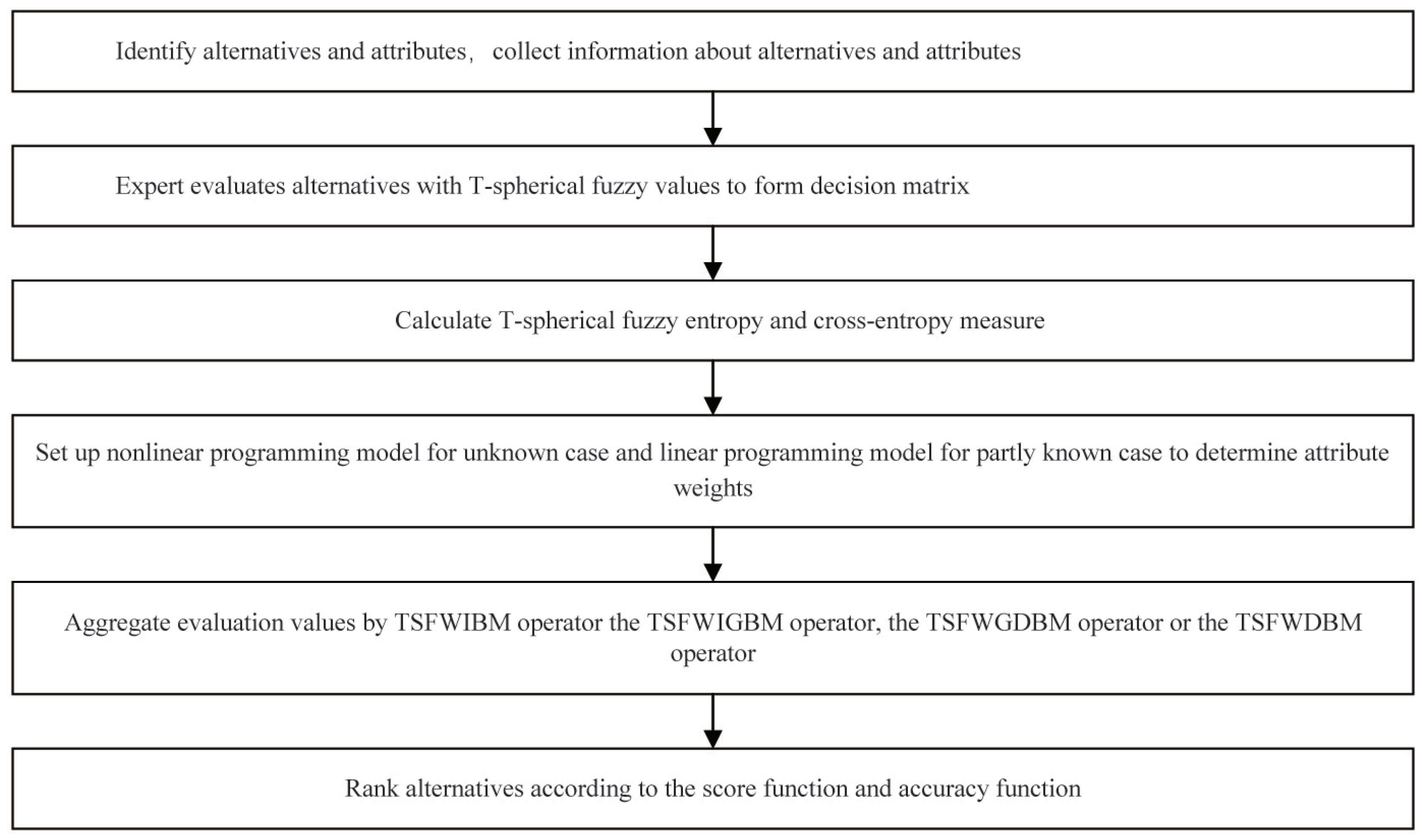
Algorithm 1 T-spherical fuzzy decision making method based on Bonferroni mean operator

Step 1. T-spherical fuzzy evaluation values ${\alpha }_{ij}(i=1,2,\cdots ,m,j=1,2,\cdots ,n)$ are given by decision makers to form T-spherical fuzzy decision matrix $D={({\alpha }_{ij})}_{m\times n}$. Step 2. Calculate the weights of attributes $w_j(j=1,2,\cdots ,n)$ using Equation (20) for completely unknown situations. $$w_j=\frac{{\sum }_{i=1}^m(\frac{1}{m-1}{\sum }_{k=1}^{m}STCE({\alpha }_{ij},{\alpha }_{kj})+(1-E({\alpha }_{ij})))}{{\sum }_{i=1}^m{\sum }_{j=1}^n(\frac{1}{m-1}{\sum }_{k=1}^{m}STCE({\alpha }_{ij},{\alpha }_{kj})+(1-E({\alpha }_{ij})))}.$$ For partly known attribute situation, Model (M-2) is used to calculate the attribute weights. Step 3. Aggregate the T-spherical fuzzy evaluation values into collective ones using the TSFWIBM operator, the TSFWIGBM operator, the TSFWGDBM operator or the TSFWDBM operator as follows $$\begin{array}{ccc}\hfill {\alpha }_i& =& {\mathrm{TSFWIBM}}_{k,l}({\alpha }_{i1},{\alpha }_{i2},\cdots ,{\alpha }_{in})\hfill \\ & =& {\left(\frac{1}{n(n-1)}{\oplus }_{s,t=1,s\ne t}^n({(w_s{\alpha }_{is})}^k\otimes {(w_t{\alpha }_{it})}^l)\right)}^{\frac{1}{k+l}}.\hfill \end{array}$$ (21) $$\begin{array}{ccc}\hfill {\alpha }_i& =& {\mathrm{TSFWIGBM}}_{k,l}({\alpha }_{i1},{\alpha }_{i2},\cdots ,{\alpha }_{in})\hfill \\ \hfill & =& \frac{1}{k+l}\left({\otimes }_{s,t=1,s\ne t}^n{((k{\alpha }_{is}^{w_s})\oplus (l{\alpha }_{it}^{w_t}))}^{\frac{1}{n(n-1)}}\right).\hfill \end{array}$$ (22) $$\begin{array}{ccc}\hfill {\alpha }_i& =& {\mathrm{TSFWDBM}}_{k,l}({\alpha }_1,{\alpha }_2,\cdots ,{\alpha }_n)\hfill \\ & =& {\left(\frac{1}{n(n-1)}{\widehat{\oplus }}_{s,t=1,s\ne t}^n({(w_s{\alpha }_{is})}^k\widehat{\otimes }{(w_t{\alpha }_{it})}^l)\right)}^{\frac{1}{k+l}}.\hfill \end{array}$$ (23) or $$\begin{array}{ccc}\hfill {\alpha }_i& =& {\mathrm{TSFWGDBM}}_{k,l}({\alpha }_{i1},{\alpha }_{i2},\cdots ,{\alpha }_{in})\hfill \\ & =& \frac{1}{k+l}\left({\widehat{\otimes }}_{s,t=1,s\ne t}^n{((k{\alpha }_{is}^{w_s})\widehat{\oplus }(l{\alpha }_{it}^{w_t}))}^{\frac{1}{n(n-1)}}\right).\hfill \end{array}$$ (24) Step 4. Rank ${\alpha }_i(i=1,2,\cdots ,m)$ according to Definition 4 and select the optimal alternative.

Figure 1. Flowchart of decision making method based on Bonferroni mean operator.

7. Numerical Example

Increasingly, students are entering university for higher education due to the development of Chinese higher education. Some old campuses are located in the city center, and there is no room for new buildings to accommodate more students. Some universities choose to construct new campuses in rural areas. There is a university constructing a new campus in Gaoxin district of Xi’an city. Several new dormitory buildings for students have been built, and there is the need to purchase new furniture.

The following attributes are considered: $C_1—$price, $C_2—$quality, $C_3—$after-sales service, $C_4—$transportation cost and $C_5—$convenience of use. The university rear service group invited several experts from different fields, including the purchasing department, finance department etc. There were five furniture companies left for further select after pre-evaluation: $A_1—$Zhongwei furniture company, $A_2—$Jongtay furniture company, $A_3—$Yongnuo furniture company, $A_4—$Yicai furniture company and $A_5—$Jiheng furniture company. The proposed algorithm is used to select the best furniture company. $t=3$.

Step 1. The T-spherical fuzzy evaluation values are given by experts, and a decision matrix is formed as $D={({\alpha }_{ij})}_{5\times 5}$ in Table 1.

Table 1. The decision matrix.

	${\mathit{C}}_1$	${\mathit{C}}_2$	${\mathit{C}}_3$	${\mathit{C}}_4$	${\mathit{C}}_5$
$A_1$	$<0.7,0.3,0.2>$	$<0.3,0.3,0.4>$	$<0.5,0.2,0.4>$	$<0.4,0.3,0.4>$	$<0.2,0.4,0.3>$
$A_2$	$<0.5,0.4,0.5>$	$<0.8,0.2,0.3>$	$<0.6,0.4,0.3>$	$<0.3,0.4,0.5>$	$<0.4,0.5,0.4>$
$A_3$	$<0.4,0.4,0.5>$	$<0.6,0.5,0.4>$	$<0.8,0.3,0.2>$	$<0.5,0.4,0.2>$	$<0.2,0.3,0.2>$
$A_4$	$<0.3,0.5,0.4>$	$<0.5,0.6,0.3>$	$<0.4,0.3,0.4>$	$<0.5,0.3,0.2>$	$<0.9,0.1,0.2>$
$A_5$	$<0.6,0.3,0.4>$	$<0.2,0.4,0.3>$	$<0.3,0.4,0.3>$	$<0.7,0.1,0.3>$	$<0.5,0.3,0.5>$

Step 2. Assume the attribute weights are completely unknown and can be calculated by Equation (20). First, $E({\alpha }_{ij})$ can be calculated as as in Table 2. Then, calculate the $STCE({\alpha }_{ij},{\alpha }_{kj})=TCE({\alpha }_{ij},{\alpha }_{kj})+TCE({\alpha }_{kj},{\alpha }_{ij})$. For example $TCE({\alpha }_{12},{\alpha }_{42})=tan({0.3}^3)\ast tan(|{0.3}^3-{0.5}^3|)+tan({0.3}^3)\ast tan(|{0.3}^3-{0.6}^3|)+tan({0.4}^3)\ast tan(|{0.4}^3-{0.3}^3|)=0.0102$. $TCE({\alpha }_{42},$${\alpha }_{12})=tan({0.5}^3)\ast tan(|{0.3}^3-{0.5}^3|)+tan({0.6}^3)\ast tan(|{0.3}^3-{0.6}^3|)+tan({0.3}^3)\ast tan(|{0.4}^3-{0.3}^3|)=0.0553$. $STCE({\alpha }_{12},$${\alpha }_{42})=TCE({\alpha }_{12},$${\alpha }_{42})+TCE({\alpha }_{42},$${\alpha }_{12})=0.0102+0.0553=0.0655$. Other $STCE({\alpha }_{ij},$${\alpha }_{kj})(i,j,k=1,2,\cdots ,5)$ can be calculated similarly. By using Equation (20), the weights can be calculated as $w_1=0.1661,w_2=0.2028,$$w_3=0.1956,w_4=0.1329,w_5=0.3025$.

Table 2. Entropy of ${\alpha }_{ij}$.

$\mathit{E}({\mathit{\alpha }}_{\mathbf{ij}})$	${\mathit{C}}_1$	${\mathit{C}}_2$	${\mathit{C}}_3$	${\mathit{C}}_4$	${\mathit{C}}_5$
$A_1$	0.6490	0.9090	0.8110	0.8720	0.9650
$A_2$	0.7501	0.4610	0.7571	0.8481	0.8725
$A_3$	0.8111	0.7211	0.4800	0.8671	0.9840
$A_4$	0.9094	0.8512	0.8720	0.8670	0.2630
$A_5$	0.7200	0.9650	0.9460	0.6300	0.7500

Step 3. If the TSFWIBM operator is used to aggregate evaluation values and $t=3$, $k=2,l=2$, the aggregated results can be calculated by Equation (21) to obtain ${\alpha }_1=<0.2816,0.1957,0.2127>$, ${\alpha }_2=<0.3603,0.2519,0.2571>$, ${\alpha }_3=<0.3507,0.2444,0.2160>$, ${\alpha }_4=<0.4428,0.2560,0.2048>$, ${\alpha }_5=<0.3047,0.2013,0.2489>$.

Step 4. The scores of the ${\alpha }_i$ can be calculated as $S({\alpha }_1)=0.5026$, $S({\alpha }_2)=0.4982$, $S({\alpha }_3)=0.4963$, $S({\alpha }_4)=0.4952$, $S({\alpha }_5)=0.5027$. Then, $A_i$ can be ranked according to the scores to obtain $A_4\succ A_3\succ A_2\succ A_1\succ A_5$, and the optimal alternative is $A_4$.

For other $k,l$ considered in the TSFWIBM operator, including $k=3,4$, and $l=3,4$, the aggregated results are shown in Table 3, and the ranking results are shown in Table 4. From the results, we can see that the optimal alternative is $A_4$, and the suboptimal alternative is $A_3$ in the TSFWIBM operator. There are slight differences in ranking for different $k,l$. $A_2$ is ranked third, and $A_1$ is ranked fourth in $k=2, l=2$ and $k=2, l=3$. With the increasing k and l, $A_1$ is ranked third, and $A_2$ is ranked fourth.

Table 3. Aggregated results of the TSFWIBM operator.

	$\mathit{k}=2,\mathit{l}=2$	$\mathit{k}=2,\mathit{l}=3$	$\mathit{k}=3,\mathit{l}=3$	$\mathit{k}=3,\mathit{l}=4$
${\alpha }_1$	$<0.2816,0.1957,0.2127>$	$<0.2847,0.2042,0.2627>$	$<0.2839,0.1975,0.2824>$	$<0.2868,0.2038,0.2916>$
${\alpha }_2$	$<0.3603,0.2519,0.2571>$	$<0.3657,0.2634,0.3225>$	$<0.3666,0.2563,0.3459>$	$<0.3727,0.2652,0.3585>$
${\alpha }_3$	$<0.3507,0.2444,0.2160>$	$<0.3542,0.2494,0.2552>$	$<0.3532,0.2467,0.2747>$	$<0.3568,0.2509,0.2816>$
${\alpha }_4$	$<0.4428,0.2560,0.2048>$	$<0.4674,0.2581,0.2550>$	$<0.4468,0.2580,0.2738>$	$<0.4676,0.2609,0.2918>$
${\alpha }_5$	$<0.3047,0.2013,0.2489>$	$<0.3205,0.2059,0.3208>$	$<0.3123,0.2054,0.3448>$	$<0.3259,0.2098,0.3599>$

Table 4. Ranking results of the TSFWIBM operator.

	$\mathit{S}({\mathit{\alpha }}_1)$	$\mathit{S}({\mathit{\alpha }}_2)$	$\mathit{S}({\mathit{\alpha }}_3)$	$\mathit{S}({\mathit{\alpha }}_4)$	$\mathit{S}({\mathit{\alpha }}_5)$	Ranking Results	Optimal Alternative
$k=2,l=2$	0.5026	0.5069	0.5092	0.5307	0.5024	$A_4\succ A_3\succ A_2\succ A_1\succ A_5$	$A_4$
$k=2,l=3$	0.4982	0.4986	0.5062	0.5342	0.4956	$A_4\succ A_3\succ A_2\succ A_1\succ A_5$	$A_4$
$k=3,l=3$	0.4963	0.4955	0.5042	0.5258	0.4904	$A_4\succ A_3\succ A_1\succ A_2\succ A_5$	$A_4$
$k=3,l=4$	0.4952	0.4935	0.5037	0.5298	0.4894	$A_4\succ A_3\succ A_1\succ A_2\succ A_5$	$A_4$
$k=5,l=5$	0.5027	0.5073	0.5089	0.5086	0.5023	$A_4\succ A_3\succ A_1\succ A_2\succ A_5$	$A_4$

For the TSFWIGBM operator used in the aggregation process in Step 3, the T-spherical fuzzy aggregated results are shown in Table 5, and the ranking results are shown in Table 6 In most cases, the optimal alternative is $A_4$, and the suboptimal alternative is $A_3$ except for $k=2, l=3$, in which the optimal alternative is $A_3$, and the suboptimal alternative is $A_4$. $A_2$ is ranked third, $A_5$ is ranked fourth, and $A_1$ is ranked last in all cases. The optimal alternative is different in the TSFWIBM operator and the TSFWIGBM operator due to different characteristics of the geometric Bonferroni mean and geometric Bonferroni mean operator.

Table 5. Aggregated results of the TSFWIGBM operator.

	$\mathit{k}=2,\mathit{l}=2$	$\mathit{k}=2,\mathit{l}=3$	$\mathit{k}=3,\mathit{l}=3$	$\mathit{k}=3,\mathit{l}=4$
${\alpha }_1$	$<0.2797,0.1936,0.2075>$	$<0.2796,0.2009,0.2101>$	$<0.2793,0.1940,0.2079>$	$<0.2791,0.1994,0.2099>$
${\alpha }_2$	$<0.5740,0.2684,0.2581>$	$<0.4611,0.2680,0.2521>$	$<0.3526,0.2526,0.2414>$	$<0.3543,0.2594,0.2446>$
${\alpha }_3$	$<0.5841,0.2548,0.2189>$	$<0.4759,0.2459,0.2105>$	$<0.3533,0.2336,0.2015>$	$<0.3539,0.2356,0.2027>$
${\alpha }_4$	$<0.6248,0.2932,0.2147>$	$<0.4755,0.2663,0.1937>$	$<0.4218,0.2658,0.1933>$	$<0.4347,0.2733,0.1987>$
${\alpha }_5$	$<0.5275,0.2106,0.2478>$	$<0.4170,0.2089,0.2482>$	$<0.3038,0.2020,0.2336>$	$<0.3084,0.2043,0.2386>$

Table 6. Ranking results of the TSFWIGBM operator.

	$\mathit{S}({\mathit{\alpha }}_1)$	$\mathit{S}({\mathit{\alpha }}_2)$	$\mathit{S}({\mathit{\alpha }}_3)$	$\mathit{S}({\mathit{\alpha }}_4)$	$\mathit{S}({\mathit{\alpha }}_5)$	Ranking Results	Optimal Alternative
$k=2,l=2$	0.5028	0.5763	0.5861	0.6044	0.5611	$A_4\succ A_3\succ A_2\succ A_5\succ A_1$	$A_4$
$k=2,l=3$	0.5022	0.5314	0.5418	0.5407	0.5241	$A_3\succ A_4\succ A_2\succ A_5\succ A_1$	$A_3$
$k=3,l=3$	0.5027	0.5068	0.5116	0.5245	0.5035	$A_4\succ A_3\succ A_2\succ A_5\succ A_1$	$A_4$
$k=3,l=4$	0.5023	0.5062	0.5115	0.5270	0.5036	$A_4\succ A_3\succ A_2\succ A_5\succ A_1$	$A_4$
$k=5,l=5$	0.5025	0.5060	0.5111	0.5198	0.5037	$A_4\succ A_3\succ A_2\succ A_5\succ A_1$	$A_4$

In the TSFWDBM operator and the TSFWGDBM operator, there are more parameters, including $\gamma ,k,l$, which are more flexible comparing with the TSFWIBM operator and the TSFWIGBM operator. If the TSFWDBM operator or the TSFWGDBM operator is used in the aggregation process in Step 3, we only present the scores and ranking results for space limit. We consider $\gamma =1,2,3,4,5$ and $k,l=2,3,4$, respectively. For the TSFWDBM operator, the results are shown in Table 7.

Table 7. Ranking results of the TSFWDBM operator.

		$\mathit{S}({\mathit{\alpha }}_1)$	$\mathit{S}({\mathit{\alpha }}_2)$	$\mathit{S}({\mathit{\alpha }}_3)$	$\mathit{S}({\mathit{\alpha }}_4)$	$\mathit{S}({\mathit{\alpha }}_5)$	Ranking Results	Optimal Alternative
$\gamma =1$	$k=2,l=2$	0.3565	0.2658	0.3474	0.3512	0.3493	$A_1\succ A_4\succ A_5\succ A_3\succ A_2$	$A_1$
	$k=2,l=3$	0.3360	0.2380	0.3263	0.3294	0.3298	$A_1\succ A_5\succ A_4\succ A_3\succ A_2$	$A_1$
	$k=3,l=4$	0.3491	0.2516	0.3397	0.3428	0.3417	$A_1\succ A_4\succ A_5\succ A_3\succ A_2$	$A_1$
	$k=4,l=4$	0.3565	0.2658	0.3474	0.3512	0.3493	$A_1\succ A_4\succ A_5\succ A_3\succ A_2$	$A_1$
$\gamma =2$	$k=2,l=2$	0.4320	0.3671	0.4368	0.4381	0.4253	$A_4\succ A_3\succ A_1\succ A_5\succ A_2$	$A_4$
	$k=2,l=3$	0.4135	0.3916	0.4574	0.4527	0.4402	$A_3\succ A_4\succ A_5\succ A_1\succ A_2$	$A_3$
	$k=3,l=4$	0.4424	0.4131	0.4690	0.4649	0.4542	$A_3\succ A_4\succ A_5\succ A_2\succ A_1$	$A_3$
	$k=4,l=4$	0.4399	0.4108	0.4651	0.4600	0.4522	$A_3\succ A_4\succ A_5\succ A_1\succ A_2$	$A_3$
$\gamma =3$	$k=2,l=2$	0.4691	0.4496	0.4958	0.4865	0.4850	$A_3\succ A_4\succ A_5\succ A_1\succ A_2$	$A_3$
	$k=2,l=3$	0.4618	0.4465	0.4936	0.4837	0.4831	$A_3\succ A_4\succ A_5\succ A_1\succ A_2$	$A_3$
	$k=3,l=4$	0.4737	0.4609	0.5010	0.4914	0.4860	$A_3\succ A_4\succ A_5\succ A_1\succ A_2$	$A_3$
	$k=4,l=4$	0.4703	0.4555	0.4969	0.4879	0.4819	$A_3\succ A_4\succ A_5\succ A_1\succ A_2$	$A_3$
$\gamma =4$	$k=2,l=2$	0.4833	0.4741	0.5162	0.5009	0.5048	$A_3\succ A_5\succ A_4\succ A_1\succ A_2$	$A_3$
	$k=2,l=3$	0.4795	0.4732	0.5139	0.4989	0.5039	$A_3\succ A_5\succ A_4\succ A_1\succ A_2$	$A_3$
	$k=3,l=4$	0.4867	0.4828	0.5209	0.5049	0.5052	$A_3\succ A_5\succ A_4\succ A_1\succ A_2$	$A_3$
	$k=4,l=4$	0.4842	0.4787	0.5177	0.5019	0.5028	$A_3\succ A_5\succ A_4\succ A_1\succ A_2$	$A_3$
$\gamma =5$	$k=2,l=2$	0.4925	0.4902	0.5295	0.5095	0.5179	$A_3\succ A_5\succ A_4\succ A_1\succ A_2$	$A_3$
	$k=2,l=3$	0.4931	0.4909	0.5300	0.5099	0.5184	$A_3\succ A_5\succ A_4\succ A_1\succ A_2$	$A_3$
	$k=3,l=4$	0.4928	0.4905	0.5298	0.5097	0.5181	$A_3\succ A_5\succ A_4\succ A_1\succ A_2$	$A_3$
	$k=4,l=4$	0.4925	0.4902	0.5295	0.5095	0.5179	$A_3\succ A_5\succ A_4\succ A_1\succ A_2$	$A_3$

The optimal alternative is $A_3$ in most cases. With the increasing of $\gamma ,k,l$, the ranking becomes $A_3\succ A_4\succ A_5\succ A_1\succ A_2$ and $A_3\succ A_5\succ A_4\succ A_1\succ A_2$. If $\gamma =1$ in the TSFWDBM operator, the optimal alternative is $A_1$ and the suboptimal alternative is $A_4$ or $A_5$. $A_4$ is the optimal alternative if $\gamma =2,k=2,l=2$ in the TSFWDBM operator.

For the TSFWGDBM operator, the results are shown in Table 8. $A_3,A_4,A_2$ are the top three alternatives and ranking of $A_1,A_5$ is different for different parameters. Since each operator has its own characteristics and focuses on each aspect of the problem, the different rankings are reasonable. For example, the $\gamma ,k,l$ can be seen as the risk attitude of the decision maker. Decision makers are more risk seeking with the increasing of $\gamma ,k,l$.

Table 8. Ranking results of the TSFWGDBM operator.

		$\mathit{S}({\mathit{\alpha }}_1)$	$\mathit{S}({\mathit{\alpha }}_2)$	$\mathit{S}({\mathit{\alpha }}_3)$	$\mathit{S}({\mathit{\alpha }}_4)$	$\mathit{S}({\mathit{\alpha }}_5)$	Ranking Results	Optimal Alternative
$\gamma =1$	$k=2,l=2$	0.6267	0.7062	0.7157	0.7110	0.6439	$A_3\succ A_4\succ A_2\succ A_5\succ A_1$	$A_3$
	$k=2,l=3$	0.6435	0.7233	0.7282	0.7310	0.6611	$A_3\succ A_4\succ A_2\succ A_5\succ A_1$	$A_3$
	$k=3,l=4$	0.6117	0.6903	0.7024	0.6944	0.6290	$A_3\succ A_4\succ A_2\succ A_5\succ A_1$	$A_3$
	$k=4,l=4$	0.6261	0.7062	0.7157	0.7110	0.6439	$A_3\succ A_4\succ A_2\succ A_5\succ A_1$	$A_3$
$\gamma =2$	$k=2,l=2$	0.5400	0.5788	0.5983	0.5876	0.5434	$A_3\succ A_4\succ A_2\succ A_5\succ A_1$	$A_3$
	$k=2,l=3$	0.5456	0.5862	0.6002	0.5953	0.5491	$A_3\succ A_4\succ A_2\succ A_5\succ A_1$	$A_3$
	$k=3,l=4$	0.5364	0.5760	0.5961	0.5861	0.5422	$A_3\succ A_4\succ A_2\succ A_5\succ A_1$	$A_3$
	$k=4,l=4$	0.5400	0.5788	0.5983	0.5876	0.5434	$A_3\succ A_4\succ A_2\succ A_5\succ A_1$	$A_3$
$\gamma =3$	$k=2,l=2$	0.5159	0.5360	0.5570	0.5463	0.5149	$A_3\succ A_4\succ A_2\succ A_5\succ A_1$	$A_3$
	$k=2,l=3$	0.5190	0.5408	0.5580	0.5505	0.5177	$A_3\succ A_4\succ A_2\succ A_1\succ A_5$	$A_3$
	$k=3,l=4$	0.5132	0.5317	0.5550	0.5427	0.5123	$A_3\succ A_4\succ A_2\succ A_1\succ A_5$	$A_3$
	$k=4,l=4$	0.5159	0.5360	0.5570	0.5463	0.5149	$A_3\succ A_4\succ A_2\succ A_1\succ A_5$	$A_3$
$\gamma =4$	$k=2,l=2$	0.5043	0.5145	0.5354	0.5235	0.5013	$A_3\succ A_4\succ A_2\succ A_5\succ A_1$	$A_3$
	$k=2,l=3$	0.5065	0.5180	0.5360	0.5261	0.5031	$A_3\succ A_4\succ A_2\succ A_5\succ A_1$	$A_3$
	$k=3,l=4$	0.5024	0.5114	0.5340	0.5210	0.4996	$A_3\succ A_4\succ A_2\succ A_5\succ A_1$	$A_3$
	$k=4,l=4$	0.5043	0.5145	0.5354	0.5235	0.5013	$A_3\succ A_4\succ A_2\succ A_5\succ A_1$	$A_3$
$\gamma =5$	$k=2,l=2$	0.4973	0.5012	0.5221	0.5085	0.4928	$A_3\succ A_4\succ A_2\succ A_5\succ A_1$	$A_3$
	$k=2,l=3$	0.4990	0.5040	0.5226	0.5104	0.4941	$A_3\succ A_4\succ A_2\succ A_1\succ A_5$	$A_3$
	$k=3,l=4$	0.4958	0.4988	0.5210	0.5066	0.4915	$A_3\succ A_4\succ A_2\succ A_1\succ A_5$	$A_3$
	$k=4,l=4$	0.4973	0.5012	0.5221	0.5085	0.4928	$A_3\succ A_4\succ A_2\succ A_1\succ A_5$	$A_3$

8. Advantages and Comparison Analysis

Advantages

The T-SFS can be reduced to some other fuzzy sets, including the spherical fuzzy set, Pythagorean fuzzy set, q-rung orthopair fuzzy set, picture fuzzy set, intuitionistic fuzzy set etc. Then, the proposed operators can be reduced to some other fuzzy aggregation operators.

1. If all the values satisfy $0\le {\mu }_{\tilde{A}}^t+{\eta }_{\tilde{A}}^t+{\nu }_{\tilde{A}}^t\le 1,t=2$, then the TSFIBM operator becomes the spherical fuzzy interaction Bonferroni mean (SFIBM) operator, the TSFIGBM operator becomes the spherical fuzzy interaction geometric Bonferroni mean (SFIGBM) operator. Other T-spherical fuzzy Bonferroni mean operators also reduce to the corresponding spherical fuzzy Bonferroni mean operators.

2. If all the values satisfy $0\le {\mu }_{\tilde{A}}^t+{\eta }_{\tilde{A}}^t+{\nu }_{\tilde{A}}^t\le 1,t=1$, then the TSFIBM operator becomes the picture fuzzy interaction Bonferroni mean (PFIBM) operator, and the TSFIGBM operator becomes the picture fuzzy interaction geometric Bonferroni mean (PFIGBM) operator. Other T-spherical fuzzy Bonferroni mean operators also reduce to the corresponding picture fuzzy Bonferroni mean operators.

3. If all the values satisfy $0\le {\mu }_{\tilde{A}}^t+{\eta }_{\tilde{A}}^t+{\nu }_{\tilde{A}}^t\le 1,$ and ${\eta }_{\tilde{A}}=0$, then the TSFIBM operator becomes the q-rung orthopair fuzzy interaction Bonferroni mean (q-ROFIBM) operator, the TSFIGBM operator becomes the q-rung orthopair fuzzy interaction geometric Bonferroni mean (q-ROFIGBM) operator. Other T-spherical fuzzy Bonferroni mean operators also reduce to the corresponding q-rung orthopair fuzzy Bonferroni mean operators.

4. If all the values satisfy $0\le {\mu }_{\tilde{A}}^t+{\eta }_{\tilde{A}}^t+{\nu }_{\tilde{A}}^t\le 1,t=2$ and ${\eta }_{\tilde{A}}=0$, then the TSFIBM operator becomes the Pythagorean fuzzy interaction Bonferroni mean (PyFIBM) operator, the TSFIGBM operator becomes the Pythagorean fuzzy interaction geometric Bonferroni mean (PyFIGBM) operator. Other T-spherical fuzzy Bonferroni mean operators also reduce to the corresponding Pythagorean fuzzy Bonferroni mean operators.

5. If all the values satisfy $0\le {\mu }_{\tilde{A}}^t+{\eta }_{\tilde{A}}^t+{\nu }_{\tilde{A}}^t\le 1,t=1$ and ${\eta }_{\tilde{A}}=0$, then the TSFIBM operator becomes the intuitionistic fuzzy interaction Bonferroni mean (IFIBM) operator, and the TSFIGBM operator becomes the intuitionistic fuzzy interaction geometric Bonferroni mean (IFIGBM) operator. Other T-spherical fuzzy Bonferroni mean operators also reduce to the corresponding intuitionistic fuzzy Bonferroni mean operators.

Here, an example from He and He [74] is taken to illustrate the advantages of the proposed algorithm. Consider the alternative set $\{A_1,A_2,A_3,A_4,A_5\}$ and attribute set $\{C_1,C_2,C_3\}$. The decision matrix is shown in Table 9. The data can be expressed as T-spherical fuzzy values shown in Table 10. Since all the values in Table 10 can satisfy $0\le {\mu }_{\tilde{A}}^t+{\eta }_{\tilde{A}}^t+{\nu }_{\tilde{A}}^t\le 1,t=1$, we take $t=1$. The weight vector is taken as $(0.30,0.50,0.20)$ and $p=q=1$, which is the same as that in reference [74].

Table 9. Intuitionistic decision matrix.

	${\mathit{C}}_1$	${\mathit{C}}_2$	${\mathit{C}}_3$
$A_1$	$<0.3,0.4>$	$<0.7,0.2>$	$<0.5,0.3>$
$A_2$	$<0.5,0.2>$	$<0.4,0.1>$	$<0.7,0.1>$
$A_3$	$<0.4,0.5>$	$<0.7,0.2>$	$<0.4,0.4>$
$A_4$	$<0.2,0.6>$	$<0.8,0.1>$	$<0.8,0.2>$
$A_5$	$<0.9,0.1>$	$<0.6,0.3>$	$<0.2,0.5>$

Table 10. T-spherical fuzzy decision matrix.

	${\mathit{C}}_1$	${\mathit{C}}_2$	${\mathit{C}}_3$
$A_1$	$<0.3,0,0.4>$	$<0.7,0,0.2>$	$<0.5,0,0.3>$
$A_2$	$<0.5,0,0.2>$	$<0.4,0,0.1>$	$<0.7,0,0.1>$
$A_3$	$<0.4,0,0.5>$	$<0.7,0,0.2>$	$<0.4,0,0.4>$
$A_4$	$<0.2,0,0.6>$	$<0.8,0,0.1>$	$<0.7,0,0.2>$
$A_5$	$<0.8,0,0.1>$	$<0.6,0,0.3>$	$<0.2,0,0.5>$

Then, the aggregated values using the TSFIWBM${}_{1,1}$ operator are as ${\alpha }_1={\mathrm{TSFIWBM}}_{1,1}$$({\alpha }_{11},$${\alpha }_{12},{\alpha }_{13})=<0.2546,0,0.2028>,$${\alpha }_2=<0.1956,0,0.0816>$, ${\alpha }_3=<0.2198,0,0.2606>$, ${\alpha }_4=<0.2636,0,0.2009>$, ${\alpha }_5=<0.26110,0.2093>$. The scores can be calculated as $S({\alpha }_1)=0.05176,$$S({\alpha }_2)=0.1140,$$S({\alpha }_3)=-0.0408,$$S({\alpha }_2)=0.0627,$$S({\alpha }_2)=0.05183.$ Then, the alternatives can be ranked as $A_2\succ A_4\succ A_5\succ A_1\succ A_3.$ The proposed results are the same as that in [74]. Hence, the proposed algorithm is the generalization of the existing work and it can solve the problems more broadly than the existing one. Other fuzzy structures can be used similarly if the conditions are satisfied.

Comparison analysis

In order to further illustrate the proposed method, we compare it with some other decision making methods, including the method base on the T-spherical fuzzy weighted aggregation operators, T-spherical fuzzy TOPSIS, T-spherical fuzzy VIKOR method and T-spherical fuzzy TODIM method. The attribute weight vector is also taken as $(0.1661,0.2028,$$0.1956,$$0.1329,$$0.3025)$, which is the same as in the above section. The decision matrix is also the same as that in Table 1.

If T-spherical fuzzy weighted aggregation operators are used, aggregation results are shown in Table 11 and ranking results are shown in Table 12. If the TSFWA operator is used in the aggregation step, the ranking result is $A_4\succ A_3\succ A_2\succ A_5\succ A_1$. If the TSFWGA operator is used, the ranking result is $A_4\succ A_2\succ A_3\succ A_1\succ A_5$. The optimal alternative is the same for these two operators, but the ranking is different for other alternatives. If the TSFIWA operator or the TSFIGWA operator is used in Step 3, the ranking is $A_4\succ A_3\succ A_2\succ A_5\succ A_1$. In the TSFIWA operator or the TSFIGWA operator, the interaction operations are considered.

Table 11. Aggregated results of different operators.

	TSFWA	TSFWGA	TSFIWA	TSFIGWA
${\alpha }_1$	$<0.4741,0.3023,0.3268>$	$<0.3507,0.3262,0.3524>$	$<0.4741,0.3233,0.3473>$	$<0.4703,0.3253,0.3524>$
${\alpha }_2$	$<0.5968,0.3718,0.3813>$	$<0.4978,0.4161,0.4089>$	$<0.5968,0.4004,0.3985>$	$<0.5839,0.4171,0.4089>$
${\alpha }_3$	$<0.5830,0.3626,0.2680>$	$<0.4154,0.3886,0.3416>$	$<0.5830,0.3895,0.3386>$	$<0.5813,0.3910,0.3419>$
${\alpha }_4$	$<0.7160,0.2696,0.2790>$	$<0.5253,0.4266,0.3189>$	$<0.7160,0.3809,0.2965>$	$<0.6963,0.4279,0.3189>$
${\alpha }_5$	$<0.5115,0.2907,0.3673>$	$<0.4050,0.3378,0.3996>$	$<0.5115,0.3299,0.4003>$	$<0.5090,0.3366,0.3996>$

Table 12. Ranking results of different operators.

	$\mathit{S}({\mathit{\alpha }}_1)$	$\mathit{S}({\mathit{\alpha }}_2)$	$\mathit{S}({\mathit{\alpha }}_3)$	$\mathit{S}({\mathit{\alpha }}_4)$	$\mathit{S}({\mathit{\alpha }}_5)$	Ranking Results	Optimal Alternative
TSFWA	0.5220	0.5539	0.5656	0.6629	0.5298	$A_4\succ A_3\succ A_2\succ A_5\succ A_1$	$A_4$
TSFWGA	0.4823	0.4915	0.4866	0.5174	0.4820	$A_4\succ A_2\succ A_3\succ A_1\succ A_5$	$A_4$
TSFIWA	0.5154	0.5425	0.5501	0.6429	0.5169	$A_4\succ A_3\succ A_2\succ A_5\succ A_1$	$A_4$
TSFIGWA	0.5129	0.5291	0.5484	0.6134	0.5150	$A_4\succ A_3\succ A_2\succ A_5\succ A_1$	$A_4$

If the T-spherical fuzzy TOPSIS method is used to solve the problem, the first two steps are the same. The T-spherical fuzzy weighted decision matrix is calculated as $D^{\prime }=({\alpha }_{ij}^{\prime })=(w_j{\alpha }_{ij})$. The T-spherical fuzzy positive ideal solution ${\alpha }^{+}=({\alpha }_1^{+},{\alpha }_2^{+},\cdots ,{\alpha }_5^{+})=(max{\alpha }_{i1},max{\alpha }_{i2},\cdots ,max{\alpha }_{i5})=(<0.4069,0.1864,0.1252>,<0.5135,0.1425,0.2159>,<0.5078,0.2127,0.1432>,<0.3787,$$0.0576,0.1740>,<0.6885,0.0910,0.1827>)$. The T-spherical fuzzy negative ideal solution ${\alpha }^{-}=({\alpha }_1^{-},{\alpha }_2^{-},\cdots ,{\alpha }_5^{-})=(min{\alpha }_{i1},min{\alpha }_{i2},\cdots ,$$min{\alpha }_{i5})$$=(<0.1655,0.2822,0.2327>,<0.2990,0.3789,0.1980>,<0.1748,0.2360,0.1794>,<0.1537,$$0.2078,0.2679>,<0.2706,$$0.3465,0.2846>)$. The collective distances of each alternative to the ${\alpha }^{+}$ and ${\alpha }^{-}$ are defined as

$$d_i^{+}=\frac{1}{5}\sum _{j=1}^{5}d({\alpha }_{ij},{\alpha }_j^{+})=\frac{1}{5}\sum _{j=1}^5(|{({\mu }_{{\alpha }_{ij}})}^3-{({\mu }_{{\alpha }_{ij}}^{+})}^3|+|{({\eta }_{{\alpha }_{ij}})}^3-{({\eta }_{{\alpha }_{ij}}^{+})}^3|+|{({\nu }_{{\alpha }_{ij}})}^3-{({\nu }_{{\alpha }_{ij}}^{+})}^3|),$$

$$d_i^{-}=\frac{1}{5}\sum _{j=1}^{5}d({\alpha }_{ij},{\alpha }_j^{-})=\frac{1}{5}\sum _{j=1}^5(|{({\mu }_{{\alpha }_{ij}})}^3-{({\mu }_{{\alpha }_{ij}}^{-})}^3|+|{({\eta }_{{\alpha }_{ij}})}^3-{({\eta }_{{\alpha }_{ij}}^{-})}^3|+|{({\nu }_{{\alpha }_{ij}})}^3-{({\nu }_{{\alpha }_{ij}}^{-})}^3|).$$

$d_i^{+}$ and $d_i^{-}$ can be calculated as $d_1^{+}=0.3738$, $d_2^{+}=0.3645$, $d_3^{+}=0.3646$, $d_4^{+}=0.3213$, $d_5^{+}=0.3494$, $d_1^{-}=0.3121$, $d_2^{-}=0.1823$, $d_3^{-}=0.2914$, $d_4^{-}=0.2538$, $d_5^{-}=0.2752$. Calculate the T-spherical fuzzy closeness coefficients by $C_i=\frac{d_i^{-}}{d_i^{-}+d_i^{+}}$ to obtain $C_1=0.4550$, $C_2=0.3334$, $C_3=0.4442$, $C_4=0.4413$, $C_5=0.4406$. The alternatives can be ranked as $A_1\succ A_3\succ A_4\succ A_5\succ A_2$ and the optimal alternative is $A_1$.

If the T-spherical fuzzy VIKOR method is used, the first two steps are also the same. The utility index $S_i$ is calculated by the following equation

$$S_i=w_1\frac{d({\alpha }_{i1},{\alpha }_1^{+})}{d({\alpha }_1^{+},{\alpha }_1^{-})}+w_2\frac{d({\alpha }_{i2},{\alpha }_2^{+})}{d({\alpha }_2^{+},{\alpha }_2^{-})}+\cdots +w_5\frac{d({\alpha }_{i5},{\alpha }_5^{+})}{d({\alpha }_5^{+},{\alpha }_5^{-})}.$$

$S_1=0.7617$, $S_2=0.6718$, $S_3=0.6553$, $S_4=0.6104$, $S_5=0.7373$. We rank alternatives according to $S_i$ to obtain $A_4\succ A_3\succ A_2\succ A_5\succ A_1$. The regret index is calculated by the following equation

$$R_i=max\{w_1\frac{d({\alpha }_{i1},{\alpha }_1^{+})}{d({\alpha }_1^{+},{\alpha }_1^{-})},w_2\frac{d({\alpha }_{i2},{\alpha }_2^{+})}{d({\alpha }_2^{+},{\alpha }_2^{-})},\cdots ,w_5\frac{d({\alpha }_{i5},{\alpha }_5^{+})}{d({\alpha }_5^{+},{\alpha }_5^{-})}\}.$$

$R_1=0.3025$, $R_2=0.3025$, $R_3=0.2475$, $R_4=0.2028$, $R_5=0.2475$. Rank alternatives according to $R_i$ to obtain $A_4\succ A_3\sim A_5\succ A_1\sim A_2$. The collective index can be calculated by

$$Q_i=v\frac{S_i-S^{+}}{S^{-}-S^{+}}+(1-v)\frac{R_i-R^{+}}{R^{-}-R^{+}},$$

where $S^{+}=min{S}_i$, $S^{-}=max{S}_i$, $R^{+}=min{R}_i$, $R^{-}=max{R}_i$. If $v=0.5$, $Q_1=1$, $Q_2=0.7029$, $Q_3=0.3726$, $Q_4=0$, $Q_5=0.6435$. The alternatives can be ranked as $A_4\succ A_3\succ A_5\succ A_2\succ A_1$. If other $v=0,0.2,0.4,0.6,0.8,1.0$ are used, $Q_i$ can be calculated and results are shown in Table 13. The optimal alternative is always $A_4$ and suboptimal alternative is $A_3$. There are slightly differences in the ranking of $A_5$ and $A_2$ for different v.

Table 13. $Q_i$ values of different v and compromise solutions.

	v	${\mathit{A}}_1$	${\mathit{A}}_2$	${\mathit{A}}_3$	${\mathit{A}}_4$	${\mathit{A}}_5$	Ranking Results	Compromise Solutions
$Q(v)$	0	1.0	1.0	0.4484	0.0	0.4484	$A_4\succ A_3\sim A_5\succ A_2\sim A_1$	$A_4$
$Q(v)$	0.2	1.0	0.8812	0.4181	0.0	0.5264	$A_4\succ A_3\succ A_5\succ A_2\succ A_1$	$A_4$
$Q(v)$	0.4	1.0	0.7633	0.3877	0.0	0.6045	$A_4\succ A_3\succ A_5\succ A_2\succ A_1$	$A_4$
$Q(v)$	0.6	1.0	0.6435	0.3574	0.0	0.6825	$A_4\succ A_3\succ A_2\succ A_5\succ A_1$	$A_4$
$Q(v)$	0.8	1.0	0.5247	0.3271	0.0	0.7606	$A_4\succ A_3\succ A_2\succ A_5\succ A_1$	$A_4$
$Q(v)$	1.0	1.0	0.4058	0.2968	0.0	0.8386	$A_4\succ A_3\succ A_2\succ A_5\succ A_1$	$A_4$

If the T-spherical fuzzy TODIM method is used in decision making, the first two steps are the same as other methods. The relative weights are calculated as $w_{jk}=\frac{w_j}{w_k}$, $w_k={max}_j\left\{w_j\right\}$. $w_{1k}=0.5490,$ $w_{2k}=0.6704,$$w_{3k}=0.6466,$$w_{4k}=0.4393,$$w_{5k}=1.0.$ The dominant degree of $A_i$ over $A_j$ with regard to $C_k$ is defined as

$${\varphi }_k(A_i,A_j)=\left\{\begin{array}{c}\sqrt{\frac{w_{jk}}{{\sum }_{j=1}^n{w}_{jk}}d({\alpha }_{ik},{\alpha }_{jk})},\mathrm{if}S({\alpha }_{ik})>S({\alpha }_{jk})\hfill \\ 0,\mathrm{if}S({\alpha }_{ik})=S({\alpha }_{jk})\hfill \\ -\frac{1}{\tau }\sqrt{\frac{{\sum }_{j=1}^n{w}_{jk}}{w_{jk}}d({\alpha }_{ik},{\alpha }_{jk})},\mathrm{if}S({\alpha }_{ik})<S({\alpha }_{jk})\hfill \end{array}\right.$$

(25)

Here, $\tau =1$. Then, ${\varphi }_k(A_i,A_j)={\sum }_{k=1}^5{\varphi }_k(A_i,A_j)$. The results are shown in Table 14. The prospect value $\psi (A_i(i=1,2,\cdots ,5))$ can be calculated by

$$\psi (A_i)=\frac{{\sum }_{j=1}^5\varphi (A_i,A_j)-{min}_{1\le i\le 5}\{{\sum }_{j=1}^5\varphi (A_i,A_j)\}}{{max}_{1\le i\le 5}\{{\sum }_{j=1}^5\varphi (A_i,A_j)\}-{min}_{1\le i\le 5}\{{\sum }_{j=1}^5\varphi (A_k,A_j)\}}.$$

(26)

Then, $\psi (A_1)=0.5065$, $\psi (A_2)=0.8018$, $\psi (A_3)=0$, $\psi (A_4)=1.0$, $\psi (A_5)=0.1966$. The alternatives can be ranked as $A_4\succ A_2\succ A_1\succ A_5\succ A_3$.

Table 14. Global dominance of $A_i$ over $A_j$.

	${\mathit{A}}_1$	${\mathit{A}}_2$	${\mathit{A}}_3$	${\mathit{A}}_4$	${\mathit{A}}_5$
$A_1$	0.0	−3.8964	−0.9154	−4.1311	−3.4218
$A_2$	−2.4244	0.0	−1.5323	−3.9547	−2.2853
$A_3$	−5.5283	−4.3000	0.0	−3.6430	−2.6115
$A_4$	−2.4980	−3.1172	−1.7797	0.0	−1.3468
$A_5$	−2.7504	−4.4510	−2.9578	−4.4807	0.0

Comparison summary

The main difference between the existing methods and the proposed methods are summarized in Table 15. The evaluation values are given as TSF values, which are more flexible and powerful. The interrelation between T-spherical fuzzy input arguments are considered using the Bonferroni mean. The interaction operations between the membership degree, the abstinence degree and the non-membership degree are considered.

Table 15. Comparison of TSF aggregation method with other methods.

Methods	Information by TFS Fuzzy Values	Whether the Interrelationships Are Considered between Arguments	Whether a Parameter Existing to Manipulate the Results
TSFWA [7]	Yes	No	No
TSFWGA	Yes	No	No
TSFIWA [14]	Yes	No	No
TSFIWGA [14]	Yes	No	No
TSF-TOPSIS [9]	Yes	No	No
TSF-VIKOR	Yes	No	No
TSF-TODIM [14]	Yes	No	No
Karaaslan and Dawood [34]	Yes	No	Yes
Park et al. [44]	No	No	No
Wei et al. [45]	No	Yes	No
TSFWIBM	Yes	Yes	No
TSFWIGBM	Yes	Yes	No
TSFWDBM	Yes	Yes	Yes
TSFWGDBM	Yes	Yes	Yes

The Dombi and Bonferroni mean are used at the same time in T-spherical fuzzy environments to make aggregation more flexible. Existing T-spherical fuzzy methods do not have all these characteristics.

9. Conclusions

In this paper, some T-spherical fuzzy Bonferroni mean aggregation operators were developed. The main findings are as follows. By considering interaction laws, T-spherical fuzzy Bonferroni mean aggregation operators were developed, including the TSFIBM operator, the TSFIGBM operator, the TSFIWBM operatror and the TSFIWGBM operator. The properties of the operators were studied, including the idempotency and boundedness.

Then, T-spherical fuzzy Dombi Bonferroni mean aggregation operators were developed using the Dombi mean and Bonferroni mean, including the TSFDBM operator, the TSFGDBM operator, the TSFWDBM operator and the TSFWGDBM operator. New T-spherical fuzzy entropy and cross-entropy measures were defined, and an attribute weight determining method based on these was developed. The new T-spherical fuzzy multiple attribute decision making method based on the T-spherical fuzzy Bonferroni mean operators were defined, and the dormitory furniture procurement problem was presented to illustrate the algorithm.

The weakness of the method is that it cannot deal with problems with multiple types of decision information. In the future, we will study some useful tools to model uncertain information and related concepts, including the properties, set-theoretic operations and axiomatic results of the refined Pythagorean Fuzzy Sets. We will study further T-spherical fuzzy decision making methods to deal with decision problems with special characteristics. We will also apply newly developed algorithms to deal with more real complicated decision problems.

References

1. Ashraf, S.; Abdullah, S.; Aslam, M.; Qiyas, M.; Kutbi, M.A. Spherical fuzzy sets and its representation of spherical fuzzy t-norms and t-conorms. J. Intell. Fuzzy Syst. 2019, 36, 6089–6102. [Google Scholar] [CrossRef]
2. Atanassov, K.T. Intuitionistic fuzzy sets. Fuzzy Sets Syst. 1986, 20, 87–96. [Google Scholar] [CrossRef]
3. Paul, A.E.; Johnson, M.A. Similarity-Distance Decision-Making Technique and its Applications via Intuitionistic Fuzzy Pairs. J. Comput. Cogn. Eng. 2022; in press. [Google Scholar]
4. Mehmet, Ü.; Murat, O.; Ezgi, T. Cosine and Cotangent Similarity Measures Based on Choquet Integral for Spherical Fuzzy Sets and Applications to Pattern Recognition. J. Comput. Cogn. Eng. 2022, 1, 1–11. [Google Scholar]
5. Khan, M.R.; Ullah, K.; Pamucar, D.; Bari, M. Performance Measure Using a Multi-Attribute Decision Making Approach Based on Complex T-Spherical Fuzzy Power Aggregation Operators. J. Comput. Cogn. Eng. 2022; in press. [Google Scholar]
6. Ashraf, S.; Abdullah, S. Spherical aggregation operators and their application in multiattribute group decision-making. Int. J. Intell. Syst. 2019, 34, 493–523. [Google Scholar] [CrossRef]
7. Donyatalab, Y.; Farokhizadeh, E.; Garmroodi, S.D.S.; Shishavan, S.A.S. Harmonic mean aggregation operators in spherical fuzzy environment and their group decision making applications. J. Mult.-Valued Log. Soft Comput. 2019, 33, 565–592. [Google Scholar]
8. Mahmood, T.; Ullah, K.; Khan, Q.; Jan, N. An approach toward decision-making and medical diagnosis problems using the concept of spherical fuzzy sets. Int. J. Intell. Syst. 2019, 31, 7041–7053. [Google Scholar] [CrossRef]
9. Zeng, S.Z.; Munir, M.; Mahmood, T.; Naeem, M. Some T-spherical fuzzy Einstein interactive aggregation operators and their application to selection of photovoltaic cells. Math. Probl. Eng. 2020, 2020, 1904362. [Google Scholar] [CrossRef]
10. Zeng, S.Z.; Garg, H.; Munir, M.; Mahmood, T.; Hussain, A. A multi-attribute decision making process with immediate probabilistic interactive averaging aggregation operators of T-spherical fuzzy sets and its application in the selection of solar cells. Energies 2019, 12, 4436. [Google Scholar] [CrossRef] [Green Version]
11. Al-Quran, A. A new multi attribute decision making method based on the T-Spherical hesitant fuzzy sets. IEEE Access 2021, 9, 156200–156210. [Google Scholar] [CrossRef]
12. Jan, N.; Mahmood, T.; Zedam, L.; Abdullah, L.; Ullah, K. Analysis of double domination using the concept of spherical fuzzy information with application. J. Ambient. Intell. Humaniz. Comput. 2022; in press. [Google Scholar] [CrossRef]
13. Munir, M.; Kalsoom, H.; Ullah, K.; Mahmood, T.; Chu, Y.M. T-spherical fuzzy Einstein hybrid aggregation operators and their applications in multi-attribute decision making problems. Symmetry 2020, 12, 365. [Google Scholar] [CrossRef] [Green Version]
14. Ju, Y.B.; Liang, Y.Y.; Luo, C.; Dong, P.W.; Gonzalez, E.D.R.S.; Wang, A.H. T-spherical fuzzy TODIM method for multi-criteria group decision-making problem with incomplete weight information. Soft Comput. 2021, 25, 2981–3001. [Google Scholar] [CrossRef]
15. Xian, S.D.; Cheng, Y.; Chen, K.Y. A novel weighted spatial T-spherical fuzzy C-means algorithms with bias correction for image segmentation. Int. J. Intell. Syst. 2022, 37, 1239–1272. [Google Scholar] [CrossRef]
16. Zedam, L.; Jan, N.; Rak, E.; Mahmood, T.; Ullah, K. An approach towards decision-making and shortest path problems based on T-spherical fuzzy information. Int. J. Fuzzy Syst. 2020, 22, 1521–1534. [Google Scholar] [CrossRef]
17. Guleria, A.; Bajaj, R.K. T-spherical fuzzy graphs: Operations and applications in various selection processes. Arab. J. Sci. Eng. 2020, 45, 2177–2193. [Google Scholar] [CrossRef]
18. Mahmood, T.; Warraich, M.S.; Ali, Z.; Pamucar, D. Generalized MULTIMOORA method and Dombi prioritized weighted aggregation operators based on T-spherical fuzzy sets and their applications. Int. J. Intell. Syst. 2021, 36, 4659–4692. [Google Scholar] [CrossRef]
19. Munir, M.; Mahmood, T.; Hussain, A. Algorithm for T-spherical fuzzy MADM based on associated immediate probability interactive geometric aggregation operators. Artif. Intell. Rev. 2021, 54, 6033–6061. [Google Scholar] [CrossRef]
20. Liu, P.D.; Zhu, B.Y.; Wang, P. A multi-attribute decision-making approach based on spherical fuzzy sets for Yunnan Baiyao’s R&D project selection problem. Int. J. Fuzzy Syst. 2019, 21, 2168–2191. [Google Scholar]
21. Wang, J.C.; Chen, T.Y. A T-spherical fuzzy ELECTRE approach for multiple criteria assessment problem from a comparative perspective of score functions. J. Intell. Fuzzy Syst. 2021, 41, 3751–3770. [Google Scholar] [CrossRef]
22. Ullah, K.; Garg, H.; Mahmood, T.; Jan, N.; Ali, Z. Correlation coefficients for T-spherical fuzzy sets and their applications in clustering and multi-attribute decision making. Soft Comput. 2020, 24, 1647–1659. [Google Scholar] [CrossRef]
23. Ullah, K.; Mahmood, T.; Jan, N. Similarity measures for T-spherical fuzzy sets with applications in pattern recognition. Symmetry 2018, 10, 193. [Google Scholar] [CrossRef] [Green Version]
24. Khan, Q.; Gwak, J.; Shahzad, M.; Alam, M.K. A novel approached based on T-spherical fuzzy Schweizer-Sklar power Heronian mean operator for evaluating water reuse applications under uncertainty. Sustainability 2021, 13, 7108. [Google Scholar] [CrossRef]
25. Garg, H.; Munir, M.; Ullah, K.; Mahmood, T.; Jan, N. Algorithm for T-spherical fuzzy multi-attribute decision making based on improved interactive aggregation operators. Symmetry 2018, 10, 670. [Google Scholar] [CrossRef] [Green Version]
26. Mahmood, T.; Ahmmad, J.; Ali, Z.; Pamucar, D.; Marinkovic, D. Interval valued T-spherical fuzzy soft average aggregation operators and their applications in multiple-criteria decision making. Symmetry 2021, 13, 829. [Google Scholar] [CrossRef]
27. Garg, H.; Ullah, K.; Mahmood, T.; Hassan, N.; Jan, N. T-spherical fuzzy power aggregation operators and their applications in multi-attribute decision making. J. Ambient. Intell. Humaniz. Comput. 2021, 12, 9067–9080. [Google Scholar] [CrossRef]
28. Ullah, K.; Mahmood, T.; Garg, H. Evaluation of the performance of search and rescue robots using T-spherical fuzzy Hamacher aggregation operators. Int. J. Fuzzy Syst. 2020, 22, 570–582. [Google Scholar] [CrossRef]
29. Liu, P.D.; Ali, Z.; Mahmood, T. Novel complex T-spherical fuzzy 2-Tuple linguistic muirhead mean aggregation operators and their application to multi-aAttribute decision-making. Int. J. Intell. Syst. 2021, 14, 295–331. [Google Scholar] [CrossRef]
30. Liu, P.D.; Wang, D.Y. An extended taxonomy method based on normal T-Spherical fuzzy numbers for multiple-attribute decision-making. Int. J. Fuzzy Syst. 2022, 24, 73–90. [Google Scholar] [CrossRef]
31. Ozlu, S.; Karaaslan, F. Correlation coefficient of T-spherical type-2 hesitant fuzzy sets and their applications in clustering analysis. J. Ambient. Intell. Humaniz. Comput. 2022, 13, 329–357. [Google Scholar] [CrossRef]
32. Chen, Y.J.; Munir, M.; Mahmood, T.; Hussain, A.; Zeng, S.Z. Some generalized T-spherical and group-generalized fuzzy geometric aggregation operators with application in MADM problems. J. Math. 2021, 2021, 5578797. [Google Scholar] [CrossRef]
33. Ali, Z.; Mahmood, T.; Yang, M.S. Complex T-Spherical fuzzy aggregation operators with application to multi-attribute decision making. Symmetry 2020, 12, 1311. [Google Scholar] [CrossRef]
34. Karaaslan, F.; Dawood, M.A.D. Complex T-spherical fuzzy Dombi aggregation operators and their applications in multiple-criteria decision-making. Complex Intell. Syst. 2021, 7, 2711–2734. [Google Scholar] [CrossRef]
35. Akram, M.; Khan, A.; Karaaslan, F. Complex spherical Dombi fuzzy aggregation operators for decision-making. J. Mult.-Valued Log. Soft Comput. 2021, 37, 503–531. [Google Scholar]
36. Ibrahim, H.Z.; Al-Shami, T.M.; Elbarbary, O.G. (3,2)-Fuzzy Sets and Their Applications to Topology and Optimal Choices. Comput. Intell. Neurosci. 2021, 2021, 1272266. [Google Scholar] [CrossRef]
37. Bonferroni, C. Sulle medie multiple dipotenze. Boll. dell’unione Mat. Ital. 1950, 5, 267–270. [Google Scholar]
38. Yager, R.R. On generalized Bonferroni mean operators for multi-criteria aggregation. Int. J. Approx. Reason. 2009, 50, 1279–1286. [Google Scholar] [CrossRef] [Green Version]
39. Xia, M.M.; Xu, Z.S.; Zhu, B. Geometric Bonferroni means with their application in multi-criteria decision making. Knowl.-Based Syst. 2013, 40, 88–100. [Google Scholar] [CrossRef]
40. Li, D.Q.; Zeng, W.Y.; Li, J.H. Geometric Bonferroni mean operators. Int. J. Intell. Syst. 2016, 31, 1181–1197. [Google Scholar] [CrossRef]
41. Zhu, B.; Xu, Z.S. Hesitant fuzzy Bonferroni means for multi-criteria decision making. J. Oper. Res. Soc. 2013, 64, 1831–1840. [Google Scholar] [CrossRef]
42. Zhu, B.; Xu, Z.S.; Xia, M.M. Hesitant fuzzy geometric Bonferroni means. Inform. Sci. 2012, 205, 72–85. [Google Scholar] [CrossRef]
43. He, Y.D.; He, Z.; Jin, C.; Chen, H.Y. Intuitionistic fuzzy power geometric Bonferroni means and their application to multiple attribute group decision making. Int. J. Uncertain. Fuzziness Knowl.-Based Syst. 2015, 23, 285–315. [Google Scholar] [CrossRef]
44. Park, J.H.; Kim, J.Y.; Kwun, Y.C. Intuitionistic fuzzy optimized weighted geometric Bonferroni means and their applications in group decision making. Fund Inform. 2016, 144, 363–381. [Google Scholar] [CrossRef]
45. Wei, G.W.; Zhao, X.F.; Lin, R.; Wang, H.J. Uncertain linguistic Bonferroni mean operators and their application to multiple attribute decision making. Appl. Math. Model. 2013, 37, 5277–5285. [Google Scholar] [CrossRef]
46. Liu, Z.M.; Liu, P.D. Intuitionistic uncertain linguistic partitioned Bonferroni means and their application to multiple attribute decision-making. Int. J. Syst. Sci. 2017, 48, 1092–1105. [Google Scholar] [CrossRef]
47. Chen, Z.S.; Chin, K.S.; Tsui, K.L. Constructing the geometric Bonferroni mean from the generalized Bonferroni mean with several extensions to linguistic 2-tuples for decision-making. Appl. Soft Comput. 2019, 78, 595–613. [Google Scholar] [CrossRef]
48. Yang, W.; Wang, C.J.; Liu, Y.; Sun, Y. Hesitant Pythagorean fuzzy interaction aggregation operators and their application in multiple attribute decision-making. Complex Intell. Syst. 2020, 5, 199–216. [Google Scholar] [CrossRef] [Green Version]
49. Yang, W.; Shi, J.R.; Liu, Y.; Pang, Y.F.; Lin, R.Y. Pythagorean fuzzy interaction partitioned Bonferroni mean operators and their application in multiple-attribute decision-making. Complexity 2018, 2018, 3606245. [Google Scholar] [CrossRef]
50. Yang, W.; Pang, Y.F. New q-rung orthopair fuzzy Bonferroni mean Dombi operators and their application in multiple attribute decision making. IEEE Access 2020, 8, 50587–50610. [Google Scholar] [CrossRef]
51. Liu, Z.M.; Liu, P.D. Normal intuitionistic fuzzy Bonferroni mean operators and their applications to multiple attribute group decision making. J. Intell. Fuzzy Syst. 2015, 29, 2205–2216. [Google Scholar] [CrossRef]
52. Mesiarova-Zemankova, A.; Kelly, S.; Ahmad, K. Bonferroni mean with weighted interaction. IEEE Trans. Fuzzy Syst. 2018, 26, 3085–3096. [Google Scholar] [CrossRef]
53. Liang, D.C.; Darko, A.P.; Xu, Z.S.; Quan, W. The linear assignment method for multicriteria group decision making based on interval-valued Pythagorean fuzzy Bonferroni mean. Int. J. Intell. Syst. 2018, 33, 2101–2138. [Google Scholar] [CrossRef]
54. Ates, F.; Akay, D. Some picture fuzzy Bonferroni mean operators with their application to multicriteria decision making. Int. J. Intell. Syst. 2020, 35, 625–649. [Google Scholar] [CrossRef]
55. Mahmood, T.; Ahsen, M.; Ali, Z. Multi-attribute group decision-making based on Bonferroni mean operators for picture hesitant fuzzy numbers. Soft Comput. 2021, 25, 13315–13351. [Google Scholar] [CrossRef]
56. Dombi, J. A general class of fuzzy operators, the demorgan class of fuzzy operators and fuzziness measures induced by fuzzy operators. Fuzzy Sets Syst. 1982, 8, 149–163. [Google Scholar] [CrossRef]
57. Liu, P.D.; Khan, Q.; Mahmood, T.; Khan, R.A.; Khan, H.U. Some improved pythagorean fuzzy Dombi power aggregation operators with application in multiple-attribute decision making. J. Intell. Fuzzy Syst. 2021, 40, 9237–9257. [Google Scholar] [CrossRef]
58. Jana, C.; Pal, M. Multi-criteria decision making process based on some single-valued neutrosophic Dombi power aggregation operators. Soft Comput. 2021, 25, 5055–5072. [Google Scholar] [CrossRef]
59. Wu, L.P.; Wei, G.W.; Wei, Y. Some interval-valued intuitionistic fuzzy Dombi Hamy mean operators and their application for evaluating the elderly tourism service quality in tourism destination. Mathematics 2018, 6, 294. [Google Scholar] [CrossRef] [Green Version]
60. Jana, C.; Senapati, T.; Pal, M. Pythagorean fuzzy Dombi aggregation operators and its applications in multiple attribute decision-making. Int. J. Intell. Syst. 2019, 34, 2019–2038. [Google Scholar] [CrossRef]
61. Shit, C.; Ghorai, G. Multiple attribute decision-making based on different types of Dombi aggregation operators under Fermatean fuzzy information. Soft Comput. 2021, 25, 13869–13880. [Google Scholar] [CrossRef]
62. Kurama, O. A new similarity-based classifier with Dombi aggregative operators. Pattern Recognit. Lett. 2021, 151, 229–235. [Google Scholar] [CrossRef]
63. Jana, C.; Senapatia, T.; Pal, M.; Yager, R.R. Picture fuzzy Dombi aggregation operators: Application to MADM process. Appl. Soft Comput. 2019, 74, 99–109. [Google Scholar] [CrossRef]
64. Gulfam, M.; Mahmood, M.K.; Smarandache, F.; Ali, S. New Dombi aggregation operators on bipolar neutrosophic set with application in multi-attribute decision-making problems. J. Intell. Fuzzy Syst. 2021, 40, 5043–5060. [Google Scholar] [CrossRef]
65. Ayub, S.; Abdullah, S.; Ghani, F.; Qiyas, M.; Khan, M.Y. Cubic fuzzy Heronian mean Dombi aggregation operators and their application on multi-attribute decision-making problem. Soft Comput. 2021, 25, 4175–4189. [Google Scholar] [CrossRef]
66. Akram, M.; Khan, A.; Saeid, A.B. Complex Pythagorean Dombi fuzzy operators using aggregation operators and their decision-making. Expert Syst. 2021, 38, e12626. [Google Scholar] [CrossRef]
67. Ali, Z.; Mahmood, T. Some Dombi aggregation operators based on complex q-rung orthopair fuzzy sets and their application to multi-attribute decision making. Comput. Appl. Math. 2022, 41, 18. [Google Scholar] [CrossRef]
68. Khan, Q.; Mahmood, T.; Ullah, K. Applications of improved spherical fuzzy Dombi aggregation operators in decision support system. Soft Comput. 2021, 25, 9097–9119. [Google Scholar] [CrossRef]
69. Saha, A.; Dutta, D.; Kar, S. Some new hybrid hesitant fuzzy weighted aggregation operators based on Archimedean and Dombi operations for multi-attribute decision making. Neural Comput. Appl. 2021, 33, 8753–8776. [Google Scholar] [CrossRef]
70. Kamaci, H.; Garg, H.; Petchimuthu, S. Bipolar trapezoidal neutrosophic sets and their Dombi operators with applications in multicriteria decision making. Soft Comput. 2021, 25, 8417–8440. [Google Scholar] [CrossRef]
71. He, X.R. Typhoon disaster assessment based on Dombi hesitant fuzzy information aggregation operators. Nat. Hazards 2018, 90, 1153–1175. [Google Scholar] [CrossRef]
72. He, X.R. Group decision making based on Dombi operators and its application to personnel evaluation. Int. J. Intell. Syst. 2019, 34, 1718–1731. [Google Scholar] [CrossRef]
73. Fan, J.P.; Jia, X.F.; Wu, M.Q. Green supplier selection based on Dombi prioritized Bonferroni mean operator with single-valued triangular neutrosophic sets. Int. J. Comput. Intell. Syst. 2021, 12, 1091–1101. [Google Scholar] [CrossRef] [Green Version]
74. He, Y.D.; He, Z. Extensions of Atanassov’s intuitionistic fuzzy interaction Bonferroni means and their application to multiple attribute decision making. IEEE Trans. Fuzzy Syst. 2016, 24, 558–573. [Google Scholar] [CrossRef]