A New Fast Ant Colony Optimization Algorithm: The Saltatory Evolution Ant Colony Optimization Algorithm

Abstract

Various studies have shown that the ant colony optimization (ACO) algorithm has a good performance in approximating complex combinatorial optimization problems such as traveling salesman problem (TSP) for real-world applications. However, disadvantages such as long running time and easy stagnation still restrict its further wide application in many fields. In this study, a saltatory evolution ant colony optimization (SEACO) algorithm is proposed to increase the optimization speed. Different from the past research, this study innovatively starts from the perspective of near-optimal path identification and refines the domain knowledge of near-optimal path identification by quantitative analysis model using the pheromone matrix evolution data of the traditional ACO algorithm. Based on the domain knowledge, a near-optimal path prediction model is built to predict the evolutionary trend of the path pheromone matrix so as to fundamentally save the running time. Extensive experiment results on a traveling salesman problem library (TSPLIB) database demonstrate that the solution quality of the SEACO algorithm is better than that of the ACO algorithm, and it is more suitable for large-scale data sets within the specified time window. This means it can provide a promising direction to deal with the problem about slow optimization speed and low accuracy of the ACO algorithm.

1. Introduction

The ant colony optimization (ACO) algorithm was proposed by M. Dorigo and his assistants in 1991 [1]. It is a meta-heuristic algorithm that simulates ants looking for food in nature and is used to approximate the NP-hard combinatorial optimization problems. It has been verified to have the advantages of distributed computation and robustness. In addition, it has a good performance in approximating complex combinatorial optimization problems such as the Traveling Salesman Problem (TSP), so its application prospects are very broad. However, the ACO algorithm has the shortcomings of long running time and easy stagnation [2], which has restricted its wide application in many fields. Now in the era of data interconnection, path planning in autonomous driving [3,4] and task scheduling in cloud computing and fog computing [5,6] as well as the large-scale combinatorial optimization problems such as service node mining in the field of Internet of Things [7] increasingly require fast calculations to obtain a near-optimal solution in a limited time. Therefore, it is of great importance to design a fast ACO algorithm to better solve or approximate the practical application problems of combinatorial optimization, to benefit work efficiency and to optimize service experience.

It is known that the fundamental reason for the long running time and slow convergence speed of the ACO algorithm is that the running mechanism includes a random selection of paths [8,9]. However, the difficulty in dealing with this problem is that this kind of stochastic uncertainty is a necessary part in the ACO algorithm because it can prevent the ACO algorithm from prematurely converging to the local optimal solution to some extent. In order to overcome this difficulty, some improvement methods such as algorithm parameter self-adjustment, multi-ant colony collaborative optimization, multi-algorithm or multi-strategy and other methods are proposed to improve the optimization speed [3,10,11,12]. However, all of these methods need to look for improvement opportunities from the components of optimization system constructed by the traditional ACO algorithm. The overall acceleration is not very satisfactory, and the slow approximating speed still hinders the wide application of the ACO algorithm, especially for the large-scale combinatorial optimization problems. Unlike the past research, this study innovatively starts from the perspective of near-optimal path identification. Take the TSP as an example, the saltatory evolution ant colony optimization (SEACO) algorithm uses the quantitative analysis model to mine the domain knowledge of near-optimal path identification and constructs the optimal path prediction model based on the domain knowledge. The optimization speed of ant colony algorithm is greatly improved by predicting the evolutionary trend of pheromone matrix and updating pheromone matrix based on the prediction results. Then, the saltatory evolution mechanism of SEACO algorithm is constructed so as to greatly and fundamentally save the running time and improve the convergence speed.

The SEACO algorithm is constructed in three stages in this study. Firstly, in the first stage, the TSP and the operating characteristics of the ACO algorithm are deeply analyzed, and an index system for evaluating the path performance of the ACO algorithm is innovatively proposed. Then in the second stage, the key domain knowledge of the near-optimal path identification is extracted from the evolution data of the traditional ACO algorithm pheromone matrix using the quantitative analysis model. Finally, in the third stage, a model of near-optimal path identification is constructed gathering the domain knowledge to realize the saltatory evolution of the ACO algorithm. In addition, 79 international TSP data sets are used to test the SEACO algorithm, and the experimental results are compared with the traditional ACO algorithm and other improved ACO algorithms. According to the experimental results, the solution quality of SEACO algorithm is better than that of ACO algorithm, and it is more suitable for large-scale data sets within the specified time window.

The rest of the study is organized as follows. The related work about improving the speed of the ACO algorithm is presented in Section 2. The model of the quick-approximating TSP is presented in Section 3. The traditional ACO algorithm model is described in Section 4. The SEACO algorithm model is showed in Section 5. The results of the experiments and comparison are provided in Section 6. Finally, Section 7 concludes the study.

2. Research Status

This section will further introduce the current researchers’ efforts about improving the optimization speed of the ACO algorithm. Related improvement strategies can be roughly divided into three types.

The first one is designing algorithm parameter adaptive rules to realize self-repair of the ACO algorithm and accelerate the convergence. For example, F. Zheng et al. proposed an algorithm parameter adaptive strategy to control the convergence trajectory of the algorithm in the decision space so as to ensure that the algorithm could complete the convergence within the given time [10]. In order to improve the running speed, S. Zhang et al. not only constructed a non-uniformly distributed initial pheromone matrix but also proposed an adaptive parameter adjustment strategy based on population entropy to balance the speed and quality of the algorithm during the operation [13]. W. Deng et al. set up a parameter adaptive pseudo-random transfer strategy and increased the adaptive obstacle removal factor and angle guidance factor to improve the convergence speed [14].

The second one is setting multiple ant groups for collaborative optimization to improve the optimization speed of the ACO algorithm. For example, J. Yu et al. proposed a parallel sorting ACO algorithm by multi-ant colony information interaction and multi-subgroup joint growth and realized the fast convergence when generating paths with different complexity mapping [3]. W. Deng et al. added the algorithm parameter adjustment on the basis of multi-subgroup coordination and constructed a co-evolutionary ACO algorithm to realize the simultaneous improvement of the optimization speed and quality. However, the author also proposed that the algorithm still faced a problem of slow convergence rate [14]. H. Pan et al. further proposed a pheromone reconstruction mechanism based on Pearson’s correlation coefficient for efficient information interaction during collaborative optimization of multiple ant groups [15].

The third one is improving the pheromone updating rule to increase the evolution efficiency of the pheromone matrix. For example, X. Wei introduced the reward and punishment coefficient into the pheromone updating rule of the ACO algorithm to accelerate the running speed, and the fluctuation coefficient was used to dynamically update the performance of the overall strategy [16]. J. Li et al. optimized the negative feedback mechanism, simultaneously updated the pheromone concentration on the worst and optimal path and enhanced the weight of the pheromone concentration on the optimal path to increase the running speed of the algorithm [17]. W. Gao merged the paths of the two ants that met after half of the journey into one solution to update the pheromone, which not only saved the search time of the TSP but also expanded the diversity of the search, but the number of ants met during the actual calculation process was very limited [18].

In addition to the main improvement strategies mentioned above, some researchers try to add other algorithms to make up for the shortcoming of the ACO algorithm [11], and more and more researchers tend to mix up with multiple improvement strategies to maximally improve the operating efficiency of the ACO algorithm [12].

In summary, whether it is the ACO algorithm parameter self-adjustment, multi-ant colony collaborative optimization, or pheromone updating rules improvement, all of these improvement strategies are based on the components of the optimization system built by the traditional ACO algorithm. Thus, the effect is relatively limited, and the improvement strategy is getting more and more complicated. Different from the above research, this study innovatively incorporates the idea of pheromone evolutionary trend prediction, starting from the perspective of predicting the near-optimal path, mining domain knowledge that can be widely used in the prediction of the near-optimal path of the TSP and constructing a new type of fast ACO algorithm: the SEACO algorithm. It can predict the evolutionary trend of the pheromone matrix and directly realize the saltatory evolution of the ACO algorithm which can be able to save lots of running time.

3. TSP with a Solving Time Window

The TSP is a realistic problem that simulates a salesman visiting customers at different locations and finally returning to the original location. Among them, the symmetric TSP refers to the situation where the travel cost or distance between any given location is the same in back and forward directions. Effective solutions to this type of TSP can be applied to many practical problems, such as online and offline route planning, cargo distribution, artificial intelligence algorithm parameter adjustment, and so on, which have a wide range of application value. TSP is a typical complex combinatorial optimization problem, the research of TSP with a solving time window has important theoretical value of approximating NP-hard problems. In addition, ACO algorithm is more suitable for the application of large-scale cities, and the time complexity is lower. Using TSP to test the performance of proposed ACO algorithm is also the most typical in theory. Therefore, this study mainly concentrates on applying the SEACO algorithm to typical symmetric TSP.

The typical symmetric TSP is marked as a complete weighted graph G = (V, E), V is the vertex set, E represents the edge set, and the distance between the vertices $d_{ij}$ is known. The TSP with a solving time window can be modified to the following mathematical model on the basis of 0–1 programming model:

$$\begin{gathered} minZ={\displaystyle {\displaystyle \sum }_{i=1}^n}{\displaystyle {\displaystyle \sum }_{j=1}^n}{d}_{ij}{x}_{ij} \\ \mathrm{s}.\mathrm{t}\{\begin{array}{c}{\displaystyle {\displaystyle \sum }_{i=1}^n}{x}_{ij}=1,\hspace{1em}\forall j \in V,i\ne j\\ {\displaystyle {\displaystyle \sum }_{j=1}^n}{x}_{ij}=1,\hspace{1em}\forall i \in V,i\ne j\\ {\displaystyle {\displaystyle \sum }_{i\in S}}{\displaystyle {\displaystyle \sum }_{j\in S}}{x}_{ij}<\left|S\right|-1,\hspace{1em}\forall S \subset V,\hspace{1em}2\le \left|S\right|\le n-1\\ Z_t\le T_{max}\\ x_{ij}\in \left\{0,1\right\}, \forall i,j\in V\end{array} \end{gathered}$$

In the model, n represents the number of cities, $d_{ij}$ stands for the city distance from city i to city j, V is the set of n city labels, and S denotes any subset of the V set. $X_{ij}$ is a 0–1 variable, indicating whether the path (i, j) has been selected. $Z_t$ stands for the running time in the approximating process, and $T_{max}$ refers to the longest time permitted to approximate the TSP. The objective function describes the shortest combined path. Among the constraints, the first two constraints are used to restrict each city node to have only one edge in and one edge out. Constraint (3) is used as the prevention of the Hamiltonian sub-loop, which means in any set of nodes, the sum of $X_{ij}$ is less than the number of nodes. Constraint (4) is defined as the limitation on the approximating time in the TSP with solving time window.

4. Traditional Ant Colony Optimization Algorithm

The traditional ACO algorithm [2] made the following marks in order to simulate the foraging process of ant groups, where N refers to the number of city nodes, m stands for the number of ants, and D is an $N\ast N$ matrix representing the path distance matrix. $d_{ij}$ denotes the distance from city i to city j, ${\tau }_{ij}\left(t\right)$ describes the pheromone amounts accumulated on the path from city i to city j at time t. Γ is an $N\ast N$ matrix, which is defined as the pheromone matrix composed of all paths. Each row of the matrix stands for the set of pheromone values of possible paths starting from a certain city node i, and $\rho$ is the pheromone volatilization factor.

At the initial moment, m ants are randomly placed in N different cities. At this time, the initial concentration of the pheromone on each path is the same, namely c. After that, each ant uses the roulette method [19] to choose a city that has not been visited according to the selection rule, until it traverses all the cities and returns to the starting point. The path selection rule is a heuristic rule determined by the specific problem. In the TSP, the heuristic function ${\eta }_{ij}$ is generally the reciprocal of the path distance $d_{ij}$ from city i to j, as shown in Formula (1).

$${\eta }_{ij}=\frac{1}{d_{ij}}$$

(1)

At time t, ant k located in city i will choose the next new city j according to the probability calculated by Formula (2).

$$p_{ij}^k\left(t\right)=\frac{{\tau }_{ij}^{\alpha }\left(t\right){\eta }_{ij}^{\beta }}{{{\displaystyle \sum }}_{j{N}_i^k}{\tau }_{ij}^{\alpha }\left(t\right){\eta }_{ij}^{\beta }}ifj\in N_i^k$$

(2)

where ${\tau }_{ij}\left(t\right)$ stands for the accumulated path pheromone of path (i, j) at time t. α and β are two parameters that respectively determine the mutual influence degree of pheromone and heuristic information. $N_i^k$ represents the list of cities that ant k has not yet arrived from city i, which is to prevent the ant from visiting a city more than one time. And $\mathrm{tabu}\left(k\right)$ denotes a list of the cities that the ant k has visited. Finally, when all the ants visit all the cities and complete a cycle, the path pheromone will be updated according to the results of each ant’s solution, as Formula (3) shows:

$${\tau }_{ij}\left(t+1\right)=\rho {\tau }_{ij}\left(t\right)+{{\displaystyle \sum }}_{k=1}^m\Delta {\tau }_{ij}^k$$

(3)

where $\rho$ refers to the pheromone volatilization factor. $\Delta {\tau }_{ij}^k$ stands for the pheromone increment because of the ant k moving from city i to j. Generally, the pheromone increment adopts the global updating method as shown in Formula (4):

$$\Delta {\tau }_{ij}^k=\{\begin{array}{c}\frac{Q}{T^k},\mathrm{if} \mathrm{ant} k \mathrm{moves} \mathrm{through} \mathrm{path} \left(i, j\right)\\ 0, \mathrm{other} \mathrm{situations}\end{array}$$

(4)

where Q stands for the constant amount of pheromone that an ant can release in a cycle, and $T^k$ describes the path distance of the solution found by the ant k during this iteration. After updating the pheromone matrix, the ant groups will continue the next iteration cycle until reaching the termination condition and then output the near-optimal result.

5. Saltatory Evolution Ant Colony Optimization Algorithm

5.1. Algorithm Mechanism and Structure

The SEACO algorithm is based on the iterative principle of the traditional ACO algorithm, starting from the perspective of near-optimal path identification, refining and integrating domain knowledge for the near-optimal path identification of TSP to construct a near-optimal path prediction model that can accurately predict the evolutionary trend of the pheromone matrix, which can help traditional ACO algorithm achieve saltatory evolution and accelerate the convergence process. The mechanism of the SEACO algorithm includes three main stages: the path performance evaluation stage, the near-optimal path identification rules generation stage, and the near-optimal path identification stage. The algorithm structure is shown in Figure 1.

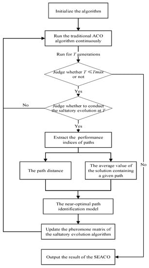
Figure 1. The SEACO algorithm flow chart.

5.1.1. The Path Performance Evaluation

The near-optimal paths in TSP refer to those paths that appear in the near-optimal solution. The continuous iterative optimization process of the ACO algorithm can be regarded as a process in which many ants constantly evaluate and adjust the path performance based on the past search experience to find the near-optimal paths. In this process, the path pheromone acts as a communication medium among ants, carrying and disseminating the path performance information shown in the past. Therefore, the cumulative pheromone of the path when the overall-optimal or near-optimal solution is found, is used to represent the path performance in this study.

Next, based on the traditional ACO algorithm mechanism, an index system for evaluating the path performance is proposed. As shown in Figure 2, the index system includes three aspects: (1) $d_{ij}$, the distance of the path (i, j). It represents the cost could be paid when ants moving through the given path, which is generally determined by the specific problem. (2) $f_{ij}\left(T\right)$, the selected frequency of path (i, j) in the first T generations. It is the frequency with which the given path is selected into the solution during the algorithm running process. (3) ${\overline{Z}}_{ij}\left(T\right)$, the average value of solution containing the path (i, j) in the first T generations. It describes the capability of the given path to be compatible with other paths to form a near-optimal solution. The specific calculation methods of index (2) and (3) are respectively shown in Formulas (5) and (6).

$${\overline{Z}}_{ij}\left(T\right)=\frac{{{\displaystyle \sum }}_m{{\displaystyle \sum }}_T{Z}_{ij}^{kt}}{C_{ij}}$$

(5)

$$f_{ij}\left(T\right)=\frac{C_{ij}}{m\ast T}$$

(6)

where $C_{ij}$ denotes the selected number of the path (i, j) during the first T iterations, and $Z_{ij}^{kt}$ refers to the solution value containing the path (i, j) of ant k at the t iteration. The larger the value of ${\overline{Z}}_{ij}\left(T\right)$, the weaker the capability of path (i, j) to be compatible with other paths to form a near-optimal solution, as the objective function of the TSP is to find the minimum value.

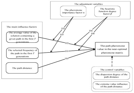
Figure 2. The conceptual diagram of the hypothesis test.

5.1.2. The Generation of the Near-Optimal Path Identification Rules

In this section, based on the path performance evaluation indicators proposed in Section 5.1.1, the quantitative analysis model is used to refine the TSP near-optimal path identification rule working as the domain knowledge to support the construction of the SEACO algorithm from the pheromone matrix evolution data of the traditional ACO algorithm.

At the initial moment of ACO, the pheromone of each path is the same, and the pheromone matrix is uniformly distributed. With the continuous iteration of the algorithm, the distribution of the pheromone matrix changes based on the search results and only one path is selected in each row of the pheromone matrix during each iteration of the TSP. In order to reflect the evolutionary trend of the pheromone matrix more clearly, the path pheromone is normalized in each row after each iteration. It is obvious that the total amount of path pheromones in each row of the pheromone matrix will converge to the near-optimal path when the algorithm achieves the global optimal solution. This matrix is defined as the near-optimal pheromone matrix in this study. In conclusion, the evolutionary process of the pheromone matrix is a process in which the path pheromone continuously converges from a uniform distribution to the near-optimal path. If the near-optimal path prediction rules can be found based on historical iterative data and be used to predict the future evolutionary trend of the pheromone matrix reasonably, it will greatly save the search time of the ACO algorithm and increase the convergence speed in this process.

Next, the quantitative analysis model will be used to test hypotheses, which is to mine the near-optimal path prediction rules from the pheromone matrix evolution data of the traditional ACO algorithm. First of all, each path pheromone in the near-optimal pheromone matrix is set as an explanatory variable Y, which describes the path performance, and then, three key assumptions that could affect the path pheromone in the near-optimal pheromone matrix are proposed based on the path performance evaluation indexes.

Hypothesis 0 (H0).

The larger the path distance, the smaller the path pheromone in the near-optimal pheromone matrix.

Hypothesis 1 (H1).

The larger the average value of the solution containing a given path, the smaller the path pheromone in the near-optimal pheromone matrix.

Hypothesis 2 (H2).

The higher the selected frequency of a given path, the larger the path pheromone in the near-optimal pheromone matrix.

It can be seen from Formula (2) that the pheromone importance factor α and the important factor of heuristic function β in the ACO algorithm affect the value of the path selection probability. Therefore, in the hypothesis test model, α and β are defined as the adjustment variables for the average value of the path solution and the frequency of path selection. The following four hypotheses are proposed based on the above algorithm mechanism:

Hypothesis 3 (H3).

The pheromone importance factor α can enhance the negative influence of the average value of the solution containing a given path on the path pheromone value in the near-optimal pheromone matrix.

Hypothesis 4 (H4).

The heuristic function degree factor β can weaken the negative influence of the average value of the solution containing a given path on the path pheromone value in the near-optimal pheromone matrix.

Hypothesis 5 (H5).

The pheromone importance factor α can enhance the positive influence of the selected frequency of a given path on the path pheromone value in the near-optimal pheromone matrix.

Hypothesis 6 (H6).

The heuristic function degree factor β can weaken the positive influence of the selected frequency of a given path on the path pheromone value in the near-optimal pheromone matrix.

Finally, the variance $S^2$ reflecting the dispersion degree of the paths distance in the TSP data sets and the index ΔE reflecting the influence of the extreme value of the path distance on the average value are added as control variables in the hypothesis test model as shown in Figure 2. The control variable ΔE is calculated with Formula (7), where $V_s$ refers to the vertex set of the graph G when removed top 10 edges with minimum distance, and $V_b$ denotes the vertex set of the graph G when removed top 10 edges with maximum distance.

$$\Delta \mathrm{E}=\frac{{{\displaystyle \sum }}_{i,j\in V_s}{d}_{ij}-{{\displaystyle \sum }}_{i,j\in V_b}{d}_{ij}}{N\ast N-10}$$

(7)

In order to verify the above hypotheses, 60% of the 79 data sets in international traveling salesman problem library (TSPLIB) database [20] were randomly selected as the training data sets, and the traditional ACO algorithm pheromone matrix evolution data in 200 generations were used to test the quantitative analysis model. The parameters of the traditional ACO algorithm according to previous research [21,22,23] were set as follows: the number of ants m was 50, the pheromone volatilization factor ρ was 0.1, the constant coefficient Q was 1, the maximum number of iterations was 200, and the running node T was 20. In addition, the pheromone value of the path (i, j) at the 200th generation was regarded as the estimated value of the path pheromone amount in the near-optimal pheromone matrix, so the regression equation is constructed as Formula (8).

$$\mathrm{y}=b_0+b_1{x}_1+b_2{x}_2+b_3{x}_3+b_4{x}_4+b_5{x}_5+b_6{x}_2{x}_4+b_7{x}_3{x}_4+b_8{x}_2{x}_5+b_9{x}_3{x}_5+b_{10}{x}_6+b_{11}{x}_7$$

(8)

where $x_1$ represents $d_{ij}, x_2$ stands for ${\overline{Z}}_{ij}\left(T\right), x_3$ denotes $f_{ij}\left(T\right),x_4$ is α (the value is 1 or 5), $x_5$ refers to β (the value is 2 or 5), $S^2$ is defined as $x_6,\mathrm{and}{x}_7$ stands for ΔE.

The results of quantitative analysis model test are shown in Table 1. The p-value of the regression equation is 0, which passes the significance test. The variance inflation factor (VIF) value of the regression equation without cross terms is equal to 6.3, indicating that there is no serious multicollinearity between variables. The regression coefficient of $x_1$ is negative, and the p-value is 0, indicating that the larger the path distance, the smaller the pheromone value of the path (i, j) in the near-optimal pheromone matrix. Therefore, the hypothesis H0 is supported. The regression coefficient of $x_2$ is positive indicating that the larger the average value of the solutions containing the path (i, j), the larger the pheromone value of path (i, j) in the near-optimal pheromone matrix, which is contrary to the original hypothesis H1. The evolutionary strategies in ACO algorithm to avoid the prematurity of pheromone matrix may be the reason, such as pheromone volatilization mechanism and roulette random selection strategy. The regression coefficient of $x_3$ is 0, indicating that the selected frequency of path (i, j) in the first T generations has no correlation with the pheromone value of path (i, j) in the near-optimal pheromone matrix. The hypothesis H2 is not supported, and thus, the hypothesis H5 and H6 about the adjustment variables are also not supported. What is more, the regression coefficient of the adjustment variable α is negative, and the regression coefficient of the cross term of α is also negative, indicating that α can weaken the positive effect of the average value of the solutions containing path (i, j) on the path pheromone value in the near-optimal pheromone matrix. Therefore, H3 is supported. The regression coefficient of the adjustment variable β is positive, but the regression coefficient of the cross term of β is negative, indicating that β can weaken the positive effect of the average value of the solutions containing path (i, j) on the path pheromone value in the near-optimal pheromone matrix, so H4 is supported. Finally, four near-optimal path identification rules are obtained, and the hypothesis test results are shown in Figure 3.

Table 1. The results of quantitative analysis model test.

Variable	Coefficient	p-Value
constant term	0.0018975	0 *
$x_1$	$-4.442\times {10}^8$	0 *
$x_2$	$8.1777\times {10}^{-10}$	$5.0679\times {10}^{-275}$ *
$x_3$	0	0 *
$x_4$	$-6.471\times {10}^{-6}$	0.00017177 *
$x_5$	$1.9936\times {10}^{-5}$	$3.4768\times {10}^{-13}$ *
$x_2{x}_4$	$-4.7122\times {10}^{-12}$	0.0015371 *
$x_3{x}_4$	0	0 *
$x_2{x}_5$	$-6.3676\times {10}^{-10}$	0 *
$x_3{x}_5$	0	0 *
$x_6$	$2.248\times {10}^{-12}$	0.19642
$x_7$	0.0017948	0 *
$R^2=0.00474, p-\mathrm{value}=0$

Notes: * represents p-value < 0.05. If p-value is under 0.05, the coefficient is statistically significant.

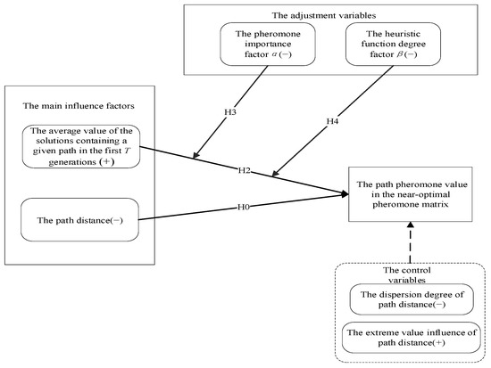
Figure 3. The results of the hypothesis test.

5.1.3. The Near-Optimal Path Identification

In this section, the adjustment variables α and β are fixed. The supported H0 and H2 are used to make a qualitative identification of the near-optimal path firstly, and then a model for predicting the near-optimal path is constructed to realize the saltatory evolution of the pheromone matrix of the traditional ACO algorithm and speed up the process of optimizing.

The qualitative identification process of the near-optimal path is as follows:

(a)

Discretizing variables.

All possible paths starting from i are considered as an analysis unit. Then variable $d_{ij}$ and variable ${\overline{Z}}_{ij}\left(T\right)$ are mapped to one of the low value interval $[\min \left(i\right),\frac{1}{3}(\max \left(i\right)+2 \min \left(i\right))]$, the median interval $\left(\frac{1}{3}\left(\max \left(i\right)+2\min \left(i\right)\right),\frac{1}{3}\left(2\max \left(i\right)+\min \left(i\right)\right)\right]$, and the high value interval $\left(\frac{1}{3}\left(2\max \left(i\right)+\min \left(i\right)\right),\max \left(i\right)\right]$ and are converted to the low, medium, and high value accordingly to be the discrete variables, where $\min \left(i\right)$ is the minimum variable value of all N possible paths starting from node i, and $\max \left(i\right)$ is the maximum variable value of all N possible paths starting from node i. It should be emphasized that the discretization will not be needed if ${\overline{Z}}_{ij}\left(T\right)$ is null.

(b)

Incorporating the identification rules and predicting the near-optimal path in different scenarios.

After the variables’ discretization, there would be 12 scenarios that are composed of different $d_{ij}$ and ${\overline{Z}}_{ij}\left(T\right)$, as shown in Table 2. It is assumed that the effect of one main variable will not completely offset the effect of another main variable, and the identification results are denoted by three grade variables, which are high, middle, and low value. When $d_{ij}$ belongs to a high level and ${\overline{Z}}_{ij}\left(T\right)$ belongs to a low level, the final judgment result is a low level because both main variables predict that the pheromone value of the path (i, j) in the near-optimal pheromone matrix will be a low level. In the same way, when $d_{ij}$ and ${\overline{Z}}_{ij}\left(T\right)$ are both at the middle level, the path (i, j) pheromone value in the near-optimal pheromone matrix is predicted to be at the middle level. When $d_{ij}$ is a low level and ${\overline{Z}}_{ij}\left(T\right)$ is a high level, the value of the path pheromone in the near-optimal pheromone matrix is predicted to be a high level. When ${\overline{Z}}_{ij}\left(T\right)$ is null, H2 will be invalid and the pheromone value of the path (i, j) in the near-optimal pheromone matrix is only judged according to $d_{ij}$ based on H0.

Table 2. The results of identification rules in different scenarios.

	${\overline{\mathit{Z}}}_{\mathit{i}\mathit{j}}\left(\mathit{T}\right)\mathbf{=}\mathbf{High}$	${\overline{\mathit{Z}}}_{\mathit{i}\mathit{j}}\left(\mathit{T}\right)\mathbf{=}\mathbf{Medium}$	${\overline{\mathit{Z}}}_{\mathit{i}\mathit{j}}\left(\mathit{T}\right)\mathbf{=}\mathbf{Low}$	${\overline{\mathit{Z}}}_{\mathit{i}\mathit{j}}\left(\mathit{T}\right)\mathbf{=}\mathbf{NAN}$
$d_{ij}$ = high	medium	low	low	low
$d_{ij}$ = medium	high	medium	low	medium
$d_{ij}$ = low	high	high	low	high

Notes: $d_{ij}$ is the path distance from city i to city j. ${\overline{Z}}_{ij}\left(T\right)$ refers to the average value of solution containing the path (i, j) in the first T generations.

(c)

Updating the pheromone matrix.

The high, low, and medium values of the qualitative identification results of the path pheromone respectively represent the increased, decreased, or unchanged evolutionary trend that the pheromone value of the path (i, j), namely, ${\tau }_{ij}\left(T\right)$, would show during the evolution of the pheromone matrix, and it is assumed that the change value of each path pheromone Q1 is fixed. According to Table 2, the qualitative pheromone matrix updating formula is obtained, as shown in Formula (9), where ${\tau }_{ij}^{\prime }$ is the prediction value of the path pheromone of (i, j).

$$\begin{array}{l}{\tau }_{ij}^{\prime }\\ =\{\begin{array}{c}{\tau }_{ij}+Q1,if \mathrm{the} \mathrm{pheromone} \mathrm{of} \mathrm{path}(i,j)\mathrm{in}\mathrm{the}\mathrm{near}-\mathrm{optimal}\mathrm{pheromone}\mathrm{matrix}\mathrm{is}\mathrm{high},\forall i,j\in V\\ {\tau }_{ij},\hspace{1em}if \mathrm{the} \mathrm{pheromone} \mathrm{of} \mathrm{path}(i,j)\mathrm{in}\mathrm{the}\mathrm{near}-\mathrm{optimal}\mathrm{pheromone}\mathrm{matrix}\mathrm{is}\mathrm{medium},\forall i,j\in V\\ {\tau }_{ij}-Q1,\hspace{1em}if \mathrm{the} \mathrm{pheromone} \mathrm{of} \mathrm{path}(i,j)\mathrm{in}\mathrm{the}\mathrm{near}-\mathrm{optimal}\mathrm{pheromone}\mathrm{matrix}\mathrm{is}\mathrm{low},\forall i,j\in V\end{array}\end{array}$$

(9)

(d)

The test of the qualitative identification rules.

In order to preliminarily verify the validity and applicability of the near-optimal path qualitative identification rules, 24 test data sets were used, and the experimental results were compared with the traditional ACO algorithm. First of all, in order to reasonably distinguish the different path performance from the pheromone value level, Q1 was selected as three values which are 0.1, 0.5, and 1 by observing the path pheromone value before updating. These three values could cover the change range of path pheromone and good simulation results would be relatively obtained through such parameter setting. Then, when the traditional ACO algorithm ran to the 20th generation, the pheromone matrix was updated with Formula (8). After updating, the ACO algorithm continued to run for one generation to output the optimized results. The average optimization result ${\overline{Y}}^{\prime }$. of the 24 data sets after the pheromone updating was compared with the average optimization result $\overline{Y}$ of the traditional ACO algorithm on the same data sets at the 20th generation so as to evaluate the effectiveness of the near-optimal path qualitative identification rules. Meanwhile, the optimization rate, that is, the proportion of the data sets with reduced running time after the application of the prediction rules in all experimental data sets, is used to evaluate the applicability of the near-optimal path qualitative identification rules. The experimental results are shown in Table 3. When Q1 is equal to 0.1, ${\overline{Y}}^{\prime }$ of 24 data sets is better than $\overline{Y}$, and the overall optimization rate reaches 41.67%. When Q1 is equal to 1, although ${\overline{Y}}^{\prime }$ of 24 data sets is not better than $\overline{Y}$, the overall optimization rate reaches 50%.

Table 3. The test results of qualitative prediction scheme.

Situation	Average Optimization Result of 24 Data Sets	Optimization Rate
the traditional ACO at the 20th generation	$1.015285551789795\times {10}^5$	-
Q1 = 0.5	$1.104654039153430\times {10}^5$	0
Q1 = 0.1	$1.014970895838640\times {10}^5$	0.4167
Q1 = 1	$1.019495374707328\times {10}^5$	0.5

Notes: Q1 is the change value of each path pheromone.

The experiment preliminarily confirms that the domain knowledge extracted in this study can effectively predict the evolutionary trend of the pheromone matrix. However, this experiment only used a qualitative method to make a rough discrete prediction of the near-optimal path. However, when the value of Q1 is 0.1, the average optimization results improved. While the optimization degree and optimization rate are not particularly prominent, this study further constructs a model for predicting the near-optimal path from a quantitative perspective to predict the near-optimal pheromone matrix continuously and improve performance of the SEACO algorithm.

The model of near-optimal path prediction is as follows:

(1)

Null variable treatment. When the $Z_{ij}\left(T\right)$ is null, $Z_{ij}\left(T\right)$ will be equal to $\frac{\max \left({\overline{Z}}_{ij}\left(T\right)\right)+\min \left({\overline{Z}}_{ij}\left(T\right)\right)}{2}$, so it is transformed into a continuous variable.

(2)

Construct the model for predicting the near-optimal path. Based on the verified Formula (9), the following model for predicting the near-optimal path is shown in Formula (10).

$${{\tau }^{\prime }}_{ij}={\tau }_{ij}\left(T\right)+\sin \left(\frac{\pi }{2}\ast \left(\frac{{\overline{Z}}_{ij}\left(T\right)-\min \left({\overline{Z}}_{ij}\left(T\right)\right)}{\max \left({\overline{Z}}_{ij}\left(T\right)\right)-\min \left({\overline{Z}}_{ij}\left(T\right)\right)}-\frac{d_{ij}-\min \left(d_i\right)}{\max \left(d_i\right)-\min \left(d_i\right)}\right)\right),\forall i,j\in V$$

(10)

where ${\tau }_{ij}\left(T\right)$ denotes the pheromone value of the path (i, j) at the Tth generation. ${\tau }_{ij}^{\prime }$ refers to pheromone prediction value of the path (i, j) in the near-optimal pheromone matrix. ${\overline{Z}}_{ij}\left(T\right)$ describes the average value of the solutions containing paths (i, j) before T generations. ${\overline{Z}}_{ij}\left(T\right)$ is a vector representing average values of the solutions, and each solution contains one path starting from i. $d_{ij}$ is defined as the distance of path (i, j) and $d_i$ symbolizes a vector which contains all the paths distance starting from i.

5.2. Steps of the SEACO Algorithm

As shown in Figure 1, the detailed steps of SEACO algorithm are as follows:

(1)

Initialize the algorithm.

Let the number of ants be m, pheromone importance factor be α, heuristic function important factor be β, pheromone volatilization factor be ρ, constant coefficient be Q, heuristic function be η, the maximum number of iterations be $T_{max}$ in the ACO algorithm and set the starting generation for operating the saltatory evolution.

(2)

Iterate for T times.

At the beginning of each iteration, m ants are randomly placed on the initial position. and the selection probability of each path is calculated by Formula (2). Then according to the roulette method, the path selection is completed one by one, and the values of m solutions are obtained and the solution with shortest distance is selected as the output of this iteration. Finally, the pheromone value of each path will be updated according to Formulas (4) and (5), and each row of the pheromone matrix is normalized. After updating the pheromone matrix, step 2 is repeated until the number of iterations T is equal to $T_{max}$, or T reaches the starting generation of the saltatory evolution.

(3)

Identify the near-optimal path and update the pheromone matrix.

When the number of iterations T reaches the starting generation of saltatory evolution, ${\overline{Z}}_{ij}\left(T\right)$, the average value of the solutions containing path (i, j), will be calculated according to Formula (5). Then ${\overline{Z}}_{ij}\left(T\right)$ and the path distance $d_{ij}$ will be input into the near-optimal path prediction model as shown in Formula (10) to update the pheromone matrix.

(4)

Conduct the saltatory evolution.

With other variables unchanged, run the traditional ACO algorithm using the updated pheromone matrix according to step 2. If the number of iterations T reaches $T_{max}$, the near-optimal solution of the last iteration will be output. Otherwise, judge whether T reaches the starting generation of saltatory evolution. If yes, repeat step 3. If not, go to step 2.

6. Experimental Results and Model Comparison

6.1. The Saving Generations of SEACO Algorithm Compared with Traditional ACO Algorithm

In order to verify the effectiveness of the SEACO algorithm in improving the optimization speed, the SEACO algorithm was compared with the traditional ACO algorithm in terms of the time complexity firstly. The asymptotic time complexity of the algorithm $T\left[n\right]$ is calculated by $O\left(f\left(n\right)\right)$ [24], where n denotes the input amount, $f\left(n\right)$ indicates the sum of the number of running each line of code, and O refers to the positive proportional relationship. Accordingly, the time complexity of the traditional ACO algorithm is O($n^2$). While the running time of the SEACO algorithm is $2n^2+n$, which is also O($n^2$) after ignoring the coefficients and low-power terms. Therefore, the SEACO algorithm does not increase the running time complexity of the traditional ACO algorithm, which means the time complexity of the two algorithms increases at the same rate with the increase of the input amount n.

Next, the experiment was run on 24 test data sets, which were randomly selected from the TSPLIB database, and these data sets were broadly representative because their city numbers ranged from 100 to 1379. The running time was compared when the SEACO algorithm and the traditional ACO algorithm got the same result. For example, if the near-optimal solution of the SEACO algorithm at the Tth generation is smaller than or equal to the near-optimal solution of the traditional ACO algorithm at the (T + t)th generation, it means that the SEACO algorithm saves t generations of running time than the traditional ACO algorithm. The experiment was applied on Matlab R2017b software with i7 Intel processor and 32GB internal storage. Based on the parameters of traditional ACO and other improved ACO algorithm [21,22,23], the following parameters of the SEACO algorithm were set. The number of ants m was 200; the pheromone importance factor α was 1; the heuristic function important factor β was 5; the pheromone volatilization factor ρ was 0.1, and the constant variable Q was 1. The SEACO algorithm was conducted with pheromone matrix updated at the 10th, 20th, 30th, 40th, 50th, 60th, 70th, 80th, 90th, and 100th generation of the traditional ACO algorithm, and continue running 3 generations after each update to find the best solution. The consumed generations for achieving the same solution are compared between the SEACO algorithm and the traditional ACO. The complete comparison results are shown in Table 4, and Figure 4 displays the data sets with the largest improvement in different injected generations.

Table 4. The saving generations of SEACO algorithm than ACO algorithm on the test data sets.

Data Sets	10th	20th	30th	40th	50th	60th	70th	80th	90th	100th
att532	12	41	31	21	11	4	0	0	0	0
d1291	12	29	19	9	0	1	6	0	0	0
d1655	22	32	22	12	10	0	3	3	7	0
d493	10	28	18	9	0	0	5	0	0	0
d657	30	20	10	0	10	0	2	1	0	0
fl1577	5	19	3	0	3	0	0	0	5	0
gil262	6	4	0	0	0	15	5	9	0	0
kroB200	0	27	15	7	0	2	12	2	7	0
kroC100	0	22	12	3	6	0	0	7	0	0
kroE100	13	3	1	10	0	0	3	1	7	0
nrw1379	20	34	27	15	7	1	0	0	1	0
p654	40	30	20	10	0	9	0	0	7	0
pa561	21	16	14	6	0	0	0	1	0	0
pcb1173	29	37	27	17	7	0	0	0	0	0
rat575	0	13	5	0	3	0	6	11	1	0
rat783	5	18	8	0	0	0	0	0	2	0
rd100	13	3	16	7	0	0	1	17	7	0
u1432	42	43	39	23	13	9	0	0	0	0
u1817	12	34	27	23	3	0	0	0	1	0
u574	21	28	25	23	5	0	2	3	2	0
u724	9	28	20	10	6	0	4	4	0	0
rl1304	49	39	29	30	20	14	0	3	0	0
rl1323	45	52	48	32	22	12	2	0	0	0
u1060	6	48	48	40	28	12	4	0	0	0
Mean	17.6	27	20.2	12.8	6.4	3.3	2.3	2.6	2	0
Max	49	52	48	40	28	15	12	17	7	0
Optimization rate	0.88	1	0.96	0.80	0.63	0.42	0.54	0.50	0.46	0

Notes: 10th means the SEACO algorithm conducts the saltatory evolution at the 10th generation and so on.

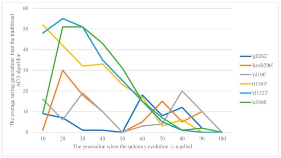
Figure 4. The saving generations of SEACO algorithm on test data sets.

As shown in Table 4, the optimization rate of the SEACO algorithm on the test data sets is over 46% before 90th generation, and over 80% before 40th generation. This indicates that the SEACO algorithm has wide applicability and effectiveness on approximating TSPs with limited time window. Moreover, it can be seen from Figure 4 that the earlier the SEACO algorithm is conducted, the faster the optimization speed is improved. Specifically, the SEACO algorithm performs best at the 20th generation with 100% optimization rate, and 52 generations can be saved at most, and 27 generations can be saved on average. However, the performance of the SEACO algorithm has not been improved at the 100th generation, which indicates that the SEACO algorithm is more suitable to be injected into the ACO algorithm in the early stage, and the quantitative analysis model for identifying the near-optimal path needs to be reconstructed so as to continue accelerating the traditional ACO algorithm after the 100th generation.

In order to further verify the wide applicability of the SEACO algorithm, the experiment was also run on all 79 TSP data sets, and the average saving generations of the SEACO algorithm are shown in Table 5. These data sets were divided into five groups according to their city scales, where the number of cities n lies in (0, 100], (100, 200], (200, 400), [400, 800], and (800, 2000], respectively. Then, the optimized performance of the SEACO algorithm on different data sets with different city scales are compared, and the data sets with the largest improvement in different injected generations are shown in Figure 5, Figure 6, Figure 7, Figure 8 and Figure 9.

Table 5. The average saving generations of SEACO algorithm than ACO algorithm on all data sets.

Data Sets	10th	20th	30th	40th	50th	60th	70th	80th	90th	100th
(0, 100]	13.2	20	17.7	21	18.9	18.8	14	14.4	7	0
(100, 200]	11.2	15.5	12.5	13.3	9.7	5.6	7	6.9	4.8	0
(200, 400)	16.7	18.1	12.3	10.5	5.9	8.2	5.8	9.7	5.4	0
[400, 800]	19.2	23.7	15.8	10.9	4.7	2.4	1.9	3.5	2.6	0
(800, 2000]	31.6	39.3	33.2	25	15.5	6.3	2	0.3	1.3	0
all data sets	18.38	23.32	18.3	16.14	10.94	8.26	6.14	6.96	4.22	0
optimization rate of all data sets	0.80	0.85	0.90	0.80	0.70	0.53	0.53	0.60	0.68	0

Notes: (0, 100] represents data sets where n is in (0, 100] and so on.

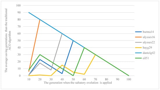
Figure 5. The optimization results of SEACO algorithm for data sets where n is in (0, 100].

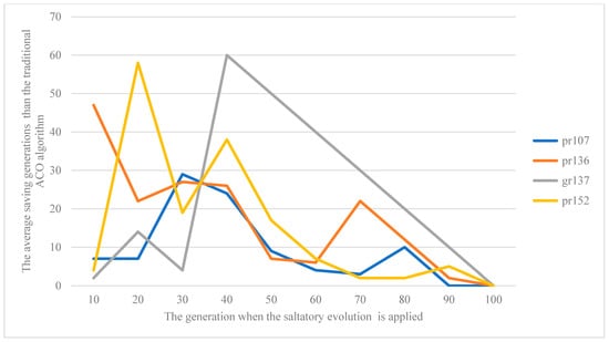
Figure 6. The optimization results of SEACO algorithm for data sets where n is in (100, 200].

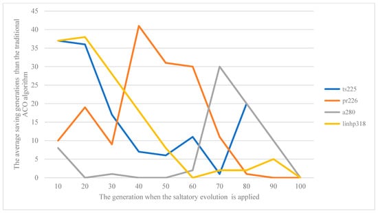
Figure 7. The optimization results of SEACO algorithm for data sets where n is in (200, 400).

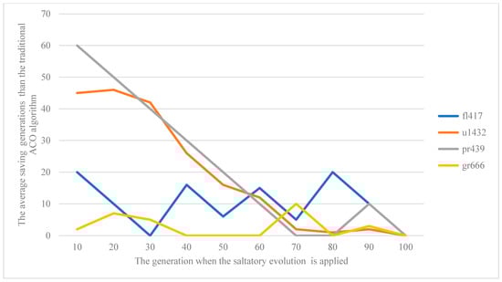
Figure 8. The optimization results of SEACO algorithm for data sets where n is in [400, 800].

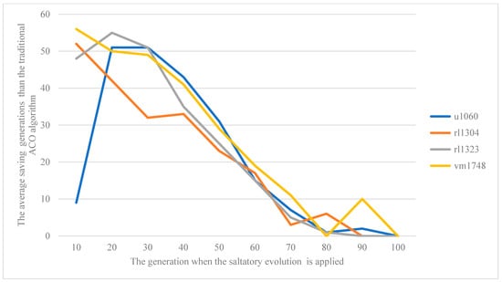
Figure 9. The optimization results of SEACO algorithm for data sets where n is in (800, 2000].

The results shown in Table 5 present the optimization rate of the SEACO algorithm before 90th generation is over 68% on all 79 TSP data sets and over 80% before 40th generation. This means that the SEACO algorithm can be widely applied on different TSP.

It can be seen from Table 5 that the SEACO algorithm performs best in the first group of city data sets where n is in (100, 200]. Specifically, it can be seen from Figure 5 that the SEACO algorithm achieves the best performance on the data sets named dantzig42 at the 10th generation, whose optimization result is equivalent to the traditional ACO algorithm at the 100th generation, and 87 generations of running time are saved. In addition, the SEACO algorithm on the data sets of ulysses16, burma14, ulysses22, and eil51 also respectively shows the best performance when the SEACO injected at the 30th, 40th, and 50th generations, and saved 67, 57, 47, and 37 generations of running time separately.

As shown in Figure 5, Figure 6, Figure 7, Figure 8 and Figure 9, the optimization ability of the SEACO algorithm presents a decreased trend with the delay of injection time on all city-scale data sets, which means it can slightly improve the optimization speed when injected in the earlier running stage. As shown in Figure 10, the SEACO algorithm reflects better performance on the larger scale data sets than the smaller one in general. Specifically, the SEACO algorithm performs best in the data sets where the city number is within (800, 2000], and nearly 40 generations on average can be saved when injected at the 20th generation. This means that the SEACO algorithm can significantly improve the optimization speed of the large-scale TSP.

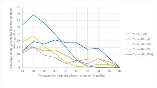
Figure 10. The average optimization results of SEACO algorithm on different data groups.

Finally, in order to investigate the performance of the SEACO algorithm under different conditions of the control variables, the average optimization results are compared in different situation. Firstly, the data sets are divided into five groups by mapping the path distance variances $S^2$ into (0, 1000), (1000, 100,000), (100,000, 1,000,000), (1,000,000, 100,000,000), or (100,000,000, 200,000,000) interval, and the average optimization results on these groups are shown in Figure 11. It can be seen that there is no significant difference on optimization results among these groups with different path distance variances. Next, the data sets are divided into four groups by mapping ΔE into (0.001, 0.01), (0.01, 0.1), (0.1, 1), or (1, 21) interval, and the results are shown in Figure 12. It can be found that the SEACO algorithm performs more prominently in the data sets with smaller ΔE than the data set with larger ΔE. This implies that the SEACO algorithm is more suitable for the TSP whose extreme value of the path distance has a small influence on the average value of the path distance.

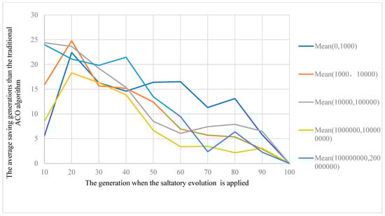
Figure 11. The classified statistics of path distance dispersion.

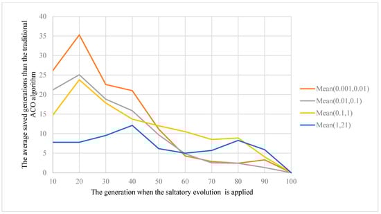
Figure 12. The classified statistics of the extreme influence of path distance.

6.2. The Comparison with Other Improved Algorithms

On the one hand, this study compares SEACO and other improved ACO algorithms such as the parallel-ranking ant colony optimization (PRACO) [3] and ACO for enhancing the negative feedback mechanism (ACON) [17] algorithm to further prove the effectiveness of the SEACO algorithm. First, the time complexity of PRACO and ACON is the same as SEACO. Then, the solution qualities of three algorithms are compared under the same time window (running 23 generations), as shown in Table 6. The parameters are the same as the above experiments in Section 6.1, the PRACO algorithm includes three ant subgroups, and the total number of ants is 200.

Table 6. The target value of SEACO algorithm compared with other improved algorithms.

Value Excess	Data Sets	Best Target Value	Average Target Value	Worst Target Value
SEACO-PRACO	(0, 100]	−810.99	−130.93	3.85
	(100, 200]	−4666.54	−687.10	2397.09
	(200, 400)	−8854.31	−1675.57	40.09
	[400, 800]	−2414.67	−308.71	0.00
	(800, 2000]	−34,799.82	−13,577.59	−2362.92
	all data sets average	−10,309.27	−3275.98	15.62
SEACO-ACON	(0, 100]	−4921.54	−300.96	704.05
	(100, 200]	−5639.19	−573.60	973.32
	(200, 400)	−7829.89	−1633.28	16.33
	[400, 800]	−11,239.99	−2767.47	175.87
	(800, 2000]	−27,514.66	−12,354.15	−1519.72
	all data sets average	−11,429.05	−3525.89	69.97
(RNN-SEACO)-RNN	(0, 100]	−22,771.54	−2699.50	−24.68
	(100, 200]	−14,072.58	−2058.86	0.00
	(200, 400)	−3326.52	−458.44	0.00
	[400, 800]	−12,997.75	−2666.25	599.16
	(800, 2000]	0.00	0.00	0.00
	all data sets average	−10,633.678	−1576.61	114.896

Notes: (0, 100] represents data sets where n is in (0, 100] and so on.

As shown in Table 6, the solution quality of SEACO is the best when running the same generations. Among all the TSP data sets, the SEACO algorithm shows a better solution quality than the PRACO algorithm on 87.34% of TSP data sets, with an average reduction of 3275.98. Meanwhile, the SEACO algorithm has a better solution quality than the ACON algorithm on 79.75% of TSP data sets, with an average reduction of 3525.89.

On the other hand, in order to further verify the effectiveness of the improvement measures of the SEACO algorithm, the RNN-SEACO algorithm is designed based on RNN, as RNN is an algorithm with high solution quality at present [25]. The main idea of the RNN-SEACO algorithm is that in the first generation of the SEACO algorithm, one solution is generated by the RNN algorithm, and the other solutions are randomly generated by the pheromone matrix. At the same time, the optimal solution generated up to the current generation is retained in each generation. The idea of RNN is to start with a tour of k nodes, where k is the number of vertices that make up the partial tours, and then perform a Nearest-Neighbor search from there on. After doing this for all permutations of k nodes, the result gets selected as the shortest tour found [26].

The comparison of target values between RNN-SEACO and RNN algorithms when running 23 generations is shown Table 6. The k of RNN is 2, and other parameters and TSP data sets are the same as above. It can be seen from Table 6 that the RNN-SEACO algorithm is able to reduce the target value of 22,771.54 at most and can reduce the target value of 1576.61 on average. This shows that the mechanism of saltatory evolution proposed by this study can get a satisfactory solution on the basis of RNN.

In summary, the effectiveness and wide applicability of the SEACO algorithm are verified in various TSP data sets. At the same time, the SEACO algorithm can better accelerate the optimization speed in the early stage of the traditional ACO algorithm and is more applicable to approximate large-scale TSP with limited time window, which can provide a promising direction to improve searching speed of the traditional ACO algorithm on large-scale combination optimization. In addition, the comparison with other improved ACO algorithms indicates that the solution quality of the SEACO algorithm is much better, which also verifies its effectiveness and applicability. In addition, adding the results of the RNN algorithm to the initial solution of the SEACO algorithm can approach the global optimal solution more efficiently.

7. Conclusions

In order to overcome the shortcoming of long optimization time of the traditional ACO algorithm, this study constructs a new type of fast-approximating ACO algorithm—the SEACO algorithm, which is constructed in three stages, namely, the path performance evaluation stage, the near-optimal path identification rules generation stage, and the near-optimal path identification stage from the perspective of near-optimal path identification. Then the SEACO algorithm is compared with the traditional ACO algorithm and other improved ACO algorithms on the TSPLIB, respectively. On the test data sets, the optimization rate of SEACO algorithm is above 46% before the 90th generation, and it achieves 100% optimization rate when injected at the 20th generation with 52 generations saved at most and 27 generations saved on average. On all 79 data sets, the optimization rate of the SEACO algorithm is over 68% before the 90th generation, and it reaches 90% when SEACO is injected at the 30th generation, and on average 17 generations and maximum 77 generations time are saved. This fully verifies that the SEACO algorithm proposed in this study can effectively improve the approximating speed and can be widely applied to various TSPs with a limited time window. What is more, an excellent performance can be obtained when the SEACO algorithm is injected into the traditional ACO algorithm in earlier stage. In terms of the solution quality, the SEACO algorithm shows a better solution quality than the PRACO algorithm on 87.34% TSP data sets, with an average reduction of 3275.98, and it has a better solution quality than the ACON algorithm on 79.75% TSP data sets, with an average reduction of 3525.89. The comparison from different city scales of the data sets reveals that the SEACO algorithm can save more running time on the larger scale TSP data sets. This means it can provide a promising direction to deal with the problem of slow optimization speed of the traditional ACO algorithm and better improve the solution quality than other improved ACO algorithms. In addition, after using the RNN algorithm to update the initial solution, the global optimal solution can be approached more effectively.

This study also has the following limitations. Firstly, the SEACO algorithm is injected only once to accelerate the optimization speed. The optimization efficiency of multiple injections of the SEACO algorithm will be investigated in the future. In addition, the performance of multiple injections is expected to achieve continuous acceleration and effectively avoid the ACO algorithm from falling into local optimal solutions. Secondly, this study mainly focuses on obtaining a good solution in a short time, neglecting to search the global optimal solution. How to approximate TSP quickly as well as effectively with the SEACO algorithm will be studied in the future. Finally, the SEACO algorithm can be applied to some other practical optimization problems so as to further verify its effectiveness and wide applicability.

References

- Dorigo, M.; Maniezzo, V.; Colorni, A. Positive Feedback as a Search Strategy. June 1991. Available online: http://citeseerx.ist.psu.edu/viewdoc/summary?doi=10.1.1.52.6342 (accessed on 14 January 2022).
- Dorigo, M.; Birattari, M.; Stutzle, T. Ant colony optimization. IEEE Comput. Intell. Mag. 2006, 1, 28–39. [Google Scholar] [CrossRef]
- Yu, J.; Li, R.; Feng, Z.; Zhao, A.; Yu, Z.; Ye, Z.; Wang, J. A Novel Parallel Ant Colony Optimization Algorithm for Warehouse Path Planning. J. Control Sci. Eng. 2020, 2020, 5287189. [Google Scholar] [CrossRef]
- Tomanova, P.; Holy, V. Ant Colony Optimization for Time-Dependent Travelling Salesman Problem. In Proceedings of the 4th International Conference on Intelligent Systems, Metaheuristics and Swarm Intelligence (ISMSI)/India International Congress on Computational Intelligence (IICCI), Thimphu, Bhutan, 18–19 April 2020; pp. 47–51. [Google Scholar]
- Lucky, L.; Girsang, A.S. Hybrid Nearest Neighbors Ant Colony Optimization for Clustering Social Media Comments. Informatica 2020, 44, 63–74. [Google Scholar] [CrossRef] [Green Version]
- Yin, C.; Li, T.; Qu, X.; Yuan, S. An Improved Ant Colony Optimization Job Scheduling Algorithm in Fog Computing. In Proceedings of the International Symposium on Artificial Intelligence and Robotics, Kitakyushu, Japan, 8–10 August 2020; Volume 11574, p. 115740G. [Google Scholar] [CrossRef]
- Zannou, A.; Boulaalam, A.; Nfaoui, E.H. Relevant node discovery and selection approach for the Internet of Things based on neural networks and ant colony optimization. Pervasive Mob. Comput. 2021, 70, 101311. [Google Scholar] [CrossRef]
- Yu, J.; You, X.; Liu, S. Dynamic Density Clustering Ant Colony Algorithm With Filtering Recommendation Backtracking Mechanism. IEEE Access 2020, 8, 154471–154484. [Google Scholar] [CrossRef]
- Dai, X.; Long, S.; Zhang, Z.; Gong, D. Mobile Robot Path Planning Based on Ant Colony Algorithm With A(*) Heuristic Method. Front. Neurorobot. 2019, 13, 15. [Google Scholar] [CrossRef] [PubMed]
- Zheng, F.; Zecchin, A.C.; Newman, J.P.; Maier, H.R.; Dandy, G.C. An Adaptive Convergence-Trajectory Controlled Ant Colony Optimization Algorithm With Application to Water Distribution System Design Problems. IEEE Trans. Evol. Comput. 2017, 21, 773–791. [Google Scholar] [CrossRef]
- Chen, X.; Dai, Y. Research on an Improved Ant Colony Algorithm Fusion with Genetic Algorithm for Route Planning. In Proceedings of the 4th IEEE Information Technology, Networking, Electronic and Automation Control Conference (ITNEC), Electr Network, Chongqing, China, 12–14 June 2020; pp. 1273–1278. [Google Scholar]
- Gao, S.; Wu, J.; Ai, J. Multi-UAV reconnaissance task allocation for heterogeneous targets using grouping ant colony optimization algorithm. Soft Comput. 2021, 25, 7155–7167. [Google Scholar] [CrossRef]
- Zhang, S.; Pu, J.; Si, Y. An Adaptive Improved Ant Colony System Based on Population Information Entropy for Path Planning of Mobile Robot. IEEE Access 2021, 9, 24933–24945. [Google Scholar] [CrossRef]
- Deng, W.; Xu, J.; Song, Y.; Zhao, H. An effective improved co-evolution ant colony optimisation algorithm with multi-strategies and its application. Int. J. Bio-Inspired Comput. 2020, 16, 158–170. [Google Scholar] [CrossRef]
- Pan, H.; You, X.; Liu, S.; Zhang, D. Pearson correlation coefficient-based pheromone refactoring mechanism for multi-colony ant colony optimization. Appl. Intell. 2021, 51, 752–774. [Google Scholar] [CrossRef]
- Wei, X. Task scheduling optimization strategy using improved ant colony optimization algorithm in cloud computing. J. Ambient Intell. Humaniz. Comput. 2020, 1–12. [Google Scholar] [CrossRef]
- Li, J.; Xia, Y.; Li, B.; Zeng, Z. A pseudo-dynamic search ant colony optimization algorithm with improved negative feedback mechanism. Cogn. Syst. Res. 2020, 62, 1–9. [Google Scholar] [CrossRef]
- Gao, W. New ant colony optimization algorithm for the traveling salesman problem. Int. J. Comput. Intell. Syst. 2020, 13, 44–55. [Google Scholar] [CrossRef] [Green Version]
- Lipowski, A.; Lipowska, D. Roulette-wheel selection via stochastic acceptance. Phys. A Stat. Mech. Appl. 2012, 391, 2193–2196. [Google Scholar] [CrossRef] [Green Version]
- Reinelt, G. TSPLIB—A Traveling Salesman Problem Library. ORSA J. Comput. 1991, 3, 376–384. [Google Scholar] [CrossRef]
- Duan, H.B.; Ma, G.J.; Liu, S.Q. Experimental study of the adjustable parameters in basic ant colony optimization algorithm. In Proceedings of the 2007 IEEE Congress on Evolutionary Computation, Singapore, 25–28 September 2007; pp. 149–156. [Google Scholar] [CrossRef]
- Li, Z.; Chen, X.; Wang, H. Modified ACO for General Continuous Function Optimization. In Proceedings of the 2012 Second International Conference on Intelligent System Design and Engineering Application, Sanya, China, 6–7 January 2012; pp. 348–354. [Google Scholar]
- Hong, W.-C.; Dong, Y.; Zheng, F.; Lai, C.-Y. Forecasting urban traffic flow by SVR with continuous ACO. Appl. Math. Model. 2011, 35, 1282–1291. [Google Scholar] [CrossRef]
- Jasser, M.B.; Sarmini, M.; Yaseen, R. Ant Colony Optimization (ACO) and a Variation of Bee Colony Optimization (BCO) in Solving TSP Problem: A Comparative Study. Int. J. Comput. Appl. 2014, 96, 1–8. [Google Scholar]
- Chauhan, A.; Verma, M. 5/4 approximation for Symmetric TSP. arXiv 2019, arXiv:1905.05291. [Google Scholar]
- Klug, N.; Chauhan, A.; Ragala, R. k-RNN: Extending NN-heuristics for the TSP. Mob. Netw. Appl. 2019, 24, 1210–1213. [Google Scholar] [CrossRef] [Green Version]
Publisher’s Note: MDPI stays neutral with regard to jurisdictional claims in published maps and institutional affiliations. |
© 2022 by the authors. Licensee MDPI, Basel, Switzerland. This article is an open access article distributed under the terms and conditions of the Creative Commons Attribution (CC BY) license (https://creativecommons.org/licenses/by/4.0/).