An Inertial Extragradient Direction Method with Self-Adaptive Step Size for Solving Split Minimization Problems and Its Applications to Compressed Sensing

Abstract

The purpose of this work is to construct iterative methods for solving a split minimization problem using a self-adaptive step size, conjugate gradient direction, and inertia technique. We introduce and prove a strong convergence theorem in the framework of Hilbert spaces. We then demonstrate numerically how the extrapolation factor $\left({\theta }_n\right)$ in the inertia term and a step size parameter affect the performance of our proposed algorithm. Additionally, we apply our proposed algorithms to solve the signal recovery problem. Finally, we compared our algorithm’s recovery signal quality performance to that of three previously published works.

1. Introduction

Let C and Q be two closed convex subsets of two real Hilbert spaces ${\mathcal{H}}^1$ and ${\mathcal{H}}^2$, respectively, and denote the metric projection onto C by ${\mathrm{Proj}}_C$. Assume that A is a bounded linear operator and that $A^{*}$ is its adjoint operator.

In 1994, Censor and Elfving [1] defined the split feasibility problem (SFP) as

$$\begin{array}{c}\hfill \mathrm{finding}{x}^{*}\in C\mathrm{such}\mathrm{that}A{x}^{*}\in Q.\end{array}$$

(1)

This problem was designed to model inverse problems, which are at the core of many real-world problems, such as phase retrieval, image restoration, and intensity-modulated radiation therapy (IMRT). Specifically, signal processing, including signal recovery, which is used to transmit data in almost every field imaginable. Signal processing is essential for the use of X-rays, MRIs, and CT scans, as it enables complex data processing techniques to analyze and decipher medical images. As a result, a great amount of research is motivated to solve the SFP (1). See [2,3,4].

Berny [5] popularized the CQ algorithm for finding the SFP (1) solution. This algorithm is based on the fixed-point concept:

$$\begin{array}{c}\hfill {\mathrm{Proj}}_C(I-{\kappa }_n{A}^{*}(I-{\mathrm{Proj}}_Q)A)x^{*}=x^{*},\end{array}$$

(2)

where ${\kappa }_n$ is a constant. Other iterative methods for resolving the split feasibility problem (1) are described in [6,7,8,9,10,11,12,13] and its references. However, we needed prior knowledge of matrix norm A in order to use these iterative methods.

Yang [14] proposed the relaxed CQ algorithm in 2005 to avoid computing the operator norm of a bounded linear operator, but this algorithm remains subject to many conditions. As a result, many researchers have proposed and studied self-adaptive step size algorithms to obtain fewer conditions. Further information is available from [15,16,17,18].

López [18] introduced the intriguing self-adaptive step size algorithm in 2012, which is worth further investigation. This algorithm generates sequence $\left\{x_n\right\}$ in the following manner:

$$\begin{array}{ccc}\hfill {\kappa }_n& =& {\displaystyle \frac{{\varrho }_n\omega \left(x_n\right)}{\parallel \nabla \omega \left(x_n\right)\parallel }},\hfill \\ \hfill x_{n+1}& =& {\mathrm{Proj}}_C(I-{\kappa }_n{A}^{*}(I-{\mathrm{Proj}}_Q)A)x_n,n\ge 1,\hfill \end{array}$$

(3)

where $x_1\in {\mathcal{H}}^1$ is arbitrarily selected, $\omega \left(x\right)=\parallel (I-{\mathrm{Proj}}_Q){Ax\parallel }^2/2$ is the convex objective function and $\nabla \omega \left(x\right)=A^{*}(I-{\mathrm{Proj}}_Q)Ax$ is its Lipschitz gradient, and $\left\{{\varrho }_n\right\}$ is a sequence satisfying $0<{\varrho }_n<4$ and $inf{\varrho }_n(4-{\varrho }_n)>0.$

We now describe the variational inequality problem (VIP), as variational inequality theory is a major necessity for studying a broader class of numerous problems that arise in wide variety of fields of the pure and applied sciences. Assume that $p:{\mathcal{H}}^1\to {\mathcal{H}}^1$ is a monotone operator. The VIP is defined mathematically as follows:

$$\begin{array}{c}\hfill \mathrm{find}{x}^{*}\in C\mathrm{such}\mathrm{that}⟨p\left(x^{*}\right),x-x^{*}⟩\ge 0.\end{array}$$

(4)

The projected gradient method [19] is the simplest iterative method for solving the VIP. This algorithm generates sequence $\left\{x_n\right\}$ in the following fashion:

$$\begin{array}{ccc}\hfill x_{n+1}& =& {\mathrm{Proj}}_C(I-{\kappa }_{n}p)x_n,n\ge 1,\hfill \end{array}$$

(5)

where $x_1\in {\mathcal{H}}^1$ is arbitrarily selected and ${\kappa }_n$ is a positive real number. However, to use the projected gradient method, we must know the closed-form expression of the metric projection ${\mathrm{Proj}}_C$, which does not always exist. As a result, the steepest descent algorithms have been introduced and further developed in recent years. Following that, methods for accelerating the steepest descent method have been constructed and developed. When $p:C\to \mathbb{R}$ is a convex function that is also Fréchet differentiable, the conjugate gradient direction [20] of h at $x_n$ is defined as follows:

$$\begin{array}{ccc}\hfill d_1& =& -\nabla p\left(x_1\right),\hfill \\ \hfill d_{n+1}& =& -\nabla p\left(x_n\right)+b_n{d}_n,n\ge 1,\hfill \end{array}$$

(6)

where $x_1\in C$ is arbitrarily selected, $b_n$ is a sequence satisfying $0<b_n<\infty$, and $\nabla p$ is the gradient of function p.

Sakurai and Iiduka [21] investigated and introduced the iterative method to solve a fixed point of a nonexpansive mapping. This method is based on the concept of conjugate gradient directions (6), which can be used to accelerate the steepest descent method, which generates the sequence $\left\{x_n\right\}$ as follows:

$$\begin{array}{ccc}\hfill d_1& =& \frac{(S-I)x_1}{\alpha },\hfill \\ \hfill d_{n+1}& =& \frac{(S-I)x_n}{\alpha }+b_n{d}_n,\hfill \\ \hfill y_n& =& x_n+\alpha d_{n+1},\hfill \\ \hfill x_{n+1}& =& \mu {\alpha }_n{x}_n+(1-\mu {\alpha }_n)y_n,n\ge 1,\hfill \end{array}$$

(7)

where $x_1\in C$ is arbitrarily selected, S is a nonexpansive mapping on C, $\alpha >0$, $\mu$ is a constant satisfying $0\le \mu <1$, $\left\{{\alpha }_n\right\}$ is a sequence in $(0,1)$, and $\left\{b_n\right\}$ is a sequence satisfying $0\le b_n<\infty$. The strong convergent theorem was established by Sakurai and Iiduka. Additionally, they demonstrated the performance of their algorithm, which significantly reduced the time required to find a solution.

Additionally, numerous researchers have concentrated their efforts on accelerating the convergence rate of algorithms. Polyak [22] pioneered this concept by introducing the heavy ball method, a critical technique for increasing the convergence rate of algorithms. Following that, modified heavy ball methods were introduced and developed to accelerate their algorithm convergence rate. Nesterov [23] introduced one of the most versatile modified heavy ball methods, which is defined as follows:

$$\begin{array}{ccc}\hfill y_n& =& x_n+{\theta }_n(x_n-x_{n-1}),\hfill \\ \hfill x_{n+1}& =& y_n+{\kappa }_n\nabla p\left(y_n\right),n\ge 2,\hfill \end{array}$$

(8)

where $x_1,x_2\in {\mathcal{H}}^1$ are arbitrarily selected, ${\kappa }_n$ is a positive constant, ${\theta }_n$ is an extrapolation factor satisfying $0\le {\theta }_n<1$, and the term ${\theta }_n(x_n-x_{n-1})$ is referred to as inertia. For additional information, the reader can consult [24,25,26].

Consider two proper, convex, and lower-semicontinuous functions, $f:{\mathcal{H}}^1\to \mathbb{R}$ and $g:{\mathcal{H}}^2\to \mathbb{R}$. Recently, Moudafi and Thakur [9] published an interesting paper on the split proximal feasibility problem, that is to find $x^{*}$ such that

$$\begin{array}{c}\hfill \underset{x^{*}\in {\mathcal{H}}^1}{min}\{f\left(x^{*}\right)+g_{\lambda }\left(A{x}^{*}\right)\},\end{array}$$

(9)

where $\lambda$ is a positive constant, and $g_{\lambda }\left(A{x}^{*}\right)={min}_{y\in {\mathcal{H}}^2}\{g\left(y\right)+{\displaystyle \frac{1}{2\lambda }}\parallel y-A{x}^{*}\parallel \}$ is the Moreau–Yosida approximation.

This problem is important for future work such as algorithms for designing large dimensional equiangular tight frames, additive parameters for deep face recognition, deep learning methods for compressed sensing, a unit softmax with Laplacian, and water allocation optimization. See, e.g., [27,28].

As can be seen, Rockafella [29] defined the subdifferential of the Moreau–Yosida approximation as follows:

$$\begin{array}{ccc}\hfill \partial (f\left(x^{*}\right)+g_{\lambda }\left(A{x}^{*}\right))& =& \partial f\left(x^{*}\right)+A^{*}\nabla g_{\lambda }\left(A{x}^{*}\right)\hfill \\ & =& \partial f\left(x^{*}\right)+A^{*}\left({\displaystyle \frac{I-{\mathrm{prox}}_{\lambda g}}{\lambda }}\right)\left(A{x}^{*}\right).\hfill \end{array}$$

(10)

Equation (10) implies that the following inclusion problem is optimal for the problem (9):

$$\begin{array}{c}\hfill 0\in \lambda \partial f\left(x^{*}\right)+A^{*}(I-{\mathrm{prox}}_{\lambda g})\left(A{x}^{*}\right),\end{array}$$

(11)

where ${\mathrm{prox}}_{\lambda g}\left(A{x}^{*}\right)=arg{min}_{y\in {\mathcal{H}}^2}\{g\left(y\right)+{\displaystyle \frac{1}{2\lambda }}\parallel y-A{x}^{*}\parallel \}$ is the proximity operator of function g order $\lambda$ and $\partial f\left(x^{*}\right)=\{\overline{x}\in {\mathcal{H}}^1:f\left(u\right)\ge f\left(x^{*}\right)+⟨\overline{x},u-x^{*}⟩,\forall u\in {\mathcal{H}}^1\}$ is the subdifferential of function f at the point $x^{*}$.

The problem (9) is referred to as the split minimization problem (SMP) when $argminf\cap A^{-1}argming\ne \varnothing$. It was defined by Moudafi and Thakur [9] as finding a point

$$\begin{array}{c}\hfill x^{*}\in argminf\mathrm{such}\mathrm{that}A{x}^{*}\in argming.\end{array}$$

(12)

where $argminf=\{\tilde{x}\in {\mathcal{H}}^1:f\left(\tilde{x}\right)\le f\left(x\right),\forall x\in {\mathcal{H}}^1\}$ and $argming=\{\tilde{y}\in {\mathcal{H}}^2:g\left(\tilde{y}\right)\le g\left(y\right),\forall y\in {\mathcal{H}}^2\}$. The significance of this problem is that it is a generalization of the SFP (1), as the SMP (12) can be reduced to the SFP (1) by setting functions f and g to be the indicator functions of the nonempty closed convex subsets C and Q, respectively.

Assume that   

$$\begin{array}{ccc}\hfill p\left(x\right)& =& {\displaystyle \frac{1}{2}}{\parallel (I-{\mathrm{prox}}_{\lambda g})Ax\parallel }^2,\hfill \end{array}$$

(13)

$$\begin{array}{ccc}\hfill q\left(x\right)& =& {\displaystyle \frac{1}{2}}{\parallel (I-{\mathrm{prox}}_{\lambda {\kappa }_{n}f})x\parallel }^2.\hfill \end{array}$$

(14)

The gradients of functions p and q are obtained as follows:

$$\begin{array}{ccc}\hfill \nabla p\left(x\right)& =& A^{*}(I-{\mathrm{prox}}_{\lambda g})Ax,\hfill \end{array}$$

(15)

$$\begin{array}{ccc}\hfill \nabla q\left(x\right)& =& (I-{\mathrm{prox}}_{\lambda {\kappa }_{n}f})x.\hfill \end{array}$$

(16)

We can verify that p and q are weakly lower semicontinuous, convex, and differentiable; see [30].

Abbas and Alshahrani [31] published two iterative algorithms in 2018 for determining the minimum-norm solution to a split minimization problem. These algorithms are denoted by the following formulas:

$$\begin{array}{ccc}\hfill {\tau }_n& =& {\varrho }_n\frac{p\left(x_n\right)+q\left(x_n\right)}{\sqrt{\parallel \nabla p\left(x_n\right){\parallel }^2+{\parallel \nabla q\left(x_n\right)\parallel }^2}},\hfill \\ \hfill x_{n+1}& =& {\mathrm{prox}}_{\lambda {\kappa }_{n}f}((1-{ϵ}_n)x_n-{\kappa }_n{A}^{*}(I-{\mathrm{prox}}_{\lambda g})A{x}_n),n\ge 1,\hfill \end{array}$$

(17)

and

$$\begin{array}{ccc}\hfill {\tau }_n& =& {\varrho }_n\frac{p\left(x_n\right)+q\left(x_n\right)}{\sqrt{\parallel \nabla p\left(x_n\right){\parallel }^2+{\parallel \nabla q\left(x_n\right)\parallel }^2}},\hfill \\ \hfill x_{n+1}& =& (1-{ϵ}_n){\mathrm{prox}}_{\lambda {\kappa }_{n}f}(x_n-{\kappa }_n{A}^{*}(I-{\mathrm{prox}}_{\lambda g})A{x}_n),n\ge 1,\hfill \end{array}$$

(18)

where $x_1\in {\mathcal{H}}^1$ is arbitrarily selected, $0<{\varrho }_n<4$ and $\left\{{ϵ}_n\right\}$ is a sequence in $(0,1)$. They established two strong convergence theorems for their proposed algorithms under some mild conditions.

Recently, Kaewyong and Sitthithakerngkiet [32] introduced a self-adaptive step size algorithm for resolving a split minimization problem. It is defined by the algorithm described below:

$$\begin{array}{ccc}\hfill u_n& =& x_n+{\theta }_n(x_n-x_{n-1}),\hfill \\ \hfill {\tau }_n& =& {\varrho }_n\frac{p\left(u_n\right)}{\sqrt{\parallel \nabla p\left(u_n\right){\parallel }^2+{\parallel \nabla q\left(u_n\right)\parallel }^2}},\hfill \\ \hfill y_n& =& {\mathrm{prox}}_{\lambda {\kappa }_{n}f}(u_n-{\kappa }_n{A}^{*}(I-{\mathrm{prox}}_{\lambda g})A{u}_n),\hfill \\ \hfill x_{n+1}& =& {\alpha }_n{x}_n+(1-{\alpha }_n)S[{\delta }_{n}v+(1-{\delta }_n)y_n],n\ge 2,\hfill \end{array}$$

(19)

where $x_1,x_2,v\in {\mathcal{H}}^1$ is arbitrarily selected, $0<{\varrho }_n<4$, $\left\{{\alpha }_n\right\}$ and $\left\{{\delta }_n\right\}$ are sequences in $(0,1)$, and S is a nonexpansive mapping on ${\mathcal{H}}^1$. Under some appropriate conditions, the strong convergence theorem was established.

By studying the advantages and disadvantages of all the above works, in this work, we aim to construct new algorithms for solving the split minimization problem by developing the above algorithms based on useful techniques. The algorithms we constructed are combined with the following techniques: (1) self-adaptive step size technique to avoid computing the operator norm of a bounded linear operator, which is difficult if not impossible to calculate or even estimate; (2) inertia and conjugate gradient direction techniques to speed up the convergence rate. In part of the numerical examples, to demonstrate the outperformance of our proposed algorithms, we show that the extrapolation factor $\left({\theta }_n\right)$ in the inertia term results in a faster rate of convergence and that the step size parameter affects the rate of convergence as well. Additionally, we apply our proposed algorithm to solve the signal recovery problem. We compared the performance of our algorithm to that of three other strong convergence algorithms that had been published before our work.

2. Preliminaries

In this section will review some basic facts, definitions, and lemmas that will be necessary to show our main result. The collection of proper convex lower semicontinuous functions on ${\mathcal{H}}^2$ is denoted by $\mathsf{\Gamma }\left({\mathcal{H}}^2\right)$.

Lemma 1.

Let a and b be any two elements in ${\mathcal{H}}^1$. Then, the following assertions hold:

1. 

${\parallel a-b\parallel }^2={\parallel a\parallel }^2-{\parallel b\parallel }^2+2⟨b-a,b⟩$;

2. 

${\parallel a+b\parallel }^2\le {\parallel a\parallel }^2+2⟨b,b+a⟩$;

3. 

${\parallel \xi a+(1-\xi )b\parallel }^2={\xi \parallel a\parallel }^2+{(1-\xi )\parallel b\parallel }^2-\xi (1-\xi ){\parallel a-b\parallel }^2$, where $\xi \in [0,1]$.

Proposition 1.

Suppose that $S:C\to {\mathcal{H}}^1$ is a mapping. Let a and b are any two elements in C. Then,

1. 

S is monotone if $⟨a-b,Sa-Sb⟩$;

2. 

S is nonexpansive if $\parallel Sa-Sb\parallel \le \parallel a-b\parallel$;

3. 

S firmly nonexpansive if ${\parallel Sa-Sb\parallel }^2\le ⟨Sa-Sb,a-b⟩$.

By the metric projection, it is well accepted that ${\mathrm{Proj}}_C$ is a firmly nonexpansive mapping, i.e.,

$$\parallel {\mathrm{Proj}}_{C}a-{\mathrm{Proj}}_C{b\parallel }^2\le ⟨{\mathrm{Proj}}_{C}a-{\mathrm{Proj}}_{C}b,a-b⟩,\forall a,b\in {\mathcal{H}}^1.$$

Lemma 2.

Let ${\mathit{Proj}}_C:{\mathcal{H}}^1\to C$ be the metric projection. Then, the inequalities stated below hold:

1. 

$\parallel a-{\mathit{Proj}}_C{a\parallel }^2+\parallel b-{\mathit{Proj}}_C{a\parallel }^2\le {\parallel a-b\parallel }^2,\forall a,b\in {\mathcal{H}}^1;$

2. 

${\parallel a-b\parallel }^2-\parallel {\mathit{Proj}}_{C}a-{\mathit{Proj}}_C{b\parallel }^2\le {\parallel (a-b)-({\mathit{Proj}}_{C}a-{\mathit{Proj}}_{C}b)\parallel }^2,\forall a\in {\mathcal{H}}^1,\forall b\in C$.

Definition 1

([33,34]). Let g be any function in $\mathsf{\Gamma }\left({\mathcal{H}}^2\right)$ and x be any ${\mathcal{H}}^2$ element. The proximal operator of g is defined by

$${\mathit{prox}}_{\mathit{g}}\left(x\right)=arg\underset{b\in {\mathcal{H}}^2}{min}\left\{g\left(b\right)+{\displaystyle \frac{1}{2}}{\parallel b-a\parallel }^2\right\}.$$

Furthermore,

$${\mathit{prox}}_{\lambda \mathit{g}\left(x\right)}=arg\underset{b\in {\mathcal{H}}^2}{min}\left\{g\left(b\right)+{\displaystyle \frac{1}{2\lambda }}{\parallel b-a\parallel }^2\right\}$$

provides the proximal of g of order λ.

Proposition 2

([35,36]). Let g be any function in $\mathsf{\Gamma }\left({\mathcal{H}}^2\right)$. Assume that λ is a constant in (0,1), and Q is a nonempty closed convex subset of ${\mathcal{H}}^2$. Then, the following assertions hold:

1. 

If $g={\delta }_Q$, then for all $\lambda >0$, the proximal operators ${\mathit{prox}}_{\lambda g}={\mathit{Proj}}_Q$ where δ is an indicator function of Q;

2. 

${\mathit{prox}}_{\lambda \mathit{g}}$ is firmly nonexpansive;

3. 

${\mathit{prox}}_{\lambda \mathit{g}}$is the resolvent of the subdifferential $\partial g$ of g, that is, ${\mathit{prox}}_{\lambda \mathit{g}}={(I+\lambda \partial G)}^{-1}=J_{\lambda }^{\partial G}$.

Lemma 3

([37]). Let g be any function in $\mathsf{\Gamma }\left({\mathcal{H}}^2\right)$. Then, the following assertions hold:

1. 

$arg{min}_{{\mathcal{H}}^2}g=Fix\left({\mathit{prox}}_g\right)$;

2. 

${\mathit{prox}}_{\mathit{g}}$ and $I-{\mathit{prox}}_{\mathit{g}}$ are both firmly nonexpansive.

Lemma 4

([38]). Assume that $\left\{b_n\right\}\subseteq [0,\infty )$ with

$$b_{n+1}\le (1-{\delta }_n)b_n+{\delta }_n{\varrho }_n+{\sigma }_n,n\ge 0,$$

where $\left\{{\delta }_n\right\}$ and $\left\{{\sigma }_n\right\}$ are sequences in $(0,1)$ and $\left\{{\varrho }_n\right\}$ is a real sequence. If

1. 

${\sum }_{n=0}^{\infty }{\delta }_n=\infty$

2. 

${lim\; sup}_{n\to \infty }{\varrho }_n\le 0$ or ${\sum }_{n=0}^{\infty }\left|{\delta }_n{\varrho }_n\right|<\infty$.

3. 

${\sum }_{n=0}^{\infty }{\sigma }_n<\infty .$

Then, ${lim}_{n\to \infty }{b}_n=0.$

Lemma 5

([39]). Let ${\mathsf{\Gamma }}_n$ be a real sequence that does not decrease at infinity, in the sense that there is a subsequence ${\mathsf{\Gamma }}_{n_i}\subseteq {\mathsf{\Gamma }}_n$ with ${\mathsf{\Gamma }}_{n_i}<{\mathsf{\Gamma }}_{n_{i+1}}$ for all $i\ge 0$. Given the sequence of integers ${\left\{\eta \left(n\right)\right\}}_{n\ge n_0}$ by

$$\eta \left(n\right)=max\{k\le n|{\mathsf{\Gamma }}_k\le {\mathsf{\Gamma }}_{k+1}\}.$$

Then, ${\left\{\eta \left(n\right)\right\}}_{n\ge n_0}$ is a nondecreasing sequence verifying ${lim}_{n\to \infty }\eta \left(n\right)=\infty$ and, for all $n\ge n_0$,

$$max\{{\mathsf{\Gamma }}_{\eta \left(n\right)},{\mathsf{\Gamma }}_n\}\le {\mathsf{\Gamma }}_{\eta \left(n\right)+1}.$$

Lemma 6.

Let D be a strongly positive linear bounded operator on ${\mathcal{H}}^1$ with coeficient $\overline{\gamma }>0$ and ${0<\mu <\parallel D\parallel }^{-1}$. Then, $\parallel I-\mu D\parallel \le 1-\mu \overline{\gamma }.$

3. Results

This section introduces and analyzes the algorithm for solving split minimization problems. Additionally, ${\mathsf{\Omega }}_{SMP}$ is used to denote the solutions set for the split minimization problem (SMP) (12).

Condition 1.

Let $\left\{a_n\right\}\in (0,1),\left\{b_n\right\}\in [0,\frac{1}{2})$. Let $\left\{{\theta }_n\right\}$ and $\left\{{\varrho }_n\right\}$ be positive sequences. The sequences $\left\{a_n\right\}$, $\left\{b_n\right\}$, $\left\{{\theta }_n\right\}$, and $\left\{{\varrho }_n\right\}$ satisfy:

(C1) 

${lim}_{n\to \infty }{a}_n=0$ and ${\sum }_{n=1}^{\infty }{a}_n=\infty .$

(C2) 

$b_n<a_n^2.$

(C3) 

${lim}_{n\to \infty }{\displaystyle \frac{{\theta }_n}{a_n}}\parallel x_n-x_{n+1}\parallel =0$ and ${lim}_{n\to \infty }{\theta }_n\parallel x_n-x_{n+1}\parallel =0.$

(C4) 

$0<{\varrho }_n<4$ and $inf{\varrho }_n(4-{\varrho }_n)>0.$

Theorem 1.

Let $A:{\mathcal{H}}^1\to {\mathcal{H}}^2$ be a bounded linear operator with its adjoint operator $A^{*}:{\mathcal{H}}^2\to {\mathcal{H}}^1$. Let f and g be two proper, convex, and lower semicontinuous functions such that (12) is consistent (i.e., ${\mathsf{\Omega }}_{SMP}\ne \varnothing$) and that $\left\{(I-{\mathit{prox}}_{\lambda g})A{u}_n\right\}$ is bounded. Assume that $\left\{a_n\right\},\left\{b_n\right\},\left\{{\theta }_n\right\}$, and $\left\{{\varrho }_n\right\}$ are sequences that satisfy Condition 1. Let $D:{\mathcal{H}}^1\to {\mathcal{H}}^1$ and $F:{\mathcal{H}}^1\to {\mathcal{H}}^1$ be a strongly positive bounded linear operator and an L-Lipschitz mapping with $L>0$, respectively. Assume that $\xi >0$ and that $0<\xi L<\overline{\gamma }$. Then, sequence $\left\{x_n\right\}$ generated by Algorithm 1 converges strongly to a solution of the SMP, which is also the unique solution of the variational inequalities:

$$\begin{array}{c}\hfill ⟨(D-\xi F)\acute{z},\acute{z}-x⟩\le 0,x\in {\mathsf{\Omega }}_{SMP}.\end{array}$$

Algorithm 1: Algorithm for solving split minimization problem.

Intialization: Set $\left\{b_n\right\}\in [0,\frac{1}{2})$. Choose some positive sequence $\left\{{\varrho }_n\right\}$ and $\left\{a_n\right\}$ satisfying $0<{\varrho }_n<4$ and $a_n\in (0,1)$, respectively. Select an arbitrary strating point $x_1,x_2\in {\mathcal{H}}^1$.

Iterative step: Given $\alpha >0$ and $x_n,d_n\in {\mathcal{H}}^1$. Compute $x_{n+1}$ as follows: $$\begin{array}{c}\hfill \left\{\begin{array}{c}{u}_n=x_n+{\theta }_n(x_n-x_{n-1})\hfill \\ d_{n+1}=-{\displaystyle \frac{{\kappa }_n{A}^{*}(I-{\mathrm{prox}}_{\lambda g})A{u}_n}{\alpha }}+b_n{d}_n\hfill \\ y_n=u_n+\alpha d_{n+1}\hfill \\ x_{n+1}=a_n\xi F\left(x_n\right)+(I-a_{n}D){\mathrm{prox}}_{\lambda {\kappa }_{n}f}{y}_n,\hfill \end{array}\right.\end{array}$$ (20) where $$d_1=\frac{-{\kappa }_n{A}^{*}(I-{\mathrm{prox}}_{\lambda g})A{u}_1}{\alpha },$$ and $$\begin{array}{c}\hfill {\kappa }_n=\left\{\begin{array}{cc}\frac{{\varrho }_{n}p\left(u_n\right)}{\parallel \nabla p\left(u_n\right){\parallel }^2+{\parallel \nabla q\left(u_n\right)\parallel }^2},\hfill & \parallel \nabla p\left(u_n\right){\parallel }^2+{\parallel \nabla q\left(u_n\right)\parallel }^2\ne 0,\hfill \\ 0,\hfill & \mathrm{otherwise},\hfill \end{array}\right.\end{array}$$ (21) where $p,q,\nabla p,$ and $\nabla q$ are defiend as Equations (13)–(16).

Stopping criterion: if $\nabla p\left(u_n\right)=\nabla q\left(u_n\right)=0$ then stop. Otherwise, set $n=n+1$ and return to Iterative step.

Proof. 

To begin with, we demonstrate that the sequence $\left\{d_n\right\}$ is bounded using mathematical induction. For $n=1$, the boundedness of the sequence $\left\{d_n\right\}$ is trivial. We obtain ${lim}_{n\to \infty }{b}_n=0$ by applying conditions (C1) and (C2). This implies the existence of $n_0\in \mathbb{N}$ such that $b_n\le \frac{1}{2}$, for all $n\ge n_0$. Assume that $M_1=max\{\parallel d_{n_0}\parallel ,\frac{2}{\alpha }{sup}_{n\ge 1}\parallel {\kappa }_n{A}^{*}(I-{\mathrm{prox}}_{\lambda g})A{u}_n\parallel \}<\infty$. We start with the assumption that $\parallel d_n\parallel <M_1$, which holds true for some $n\ge n_0$, and demonstrate that it continues to hold true for $n+1$. Triangle inequality ensures that

$$\begin{array}{ccc}\hfill \parallel d_{n+1}\parallel & =& \parallel -{\displaystyle \frac{{\kappa }_n{A}^{*}(I-{\mathrm{prox}}_{\lambda g})A{u}_n}{\alpha }}+b_n{d}_n\parallel \hfill \\ & \le & {\displaystyle \frac{1}{\alpha }}\parallel {\kappa }_n{A}^{*}(I-{\mathrm{prox}}_{\lambda g})A{u}_n\parallel +b_n\parallel d_n\parallel \hfill \\ & \le & {\displaystyle \frac{1}{2}}\left({\displaystyle \frac{2}{\alpha }}\parallel {\kappa }_n{A}^{*}(I-{\mathrm{prox}}_{\lambda g})A{u}_n\parallel +M_1\right)\hfill \\ & \le & {\displaystyle \frac{1}{2}}\left(2M_1\right)\hfill \\ & =& M_1.\hfill \end{array}$$

This implies that $\parallel d_n\parallel <M_1$, for all $n\le n_0$. As a result, $\left\{d_n\right\}$ is bound.

And after that, we demonstrate that the sequences $\left\{x_n\right\}$, $\left\{y_n\right\}$, $\left\{F\left(x_n\right)\right\}$, and $\left\{u_n\right\}$ are bound. Given that ${\mathsf{\Omega }}_{SMP}\ne \varnothing$, we can assume that $\acute{z}\in {\mathsf{\Omega }}_{SMP}$. As a result, we have $A\acute{z}={\mathrm{prox}}_{\lambda g}A\acute{z}$ and $\acute{z}={\mathrm{prox}}_{\lambda {\kappa }_{n}f}\acute{z}$. By exploiting the fact that $(I-{\mathrm{prox}}_{\lambda g})$ is firmly nonexpansive, we conclude that

$$\begin{array}{ccc}\hfill & & \parallel u_n-\acute{z}-{\kappa }_n{A}^{*}(I-{\mathrm{prox}}_{\lambda g})A{u}_n{\parallel }^2\hfill \\ & \le & \parallel u_n-\acute{z}-{\kappa }_n{A}^{*}(I-{\mathrm{prox}}_{\lambda g})A{u}_n+{\kappa }_n{A}^{*}(I-{\mathrm{prox}}_{\lambda g})A\acute{z}\parallel \hfill \\ & =& \parallel u_n-\acute{z}{\parallel }^2-2{\kappa }_n⟨\nabla p\left(u_n\right)-\nabla p\left(\acute{z}\right),u_n-\acute{z}⟩+{\kappa }_n^2{\parallel \nabla p\left(u_n\right)-\nabla p\left(\acute{z}\right)\parallel }^2\hfill \\ & =& \parallel u_n-\acute{z}{\parallel }^2-2{\kappa }_n⟨\nabla p\left(u_n\right),u_n-\acute{z}⟩+{\kappa }_n^2{\parallel \nabla p\left(u_n\right)\parallel }^2.\hfill \end{array}$$

(22)

It follows that

$$\begin{array}{ccc}\hfill ⟨u_n-\acute{z},\nabla p\left(u_n\right)⟩& =& ⟨u_n-\acute{z},\nabla p\left(u_n\right)-\nabla p\left(\acute{z}\right)⟩\hfill \\ & =& ⟨A{u}_n-A\acute{z},(I-{\mathrm{prox}}_{\lambda g})A{u}_n-(I-{\mathrm{prox}}_{\lambda g})A\acute{z}⟩\hfill \\ & \ge & \parallel (I-{\mathrm{prox}}_{\lambda g})A{u}_n{\parallel }^2\hfill \\ & =& 2p\left(u_n\right).\hfill \end{array}$$

(23)

Following from Equations (22) and (23), one gets

$$\begin{array}{ccc}& & \parallel u_n-\acute{z}-{\kappa }_n{A}^{*}(I-{\mathrm{prox}}_{\lambda g})A{u}_n{\parallel }^2\hfill \\ & \le & \parallel u_n-\acute{z}{\parallel }^2-4\left({\displaystyle \frac{{\varrho }_n{p}^2\left(u_n\right)}{\parallel \nabla p(u_n{\parallel }^2+\parallel \nabla q\left(u_n\right){\parallel }^2}}\right)\hfill \\ & & +{\left({\displaystyle \frac{{\varrho }_{n}p\left(u_n\right)}{\parallel \nabla p\left(u_n\right){\parallel }^2+{\parallel \nabla q\left(u_n\right)\parallel }^2}}\right)}^2{\parallel \nabla p\left(u_n\right)\parallel }^2.\hfill \\ & \le & \parallel u_n-\acute{z}{\parallel }^2-{\varrho }_n(4-{\varrho }_n){\displaystyle \frac{p^2\left(u_n\right)}{\parallel \nabla p\left(u_n\right){\parallel }^2+{\parallel \nabla q\left(u_n\right)\parallel }^2}}\hfill \\ & \le & \parallel u_n-\acute{z}{\parallel }^2.\hfill \end{array}$$

We can see from (20) and the previously stated inequality that

$$\begin{array}{ccc}\hfill \parallel y_n-\acute{z}\parallel & =& \parallel u_n-\acute{z}+\alpha d_{n+1}\parallel \hfill \\ & \le & \parallel u_n-\acute{z}-{\kappa }_n{A}^{*}(I-{\mathrm{prox}}_{\lambda g})A{u}_n\parallel +\alpha b_n\parallel d_n\parallel \hfill \\ & \le & \parallel u_n-\acute{z}\parallel +\alpha M_1{b}_n,\hfill \end{array}$$

(24)

and

$$\begin{array}{ccc}\hfill \parallel y_n-\acute{z}{\parallel }^2& =& \parallel u_n-\acute{z}+\alpha d_{n+1}{\parallel }^2\hfill \\ & =& \parallel u_n-\acute{z}+{\kappa }_n{A}^{*}(I-{\mathrm{prox}}_{\lambda g})A{u}_n+\alpha b_n{d}_n{\parallel }^2\hfill \\ & \le & \parallel u_n-\acute{z}+{\kappa }_n{A}^{*}(I-{\mathrm{prox}}_{\lambda g})A{u}_n{\parallel }^2+2\alpha b_n⟨y_n-\acute{z},d_n⟩\hfill \\ & \le & \parallel u_n-\acute{z}{\parallel }^2-{\varrho }_n(4-{\varrho }_n){\displaystyle \frac{p^2\left(u_n\right)}{\parallel \nabla p\left(u_n\right){\parallel }^2+{\parallel \nabla q\left(u_n\right)\parallel }^2}}\hfill \\ & & +2\alpha b_n⟨y_n-\acute{z},d_n⟩\hfill \\ & \le & \parallel u_n-\acute{z}{\parallel }^2-{\varrho }_n(4-{\varrho }_n){\displaystyle \frac{p^2\left(u_n\right)}{\parallel \nabla p\left(u_n\right){\parallel }^2+{\parallel \nabla q\left(u_n\right)\parallel }^2}}\hfill \\ & & +2\alpha b_n\parallel y_n-\acute{z}\parallel \parallel d_n\parallel .\hfill \end{array}$$

(25)

Additionally, we can see from (20) that

$$\begin{array}{ccc}\hfill \parallel u_n-\acute{z}\parallel & \le & \parallel x_n-\acute{z}\parallel +{\theta }_n\parallel x_n-x_{n+1}\parallel ,\hfill \end{array}$$

(26)

and

$$\begin{array}{ccc}\hfill \parallel u_n-\acute{z}{\parallel }^2& \le & \parallel (x_n-\acute{z})+{\theta }_n(x_n-x_{n+1}){\parallel }^2\hfill \\ & \le & \parallel x_n-\acute{z}{\parallel }^2+2{\theta }_n⟨x_n-x_{n+1},u_n-\acute{z}⟩\hfill \\ & \le & \parallel x_n-\acute{z}{\parallel }^2+2{\theta }_n\parallel x_n-x_{n+1}\parallel \parallel u_n-\acute{z}\parallel .\hfill \end{array}$$

(27)

Because ${lim}_{n\to \infty }{a}_n=0$, we can safely assume that $a_n<{\parallel D\parallel }^{-1}$ for all $n\in \mathbb{N}$. As a result, we can deduce from Equations (24), (26), and Lemma 6 that   

$$\begin{array}{ccc}\hfill \parallel x_{n+1}-\acute{z}\parallel & =& \parallel a_n\xi F\left(x_n\right)+(I-a_{n}D){\mathrm{prox}}_{\lambda {\kappa }_{n}f}{y}_n-\acute{z}\parallel \hfill \\ & \le & a_n\parallel \xi F\left(x_n\right)-D\acute{z}\parallel +\parallel (I-a_{n}D){\mathrm{prox}}_{\lambda {\kappa }_{n}f}{y}_n-(I-a_{n}D)\acute{z}\parallel \hfill \\ & \le & a_n\parallel \xi F\left(x_n\right)-D\acute{z}\parallel +(1-a_n\overline{\gamma })\parallel {\mathrm{prox}}_{\lambda {\kappa }_{n}f}{y}_n-\acute{z}\parallel \hfill \\ & \le & a_n\xi \parallel F\left(x_n\right)-F\left(\acute{z}\right)\parallel +a_n\parallel \xi F\left(\acute{z}\right)-D\acute{z}\parallel +(1-a_n\overline{\gamma })\parallel y_n-\acute{z}\parallel \hfill \\ & \le & a_n\xi L\parallel x_n-\acute{z}\parallel +a_n\parallel \xi F\left(\acute{z}\right)-D\acute{z}\parallel \hfill \\ & & +(1-a_n\overline{\gamma })\left\{\parallel u_n-\acute{z}\parallel +\alpha M_1{b}_n\right\}\hfill \\ & \le & a_n\xi L\parallel x_n-\acute{z}\parallel +a_n\parallel \xi F\left(\acute{z}\right)-D\acute{z}\parallel \hfill \\ & & +(1-a_n\overline{\gamma })\left\{\parallel x_n-\acute{z}\parallel +{\theta }_n\parallel x_n-x_{n+1}\parallel +\alpha M_1{b}_n\right\}\hfill \\ & =& (1-a_n(\overline{\gamma }-\xi L))\parallel x_n-\acute{z}\parallel +a_n\parallel \xi F\left(\acute{z}\right)-D\acute{z}\parallel \hfill \\ & & +(1-a_n\overline{\gamma }){\theta }_n\parallel x_n-x_{n+1}\parallel +(1-a_n\overline{\gamma })\alpha M_1{b}_n\hfill \\ & \le & (1-a_n(\overline{\gamma }-\xi L))\parallel x_n-\acute{z}\parallel \hfill \\ & & +a_n(\overline{\gamma }-\xi L)\left\{{\displaystyle \frac{\parallel \xi F\left(\acute{z}\right)-D\acute{z}\parallel +{\displaystyle \frac{{\theta }_n}{a_n}}\parallel x_n-x_{n+1}\parallel +\alpha M_1}{\overline{\gamma }-\xi L}}\right\}\hfill \\ & \le & max\left\{\parallel x_n-\acute{z}\parallel ,\alpha M_1+{\displaystyle \frac{{\theta }_n}{a_n}}\parallel x_n-x_{n+1}\parallel +\parallel \xi F\left(\acute{z}\right)-D\acute{z}\parallel \right\}.\hfill \end{array}$$

Thus,

$$\parallel x_{n+1}-\acute{z}\parallel \le max\left\{\parallel x_1-\acute{z}\parallel ,\alpha M_1+{\displaystyle \frac{{\theta }_1}{a_1}}\parallel x_1-x_0\parallel +\parallel \xi F\left(\acute{z}\right)-D\acute{z}\parallel \right\}.$$

This inequality is obtained through the use of mathematical induction. Therefore, $\left\{x_n\right\}$ is bound. Consequently, $\left\{y_n\right\}$, $\left\{F\left(x_n\right)\right\}$, and $\left\{u_n\right\}$ are all bound. Additionally, we obtain from Equations (24) and (27) that

$$\begin{array}{ccc}\hfill \parallel x_{n+1}-\acute{z}{\parallel }^2& =& \parallel a_n\xi F\left(x_n\right)+(I-a_{n}D){\mathrm{prox}}_{\lambda {\kappa }_{n}f}{y}_n-\acute{z}{\parallel }^2\hfill \\ & \le & \parallel (I-a_{n}D)({\mathrm{prox}}_{\lambda {\kappa }_{n}f}{y}_n-\acute{z}){\parallel }^2+2a_n⟨\xi F\left(x_n\right)-D\acute{z},x_{n+1}-\acute{z}⟩\hfill \\ & \le & {(1-a_n\overline{\gamma })}^2{\parallel y_n-\acute{z}\parallel }^2+2a_n⟨\xi F\left(x_n\right)-\xi F\left(\acute{z}\right),x_{n+1}-\acute{z}⟩\hfill \\ & & -2a_n⟨\xi F\left(\acute{z}\right)-D\acute{z},x_{n+1}-\acute{z}⟩\hfill \\ & \le & {(1-a_n\overline{\gamma })}^2\left\{\parallel x_n-\acute{z}{\parallel }^2+2{\theta }_n\parallel x_n-x_{n+1}\parallel \parallel u_n-\acute{z}\parallel \right.\hfill \\ & & +2\alpha a_n^2\parallel y_n-\acute{z}\parallel \parallel d_n\parallel -{\varrho }_n(4-{\varrho }_n){\displaystyle \frac{p^2\left(u_n\right)}{\parallel \nabla p\left(u_n\right){\parallel }^2+{\parallel \nabla q\left(u_n\right)\parallel }^2}}\}\hfill \\ & & +2a_n\xi L\parallel x_n-\acute{z}\parallel \parallel x_{n+1}-\acute{z}\parallel +2a_n⟨\xi F\left(\acute{z}\right)-Dp,x_{n+1}-\acute{z}⟩.\hfill \end{array}$$

(28)

This implies that

$$\begin{array}{ccc}\hfill \parallel x_{n+1}-\acute{z}{\parallel }^2& \le & {(1-a_n\overline{\gamma })}^2\left\{\parallel x_n-\acute{z}{\parallel }^2+2{\theta }_n\parallel x_n-x_{n+1}\parallel \parallel u_n-\acute{z}\parallel \right.\hfill \\ & & +2\alpha a_n^2\parallel y_n-\acute{z}\parallel \parallel d_n\parallel -{\varrho }_n(4-{\varrho }_n){\displaystyle \frac{p^2\left(u_n\right)}{\parallel \nabla p\left(u_n\right){\parallel }^2+{\parallel \nabla q\left(u_n\right)\parallel }^2}}\}\hfill \\ & & +a_n\xi L\left(\parallel x_n-\acute{z}{\parallel }^2+{\parallel x_{n+1}-\acute{z}\parallel }^2\right)\hfill \\ & & +2a_n⟨\xi F\left(\acute{z}\right)-D\acute{z},x_{n+1}-\acute{z}⟩\hfill \\ & \le & {(1-a_n\overline{\gamma })}^2\parallel x_n-\acute{z}{\parallel }^2+a_n\xi L\parallel x_n-\acute{z}{\parallel }^2+a_n\xi L{\parallel x_{n+1}-\acute{z}\parallel }^2\hfill \\ & & +a_n⟨\xi F\left(\acute{z}\right)-D\acute{z},x_{n+1}-\acute{z}⟩+2{\theta }_n\parallel x_n-x_{n-1}\parallel \parallel u_n-\acute{z}\parallel \hfill \\ & & +2\alpha a_n^2\parallel y_n-\acute{z}\parallel \parallel d_n\parallel \hfill \\ & \le & \left(1-{\displaystyle \frac{2(\overline{\gamma }-\xi L)a_n}{1-a_n\xi L}}\right)\parallel x_n-\acute{z}{\parallel }^2+{\displaystyle \frac{a_n^2{\overline{\gamma }}^2}{1-a_n\xi L}}{\parallel x_n-\acute{z}\parallel }^2\hfill \\ & & +{\displaystyle \frac{2a_n}{(1-a_n\xi L)}}\left\{⟨\xi F\left(\acute{z}\right)-D\acute{z},x_{n+1}-\acute{z}⟩\right.\hfill \\ & & +{\displaystyle \frac{{\theta }_n}{a_n}}\parallel x_n-x_{n+1}\parallel \parallel u_n-\acute{z}\parallel +\alpha a_n\parallel y_n-\acute{z}\parallel \parallel d_n\parallel \}.\hfill \end{array}$$

It follows that

$$\begin{array}{ccc}\hfill & & \parallel x_{n+1}-\acute{z}{\parallel }^2\hfill \\ & \le & \left(1-{\displaystyle \frac{2(\overline{\gamma }-\xi L)a_n}{1-a_n\xi L}}\right){\parallel x_n-\acute{z}\parallel }^2+{\displaystyle \frac{2(\overline{\gamma }-\xi L)a_n}{1-a_n\xi L}}\left\{{\displaystyle \frac{a_n{\overline{\gamma }}^2}{(\overline{\gamma }-\xi L)}}{\parallel x_n-\acute{z}\parallel }^2\right.\hfill \\ & & +{\displaystyle \frac{1}{(\overline{\gamma }-\xi L)}}⟨\xi F\left(\acute{z}\right)-D\acute{z},x_{n+1}-\acute{z}⟩+{\displaystyle \frac{{\theta }_n}{(\overline{\gamma }-\xi L)a_n}}\parallel x_n-x_{n+1}\parallel \parallel u_n-\acute{z}\parallel \hfill \\ & & \left.+{\displaystyle \frac{2a_n\alpha }{(\overline{\gamma }-\xi L)}}\parallel y_n-\acute{z}\parallel \parallel d_n\parallel \right\}.\hfill \end{array}$$

(29)

In another direction, we obtain from Equation (28) that

$$\begin{array}{ccc}\hfill & & {\varrho }_n(4-{\varrho }_n){\displaystyle \frac{p^2\left(u_n\right)}{\parallel \nabla p\left(u_n\right){\parallel }^2+{\parallel \nabla q\left(u_n\right)\parallel }^2}}\hfill \\ & \le & \parallel x_n-\acute{z}{\parallel }^2-\parallel x_{n+1}-\acute{z}{\parallel }^2+2{\theta }_n\parallel x_n-x_{n-1}\parallel \parallel u_n-\acute{z}\parallel +2\alpha a_n^2\parallel y_n-\acute{z}\parallel \parallel d_n\parallel \hfill \\ & & +2a_n\xi L\parallel x_n-\acute{z}\parallel \parallel x_{n+1}-\acute{z}\parallel +2a_n\parallel \xi F\left(\acute{z}\right)-D\acute{z}\parallel \parallel x_{n+1}-\acute{z}\parallel .\hfill \end{array}$$

(30)

Following that, two different cases for the convergence of the sequence $\{\parallel x_n-\acute{z}{\parallel }^2\}$ are considered.

Case I Assume that the sequence $\{\parallel x_n-\acute{z}{\parallel }^2\}$ does not increase. In that case, there exists $n_0\in \mathbb{N}$ such that $\parallel x_{n+1}-\acute{z}{\parallel }^2\le {\parallel x_n-\acute{z}\parallel }^2$ for every $n\ge n_0$. Thus, the sequence $\{\parallel x_n-\acute{z}{\parallel }^2\}$ converges, and

$$\begin{array}{c}\hfill \underset{n\to \infty }{lim}(\parallel x_{n+1}-\acute{z}{\parallel }^2-\parallel x_n-\acute{z}{\parallel }^2)=0.\end{array}$$

(31)

By applying conditions (C1), (C3), and Equation (31) to the Formula (30), we obtain that

$$\underset{n\to \infty }{lim}{\varrho }_n(4-{\varrho }_n){\displaystyle \frac{p^2\left(u_n\right)}{\parallel \nabla p\left(u_n\right){\parallel }^2+{\parallel \nabla q\left(u_n\right)\parallel }^2}}=0.$$

Additionally, by using the assumption of the sequence $\left\{{\varrho }_n\right\}$, and the boundedness of $\parallel \nabla p\left(u_n\right)\parallel$ and $\parallel \nabla q\left(u_n\right)\parallel$, we obtain that

$$\begin{array}{c}\hfill \underset{n\to \infty }{lim}p\left(u_n\right)=0.\end{array}$$

(32)

Since ${\mathrm{prox}}_{\lambda {\kappa }_{n}f}$ is firmly nonexpansive, we observe that

$$\begin{array}{ccc}\hfill & & \parallel {\mathrm{prox}}_{\lambda {\kappa }_{n}f}{y}_n-y_n{\parallel }^2\hfill \\ & \le & \parallel {\mathrm{prox}}_{\lambda {\kappa }_{n}f}{y}_n-\acute{z}-(y_n-\acute{z}){\parallel }^2\hfill \\ & \le & \parallel {\mathrm{prox}}_{\lambda {\kappa }_{n}f}{y}_n-\acute{z}{\parallel }^2-2⟨{\mathrm{prox}}_{\lambda {\kappa }_{n}f}{y}_n-\acute{z},y_n-\acute{z}⟩+{\parallel y_n-\acute{z}\parallel }^2\hfill \\ & \le & \parallel y_n-\acute{z}{\parallel }^2-{\parallel {\mathrm{prox}}_{\lambda {\kappa }_{n}f}{y}_n-\acute{z}\parallel }^2\hfill \\ & \le & \parallel x_n-\acute{z}{\parallel }^2+{\displaystyle \frac{{\theta }_n}{a_n}}\parallel x_n-x_{n+1}\parallel \parallel u_n-\acute{z}\parallel +2\alpha a_n^2\parallel y_n-\acute{z}\parallel \parallel d_n\parallel \hfill \\ & & -{\varrho }_n(4-{\varrho }_n){\displaystyle \frac{p^2\left(u_n\right)}{\parallel \nabla p\left(u_n\right){\parallel }^2+{\parallel \nabla q\left(u_n\right)\parallel }^2}}-{\parallel {\mathrm{prox}}_{\lambda {\kappa }_{n}f}{y}_n-\acute{z}\parallel }^2.\hfill \end{array}$$

(33)

Additionally, we observe that

$$\begin{array}{ccc}& & \parallel x_{n+1}-\acute{z}{\parallel }^2\hfill \\ & =& \parallel a_n\xi F\left(x_n\right)+(I-a_{n}D){\mathrm{prox}}_{\lambda {\kappa }_{n}f}{y}_n-\acute{z}{\parallel }^2\hfill \\ & =& \parallel a_n(\xi F\left(x_n\right)-D\acute{z})+(I-a_{n}D)({\mathrm{prox}}_{\lambda {\kappa }_{n}f}{y}_n-\acute{z}){\parallel }^2\hfill \\ & \le & \parallel (I-a_{n}D)({\mathrm{prox}}_{\lambda {\kappa }_{n}f}{y}_n-\acute{z}){\parallel }^2+2a_n⟨\xi F\left(x_n\right)-D\acute{z},x_{n+1}-\acute{z}⟩\hfill \\ & \le & {(1-a_n\overline{\gamma })}^2\parallel {\mathrm{prox}}_{\lambda {\kappa }_{n}f}{y}_n-\acute{z}{\parallel }^2+2a_n\parallel \xi F\left(x_n\right)-D\acute{z}\parallel \parallel x_{n+1}-\acute{z}\parallel \hfill \\ & \le & \parallel {\mathrm{prox}}_{\lambda {\kappa }_{n}f}{y}_n-\acute{z}{\parallel }^2+2a_n\parallel \xi F\left(x_n\right)-D\acute{z}\parallel \parallel x_{n+1}-\acute{z}\parallel .\hfill \end{array}$$

It follows that

$$\begin{array}{ccc}\hfill -\parallel {\mathrm{prox}}_{\lambda {\kappa }_{n}f}{y}_n-\acute{z}{\parallel }^2& \le & -\parallel x_{n+1}-\acute{z}{\parallel }^2+2a_n\parallel \xi F\left(x_n\right)-D\acute{z}\parallel \parallel x_{n+1}-\acute{z}\parallel .\hfill \end{array}$$

(34)

By combining Equations (33) and (34), we obtain that

$$\begin{array}{ccc}& & \parallel {\mathrm{prox}}_{\lambda {\kappa }_{n}f}{y}_n-y_n{\parallel }^2\hfill \\ & \le & \parallel x_n-\acute{z}{\parallel }^2-\parallel x_{n+1}-\acute{z}{\parallel }^2+2\alpha a_n^2\parallel y_n-\acute{z}\parallel \parallel d_n\parallel \hfill \\ & & +2a_n\parallel \xi F\left(x_n\right)-D\acute{z}\parallel \parallel x_{n+1}-\acute{z}\parallel +{\displaystyle \frac{{\theta }_n}{a_n}}\parallel x_n-x_{n+1}\parallel \parallel u_n-\acute{z}\parallel .\hfill \end{array}$$

Additionally, by utilizing conditions (C1), (C2), and (31), we obtain that

$$\begin{array}{c}\hfill \underset{n\to \infty }{lim}\parallel {\mathrm{prox}}_{\lambda {\kappa }_{n}f}{y}_n-y_n\parallel =0.\end{array}$$

(35)

By using (20), we obtain that

$$\begin{array}{ccc}\hfill \parallel x_{n+1}-{\mathrm{prox}}_{\lambda {\kappa }_{n}f}{y}_n\parallel & =& \parallel a_n\xi F\left(x_n\right)+(1-a_{n}D){\mathrm{prox}}_{\lambda {\kappa }_{n}f}{y}_n-{\mathrm{prox}}_{\lambda {\kappa }_{n}f}{y}_n\parallel \hfill \\ & =& a_n\parallel \xi F\left(x_n\right)-D{\mathrm{prox}}_{\lambda {\kappa }_{n}f}{y}_n\parallel .\hfill \end{array}$$

Then, we get that

$$\begin{array}{c}\hfill \underset{n\to \infty }{lim}\parallel x_{n+1}-{\mathrm{prox}}_{\lambda {\kappa }_{n}f}{y}_n\parallel =0.\end{array}$$

(36)

Clearly, by using conditions (C3) and Equation (32), we obtain that

$$\begin{array}{c}\hfill \underset{n\to \infty }{lim}\parallel x_n-u_n\parallel =0,\\ \hfill \underset{n\to \infty }{lim}\parallel u_n-y_n\parallel =0.\end{array}$$

From the foregoing, we can immediately conclude that

$$\begin{array}{c}\hfill \underset{n\to \infty }{lim}\parallel x_n-y_n\parallel =0.\end{array}$$

(37)

Consider the following inequality:

$$\begin{array}{ccc}\hfill \parallel x_{n+1}-x_n\parallel & \le & \parallel x_{n+1}-{\mathrm{prox}}_{\lambda {\kappa }_{n}f}{y}_n\parallel +\parallel {\mathrm{prox}}_{\lambda {\kappa }_{n}f}{y}_n-y_n\parallel +\parallel x_n-y_n\parallel .\hfill \end{array}$$

Using this information, and Equations (35)–(37), we obtain that

$$\begin{array}{c}\hfill \underset{n\to \infty }{lim}\parallel x_{n+1}-x_n\parallel =0.\end{array}$$

This implies that the sequence $\left\{x_n\right\}$ is a Cauchy.

Next, we demonstrate that $\overline{z}\in {\mathsf{\Omega }}_{SMP}$. Let $\overline{z}$ be a weak cluster point. There is a subsequence $\left\{x_{n_i}\right\}$ that $\left\{x_{n_i}\right\}\rightharpoonup \overline{z}$. By utilizing the lower-semicontinuity of h, we obtain that

$$\begin{array}{c}\hfill 0\le p\left(\overline{z}\right)\le \underset{i\to \infty }{lim\; inf}p\left(x_{n_i}\right)=\underset{n\to \infty }{lim}p\left(x_n\right)=0.\end{array}$$

This information implies that $p\left(\overline{z}\right)=\parallel (I-{\mathrm{prox}}_{\lambda g})A\overline{z}\parallel =0$. We can therefore deduce that $A\overline{z}$ is a fixed point of proximal mapping of g, or that $0\in \partial g\left(A\overline{z}\right)$. As a result, $A\overline{z}$ is a g minimizer.

Similarly, by utilizing lower-semicontinuity of l, we obtain that

$$\begin{array}{c}\hfill 0\le q\left(\overline{z}\right)\le \underset{i\to \infty }{lim\; inf}q\left(x_{n_i}\right)=\underset{n\to \infty }{lim}q\left(x_n\right)=0.\end{array}$$

That is, $q\left(\overline{z}\right)=\parallel (I-{\mathrm{prox}}_{\lambda {\kappa }_{n}f})\overline{z}\parallel =0$. Therefore, we deduce that $\overline{z}$ is a fixed point of proximal mapping of f, or that $0\in \partial f\left(\overline{z}\right)$. Thus, $\overline{z}$ is a f minimizer. This information implies that $\overline{z}\in {\mathsf{\Omega }}_{SMP}$.

We now demonstrate that ${lim\; sup}_{n\to \infty }⟨(D-\xi F)\acute{z},x_{n+1}-\acute{z}⟩\le 0,$ where $\acute{z}=P_{{\mathsf{\Omega }}_{SMP}}(I-D+\xi F)\acute{z}$ is a unique solution to the variational inequality:

$$⟨(D-\xi F)\acute{z},x-\acute{z}⟩\ge 0,\forall x\in {\mathsf{\Omega }}_{SMP}.$$

By using the properties of the matric projection, we obtain that

$$\begin{array}{ccc}\hfill \underset{n\to \infty }{lim\; sup}⟨(D-\xi F)\acute{z},x_{n+1}-\acute{z}⟩& =& \underset{i\to \infty }{lim}⟨(D-\xi F)\acute{z},x_{n_i}-\acute{z}⟩\hfill \\ & =& ⟨(D-\xi F)\acute{z},\acute{z}-\overline{z}⟩\hfill \\ & \le & 0.\hfill \end{array}$$

Following that, we show that the sequence $\left\{x_n\right\}$ strongly converges to the point $\acute{z}$, which is the unique solution to the variational inequality:

$$⟨(D-\xi F)\acute{z},x-\acute{z}⟩\ge 0,\forall x\in {\mathsf{\Omega }}_{SMP}.$$

By observing Equation (29), we obtain that

$$\begin{array}{c}\hfill \parallel x_{n+1}-\acute{z}{\parallel }^2\le (1-{\delta }_n){\parallel x_n-\acute{z}\parallel }^2+{\delta }_n{\varrho }_n,\end{array}$$

(38)

where ${\delta }_n={\displaystyle \frac{2(\overline{\gamma }-\xi L)a_n}{1-a_n\xi L}}$ and ${\varrho }_n=\{{\displaystyle \frac{a_n{\overline{\gamma }}^2}{(\overline{\gamma }-\xi L)}}\parallel x_n-\acute{z}{\parallel }^2+{\displaystyle \frac{1}{(\overline{\gamma }-\xi L)}}⟨\xi F\left(\acute{z}\right)-D\acute{z},x_{n+1}-\acute{z}⟩+{\displaystyle \frac{{\theta }_n}{(\overline{\gamma }-\xi L)a_n}}\parallel x_n-x_{n+1}\parallel \parallel u_n-\acute{z}\parallel +{\displaystyle \frac{2a_n\alpha }{(\overline{\gamma }-\xi L)}}\parallel y_n-\acute{z}\parallel \parallel d_n\parallel \}.$

By applying conditions (C1) and (C3) to ${\delta }_n$ and ${\varrho }_n$, we obtain that ${lim}_{n\to \infty }{\delta }_n=0$ and ${lim\; sup}_{n\to \infty }{\varrho }_n\le 0$. As a result of applying Lemma 4 to Equation (38), we obtain that ${lim}_{n\to \infty }\parallel x_n-\acute{z}\parallel =0$. This implies that $x_n\to \acute{z}$, with $\acute{z}=P_{{\mathsf{\Omega }}_{SMP}}(I-D+\xi F)\acute{z}$.

Case II Assume that the sequence $\left\{\right||x_n-\acute{z}{\parallel }^2\}$ is increasing and ${\mathsf{\Gamma }}_n={\parallel x_n-\acute{z}\parallel }^2,\forall n\ge 1$. For $n\ge n_0$ (where $n_0$ is sufficiently large), define a map $\eta :\mathbb{N}\to \mathbb{N}$ by

$$\eta \left(n\right)=max\{k\in \mathbb{N}|k\le n,{\mathsf{\Gamma }}_k\le {\mathsf{\Gamma }}_{k+1}\}.$$

Then, $\eta$ is a nondecreasing sequence with $\eta \left(n\right)\to \infty$, as $n\to \infty$, and

$$0\le {\mathsf{\Gamma }}_{\eta \left(n\right)}\le {\mathsf{\Gamma }}_{\eta \left(n\right)+1},\forall n\ge n_0.$$

Similarly to Case I, it is obvious that

$$\begin{array}{ccc}\hfill \underset{n\to \infty }{lim}\parallel x_{\eta \left(n\right)+1}-{\mathrm{prox}}_{\lambda {\kappa }_{n}f}{y}_{\eta \left(n\right)}\parallel & =& 0,\hfill \\ \hfill \underset{n\to \infty }{lim}\parallel {\mathrm{prox}}_{\lambda {\kappa }_{n}f}{y}_{\eta \left(n\right)}-y_{\eta \left(n\right)}\parallel & =& 0,\hfill \\ \hfill \underset{n\to \infty }{lim}\parallel x_{\eta \left(n\right)}-y_{\eta \left(n\right)}\parallel & =& 0,\hfill \end{array}$$

and

$$\begin{array}{c}\hfill \underset{n\to \infty }{lim}\parallel x_{\eta \left(n\right)+1}-x_{\eta \left(n\right)}\parallel =0.\end{array}$$

Because $\left\{x_{\eta \left(n\right)}\right\}$ is bounded, a subsequence of $\left\{x_{\eta \left(n\right)}\right\}$ exists. Assume that $x_{\eta \left(n\right)}\rightharpoonup \overline{z}\in {\mathsf{\Omega }}_{SMP}$. Similarly to Case I, we obtain ${lim}_{n\to \infty }{\delta }_{\eta \left(n\right)}=0$ and ${lim\; sup}_{n\to \infty }{\varrho }_{\eta \left(n\right)}\le 0$. Then, using (29), we determine that

$$\begin{array}{c}\hfill {\mathsf{\Gamma }}_{\eta \left(n\right)+1}\le (1-{\delta }_{\eta \left(n\right)}){\mathsf{\Gamma }}_{\eta \left(n\right)}+{\delta }_{\eta \left(n\right)}{\varrho }_{\eta \left(n\right)}.\end{array}$$

(39)

This information implies that

$${\mathsf{\Gamma }}_{\eta \left(n\right)}\le {\varrho }_{\eta \left(n\right)},$$

and

$$\underset{n\to \infty }{lim\; sup}{\mathsf{\Gamma }}_{\eta \left(n\right)}\le 0.$$

As a result,

$$\begin{array}{c}\hfill \underset{n\to \infty }{lim}\sqrt{{\mathsf{\Gamma }}_{\eta \left(n\right)}}=0.\end{array}$$

Additionally, we obtain from Equation (39) that

$$\begin{array}{c}\hfill \underset{n\to \infty }{lim\; sup}{\mathsf{\Gamma }}_{\eta \left(n\right)+1}\le \underset{n\to \infty }{lim\; sup}{\mathsf{\Gamma }}_{\eta \left(n\right)}.\end{array}$$

As a result,

$$\begin{array}{c}\hfill \underset{n\to \infty }{lim}\sqrt{{\mathsf{\Gamma }}_{\eta \left(n\right)+1}}=0.\end{array}$$

As a result of Lemma 5, we have

$$0\le \sqrt{{\mathsf{\Gamma }}_n}\le max\{\sqrt{{\mathsf{\Gamma }}_n},\sqrt{{\mathsf{\Gamma }}_{\eta \left(n\right)}}\}\le \sqrt{{\mathsf{\Gamma }}_{\eta \left(n\right)+1}}.$$

As a result, ${lim}_{n\to \infty }\sqrt{{\mathsf{\Gamma }}_n}=0$. This information implies that $x_n\to \acute{z}=P_{{\mathsf{\Omega }}_{SMP}}(I-D+\xi F)\acute{z}$, completing the proof.    □

4. Numerical Examples

In this section, we demonstrated the performance of our proposed algorithm using two examples. The first example experiments with various step sizes to demonstrate how the step size selection affects the proposed algorithm’s convergence in infinite-dimensional space. In the second example, we demonstrated how our proposed algorithm can solve the LASSO problem, thereby resolving the signal recovery problem. Additionally, we compared our algorithm to three previously published strong convergence algorithms to demonstrate our algorithm’s performance in terms of recovery signal quality.

To begin with, we describe how Algorithm 1 can be applied to the split minimization problem, which can be modeled to solve the signal recovery problem.

Recall the SFP defined as follows:

$$\begin{array}{c}\hfill x\in C\mathrm{such}\mathrm{that}Ax\in Q.\end{array}$$

(40)

${\rm Y}$ denotes the collection of SFP solutions. We now set $f={\delta }_C$ and $g={\delta }_Q$, where ${\delta }_C$ and ${\delta }_Q$ are the indicator functions of two nonempty, closed, and convex sets, C and Q. Then, we determine that ${\mathrm{prox}}_{\lambda {\kappa }_{n}f}={\mathrm{Proj}}_C$ and ${\mathrm{prox}}_{\lambda g}={\mathrm{Proj}}_Q$. The following result was then obtained:

Corollary 1.

Let $A:{\mathcal{H}}^1\to {\mathcal{H}}^2$ be a bounded linear operator with its adjoint operator $A^{*}:{\mathcal{H}}^2\to {\mathcal{H}}^1$. Let f and g be two proper, convex, and lower-semicontinuous functions such that (40) is consistent (i.e., ${\rm Y}\ne \varnothing$) and that $\left\{(I-{\mathrm{prox}}_{\lambda g})A{x}_n\right\}$ is bounded. Assume that

$$\begin{array}{c}\hfill f={\delta }_C=\left\{\begin{array}{cc}0,\hfill & \mathrm{if}x\in C,\hfill \\ +\infty ,\hfill & \mathit{otherwise},\hfill \end{array}\right.\end{array}$$

and

$$\begin{array}{c}\hfill g={\delta }_Q=\left\{\begin{array}{cc}0,\hfill & \mathrm{if}x\in Q,\hfill \\ +\infty ,\hfill & \mathit{otherwise}.\hfill \end{array}\right.\end{array}$$

Assume that $\left\{a_n\right\},\left\{b_n\right\},\left\{{\theta }_n\right\}$, and $\left\{{\varrho }_n\right\}$ are sequences that satisfy Condition 1. Let $D:{\mathcal{H}}^1\to {\mathcal{H}}^1$ and $F:{\mathcal{H}}^1\to {\mathcal{H}}^1$ be a strongly positive bounded linear operator and an L-Lipschitz mapping with $L>0$, respectively. Assume that $\xi >0$ and that $0<\xi L<\overline{\gamma }$. Then, sequence $\left\{x_n\right\}$ generated by Algorithm 2 converges strongly to a solution of the SFP (40), which is also the unique solution of the variational inequalities:

$$\begin{array}{c}\hfill ⟨(D-\xi F)\acute{z},\acute{z}-x⟩\le 0,x\in {\rm Y}.\end{array}$$

(41)

Algorithm 2: An iterative algorithm for solving split feasibility problem.

Intialization: Set $\left\{b_n\right\}\in [0,\frac{1}{2})$. Choose some positive sequence $\left\{{\varrho }_n\right\}$ and $\left\{a_n\right\}$ satisfying $0<{\varrho }_n<4$ and $a_n\in (0,1)$, respectively. Select an arbitrary strating point $x_1,x_2\in {\mathcal{H}}^1$.

Iterative step: Given $\alpha >0$ and $x_n,d_n\in {\mathcal{H}}^1$. Compute $x_{n+1}$ as follows: $$\begin{array}{c}\hfill \left\{\begin{array}{c}{u}_n=x_n+{\theta }_n(x_n-x_{n-1})\hfill \\ d_{n+1}=-{\displaystyle \frac{{\kappa }_n{A}^{*}(I-{\mathrm{Proj}}_Q)A{u}_n}{\alpha }}+b_n{d}_n\hfill \\ y_n=u_n+\alpha d_{n+1}\hfill \\ x_{n+1}=a_n\xi F\left(x_n\right)+(I-a_{n}D){\mathrm{Proj}}_C{y}_n,\hfill \end{array}\right.\end{array}$$ (42) where $$d_1=\frac{-{\kappa }_n{A}^{*}(I-{\mathrm{Proj}}_Q)A{u}_1}{\alpha },$$ and $$\begin{array}{c}\hfill {\kappa }_n=\left\{\begin{array}{cc}\frac{{\varrho }_{n}p\left(u_n\right)}{\parallel \nabla p\left(u_n\right){\parallel }^2+{\parallel \nabla q\left(u_n\right)\parallel }^2},\hfill & \parallel \nabla p\left(u_n\right){\parallel }^2+{\parallel \nabla q\left(u_n\right)\parallel }^2\ne 0,\hfill \\ 0,\hfill & \mathrm{otherwise},\hfill \end{array}\right.\end{array}$$ (43) where $p,q,\nabla p,$ and $\nabla q$ are defiend as Equations (13)–(16).

Stopping criterion: if $\nabla p\left(u_n\right)=\nabla q\left(u_n\right)=0$ then stop. Otherwise, set $n=n+1$ and return to Iterative step.

Example 1.

Consider the functional space $L_2\left([m,n]\right)$. Assume ${\mathcal{H}}^1=L_2\left([m,n]\right)={\mathcal{H}}^2$ with a norm defined by $\parallel ·\parallel$. As can be seen [31], assume that

$$C:=\left\{z\in L_2\left([m,n]\right)|⟨s,z⟩\le t\right\},$$

with $0\ne a\in L_2\left([m,n]\right)$ and $t\in \mathbb{R}$. Therefore,

$$\begin{array}{c}\hfill {\mathit{Proj}}_C\left(z\right)\left\{\begin{array}{cc}\frac{t-⟨s,z⟩s}{{\parallel s\parallel }_{L_2}^2}s+z,\hfill & \mathrm{if}⟨s,z⟩>t,\hfill \\ z,\hfill & \mathit{otherwise}.\hfill \end{array}\right.\end{array}$$

Additionally, assume that

$$Q:=\left\{z\in L_2{\left([m,n]\right)|\parallel z-d\parallel }_{L_2}\le r\right\},$$

with $d\in L_2\left([m,n]\right)$ and $r>0$. Therefore,

$$\begin{array}{c}\hfill {\mathit{Proj}}_Q\left(z\right)\left\{\begin{array}{cc}\frac{z-d}{{\parallel z-d\parallel }_{L_2}}r+d,\hfill & \mathrm{if}z\notin Q,\hfill \\ z,\hfill & \mathit{otherwise}.\hfill \end{array}\right.\end{array}$$

In this experiment, we set the parameters $a_n=\frac{1}{n+1}$, $b_n=\frac{1}{{(2n+1)}^2}$, $\xi =0.75$, and $\alpha =1$. Additionally, we set the operators $D\equiv F\equiv I$, $A\left(x\right)=\frac{1}{4}x$, and the sets

$$C=\left\{z\in L_2\left([0,1]\right)|{\int }_0^1{e}^{t}z\left(t\right)dt\le 1\right\}$$

and

$$Q=\left\{z\in L_2\left([0,1]\right)|{\int }_0^1|z\left(t\right)-e^t|dt\le 4\right\}.$$

At different initial functions, we compared the computational performance of Algorithm 2 with and without extrapolation factor (${\theta }_n$) in a variety of ${\varrho }_n$. To facilitate the experiment, we divided it into three distinct cases.

Case 1: $x_1=-4t^2(t-1),x_2=-{(t-1)}^3.$

   Case 1.1: ${\theta }_n=\frac{1}{n^2}.$

    Case 1.1.1: ${\varrho }_n=0.1.$

    Case 1.1.2: ${\varrho }_n=2.$

    Case 1.1.3: ${\varrho }_n=3.99.$

   Case 1.2: ${\theta }_n=0.$

    Case 1.2.1: ${\varrho }_n=0.1.$

    Case 1.2.2: ${\varrho }_n=2.$

    Case 1.2.3: ${\varrho }_n=3.99.$

Case 2: $x_1=-5t^3(t-1),x_2=10t{e}^{-5t}.$

   Case 2.1: ${\theta }_n=\frac{1}{n^2}.$

    Case 2.1.1: ${\varrho }_n=0.1.$

    Case 2.1.2: ${\varrho }_n=2.$

    Case 2.1.3: ${\varrho }_n=3.99.$

   Case 2.2: ${\theta }_n=0.$

    Case 2.2.1: ${\varrho }_n=0.1.$

    Case 2.2.2: ${\varrho }_n=2.$

    Case 2.2.3: ${\varrho }_n=3.99.$

Case 3: $x_1=t{e}^{-t},x_2=-100t^{-7}{(t-1)}^3.$

   Case 3.1: ${\theta }_n=\frac{1}{n^2}.$

    Case 3.1.1: ${\varrho }_n=0.1.$

    Case 3.1.2: ${\varrho }_n=2.$

    Case 3.1.2: ${\varrho }_n=3.99.$

   Case 3.2: ${\theta }_n=0.$

    Case 3.2.1: ${\varrho }_n=0.1.$

    Case 3.2.2: ${\varrho }_n=2.$

    Case 3.2.3: ${\varrho }_n=3.99.$

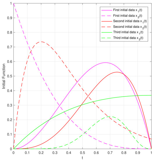
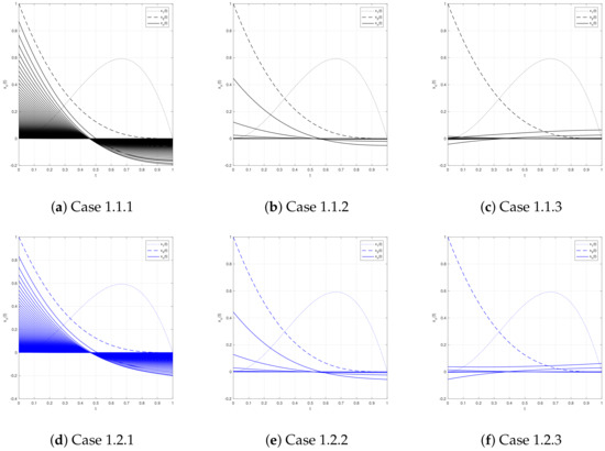
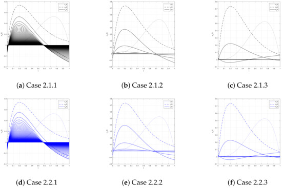
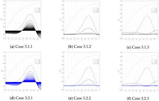
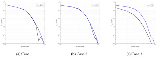
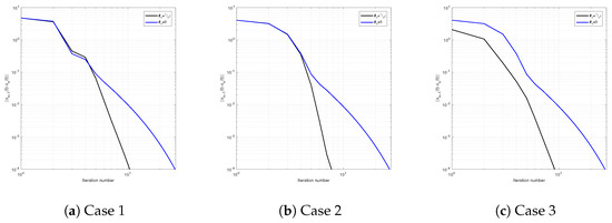
In this experiment, the stopping criterion is Cauchy error $\parallel x_{n+1}-x_n\parallel <{10}^{-4}$. The initial functions for each case are depicted in Figure 1. Figure 2, Figure 3 and Figure 4 illustrate the convergence behaviors of sequence $\left\{x_n\left(t\right)\right\}$ with and without the extrapolation factor $\left({\theta }_n\right)$ for Cases 1–3. Cauchy error plots for sequence $\left\{x_n\left(t\right)\right\}$ with and without extrapolation factor $\left({\theta }_n\right)$ are shown in Figure 5, Figure 6 and Figure 7 for ${\varrho }_n=0.1,2$, and $3.99$, respectively. Additionally, we demonstrate our algorithm’s performance in terms of iteration counts and CPU time for generating sequence $\left\{x_n\left(t\right)\right\}$ in each case, as shown in Table 1.

Figure 1. The initial functions $x_1$ and $x_2$ for each case in Example 1.

Figure 2. Convergence behavior of the sequence $\left\{x_n\left(t\right)\right\}$ with and without the extrapolation factor $\left({\theta }_n\right)$ for Case 1.

Figure 3. Convergence behavior of the sequence $\left\{x_n\left(t\right)\right\}$ with and without the extrapolation factor $\left({\theta }_n\right)$ for Case 2.

Figure 4. Convergence behavior of the sequence $\left\{x_n\left(t\right)\right\}$ with and without the extrapolation factor $\left({\theta }_n\right)$ for Case 3.

Figure 5. Cauchy error plots for the sequence $\left\{x_n\left(t\right)\right\}$ with and without the extrapolation factor $\left({\theta }_n\right)$ when ${\varrho }_n=0.1$.

Figure 6. Cauchy error plots for the sequence $\left\{x_n\left(t\right)\right\}$ with and without the extrapolation factor $\left({\theta }_n\right)$ when ${\varrho }_n=2$.

Figure 7. Cauchy error plots for the sequence $\left\{x_n\left(t\right)\right\}$ with and without the extrapolation factor $\left({\theta }_n\right)$ when ${\varrho }_n=3.99$.

Table 1. Comparison of iteration counts and CPU times for the sequence $\left\{x_n\left(t\right)\right\}$ of Example 1 in each case.

Cases	${\mathit{\varrho }}_{\mathit{n}}=0.1$				${\mathit{\varrho }}_{\mathit{n}}=2$				${\mathit{\varrho }}_{\mathit{n}}=3.99$
	${\theta }_n=\frac{1}{n^2}$		${\theta }_n=0$		${\theta }_n=\frac{1}{n^2}$		${\theta }_n=0$		${\theta }_n=\frac{1}{n^2}$		${\theta }_n=0$
	Iter.No.	CPU.Time (s)	Iter.No.	CPU.Time (s)	Iter.No.	CPU.Time (s)	Iter.No.	CPU.Time (s)	Iter.No.	CPU.Time (s)	Iter.No.	CPU.Time (s)
Case 1	151	30.1342	161	31.4323	9	4.3982	10	4.4201	11	4.6591	28	8.9243
Case 2	150	30.0023	160	31.1148	10	4.4520	11	4.4982	8	4.3988	28	8.9564
Case 3	124	26.1125	150	29.8753	9	4.3318	11	4.4885	10	4.5302	28	8.7685

Remark 1.

1. 

As illustrated in Figure 2, Figure 3 and Figure 4, the convergence behavior of sequence $\left\{x_n\left(t\right)\right\}$ generated by our proposed algorithm is observable. It always converges to zero, regardless of the initial and different parameters chosen.

2. 

Figure 5, Figure 6 and Figure 7 illustrated the Cauchy error generated by our proposed algorithm for sequence $\left\{x_n\left(t\right)\right\}$. It demonstrated that regardless of the parameters chosen, the algorithm with extrapolation factor $\left({\theta }_n\right)$ has a higher rate of convergence than the algorithm without it.

3. 

The advantages of our proposed algorithm in terms of iteration counts and CPU times are shown in Table 1. It demonstrated that the algorithm incorporating the extrapolation factor $\left({\theta }_n\right)$ is more efficient than the algorithm avoiding it.

Example 2.

Consider the following linear inverse problem: $y=Ax+b$, where $x\in {\mathbb{R}}^N$ is the signal to recover, $b\in {\mathbb{R}}^M$ is a noise vector, and $A:{\mathbb{R}}^N\to {\mathbb{R}}^M(M<N)$ is the acquisition device. To solve this inverse problem, we can convert it to the LASSO problem described below:

$$\begin{array}{c}\hfill \underset{x\in {\mathbb{R}}^N}{min}\frac{1}{2}{\parallel y-Ax\parallel }_2^2\mathit{subject}\mathit{to}{\parallel x\parallel }_1<r,\end{array}$$

(44)

where r is a positive constant. Assume that $C=\{z\in {\mathbb{R}}^N|\parallel z{\parallel }_1<q\}$ and that $Q=\left\{b\right\}$. The LASSO (44) problem then transforms into the spilt feasibility problem (1). Thus, as described in Corollary 1, Algorithm 2 can be used to recover a sparse signal $x\in {\mathbb{R}}^N$ with $k(k\ll N)$ nonzero elements.

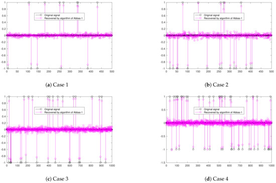
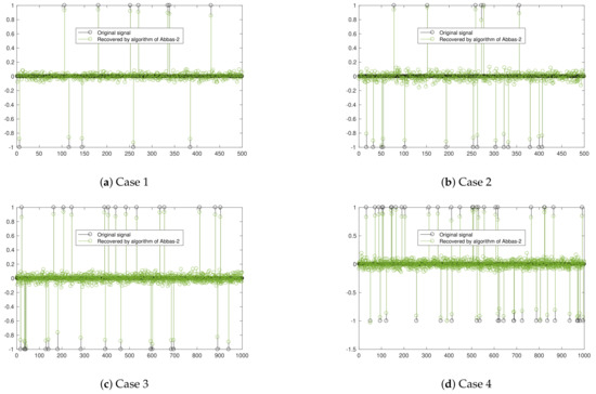
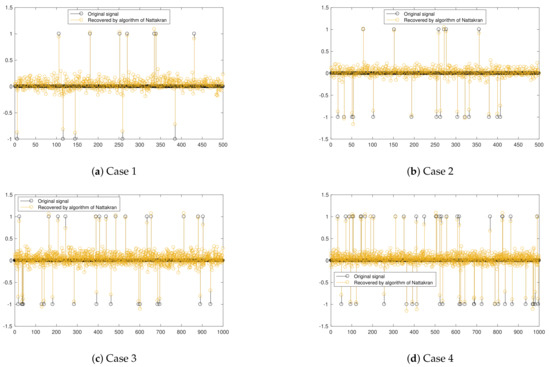
The purpose of this experiment is to demonstrate that Algorithm 2 can be used to solve the LASSO problem (44). Following that, we compare our algorithm to two strong convergence algorithms proposed by Abbas and Alshahrani [31]. These algorithms are referred to as Abbas-1 (17) and Abbas-2 (18), respectively. Additionally, we compare the algorithms to Kaewyong’s self-adaptive step size algorithm [32]. Nattakarn (19) is the name given to this algorithm.

Throughout all algorithms, we set regularization parameter $\lambda =1$ and ${\varrho }_n=2$. In our algorithm, we set $a_n=\frac{1}{n+1},b_n=\frac{1}{{(2n+1)}^2}$, $D\equiv F\equiv I$, $\xi =1$, $\alpha =1$, and ${\theta }_n=\frac{1}{n^2}$. In Nattakarn (19), we set $S\equiv I$, ${\alpha }_n=0.25$, ${\delta }_n=\frac{1}{n+1}$, $v=0.5$, and ${\theta }_n=\frac{1}{n^2}$. In Abbas-1 (17) and Abbas-2 (18), we set ${ϵ}_n=\frac{1}{n+1}$.

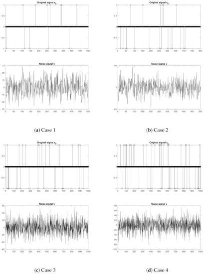
We evaluated the computational performance of each algorithm in a variety of different dimensions N and sparsity levels k (Case 1: $N=500,k=12$; Case 2: $N=500,k=20$; Case 3: $N=1000,k=30$; Case 4: $N=1000,k=50$). The number of iterations 200 is a used criterion for stopping. Additionally, we use the signal-to-noise ratio $SNR=20log\frac{\parallel x_0{\parallel }_2}{\parallel x_0-{x_{n+1}\parallel }_2}$, where $x_0$ is an original signal, to quantify the quality of recovery, with a higher SNR indicating a higher-quality recovery.

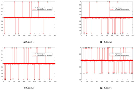
Figure 8 illustrates the original and noise signals in various dimensions N and sparsities k. Figure 9, Figure 10, Figure 11 and Figure 12 illustrate the recovery performance of all algorithms in a variety of scenarios. Table 2 shows the SNR comparison results.

Figure 8. Original and noise signals in various dimentions N and sparsities k in Example 2.

Figure 9. Recovery result by using Algorithm 2 in Example 2.

Figure 10. Recovery result by using Abbas-1 (17) in Example 2.

Figure 11. Recovery result by using algorithm Abbas-2 (18) in Example 2.

Figure 12. Recovery result by using Nattakran (19) in Example 2.

Table 2. SNR comparison results between Algorithm 2, Abbas-1 (17), Abbas-2 (18), and Nattakran (19).

Cases	N	k	Algorithm 2	Abbas-1 (17)	Abbas-2 (18)	Nattakran (19)
Case 1	500	12	43.1603	11.4874	11.5084	9.2145
Case 2	500	20	42.6409	14.3631	14.6021	12.4844
Case 3	1000	30	42.4700	14.3620	14.5633	10.4168
Case 4	1000	50	42.4067	12.9191	12.9341	12.4989

Remark 2.

1. 

As demonstrated in Example 2, our proposed algorithm is capable of solving the LASSO problem (44).

2. 

As showed in Table 2, Figure 9, Figure 10, Figure 11 and Figure 12, our algorithm outperforms other algorithms for solving the LASSO problem (44). Additionally, the dimensions and sparsities have no effect on computational performance of our proposed algorithm.

5. Conclusions

In this work, the split minimization problem was described in the framework of Hilbert spaces. By studying the advantages and disadvantages of some of the previous works, in this work, we constructed new algorithms for solving the split minimization problem by developing previously published algorithms based on useful techniques. The algorithms we constructed were combined with the following techniques: (1) self-adaptive step size technique to avoid computing the operator norm of a bounded linear operator norm, which is difficult if not impossible to calculate or even estimate, and (2) inertia and conjugate gradient direction techniques to speed up the convergence rate. In part of the numerical examples, we showed that the extrapolation factor $\left({\theta }_n\right)$ in the inertia term results in a faster rate of convergence and that the step size parameter affects the rate of convergence as well. Additionally, we applied our proposed algorithm to solve the signal recovery problem. We compared our algorithm’s recovery signal quality performance to that of three previously published works, which showed that our proposed algorithm outperformed other algorithms for solving the signal recovery problem.

References

- Censor, Y.; Elfving, T. A multiprojection algorithm using Bregman projections in a product space. Numer. Algorithms 1994, 8, 221–239. [Google Scholar] [CrossRef]
- Shi, Z.; Zhou, C.; Gu, Y.; Goodman, N.A.; Qu, F. Source estimation using coprime array: A sparse reconstruction perspective. IEEE Sens. J. 2016, 17, 755–765. [Google Scholar] [CrossRef]
- Zhou, C.; Gu, Y.; Zhang, Y.D.; Shi, Z.; Jin, T.; Wu, X. Compressive sensing-based coprime array direction-of-arrival estimation. IET Commun. 2017, 11, 1719–1724. [Google Scholar] [CrossRef]
- Zheng, H.; Shi, Z.; Zhou, C.; Haardt, M.; Chen, J. Coupled coarray tensor CPD for DOA estimation with coprime L-shaped array. IEEE Signal Process. Lett. 2021, 28, 1545–1549. [Google Scholar] [CrossRef]
- Byrne, C. Iterative oblique projection onto convex sets and the split feasibility problem. Inverse Probl. 2002, 18, 441. [Google Scholar] [CrossRef]
- Ansari, Q.H.; Rehan, A. Split feasibility and fixed point problems. In Nonlinear Analysis; Springer: Heidelberg, Germany, 2014; pp. 281–322. [Google Scholar]
- Boikanyo, O.A. A strongly convergent algorithm for the split common fixed point problem. Appl. Math. Comput. 2015, 265, 844–853. [Google Scholar] [CrossRef]
- Ceng, L.C.; Ansari, Q.; Yao, J.C. Relaxed extragradient methods for finding minimum-norm solutions of the split feasibility problem. Nonlinear Anal. Theory Methods Appl. 2012, 75, 2116–2125. [Google Scholar] [CrossRef]
- Moudafi, A.; Thakur, B. Solving proximal split feasibility problems without prior knowledge of operator norms. Optim. Lett. 2014, 8, 2099–2110. [Google Scholar] [CrossRef] [Green Version]
- Shehu, Y.; Cai, G.; Iyiola, O.S. Iterative approximation of solutions for proximal split feasibility problems. Fixed Point Theory Appl. 2015, 2015, 1–18. [Google Scholar] [CrossRef] [Green Version]
- Shehu, Y.; Iyiola, O.S.; Enyi, C.D. An iterative algorithm for solving split feasibility problems and fixed point problems in Banach spaces. Numer. Algorithms 2016, 72, 835–864. [Google Scholar] [CrossRef]
- Shehu, Y.; Ogbuisi, F.; Iyiola, O. Convergence analysis of an iterative algorithm for fixed point problems and split feasibility problems in certain Banach spaces. Optimization 2016, 65, 299–323. [Google Scholar] [CrossRef]
- Xu, H.K. Iterative methods for the split feasibility problem in infinite-dimensional Hilbert spaces. Inverse Probl. 2010, 26, 105018. [Google Scholar] [CrossRef]
- Yang, Q. On variable-step relaxed projection algorithm for variational inequalities. J. Math. Anal. Appl. 2005, 302, 166–179. [Google Scholar] [CrossRef] [Green Version]
- Gibali, A.; Mai, D.T. A new relaxed CQ algorithm for solving split feasibility problems in Hilbert spaces and its applications. J. Ind. Manag. Optim. 2019, 15, 963. [Google Scholar] [CrossRef] [Green Version]
- Moudafi, A.; Gibali, A. l 1-l 2 regularization of split feasibility problems. Numer. Algorithms 2018, 78, 739–757. [Google Scholar] [CrossRef] [Green Version]
- Shehu, Y.; Iyiola, O.S. Convergence analysis for the proximal split feasibility problem using an inertial extrapolation term method. J. Fixed Point Theory Appl. 2017, 19, 2483–2510. [Google Scholar] [CrossRef]
- López, G.; Martín-Márquez, V.; Wang, F.; Xu, H.K. Solving the split feasibility problem without prior knowledge of matrix norms. Inverse Probl. 2012, 28, 085004. [Google Scholar] [CrossRef]
- Zeidler, E. Nonlinear Functional Analysis and Its Applications: III: Variational Methods and Optimization; Springer Science & Business Media: New York, NY, USA, 2013. [Google Scholar]
- Nocedal, J.; Wright, S. Numerical Optimization; Springer Science & Business Media: New York, NY, USA, 2006. [Google Scholar]
- Sakurai, K.; Iiduka, H. Acceleration of the Halpern algorithm to search for a fixed point of a nonexpansive mapping. Fixed Point Theory Appl. 2014, 2014, 1–11. [Google Scholar] [CrossRef] [Green Version]
- Polyak, B.T. Some methods of speeding up the convergence of iteration methods. Ussr Comput. Math. Math. Phys. 1964, 4, 1–17. [Google Scholar] [CrossRef]
- Nesterov, Y. A method of solving a convex programming problem with convergence rate O (1/k2) O (1/k2). Sov. Math. Dokl 1983, 27, 372–376. [Google Scholar]
- Dang, Y.; Sun, J.; Xu, H. Inertial accelerated algorithms for solving a split feasibility problem. J. Ind. Manag. Optim. 2017, 13, 1383–1394. [Google Scholar] [CrossRef] [Green Version]
- Lorenz, D.A.; Pock, T. An inertial forward-backward algorithm for monotone inclusions. J. Math. Imaging Vis. 2015, 51, 311–325. [Google Scholar] [CrossRef] [Green Version]
- Kitkuan, D.; Kumam, P.; Martínez-Moreno, J.; Sitthithakerngkiet, K. Inertial viscosity forward–backward splitting algorithm for monotone inclusions and its application to image restoration problems. Int. J. Comput. Math. 2020, 97, 482–497. [Google Scholar] [CrossRef]
- Ul Rahman, J.; Chen, Q.; Yang, Z. Additive Parameter for Deep Face Recognition. Commun. Math. Stat. 2020, 8, 203–217. [Google Scholar] [CrossRef]
- Jyothi, R.; Babu, P. TELET: A Monotonic Algorithm to Design Large Dimensional Equiangular Tight Frames for Applications in Compressed Sensing. arXiv 2021, arXiv:2110.12182. [Google Scholar] [CrossRef]
- Rockafellar, R.T.; Wets, R.J.B. Variational Analysis; Springer Science & Business Media: New York, NY, USA, 2009; Volume 317. [Google Scholar]
- Aubin, J.P. Optima and Equilibria: An Introduction to Nonlinear Analysis; Springer Science & Business Media: New York, NY, USA, 2013; Volume 140. [Google Scholar]
- Abbas, M.; AlShahrani, M.; Ansari, Q.H.; Iyiola, O.S.; Shehu, Y. Iterative methods for solving proximal split minimization problems. Numer. Algorithms 2018, 78, 193–215. [Google Scholar] [CrossRef]
- Kaewyong, N.; Sitthithakerngkiet, K. A Self-Adaptive Algorithm for the Common Solution of the Split Minimization Problem and the Fixed Point Problem. Axioms 2021, 10, 109. [Google Scholar] [CrossRef]
- Moreau, J.J. Propriétés des applications «prox». Comptes Rendus Hebdomadaires des Séances de l’Académie des Sci. 1963, 256, 1069–1071. [Google Scholar]
- Moreau, J.J. Proximité et dualité dans un espace hilbertien. Bull. de la Société Mathématique de Fr. 1965, 93, 273–299. [Google Scholar] [CrossRef]
- Combettes, P.L.; Wajs, V.R. Signal recovery by proximal forward-backward splitting. Multiscale Model. Simul. 2005, 4, 1168–1200. [Google Scholar] [CrossRef] [Green Version]
- Micchelli, C.A.; Shen, L.; Xu, Y. Proximity algorithms for image models: Denoising. Inverse Probl. 2011, 27, 045009. [Google Scholar] [CrossRef]
- Bauschke, H.H.; Combettes, P.L. Convex Analysis and Monotone Operator Theory in Hilbert Spaces; Springer: Berlin, Germany, 2011; Volume 408. [Google Scholar]
- Xu, H.K. Iterative algorithms for nonlinear operators. J. Lond. Math. Soc. 2002, 66, 240–256. [Google Scholar] [CrossRef]
- Maingé, P.E. Strong convergence of projected subgradient methods for nonsmooth and nonstrictly convex minimization. Set-Valued Anal. 2008, 16, 899–912. [Google Scholar] [CrossRef]
Publisher’s Note: MDPI stays neutral with regard to jurisdictional claims in published maps and institutional affiliations. |
© 2022 by the authors. Licensee MDPI, Basel, Switzerland. This article is an open access article distributed under the terms and conditions of the Creative Commons Attribution (CC BY) license (https://creativecommons.org/licenses/by/4.0/).