Bayesian and Non-Bayesian Estimation of the Nadaraj ah–Haghighi Distribution: Using Progressive Type-1 Censoring Scheme

Abstract

This work will address the problem of estimating the parameters for the Nadaraj ah–Haghighi (NH) distribution using progressive Type-1 censoring (PT1C) utilizing Bayesian and non-Bayesian approaches. To apply PT1C, censoring times for each stage of censoring needed to be known before the experiment started. To solve this issue of censoring time selection, qauntiles from the NH lifetime distribution will be used as PT1C censoring time points. Maximum likelihood (ML) estimators (MLEs) and asymptotic confidence intervals (ACoIs) are produced with a focus on the censoring technique. Bayes estimates (BEs) and accompanying maximum posterior density (PD) credible interval estimations are also created via the squared error (SEr) loss function. The BEs are evaluated using the Markov Chain Monte Carlo (MCMC) technique and the Metropolis–Hasting (MH) algorithm. An analysis of an actual data set demonstrates the theoretical implications of MLEs and BEs for defined schemes of PT1C samples. Finally, simulation results will be used to compare the performance of the various recommended estimators.

1. Introduction

Expanding continuous univariate distributions through adding a few more shape parameters is an important way of better exploring the skewness and tail weights, as well as other features of the produced distributions. Due to the recent trend, applied statisticians may now create more extended distributions that yield superior goodness-of-fit metrics whenever fitted to real data rather than just the classical distributions. The exponential (Ex) model is likely the most commonly used statistical distribution for analysis of survival and reliability concerns. The above model was the earliest in the lifetime literature about which statistical methods became substantially explored. Ref. [1] recently presented a generalization of the Ex distribution known as the Nadaraj ah–Haghighi (NH) distribution. Both distribution function (cdf) and probability density function (pdf) are computed on the basis of

$$G\left(z\right)=1-\exp \left[1-{\left(1+\lambda z\right)}^{\alpha }\right],z>0,$$

(1)

and

$$g\left(z\right)=\alpha \lambda {\left(1+\lambda z\right)}^{\alpha -1}\exp \left[1-{\left(1+\lambda z\right)}^{\alpha }\right],z>0,\alpha ,\lambda >0.$$

(2)

The quantile function (quf) of random variable (R-V) Z are

$$z=\frac{1}{\lambda }\left(\sqrt[\alpha ]{1-ln\left(1-u\right)}-1\right).$$

(3)

In terms of fitting real-life data, the NH distribution is a fairly flexible lifespan model. The NH distribution, like the standard Weibull distribution, gamma distribution, or modified exponential distribution, may simulate decreasing, increasing, or constant hazard rates. Furthermore, this model is a subset of the generalized power Weibull distribution, which was presented in [2]. In the literature, the NH distribution has attracted a great attention and has already been researched by a lot of scientists. Consider, for instance, [3,4] works. Furthermore, the NH distribution is also known as the extended Ex distribution in certain other publications, which including [5,6]. Ref. [1] discovered that even if certain data sets had the number zero, an NH model may still produce adequate fits. Furthermore, under this distribution, the trend of the hazard rate function (hrf) is sensitive on $\alpha$. For example, when $\alpha >1(\alpha <1)$, the hrf tends to grow (reduce). However, when $\alpha$ is set to 1, the hrf becomes a constant. At this point, (1) also becomes the Ex distribution.

There is some material available about estimation of the NH distribution. Regarding the estimate of unknown parameters, Ref. [7] has studied the maximum likelihood (ML) and Bayes estimations using progressive type-2 censored (PT2C) samples with binomial removals. Subsequently, Ref. [8] looked at PT2C data. They computed MLEs using the Newton–Raphson technique and BEs using the MCMC methodology. Asymptotic confidence intervals (ACoIs) and highest PD (HPD) intervals were also estimated. Several sources, such as [5,6], also focused on the issues of order statistics (OS) of an NH distribution. They jointly developed on moment recurrence formulations for OS. The former, on the other hand, dealt with the problem in PT2C, whilst the latter concentrated on the entire sample set. In addition, Ref. [9] explored MLEs and BEs using the Lindley approximation for the unknown parameters. Non-Bayesian and Bayesian predictions were also used to make point and interval forecasts for future data. Furthermore, Ref. [10] investigated the MLEs and BEs for the two unknown parameters and lifespan parameters of survival and hrfs using the gradually first-failure censored NH model. They also proposed an optimum filtering strategy based on several optimality criteria. The MLEs and BEs for the constant stress partly accelerated life tests under PT2C were explored in ref. [11]. The estimate and prediction of the NH distribution under PT2C were addressed in ref. [12].

Censored data occurs in real-world testing trials when studies, including the lifespan of test units, must be ended before complete observation. Censoring is a typical and inevitable practice action for a variety of reasons, including time constraints and cost savings. Censorship of various forms has been thoroughly investigated, with Type-1 and Type-2 censorship being the most common. In comparison to traditional censorship designs, a generalized style of censorship known as PC schemes has lately received significant attention in the works due to its effective use of available resources. One of these PC schemes is PT1C. This trend is observed when a specific number of lifespan test units are consistently excluded from the test at the end of each post-test period of time. The capacity to determine the termination time realistically and additional design freedom by allowing test units to be terminated during non-terminal time periods [13]. Bayesian and classical inference for odd Lindley Burr XII model are proposed in [14] and Topp-Leone NH distribution are proposed in [15].

Assume a life testing experiment has n units. Presume that $Z_1,Z_2,\dots ,Z_n$ represent the lifetime of all n units taken from a population. Suppose that $z_{\left(1\right)}<z_{\left(2\right)}<\dots <z_{\left(n\right)}$ denotes the respective ordered lifespan recorded from the life test. At the end of the preset period of censoring $Tqi$, $Ri$ items are excluded from the surviving items in accordance with $q{i}^{th}$ Qs, $i=1,2,\dots ,m$, where m signifies the number of testing phase, $T_{q_i}>T_{q_{i-1}}$ and $n=r+{\sum }_{i=1}^m{R}_i$.

The quantities $T_{q_i}$ should always be determined ahead of time:

• Predicated on the experimenter’s past knowledge and skills with the objects under consideration [16], or
• The Qs of the lifetimes distribution, $qi$th, which possibly calculated by using the provided expression

$$P(Z\le T_{q_i})=q_i\Rightarrow T_{q_i}=F^{-1}\left(q_i\right)i=1,2,\dots ,m.$$

Within those cases, $Ri,Tqi$ and n are fixed and constant, whereas $li$ represents the quantity of surviving entities at a particular moment in time, and $Tqi$ and $r=\sum {i=1}^{m}li$ are R-Vs. The likelihood (L-L) function is represented as

$$\ell \left(\theta \right)\propto \prod _{i=1}^{r}f(z_{\left(i\right)};\theta )\prod _{k=1}^s{\left(1-F(T_{\left(q_k\right)};\theta )\right)}^{R_k}$$

(4)

wherein $z\left(i\right)$ is the observable lifespan of the ith OS [17]. This censorship mechanism is depicted in Figure 1 see [18].

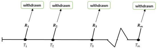
Figure 1. PT1C Scheme.

Complete samples, as well as the Type-1 censoring scheme, can indeed be viewed as special examples of this censoring technique.

The PT1C technique for the Weibull distribution was introduced in reference [17]. The MLEs and BEs for the unknown parameters of the generalized inverse Ex distribution under PT1C were obtained in [19]. For the PT1C, there are two publications that are closely linked. The first was the MLEs and ACI estimates for the parameters of the extended inverse Ex model, predicated on the premise that there are two kinds of failures [20]. The second were the MLEs and BEs for the unknown parameters of the extended inverse Ex model [21]. Ref. [22] investigates the statistical inference of the inverse Weibull model under PT1C.

The goal of this work is to examine the PT1C scheme where each lifetime has its own NH model. We employ two independent approaches to drive the MLEs and BEs, and then use MCMC to calculate the ACI of these various parameters. We examine simulation results as well as actual data sets to evaluate how the various models work in practice. The next thing is how the entire article is structured: the second The section discusses the MLE and confidence intervals. The Metropolis–Hasting (MH) method is utilized in the third section to investigate the Bayesian estimation approach, which completely certifies the gamma model as a prior distribution for unknown parameters. The fourth section uses simulated results and a real data set to show the theoretical findings. Finally, there are some closing remarks and a summary.

2. Maximum Likelihood Approach

This section examines the MLE estimation strategy based on the PT1C strategy for the unknown parameters of the NH distribution. It is how the PT1C approach is suitable:

• In a real-world experiment, test a random sample of n units with the next lifespan NH($\alpha$,$\lambda$) model.
• Prefix s censoring time points $T_{q_1},\dots ,T_{q_s}$, at which fixed quantity $R_1,\dots ,\dots ,R_{s-1}$ of surviving items are eliminated from the test at randomized. The censoring times $T_{q_k}$ are chosen equivalent to $P(Z\le T_{q_k})=q_k$, where Z∼ NH($\alpha$,$\lambda$) and $q_k^{th}$ is the Qs ($k=1,2,\dots ,s$) in terms of the desired lifetime distribution.
• The life test ends at just before a predetermined time $T_{q_s}$.

As a result, using the same censoring process, one may generate PT1C samples $\mathbf{z}=(z_{\left(1\right)},z_{\left(2\right)},\dots ,z_{\left(r\right)})$ indicating the reported lifetime of r units.

Using (2) of NH model in (4) of L-L function under PT1C, the linked L-L function of $\alpha$ and $\lambda$ given the PT1C data, $\mathbf{z}$, might be regarded as

$$\ell \left(\alpha ,\lambda \right)\propto {\left(\alpha \lambda \right)}^r\prod _{i=1}^r{\left(1+\lambda z_i\right)}^{\alpha -1}\prod _{i=1}^r\exp \left[1-{\left(1+\lambda z_i\right)}^{\alpha }\right]\prod _{k=1}^s{\left(1-\exp \left[1-{\left(1+\lambda T_{q_k}\right)}^{\alpha }\right]\right)}^{R_k}.$$

(5)

By taking the logarithm function of L-L to obtain log-L-L ($\mathcal{L}$) as

$$\mathcal{L}\propto rln\alpha +rln\lambda +\left(\alpha -1\right)\sum _{i=1}^{r}ln\left(1+\lambda z_i\right)+\sum _{i=1}^r\left[1-{\left(1+\lambda z_i\right)}^{\alpha }\right]+\sum _{k=1}^s{R_{k}ln\left(1-A_k\right)}^{\alpha }.$$

First partial derivatives of $\mathcal{L}$ in regard to $\alpha$ and $\lambda$ are calculated in the following manner:

$$\begin{array}{cc}\hfill \frac{\partial \mathcal{L}}{\partial \alpha }& =\frac{r}{\alpha }+\sum _{i=1}^{r}ln\left(1+\lambda z_i\right)-\sum _{i=1}^r{\left(1+\lambda z_i\right)}^{\alpha }ln(1+\lambda z_i)+\sum _{k=1}^s\frac{R_k{A}_k{B}_{k}ln\left(C_k\right)}{1-A_k},\hfill \end{array}$$

(6)

and

$$\begin{array}{cc}\hfill \frac{\partial \mathcal{L}}{\partial \lambda }& =\frac{r}{\lambda }+\left(\alpha -1\right)\sum _{i=1}^r\frac{z_i}{1+\lambda z_i}-\alpha z_i\sum _{i=1}^r{\left(1+\lambda z_i\right)}^{\alpha -1}+\sum _{k=1}^s\frac{\alpha R_k{A}_k{C_k}^{\alpha -1}{T}_{q_k}}{1-A_k},\hfill \end{array}$$

(7)

where $A_k=\exp [1-B_k]$, $B_k={C_k}^{\alpha }\left]\right)$ and $C_k=\left(1+\lambda T_{q_k}\right)$.

Equating $\frac{\partial \mathcal{L}}{\partial \alpha }{|}_{\alpha =\widehat{\alpha }}$ and $\frac{\partial \mathcal{L}}{\partial \lambda }{|}_{\lambda =\widehat{\lambda }}$ to 0, The MLEs of $\alpha$ and $\lambda$ are the empirical solutions of the preceding two equations for $\widehat{\alpha }$ and $\widehat{\lambda }$.

3. Bayesian Estimation

In this part, we will look at how to use Bayesian estimation to estimate the parameters of an NH model using the PT1C method. The standard error (SEr) loss function will be used for Bayesian estimation. It is feasible to employ distinct gamma priors for the NH model parameters $\alpha$ and $\lambda$ with pdfs

$$\begin{array}{cc}\hfill {\pi }_1\left(\alpha \right)& \propto {\alpha }^{a-1}exp(-b\alpha ),\alpha >0,a>0,b>0,\hfill \end{array}$$

and

$$\begin{array}{cc}\hfill {\pi }_2\left(\lambda \right)& \propto {\lambda }^{c-1}exp(-d\lambda ),\lambda >0,c>0,d>0.\hfill \end{array}$$

Pursuant to the data compiled, the appropriate PD $\mathbf{z}=(z_{\left(1\right)},z_{\left(2\right)},\dots ,z_{\left(r\right)})$ could be represented in fact as

$$\pi (\alpha ,\lambda |\mathbf{z})=\frac{\pi (\alpha ,\lambda )L(\alpha ,\lambda )}{{\int }_0^{\infty }{\int }_0^{\infty }\pi (\alpha ,\lambda )L(\alpha ,\lambda )d\alpha d\lambda }$$

The PD function has been written in the form

$$\begin{array}{cc}\hfill \pi (\alpha ,\lambda |\mathbf{z})& =K^{-1}[{\alpha }^{r+a-1}{\lambda }^{r+c-1}exp\left(-b\alpha -d\lambda \right)\prod _{i=1}^r{\left(1+\lambda z_i\right)}^{\alpha -1}\hfill \\ \hfill & \prod _{i=1}^r{\exp [1-\left(1+\lambda z_i\right)}^{\alpha }]\prod _{k=1}^s{\left(1-\exp \left[1-{\left(1+\lambda T_{q_k}\right)}^{\alpha }\right]\right)}^{R_k}],\hfill \end{array}$$

where

$$\begin{array}{cc}\hfill K& ={\int }_0^{\infty }{\int }_0^{\infty }[{\alpha }^{r+a-1}{\lambda }^{r+c-1}exp\left(-b\alpha -d\lambda \right)\prod _{i=1}^r{\left(1+\lambda z_i\right)}^{\alpha -1}\hfill \\ \hfill & \prod _{i=1}^r{\exp [1-\left(1+\lambda z_i\right)}^{\alpha }]\prod _{k=1}^s{\left(1-\exp \left[1-{\left(1+\lambda T_{q_k}\right)}^{\alpha }\right]\right)}^{R_k}]d\alpha d\lambda .\hfill \end{array}$$

As just an outcome, the PD could be changed as tries to follow:

$$\begin{array}{cc}\hfill \pi (\alpha ,\lambda |\mathbf{z})& \propto [{\alpha }^{r+a-1}{\lambda }^{r+c-1}exp\left(-b\alpha -d\lambda \right)\prod _{i=1}^r{\left(1+\lambda z_i\right)}^{\alpha -1}\hfill \end{array}$$

(8)

$$\begin{array}{cc}\hfill & \prod _{i=1}^r{\exp [1-\left(1+\lambda z_i\right)}^{\alpha }]\prod _{k=1}^s{\left(1-\exp \left[1-{\left(1+\lambda T_{q_k}\right)}^{\alpha }\right]\right)}^{R_k}].\hfill \end{array}$$

(9)

The Bayes estimator about any function, such like $g(\alpha ,\lambda )$, is supplied by the SEr

$$\tilde{g}(\alpha ,\lambda )={\int }_0^{\infty }{\int }_0^{\infty }g(\alpha ,\lambda )\pi (\alpha ,\lambda |x)d\alpha d\lambda .$$

(10)

As a result, Equation (10) cannot be computed for generic $g(\alpha ,\lambda )$. As an outcome, we propose that you employ the most often used estimated BEs of $\alpha$ and $\lambda$ MCMC.

3.1. Metropolis–Hasting Algorithm

To perform the MH method for the NH distribution, we must supply the NH model and initial values for the unknown parameters $\alpha$ and $\lambda$. For the suggestion model, we investigate a bivariate normal distribution, that is $q\left(({\alpha }^{{}^{\prime }},{\lambda }^{{}^{\prime }})|(\alpha ,\lambda )\right)\equiv N_2((\alpha ,\lambda ),S_{\alpha ,\lambda })$, We might receive unfavorable feedback, which really is undesired, if $S\alpha ,\lambda$ describes the variance-covariance matrix. To establish the initial values, we apply the MLE for $\alpha$ and $\lambda$, that is $({\alpha }^{\left(0\right)},{\lambda }^{\left(0\right)})=(\hat{\alpha },\hat{\lambda })$. The MH technique uses the following stages to select a sample from the PD provided by Equation (10) are delivered in the prescribed sequence:

• Step I Set the initial magnitude of $\theta$ to ${\theta }^{\left(0\right)}=\left(\hat{\alpha },\hat{\lambda }\right)$.
• Step II For $i=1,2,\dots ,M$ the following phases must be reproduced:
  •  2.1: Set $\theta ={\theta }^{(i-1)}$.
  •  2.2: Make a new value for the contender parameter $\delta$ from $N_2\left(ln\theta ,S_{\theta }\right)$.
  •  2.3: Set ${\theta }^{{}^{\prime }}=exp\left(\delta \right)$.
  •  2.4: Compute $\beta =\frac{\pi \left({\theta }^{{}^{\prime }}\right|x)}{\pi \left({\theta }^{|}x\right)}$, where $\pi (·)$ is the PD.
  •  2.5: Create a sample u through using uniform $U(0,1)$ distribution.
  •  2.6: Accept or reject the specific request premised on ${\theta }^{{}^{\prime }}$

    $$\left\{\begin{array}{cc}\mathrm{If}u\le \beta \hfill & \mathrm{set}{\theta }^{\left(i\right)}={\theta }^{{}^{\prime }}\hfill \\ \mathrm{otherwise}\hfill & \mathrm{set}{\theta }^{\left(i\right)}=\theta .\hfill \end{array}\right.$$

Consequently, to use the PD’s random samples of size M, a portion of the original samples might well be removed (burn-in), and the remaining samples can really be utilized to generate BEs. The Equation (10) can really be approximated more exactly as

$${\tilde{g}}_{MH}(\gamma ,\lambda )=\frac{1}{M-l_B}\sum _{i=l_B}^{M}g({\alpha }_i,{\lambda }_i),$$

(11)

where $l_B$ is the overall amount of burn-in samples.

3.2. Highest Posterior Density (HDP)

We establish HPD intervals for the unknown parameters $\alpha$ and $\lambda$ of the NH distribution under PT1C using the samples obtained by the suggested MH approach in the preceding paragraph. Considering the next case study: ${\alpha }^{\left(\delta \right)}$ and ${\lambda }^{\left(\delta \right)}$ be the $\delta$th Q of $\alpha$ and $\lambda$, respectively, that is,

$$\left({\alpha }^{\left(\delta \right)},{\lambda }^{\left(\delta \right)}\right)=inf\{\left(\alpha ,\lambda \right):\Pi \left((\alpha ,\lambda )|\mathbf{z}\right)\ge \delta \},$$

where $0<\delta <1$ and $\Pi (·)$ is the PD of $\alpha$ and $\lambda$. It should be noted that for a given ${\alpha }^{*}$ and ${\lambda }^{*}$, an accurate estimator based on simulation of $\pi \left((\alpha ,\lambda )|\mathbf{z}\right)$ might well be computed as

$$\Pi \left(({\alpha }^{*},{\lambda }^{*})|\mathbf{z}\right)=\frac{1}{M-l_B}\sum _{i=l_B}^M{I}_{(\alpha ,\lambda )\le ({\alpha }^{*},{\lambda }^{*})}$$

Here $I_{(\alpha ,\lambda )\le ({\alpha }^{*},{\lambda }^{*})}$ is the indicator function. The proper estimate is then determined as

$$\hat{\Pi }\left(({\alpha }^{*},{\lambda }^{*})|\mathbf{z}\right)=\left\{\begin{array}{cc}0\hfill & \mathrm{if} ({\alpha }^{*},{\lambda }^{*})<({\alpha }_{\left(l_B\right)},{\lambda }_{\left(l_B\right)})\hfill \\ \sum _{j=l_B}^i{\omega }_j\hfill & \mathrm{if} ({\alpha }_{\left(i\right)},{\lambda }_{\left(i\right)})<({\alpha }^{*},{\lambda }^{*})<({\alpha }_{(i+1)},{\lambda }_{(i+1)})\hfill \\ 1\hfill & \mathrm{if} ({\alpha }^{*},{\lambda }^{*})>({\alpha }_{\left(M\right)},{\lambda }_{\left(M\right)})\hfill \end{array}\right.$$

where ${\omega }_j=\frac{1}{M-l_B}$ and $({\alpha }_{\left(j\right)},{\lambda }_{\left(j\right)})$ are the ordered values of $({\alpha }_j,{\lambda }_j)$. Now, for $i=l_B,\dots ,M$, $({\alpha }^{\left(\delta \right)},{\lambda }^{\left(\delta \right)})$ may be estimated by

$$\left({\tilde{\alpha }}^{\left(\delta \right)},{\tilde{\lambda }}^{\left(\delta \right)}\right)=\left\{\begin{array}{cc}({\alpha }_{\left(l_B\right)},{\lambda }_{(l-B)})\hfill & \mathrm{if}\delta =0\hfill \\ ({\alpha }_{\left(i\right)},{\lambda }_{\left(i\right)})\hfill & \mathrm{if} \sum _{j=l_B}^{i-1}{\omega }_j<\delta <\sum _{j=l_B}^i{\omega }_j.\hfill \end{array}\right.$$

Furthermore, let us determine a $100(1-\delta )\%$ HPD credible interval for $\alpha$ and $\lambda$

$$HP{D}_j^{\alpha }=({\tilde{\alpha }}^{\left(\frac{j}{M}\right)},{\tilde{\alpha }}^{\left(\frac{j+(1-\delta )M}{M}\right)})\&HP{D}_j^{\lambda }=\left({\tilde{\lambda }}^{\left(\frac{j}{M}\right)},{\tilde{\lambda }}^{\left(\frac{j+(1-\delta )M}{M}\right)}\right)$$

for $j=l_B,\dots ,\left[\delta M\right]$, here $\left[a\right]$ represents indicates the largest integer that $\le a$. Need to choose $HP{D}_{j^{*}}$ from one of many $HP{D}_j$’s with the narrowest width.

4. Numerical Outcomes

The purpose of this section is to compare the performance of the various estimating methods outlined in the previous sections. For illustrative purposes, we investigate a real data set; moreover, a simulation experiment is performed to test the statistical performances of the estimators under the PT1C scheme as well as the conduct of the recommended techniques. For calculations, we employed the R-statistical software.

4.1. Results of Simulation

Inside this section, we utilize computer simulations to test the efficiency of estimation methodologies, specifically MLE and Bayesian estimation, for something like the NH distribution using the PT1C scheme. We generate 1000 data points from the NH model with the standard procedures for such MLEs:

• $\alpha =0.5$ and $\lambda =1.5$, i.e., $NH(0.5,1.5)$.
• Sample sizes are $n=25$, $n=50$ and $n=100$.
• Number of stages of PT1C are $m=3,5$.
• Censoring times $T_j$ (CT) are discussed and recommendations:
  • $CT-I$ = (0.25, 0.55, 2)
  • $CT-II=(0.45,1.25,3.5)$
  • $CT-III=(0.15,0.45,0.85,1.5,2.6)$
  • $CT-IV=(0.30,0.70,1.25,2.13,4)$
  where $j=1,\dots ,m$. The patterns of CT can be classified according to m. In our study, $CT-I$ and $CT-II$ are used when $m=3$ and $CT-III$ and $CT-IV$ are used when $m=5$.
• Removed items $R_j$ are assumed at different sample size n as shown in Table 1 where $R_m=n-({\sum }_{j=1}^{m-1}{R}_j+r)$ and r is the number of failure items.
  Table 1. Numerous patterns for removing items from life test at numerous number of stages.

  m	Scheme	Patterns
  		$\mathbf{n}=\mathbf{25}$	$\mathbf{n}=\mathbf{50}$	$\mathbf{n}=\mathbf{100}$
  3	PT1C1	$\mathcal{R}=(0^{\left(2\right)},R_m)$	$\mathcal{R}=(0^{\left(2\right)},R_m)$	$\mathcal{R}=(0^{\left(2\right)},R_m)$
  	PT1C2	$\mathcal{R}=(3^{\left(2\right)},R_m)$	$\mathcal{R}=(5^{\left(2\right)},R_m)$	$\mathcal{R}=(9^{\left(2\right)},R_m)$
  	PT1C3	$\mathcal{R}=(5^{\left(2\right)},R_m)$	$\mathcal{R}=(9^{\left(2\right)},R_m)$	$\mathcal{R}=({18}^{\left(2\right)},R_m)$
  	PT1C4	$\mathcal{R}=(6,0,R_m)$	$\mathcal{R}=(10,0,R_m)$	$\mathcal{R}=(18,0,R_m)$
  	PT1C5	$\mathcal{R}=(10,0,R_m)$	$\mathcal{R}=(18,0,R_m)$	$\mathcal{R}=(36,0,R_m)$
  	PT1C6	$\mathcal{R}=(0,6,R_m)$	$\mathcal{R}=(0,10,R_m)$	$\mathcal{R}=(0,18,R_m)$
  	PT1C7	$\mathcal{R}=(0,10,R_m)$	$\mathcal{R}=(0,18,R_m)$	$\mathcal{R}=(0,36,R_m)$
  5	PTIC8	$\mathcal{R}=(0^{\left(4\right)},R_m)$	$\mathcal{R}=(0^{\left(4\right)},R_m)$	$\mathcal{R}=(0^{\left(4\right)},R_m)$
  	PT1C9	$\mathcal{R}=(2^{\left(4\right)},R_m)$	$\mathcal{R}=(3^{\left(4\right)},R_m)$	$\mathcal{R}=(5^{\left(4\right)},R_m)$
  	PT1C10	$\mathcal{R}=(3^{\left(4\right)},R_m)$	$\mathcal{R}=(5^{\left(4\right)},R_m)$	$\mathcal{R}=({10}^{\left(4\right)},R_m)$
  	PT1C11	$\mathcal{R}=(8,0^{\left(3\right)},R_m)$	$\mathcal{R}=(12,0^{\left(3\right)},R_m)$	$\mathcal{R}=(20,0^{\left(3\right)},R_m)$
  	PT1C12	$\mathcal{R}=(12,0^{\left(3\right)},R_m)$	$\mathcal{R}=(20,0^{\left(3\right)},R_m)$	$\mathcal{R}=(40,0^{\left(3\right)},R_m)$
  	PT1C13	$\mathcal{R}=(0^{\left(3\right)},8,R_m)$	$\mathcal{R}=(0^{\left(3\right)},12,R_m)$	$\mathcal{R}=(0^{\left(3\right)},20,R_m)$
  	PT1C14	$\mathcal{R}=(0^{\left(3\right)},12,R_m)$	$\mathcal{R}=(0^{\left(3\right)},20,R_m)$	$\mathcal{R}=(0^{\left(3\right)},40,R_m)$

  Here, (1⁽³⁾, 0), for example, means that the censoring scheme employed is (1, 1, 1, 0).

It is indicate that scheme PT1C1 and PT1C8 are represent Type-1 censoring scheme as a special case with number of failure items $R_m=n-r$ and CT is $T_m$. We compute MLEs and related 95% ACoI relying on the generated data. When calculating MLEs, the initial estimate values are assumed to be much like the genuine parameter values.

We compute BEs utilizing the MH algorithm with informative priors for the Bayesian estimation approach. As previous examples, we construct 1000 complete samples of size 60 from the $NH(0.5,2)$ model, and the hyper parameter values are $a=19.25, b=35.54,$$c=4.36, d=2.82$.

The aforementioned informative prior values are used to compute the required estimations. When using the MH approach, we use the MLEs as starting guess values, as well as the corresponding variance–covariance matrix $S_{\theta }$ of $(ln(\hat{\alpha }),ln(\hat{\lambda }))$. Subsequently, we removed 2000 burn-in samples from the total 10,000 samples generated by the PD, and then used the approach to derive BEs and HPD interval estimates of [23].

Table 2, Table 3 and Table 4 shows all of the average estimates including both approaches for samples size $n=25$, $n=50$, and $n=100$, respectively. Furthermore, the first row shows average estimations (Avg. ), whereas the second row reflects corresponding means square errors (MSErs). For CoIs, we have ACoI for MLEs and HPD for BEs premised on the MCMC results shown in Table 5, Table 6 and Table 7 for samples size $n=25$, $n=50$, and $n=100$, respectively. In addition, the first row indicates average interval lengths (AvILs), whereas the second row reflects corresponding coverage probabilities (CPrs).

Table 2. Average estimated values and MSErs of the ML and BEs for NH model with $\alpha =0.5$ and $\lambda =1.5$ under various censoring schemes at $n=25$.

m	Scheme		$\hat{\mathit{\alpha }}$	$\hat{\mathit{\lambda }}$	$\tilde{\mathit{\alpha }}$	$\tilde{\mathit{\lambda }}$	$\hat{\mathit{\alpha }}$	$\hat{\mathit{\lambda }}$	$\tilde{\mathit{\alpha }}$	$\tilde{\mathit{\lambda }}$
3			CT-I = (0.25, 0.55, 2)				CT-II = (0.45, 1.25, 3.5)
	PT1C1	Avg.	0.8948	2.6912	0.5501	1.3662	0.7484	2.0899	0.5249	1.3854
		MSE	2.2623	14.3597	0.2271	0.7710	1.0531	5.7098	0.0153	0.1591
	PT1C2	Avg.	1.0072	2.6698	0.5427	1.3888	0.8560	2.2173	0.5514	1.3967
		MSE	2.7397	16.9018	0.2662	1.5031	1.5397	7.9254	0.2437	1.8852
	PT1C3	Avg.	0.9250	3.4413	0.5305	1.3544	0.8516	2.6298	0.5331	1.3393
		MSE	2.9141	30.3084	0.0101	0.8317	1.7672	18.8783	0.2204	0.1812
	PT1C4	Avg.	1.0532	3.3816	0.5218	1.3179	1.0978	2.8243	0.5154	1.4354
		MSE	3.3939	34.4629	0.1262	0.2178	3.8031	20.8134	0.0188	3.1201
	PT1C5	Avg.	0.7825	6.2342	0.5751	1.3815	0.8827	3.6967	0.5307	1.3467
		MSE	2.1408	95.7135	0.6419	0.5359	1.9410	34.3576	0.3427	0.2143
	PT1C6	Avg.	0.9539	2.7382	0.5784	1.3628	0.7271	2.3022	0.5343	1.4304
		MSE	2.7866	15.4670	0.7044	0.1731	0.9632	8.0300	0.1255	1.2587
	PT1C7	Avg.	0.8849	2.4477	0.5432	1.4515	0.7408	2.0562	0.5585	1.2931
		MSE	1.9893	11.1132	0.1372	3.6322	0.7289	5.7175	0.2279	0.1638
5			CT-III = (0.15, 0.45, 0.85, 1.5, 2.6)				CT-IV = (0.30, 0.70, 1.25, 2.13, 4)
	PT1C8	Avg.	0.8481	2.1918	0.5349	1.4278	0.6786	1.9874	0.5373	1.4301
		MSE	1.7637	6.7086	0.1997	0.4305	0.3458	4.5281	0.1599	0.9719
	PT1C9	Avg.	0.8225	2.7283	0.5375	1.3397	0.9241	2.2212	0.5334	1.4292
		MSE	1.5673	14.4142	0.1224	0.5393	2.0320	9.2290	0.1605	0.4938
	PT1C10	Avg.	0.9763	2.7483	0.5239	1.3071	0.8699	2.6464	0.5312	1.3502
		MSE	2.2622	19.6102	0.0176	0.6032	1.5683	16.0581	0.0077	0.8025
	PT1C11	Avg.	0.8196	2.6609	0.5528	1.3644	0.8049	2.1246	0.5328	1.3258
		MSE	1.4738	13.8555	0.3122	1.6927	0.9807	8.3640	0.0588	0.1913
	PT1C12	Avg.	0.8487	2.8436	0.5180	1.3238	0.7855	2.3999	0.5116	1.3879
		MSE	1.5057	21.6230	0.0126	0.2076	0.9957	12.6456	0.0069	0.6816
	PT1C13	Avg.	0.9667	2.3784	0.5231	1.3783	0.9133	2.1651	0.5457	1.4272
		MSE	2.4611	9.4571	0.0042	0.2219	2.0294	6.3335	0.1437	1.5716
	PT1C14	Avg.	0.9008	2.9662	0.5407	1.3344	0.8017	2.4906	0.5359	1.3658
		MSE	2.1595	21.1682	0.2037	0.4267	1.3388	11.9873	0.0058	2.2637

Table 3. Average estimated values and MSErs of the ML and BEs for NH model with $\alpha =0.5$ and $\lambda =1.5$ under various censoring schemes at $n=50$.

m	Scheme		$\hat{\mathit{\alpha }}$	$\hat{\mathit{\lambda }}$	$\tilde{\mathit{\alpha }}$	$\tilde{\mathit{\lambda }}$	$\hat{\mathit{\alpha }}$	$\hat{\mathit{\lambda }}$	$\tilde{\mathit{\alpha }}$	$\tilde{\mathit{\lambda }}$
3			CT-I = (0.25, 0.55, 2)				CT-II = (0.45, 1.25, 3.5)
	PT1C1	Avg.	0.7572	1.8433	0.5355	1.3325	0.6145	1.7092	0.5423	1.3714
		MSEr	0.9581	3.6090	0.0034	0.1498	0.2175	1.6968	0.0040	0.1022
	PT1C2	Avg.	0.8764	1.9217	0.5292	1.3828	0.6372	1.8383	0.5362	1.3849
		MSEr	2.1292	3.6415	0.0030	0.4372	0.3767	2.2123	0.0297	0.2085
	PT1C3	Avg.	0.8106	2.1626	0.5396	1.3611	0.7203	1.9234	0.5293	1.4310
		MSEr	1.2765	6.5633	0.0819	0.1837	0.7132	3.6081	0.1186	0.1387
	PT1C4	Avg.	0.8761	2.1665	0.5447	1.3611	0.7227	1.9780	0.5294	1.4661
		MSEr	2.0240	5.6351	0.0184	0.2487	0.7727	4.6174	0.0033	2.1370
	PT1C5	Avg.	0.9560	3.7476	0.5398	1.3956	0.9075	2.7778	0.5229	1.3925
		MSEr	2.9403	5.7056	0.1494	1.7270	2.2652	16.0398	0.0487	0.6528
	PT1C6	Avg.	0.7919	1.9047	0.5324	1.3996	0.6242	1.7682	0.5397	1.3692
		MSEr	1.5664	2.9602	0.0030	0.9923	0.4013	1.6990	0.0035	0.1010
	PT1C7	Avg.	0.7941	1.9671	0.5289	1.5079	0.6036	1.8302	0.5370	1.3904
		MSEr	1.5433	3.6495	0.0032	2.3703	0.2345	2.0350	0.0174	0.1099
5			CT-III = (0.15, 0.45, 0.85, 1.5, 2.6)				CT-IV = (0.30, 0.70, 1.25, 2.13, 4)
	PT1C8	Avg.	0.6714	1.7401	0.5655	1.3693	0.5782	1.7621	0.5292	1.4416
		MSEr	0.5477	1.8413	0.0143	0.1675	0.0912	1.8111	0.0030	0.5878
	PT1C9	Avg.	0.6595	1.9626	0.5387	1.3712	0.6333	1.7539	0.5301	1.4270
		MSEr	0.5466	3.6340	0.0038	0.1125	0.1963	1.8949	0.0026	0.2924
	PT1C10	Avg.	0.8040	1.8577	0.5383	1.3367	0.7261	1.7521	0.5273	1.4602
		MSEr	1.3704	3.2652	0.0031	0.2747	0.6552	2.5558	0.0032	1.4747
	PT1C11	Avg.	0.6786	1.8498	0.5283	1.4020	0.6163	1.7733	0.5301	1.4294
		MSEr	0.6599	2.9202	0.0032	0.1526	0.2823	1.9136	0.0026	0.1289
	PT1C12	Avg.	0.6887	2.0106	0.5421	1.3752	0.6470	1.7184	0.5447	1.3663
		MSEr	0.6100	4.3827	0.0081	0.2566	0.2647	1.7197	0.0074	0.5696
	PT1C13	Avg.	0.6954	1.9012	0.5299	1.3914	0.6226	1.7866	0.5346	1.4235
		MSEr	0.8054	2.8961	0.0252	0.1125	0.2351	2.0144	0.0615	0.1182
	PT1C14	Avg.	0.8228	1.9575	0.5308	1.4465	0.6579	1.8856	0.5286	1.4277
		MSEr	1.8447	3.0160	0.0031	1.0359	0.4798	2.6468	0.0027	0.6261

Table 4. Average estimated values and MSErs of the ML and BEs for NH model with $\alpha =0.5$ and $\lambda =1.5$ under various censoring schemes at $n=100$.

m	Scheme		$\hat{\mathit{\alpha }}$	$\hat{\mathit{\lambda }}$	$\tilde{\mathit{\alpha }}$	$\tilde{\mathit{\lambda }}$	$\hat{\mathit{\alpha }}$	$\hat{\mathit{\lambda }}$	$\tilde{\mathit{\alpha }}$	$\tilde{\mathit{\lambda }}$
3			CT-I = (0.25, 0.55, 2)				CT-II = (0.45, 1.25, 3.5)
	PT1C1	Avg.	0.6056	1.7345	0.5319	1.4088	0.5369	1.6345	0.5310	1.4227
		MSEr	0.2723	1.2006	0.0026	0.0731	0.0311	0.6592	0.0032	0.0658
	PT1C2	Avg.	0.6224	1.7162	0.5376	1.4095	0.5459	1.6436	0.5330	1.4118
		MSEr	0.3051	1.3997	0.0312	0.2067	0.0421	0.7567	0.0030	0.0594
	PT1C3	Avg.	0.6178	1.7802	0.5333	1.4298	0.5686	1.6178	0.5362	1.4002
		MSEr	0.2463	1.5610	0.0031	0.5454	0.0599	0.8015	0.0030	0.0782
	PT1C4	Avg.	0.6546	1.9162	0.5402	1.4150	0.5641	1.6651	0.5343	1.4069
		MSEr	0.5530	2.4386	0.0788	0.1260	0.0831	0.9190	0.0030	0.0715
	PT1C5	Avg.	0.9236	2.0709	0.5326	1.3854	0.7881	1.8920	0.5896	1.4181
		MSEr	2.1502	4.8623	0.0064	1.0022	1.2282	2.8554	0.0256	0.2081
	PT1C6	Avg.	0.6056	1.7345	0.5319	1.4088	0.5377	1.6605	0.5306	1.4435
		MSEr	0.2723	1.2006	0.0026	0.0731	0.0307	0.7528	0.0036	0.0718
	PT1C7	Avg.	0.6056	1.7345	0.5319	1.4088	0.5419	1.5984	0.5324	1.4158
		MSEr	0.2723	1.2006	0.0026	0.0731	0.0296	0.6242	0.0032	0.0651
5			CT-III = (0.15, 0.45, 0.85, 1.5, 2.6)				CT-IV = (0.30, 0.70, 1.25, 2.13, 4)
	PT1C8	Avg.	0.5518	1.6533	0.5323	1.4153	0.5319	1.5777	0.5328	1.4270
		MSEr	0.0512	0.7872	0.0029	0.0627	0.0178	0.4739	0.0035	0.0623
	PT1C9	Avg.	0.5670	1.6945	0.5323	1.4148	0.5391	1.6222	0.5293	1.4611
		MSEr	0.0986	0.9676	0.0028	0.0707	0.0279	0.7731	0.0031	0.3087
	PT1C10	Avg.	0.5942	1.7114	0.5343	1.4088	0.6004	1.6455	0.5300	1.4217
		MSEr	0.1266	1.3659	0.0030	0.1492	0.2279	0.9951	0.0029	0.0817
	PT1C11	Avg.	0.5694	1.6470	0.5339	1.4020	0.5258	1.6624	0.5344	1.4372
		MSEr	0.1040	0.8546	0.0029	0.0644	0.0230	0.6814	0.0037	0.7196
	PT1C12	Avg.	0.6022	1.7052	0.5481	1.3990	0.5613	1.6322	0.5343	1.4288
		MSEr	0.2097	1.3277	0.1974	0.0996	0.0581	0.8483	0.0143	0.0738
	PT1C13	Avg.	0.5671	1.6707	0.5433	1.3850	0.5531	1.5878	0.5271	1.4569
		MSEr	0.0765	0.8785	0.0041	0.0783	0.0353	0.6355	0.0027	0.0599
	PT1C14	Avg.	0.6646	1.6838	0.5258	1.4381	0.5787	1.6359	0.5296	1.4729
		MSEr	0.6473	1.2239	0.0027	0.0925	0.0760	0.9652	0.0033	0.8569

Table 5. AvILs and CPr(in %) values and MSErs of the ML and BEs for NH model with $\alpha =0.5$ and $\lambda =1.5$ under various censoring schemes at $n=25$.

m	Scheme		$\hat{\mathit{\alpha }}$	$\hat{\mathit{\lambda }}$	$\tilde{\mathit{\alpha }}$	$\tilde{\mathit{\lambda }}$	$\hat{\mathit{\alpha }}$	$\hat{\mathit{\lambda }}$	$\tilde{\mathit{\alpha }}$	$\tilde{\mathit{\lambda }}$
3			CT-I = (0.25, 0.55, 2)				CT-II = (0.45, 1.25, 3.5)
	PT1C1	AvIL	6.5032	8.2108	0.1725	1.7883	2.9264	5.8403	0.1680	1.3037
		CPr	98.7	94.5	98.1	95.1	98.0	94.6	98.6	99.8
	PT1C2	AvIL	9.4586	9.1634	0.1960	1.8340	4.7910	6.4731	0.1523	1.8248
		CPr	99.4	95.1	97.8	95.0	98.1	93.5	98.0	95.1
	PT1C3	AvIL	8.2466	11.3829	0.1936	1.8324	5.6773	8.1325	0.1618	1.7765
		CPr	99.2	94.1	98.9	95.1	99.5	94.9	98.1	95.0
	PT1C4	AvIL	11.3024	13.9135	0.2373	1.8112	8.5753	9.1517	0.1751	1.9242
		CPr	97.80	95.6	99.0	95.1	97.80	93.6	98.4	95.0
	PT1C5	AvIL	16.8667	28.1279	0.6015	1.9678	11.1109	14.7832	0.2292	1.8864
		CPr	97.80	96.0	95.1	95.2	97.80	95.3	99.4	95.1
	PT1C6	AvIL	7.4790	8.5922	0.1600	1.7698	2.8181	6.3958	0.1596	1.3199
		CPr	98.8	94.0	98.4	99.2	97.6	94.2	98.5	99.5
	PT1C7	AvIL	6.7210	7.5818	0.1529	1.7984	3.1704	5.7012	0.1593	1.6395
		CPr	99.1	94.4	97.7	95.1	98.4	94.3	97.3	97.80
5			CT-III = (0.15, 0.45, 0.85, 1.5, 2.6)				CT-IV = (0.30, 0.70, 1.25, 2.13, 4)
	PT1C8	AvIL	5.0650	6.4120	0.1332	1.2720	2.1208	5.3911	0.1591	1.6730
		CPr	98.0	94.8	97.5	99.2	97.9	94.6	97.1	99.5
	PT1C9	AvIL	5.7550	8.5677	0.1562	1.7689	5.3104	6.4624	0.1489	1.9514
		CPr	99.5	94.1	98.2	95.1	98.2	93.7	98.7	95.1
	PT1C10	AvIL	8.5714	9.1277	0.1456	1.8180	6.4381	8.3660	0.1588	1.7480
		CPr	97.80	94.8	98.5	95.0	99.7	94.1	97.8	95.0
	PT1C11	AvIL	5.2575	8.5901	0.1957	1.7913	4.2073	6.4296	0.1740	1.6036
		CPr	99.0	94.5	97.6	95.1	98.9	95.4	98.4	99.8
	PT1C12	AvIL	5.7397	9.6996	0.1689	1.8064	4.0858	8.2644	0.1687	1.9540
		CPr	99.2	95.5	98.8	95.0	99.6	95.7	97.4	95.1
	PT1C13	AvIL	7.5040	7.0452	0.1322	1.8420	5.4624	6.5326	0.1716	1.8541
		CPr	99.3	94.0	98.3	95.1	98.4	94.6	98.0	95.1
	PT1C14	AvIL	8.2277	8.8031	0.1707	1.7723	5.1318	7.3643	0.1473	1.7657
		CPr	99.5	92.7	98.4	95.0	99.1	94.9	98.1	95.0

Table 6. AvILs and CPr(in %) values and MSErs of the ML and BEs for NH model with $\alpha =0.5$ and $\lambda =1.5$ under various censoring schemes at $n=50$.

m	Scheme		$\hat{\mathit{\alpha }}$	$\hat{\mathit{\lambda }}$	$\tilde{\mathit{\alpha }}$	$\tilde{\mathit{\lambda }}$	$\hat{\mathit{\alpha }}$	$\hat{\mathit{\lambda }}$	$\tilde{\mathit{\alpha }}$	$\tilde{\mathit{\lambda }}$
3			CT-I = (0.25, 0.55, 2)				CT-II = (0.45, 1.25, 3.5)
	PT1C1	AvIL	3.3737	4.7631	0.1560	1.2384	1.3336	3.9503	0.1810	1.0151
		CPr	98.2	95.6	97.1	99.7	97.3	95.5	97.3	97.2
	PT1C2	AvIL	5.0188	5.0087	0.1680	1.7651	1.5836	4.4111	0.1643	0.9353
		CPr	97.9	94.3	97.9	95.1	97.0	95.1	98.2	98.5
	PT1C3	AvIL	5.1356	5.9002	0.1672	1.8204	2.5279	4.8477	0.1281	1.1696
		CPr	98.6	94.4	98.7	95.1	97.9	94.0	98.5	99.5
	PT1C4	AvIL	5.1058	5.9450	0.1615	1.3961	2.4383	5.1211	0.1687	1.3526
		CPr	97.9	93.4	97.1	99.7	98.2	94.7	98.2	98.8
	PT1C5	AvIL	12.5510	11.4232	0.2566	1.9062	7.8041	8.3918	0.1489	1.9140
		CPr	97.80	93.3	98.2	95.2	99.1	94.1	98.7	95.0
	PT1C6	AvIL	3.4747	4.8671	0.1401	1.5258	1.4055	4.0756	0.1695	0.9534
		CPr	97.6	94.6	97.8	99.5	96.5	94.6	97.7	97.5
	PT1C7	AvIL	3.7882	5.0019	0.1498	1.0941	1.4183	4.2045	0.1693	0.9342
		CPr	97.4	93.8	97.3	98.5	97.0	94.2	97.4	97.0
5			CT-III = (0.15, 0.45, 0.85, 1.5, 2.6)				CT-IV = (0.30, 0.70, 1.25, 2.13, 4)
	PT1C8	AvIL	1.9704	4.1564	0.3844	1.3287	0.9493	3.9244	0.1639	1.0043
		CPr	97.7	95.5	96.6	98.6	95.6	95.1	96.7	97.2
	PT1C9	AvIL	2.0658	4.9028	0.1711	0.8731	1.4048	4.1153	0.1620	1.0226
		CPr	97.8	95.2	96.7	98.1	95.4	94.3	97.3	98.2
	PT1C10	AvIL	3.7048	4.8566	0.1501	1.7545	2.4642	4.4107	0.1653	1.3054
		CPr	98.3	94.2	98.6	95.0	97.6	94.3	96.9	99.0
	PT1C11	AvIL	2.0832	4.6183	0.1716	1.0241	1.2561	4.1012	0.1559	1.1058
		CPr	97.2	95.6	97.4	98.4	96.8	93.7	97.6	97.1
	PT1C12	AvIL	2.7336	5.1545	0.1800	1.2290	1.5681	4.1470	0.1920	1.0686
		CPr	98.1	94.3	97.9	98.8	96.5	94.6	96.9	98.2
	PT1C13	AvIL	2.6930	4.7510	0.1413	0.9756	1.6588	4.2485	0.1540	1.1054
		CPr	98.2	94.6	97.3	98.6	97.8	95.0	97.4	97.3
	PT1C14	AvIL	4.3056	5.0615	0.1342	1.5257	1.9541	4.6748	0.1572	1.1219
		CPr	97.5	94.4	98.0	98.9	97.3	94.2	97.6	99.1

Table 7. AvILs and CPr(in %) values and MSErs of the ML and BEs for NH model with $\alpha =0.5$ and $\lambda =1.5$ under various censoring schemes at $n=100$.

m	Scheme		$\hat{\mathit{\alpha }}$	$\hat{\mathit{\lambda }}$	$\tilde{\mathit{\alpha }}$	$\tilde{\mathit{\lambda }}$	$\hat{\mathit{\alpha }}$	$\hat{\mathit{\lambda }}$	$\tilde{\mathit{\alpha }}$	$\tilde{\mathit{\lambda }}$
3			CT-I = (0.25, 0.55, 2)				CT-II = (0.45, 1.25, 3.5)
	PT1C1	AvIL	1.4055	3.7405	0.1516	0.8023	0.6084	3.0305	0.1709	0.8949
		CPr	97.4	94.7	97.4	97.6	95.0	94.9	97.7	97.3
	PT1C2	AvIL	1.6570	3.8021	0.1427	0.8702	0.7050	3.2402	0.1693	0.8446
		CPr	97.9	95.2	97.5	98.1	95.5	95.1	97.6	96.4
	PT1C3	AvIL	1.6077	4.0930	0.1696	0.8965	0.8684	3.3611	0.1588	0.8572
		CPr	97.1	95.1	98.0	97.9	95.3	95.4	97.0	97.8
	PT1C4	AvIL	1.8936	4.3786	0.1715	0.9834	0.9241	3.4896	0.1658	0.8507
		CPr	97.2	94.1	96.4	98.9	95.6	95.3	97.5	97.4
	PT1C5	AvIL	6.6111	5.5733	0.1157	1.7963	4.0009	4.7271	0.5011	2.0646
		CPr	98.4	93.4	98.1	95.1	97.5	95.2	96.7	95.1
	PT1C6	AvIL	1.4055	3.7405	0.1516	0.8023	0.6080	3.0785	0.2004	0.9495
		CPr	97.4	94.7	97.4	97.6	94.8	94.9	98.0	97.3
	PT1C7	AvIL	1.4055	3.7405	0.1516	0.8023	0.6156	2.9708	0.1734	0.8952
		CPr	97.4	94.7	97.4	97.6	95.6	94.6	97.4	96.3
5			CT-III = (0.15, 0.45, 0.85, 1.5, 2.6)				CT-IV = (0.30, 0.70, 1.25, 2.13, 4)
	PT1C8	AvIL	0.7483	3.2931	0.1677	0.8411	0.5169	2.7341	0.1869	0.9029
		CPr	95.3	94.2	97.8	96.8	95.2	96.3	96.9	97.3
	PT1C9	AvIL	0.9461	3.4931	0.1587	0.8747	0.6049	3.0278	0.1772	0.9427
		CPr	96.1	95.0	97.2	97.4	94.9	96.1	97.3	95.8
	PT1C10	AvIL	1.2079	3.7324	0.1525	0.8232	1.1973	3.4161	0.1680	0.9643
		CPr	96.2	95.2	98.1	97.7	96.3	93.7	98.1	98.0
	PT1C11	AvIL	0.9377	3.4033	0.1575	0.8037	0.5651	3.0498	0.1918	0.9755
		CPr	96.2	94.8	97.8	96.8	95.9	94.9	96.8	97.1
	PT1C12	AvIL	1.2136	3.6688	0.1695	0.9455	0.7563	3.2646	0.1689	0.9441
		CPr	96.8	94.1	97.3	97.1	96.0	95.1	97.6	97.3
	PT1C13	AvIL	0.9228	3.4637	0.1834	0.8743	0.6696	3.0450	0.1712	0.9096
		CPr	95.4	95.0	98.0	97.4	94.5	94.6	97.2	96.1
	PT1C14	AvIL	1.7435	3.7250	0.1575	0.9791	0.9543	3.3898	0.1786	0.9730
		CPr	96.9	94.7	97.0	98.7	95.7	94.7	97.9	96.9

According to the tabulated figures, greater values of n lead to better estimations depending on MSErs. It is also worth noting that MLEs outperform informative Bayes estimates. Furthermore, MSErs and AvILs of linked interval estimations are often lower when units are eliminated early in the process. The convergence of MCMC estimation for $\alpha$ and $\lambda$ could be reported in two figures. First, Figure 2 for $m=3$ and pattern of censoring PT1C3 and $CT-I$ for choosing sample size $n=50$. Secondm Figure 3 for $m=5$ and pattern of censoring PT1C10 and $CT-IV$ for choosing sample size $n=50$.

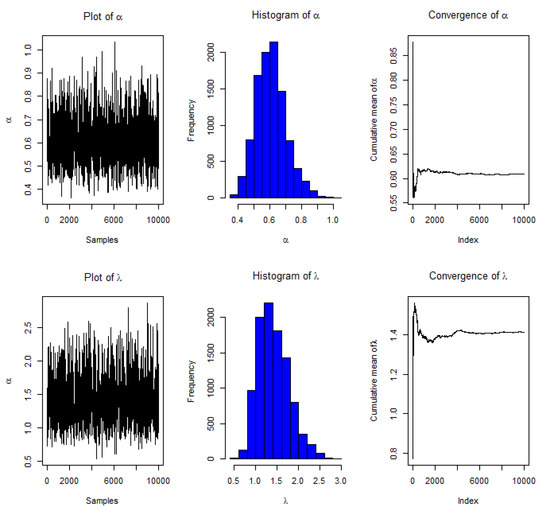
Figure 2. Convergence of MCMC estimates for $\alpha$ and $\lambda$ using MH algorithm under PT1C3 and $CT-I$ where $m=3$ and $n=50$.

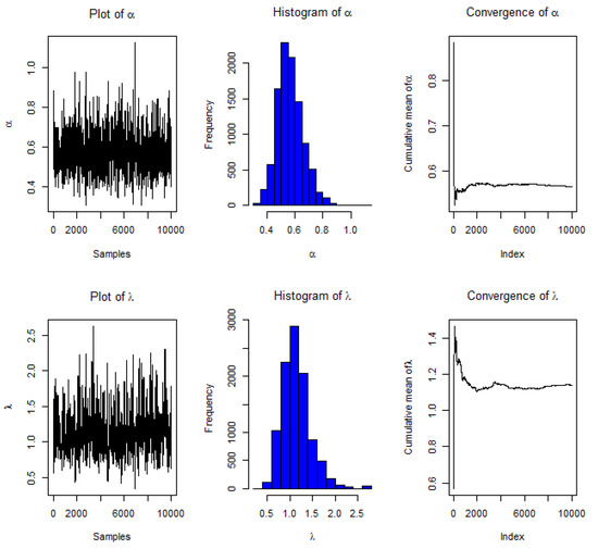
Figure 3. Plots of convergence of MCMC estimates for $\alpha$ and $\lambda$ by using MH algorithm under PT1C10 and $CT-IV$ where $m=4$ and $n=50$.

4.2. Real Data Analysis

The accompanying data set contains actual data on total yearly rainfall (inches) in January from 1880 to 1916. This is data was first analyzed by [9]. There were 37 observations listed below:

1.33, 1.43, 1.01, 1.62, 3.15, 1.05, 7.72, 0.20, 6.03, 0.25, 7.83, 0.25, 0.88, 6.29, 0.94, 5.84, 3.23, 3.70, 1.26, 2.64, 1.17, 2.49, 1.62, 2.10, 0.14, 2.57, 3.85, 7.02, 5.04, 7.27, 1.53, 6.70, 0.07, 2.01, 10.35, 5.42, 13.3.

We begin by determining if the NH distribution is appropriate for evaluating this data set. The computed Kolmogorov–Smirnov (K-S) for the NH model for the given data set is 0.091 and its p-value is 0.9 where $\hat{\alpha }=1.2557$ and $\hat{\lambda }=0.1976$ this implies that this distribution (NH) is a suitable model for the current data set.

From the original data we generate different PT1C samples. Removed items are considered as in simulation study in Table 1 for $n=25$. In addition, different stages of censoring are proposed at $m=3$ and $m=5$ and four CT $T_j$ proposed as follows:

• $CT-I=(0.90,1.32,3.20)$
• $CT-II=(1.15,2.49,5.84)$
• $CT-III=(0.25,1.25,1.65,2.65,5.20)$
• $CT-IV=(1.00,1.50,2.50,3.75,6.30)$

where $j=1,2,\dots ,m$. As discussed in simulation study, patterns $CT-I$ and $CT-II$ for $m=3$ and $CT-III$ and $CT-IV$ for $m=5$

We compute the MLErs of the parameters $\alpha$ and $\lambda$, as well as their corresponding 95% ACoI estimates. We also compute BEs under the informative prior using the MH technique. It should be noted that the non-informative prior is assumed for $a=b=c=d=0$. It is said that while using the MH method to generate samples from the posterior distribution, starting values of $(\alpha ,\lambda )$ are taken into account as $({\alpha }^{(0)},{\lambda }^{(0)})=(\hat{\alpha },\hat{\lambda })$, where $\hat{\alpha }$ and $\hat{\lambda }$ are the MLEs of the parameters $\alpha$ and $\lambda$, respectively. As a result, we investigated the variance–covariance matrix $S_{\theta }$ of $(ln(\hat{\alpha }),ln(\hat{\lambda }))$, which is readily produced using the delta approach. Ultimately, among many of the total 10,000 samples generated by the PD, we excluded 2000 burn-in samples and derived BEs and HPD interval estimates using the approach of [23].

All the estimated values of MLEs and ACoI and standard errors (St.Er) are mentioned in Table 8 and Table 9 for $m=3$ and $m=5$, receptively. In addition, Bayesian estimate using MCMC using the MH method, as well as accompanying HPD intervals and St.Er, are determined.

Table 8. ML and BEs with associated St.Er (in practices) and CoIs based on various PT1C schemes for given real data set at $m=3$.

Scheme	Parm.	MLE		Bayesian
$\mathcal{R}$		Estimate (St.Er)	ACoI	Estimate (St.Er)	HPD
CT-I = (0.90, 1.32, 3.20)
$(0^{\left(2\right)},R_m)$	$\alpha$	1.2296 (1.8636)	(1.0470, 1.4122)	1.1861 (0.0006)	(1.1481, 1.2533)
	$\lambda$	0.2032 (0.3842)	(0.1655, 0.2408)	0.1924 (0.0009)	(0.1508, 0.2544)
$(4^{\left(2\right)},R_m)$	$\alpha$	1.6752 (2.9794)	(1.3508, 1.9996)	1.6753 (0.0017)	(1.6061, 1.7412)
	$\lambda$	0.1604 (0.3372)	(0.1237, 0.1972)	0.1683 (0.0005)	(0.1296, 0.2100)
$(7^{\left(2\right)},R_m)$	$\alpha$	1.2462 (2.2382)	(0.9328, 1.5595)	1.2048 (0.0016)	(1.1379, 1.2686)
	$\lambda$	0.2021 (0.4354)	(0.1411, 0.2631)	0.1757 (0.0009)	(0.1135, 0.2203)
$(8,0,R_m)$	$\alpha$	1.0090 (1.6595)	(0.7588, 1.2593)	1.0965 (0.0011)	(1.0400, 1.1580)
	$\lambda$	0.2570 (0.5199)	(0.1787, 0.3354)	0.2605 (0.0010)	(0.1974, 0.3074)
$(14,0,R_m)$	$\alpha$	0.2412 (0.4808)	(0.1066, 0.3759)	0.1701 (0.0006)	(0.1201, 0.2144)
	$\lambda$	1.1757 (3.4147)	(0.2196, 2.1318)	1.1761 (0.0004)	(1.1341, 1.2161)
$(0,8,R_m)$	$\alpha$	1.2296 (1.8636)	(1.0470, 1.4122)	1.4097 (0.0042)	(1.2987, 1.5150)
	$\lambda$	0.2032 (0.3842)	(0.1655, 0.2408)	0.2098 (0.0006)	(0.1676, 0.2574)
$(0,14,R_m)$	$\alpha$	1.2436 (1.0165)	(1.0581, 1.4203)	1.2343 (0.0006)	(1.2022, 1.2899)
	$\lambda$	0.2103 (0.3755)	(0.1628, 0.2431)	0.2887 (0.0004)	(0.2508, 0.3257)
CT-II = (1.15, 2.49, 5.84)
$(0^{\left(2\right)},R_m)$	$\alpha$	0.6500 (0.3424)	(0.6232, 0.6769)	0.6510 (0.0008)	(0.5990, 0.7045)
	$\lambda$	0.4699 (0.4061)	(0.4380, 0.5017)	0.4640 (0.0008)	(0.4101, 0.5193)
$(4^{\left(2\right)},R_m)$	$\alpha$	0.7107 (0.4333)	(0.6703, 0.7512)	0.6445 (0.0040)	(0.5539, 0.7474)
	$\lambda$	0.4374 (0.4076)	(0.3993, 0.4754)	0.4977 (0.0007)	(0.4426, 0.5320)
$(7^{\left(2\right)},R_m)$	$\alpha$	0.6497 (0.5127)	(0.5905, 0.7088)	0.6690 (0.0006)	(0.6367, 0.7287)
	$\lambda$	0.4065 (0.4712)	(0.3521, 0.4608)	0.3936 (0.0004)	(0.3571, 0.4376)
$(8,0,R_m)$	$\alpha$	0.7105 (0.6098)	(0.6358, 0.7852)	0.6105 (0.0024)	(0.5415, 0.7027)
	$\lambda$	0.4065 (0.4932)	(0.3460, 0.4669)	0.4755 (0.0006)	(0.4161, 0.5227)
$(14,0,R_m)$	$\alpha$	1.2146 (3.3282)	(0.6710, 1.7582)	1.1291 (0.0011)	(1.0797, 1.2022)
	$\lambda$	0.1920 (0.6113)	(0.0922, 0.2919)	0.2766 (0.0003)	(0.2451, 0.3073)
$(0,8,R_m)$	$\alpha$	0.6500 (0.3424)	(0.6232, 0.6769)	0.6934 (0.0003)	(0.6586, 0.7263)
	$\lambda$	0.4699 (0.4061)	(0.4380, 0.5017)	0.4551 (0.0008)	(0.3929, 0.4878)
$(0,14,R_m)$	$\alpha$	0.6531 (0.3125)	(0.6177, 0.6697)	0.7151 (0.0003)	(0.6821, 0.7570)
	$\lambda$	0.4608 (0.4003)	(0.4016, 0.5720)	0.5392 (0.0004)	(0.5007, 0.5820)

Table 9. ML and BEs with associated St.Er (in practices) and CoIs based on various PT1C schemes for given real data set at $m=5$.

Scheme	Parm.	MLE		Bayesian
		Estimate (St.Er)	ACoI	Estimate (St.Er)	HPD
CT-III = (0.25, 1.25, 1.65, 2.65, 5.20)
$(0^{\left(4\right)},R_m)$	$\alpha$	0.6587 (0.3914)	(0.6268, 0.6907)	0.5277 (0.0015)	(0.4562, 0.5978)
	$\lambda$	0.4414 (0.4147)	(0.4076, 0.4753)	0.5009 (0.0005)	(0.4655, 0.5493)
$(2^{\left(4\right)},R_m)$	$\alpha$	0.6090 (0.3573)	(0.5740, 0.6442)	0.6432 (0.0005)	(0.6056, 0.6790)
	$\lambda$	0.5365 (0.4945)	(0.4881, 0.5853)	0.5626 (0.0023)	(0.4939, 0.6278)
$(4^{\left(4\right)},R_m)$	$\alpha$	0.4563 (0.3427)	(0.4083, 0.5043)	0.4308 (0.0018)	(0.3690, 0.5102)
	$\lambda$	0.6325 (0.7448)	(0.5282, 0.7367)	0.6371 (0.0010)	(0.5971, 0.7024)
$(8,0^{\left(3\right)},R_m)$	$\alpha$	0.4310 (0.2417)	(0.4031, 0.4588)	0.5241 (0.0024)	(0.4461, 0.5948)
	$\lambda$	0.7521 (0.7475)	(0.6659, 0.8382)	0.6555 (0.0049)	(0.5217, 0.7447)
$(16,0^{\left(3\right)},R_m)$	$\alpha$	0.6745 (0.4057)	(0.6215, 0.7275)	0.7709 (0.0039)	(0.6428, 0.8534)
	$\lambda$	0.5960 (0.5662)	(0.5220, 0.6700)	0.5178 (0.0017)	(0.4477, 0.5701)
$(0^{\left(3\right)},8,R_m)$	$\alpha$	0.7007 (0.4938)	(0.6546, 0.7468)	0.6742 (0.0051)	(0.5514, 0.7752)
	$\lambda$	0.4126 (0.4310)	(0.3723, 0.4528)	0.4383 (0.0004)	(0.4029, 0.4753)
$(0^{\left(3\right)},16,R_m)$	$\alpha$	0.9511 (1.1670)	(0.8240, 1.0782)	0.9558 (0.0003)	(0.9206, 0.9907)
	$\lambda$	0.2772 (0.4397)	(0.2294, 0.3251)	0.2855 (0.0005)	(0.2454, 0.3282)
CT-IV = (1.00, 1.50, 2.50, 3.75, 6.30)
$(0^{\left(4\right)},R_m)$	$\alpha$	0.7861 (0.4593)	(0.7527, 0.8194)	0.8090 (0.0004)	(0.7539, 0.8415)
	$\lambda$	0.3475 (0.3171)	(0.3245, 0.3705)	0.2486 (0.0011)	(0.2022, 0.3253)
$(2^{\left(4\right)},R_m)$	$\alpha$	0.8379 (0.6163)	(0.7830, 0.8928)	0.8335 (0.0004)	(0.7857, 0.8665)
	$\lambda$	0.3055 (0.3279)	(0.2762, 0.3347)	0.2796 (0.0005)	(0.2334, 0.3331)
$(4^{\left(4\right)},R_m)$	$\alpha$	0.6928 (0.5826)	(0.6256, 0.7600)	0.6745 (0.0003)	(0.6329, 0.7071)
	$\lambda$	0.3795 (0.4591)	(0.3266, 0.4324)	0.3897 (0.0003)	(0.3551, 0.4174)
$(8,0^{\left(3\right)},R_m)$	$\alpha$	0.9776 (0.8408)	(0.8991, 1.0561)	1.0171 (0.0014)	(0.9323, 1.0709)
	$\lambda$	0.2331 (0.2826)	(0.2067, 0.2595)	0.1931 (0.0005)	(0.1496, 0.2342)
$(16,0^{\left(3\right)},R_m)$	$\alpha$	0.9075 (0.7436)	(0.8164, 0.9986)	1.0106 (0.0017)	(0.9454, 1.0703)
	$\lambda$	0.2961 (0.3369)	(0.2548, 0.3373)	0.2874 (0.0005)	(0.2397, 0.3258)
$(0^{\left(3\right)},8,R_m)$	$\alpha$	0.9141 (0.7129)	(0.8559, 0.9723)	0.9017 (0.0013)	(0.8196, 0.9551)
	$\lambda$	0.2892 (0.3217)	(0.2629, 0.3154)	0.3447 (0.0003)	(0.3162, 0.3814)
$(0^{\left(3\right)},16,R_m)$	$\alpha$	1.1187 (1.3095)	(1.0021, 1.2350)	1.0883 (0.0004)	(1.0591, 1.1269)
	$\lambda$	0.2272 (0.3467)	(0.1963, 0.2581)	0.2419 (0.0003)	(0.2113, 0.2789)

5. Summary and Conclusions

Throughout this paper, we looked at the NH distribution estimate and prediction under PT1C from both a classical and a Bayesian approach. We obtained maximum likelihood estimates and ACIs for the unknown parameters of the NH distribution. Then, using informative priors, we generated Bayes estimates using MCMC approach as well as the corresponding HPD interval estimates. Furthermore, when an informative prior is used, a discussion of how to choose the values of hyper-parameters for a Bayesian estimate based on historical samples is discussed. The simulation results show that MLEs informative Bayes estimates under informative prior utilizing MCMC outperform MLEs. For future work, we will employ Bayesian estimation using the squared error loss function, although other loss functions can also be used. Furthermore, the current methodology might be extended to the development of an optimal progressive censoring sample strategy, as well as alternate censoring strategies.

References

- Nadarajah, S.; Haghighi, F. An extension of the exponential distribution. Stat. J. Theor. Appl. Stat. 2011, 45, 543–558. [Google Scholar] [CrossRef]
- Nikulin, M.; Haghighi, F. A chi-squared test for the generalized power Weibull family for the head-and-neck cancer censored data. J. Math. Sci. 2006, 133, 1333–1341. [Google Scholar] [CrossRef]
- Haghighi, F. Optimal design of accelerated life tests for an extension of the exponential distribution. Reliab. Eng. Syst. Saf. 2014, 131, 251–256. [Google Scholar] [CrossRef]
- Dey, S.; Zhang, C.; Asgharzadeh, A.; Ghorbannezhad, M. Comparisons of methods of estimation for the NH distribution. Ann. Data Sci. 2017, 4, 441–455. [Google Scholar] [CrossRef]
- Kumar, D.; Dey, S.; Nadarajah, S. Extended exponential distribution based on order statistics. Commun. Stat. Theory Methods 2017, 46, 9166–9184. [Google Scholar] [CrossRef]
- Kumar, D.; Malik, M.R.; Dey, S.; Shahbaz, M.Q. Recurrence relations for moments and estimation of parameters of extended exponential distribution based on progressive type-II right-censored order statistics. J. Stat. Theory Appl. 2019, 18, 171–181. [Google Scholar] [CrossRef] [Green Version]
- Singh, S.; Singh, U.; Kumar, M.; Vishwakarma, P. Classical and Bayesian inference for an extension of the exponential distribution under progressive type-II censored data with binomial removals. J. Stat. Appl. Probab. Lett. 2014, 1, 75–86. [Google Scholar] [CrossRef]
- Singh, U.; Singh, S.K.; Yadav, A.S. Bayesian estimation for extension of exponential distribution under progressive type-II censored data using Markov Chain Monte Carlo method. J. Stat. Appl. Probab. 2015, 4, 275–283. [Google Scholar]
- Selim, M.A. Estimation and prediction for Nadaraj ah–Haghighi distribution based on record values. Pak. J. Stat. 2018, 34, 77–90. [Google Scholar]
- Ashour, S.K.; El-Sheikh, A.A.; Elshahhat, A. Inferences and optimal censoring schemes for progressively first-failure censored Nadarajah–Haghighi distribution. Sankhya A 2020, 1–39. [Google Scholar] [CrossRef]
- Dey, S.; Wang, L.; Nassar, M. Inference on Nadarajah–Haghighi distribution with constant stress partially accelerated life tests under progressive type-II censoring. J. Appl. Stat. 2021, 1–22. [Google Scholar] [CrossRef]
- Wu, M.; Gui, W. Estimation and Prediction for NadarajahHaghighi Distribution under Progressive Type-II Censoring. Symmetry 2021, 13, 999. [Google Scholar] [CrossRef]
- Balakrishnan, N.; Han, D.; Iliopoulos, G. Exact inference for progressively type-I censored exponential failure data. Metrika 2011, 73, 335–358. [Google Scholar] [CrossRef]
- Korkmaz, M.C.; Yousof, H.M.; Rasekhi, M.; Hamedan, G.G. The odd Lindley Burr XII model: Bayesian analysis, classical inference and characterizations. J. Data Sci. 2018, 16, 327–354. [Google Scholar] [CrossRef]
- Yousof, H.M.; Korkmaz, M.C. Topp-Leone Nadaraj ah–Haghighi distribution. İstatistikçiler Dergisi İstatistik ve Aktüerya 2017, 10, 119–128. [Google Scholar]
- Balasooriya, U.; Low, C.K. Competing causes of failure and reliability tests for Weibull lifetimes under type I progressive censoring. IEEE Trans. Reliab. 2004, 53, 29–36. [Google Scholar] [CrossRef]
- Cohen, A.C. Progressively censored samples in life testing. Technometrics 1963, 5, 327–329. [Google Scholar] [CrossRef]
- Balakrishnan, N.; Cramer, E. The Art of Progressive Censoring: Applications to Reliability and Quality; Springer: New York, NY, USA, 2010. [Google Scholar]
- Mahmoud, R.M.; Muhammed. H.Z.; El-Saeed, A.R. Inference for generalized inverted exponential distribution under progressive Type-I censoring scheme in presence of competing risks model. Sankhya A Indian J. Stat. 2021. [Google Scholar] [CrossRef]
- Mahmoud, R.M.; Muhammed, H.Z.; El-Saeed, A.R. Analysis of progressively Type-I censored data in competing risks models with generalized inverted exponential distribution. J. Stat. Appl. Probab. 2020, 9, 109–117. [Google Scholar]
- Mahmoud, R.M.; Muhammed, H.Z.; El-Saeed, A.R.; Abdellatif, A.D. Estimation of parameters of the GIE distribution under progressive Type-I censoring. J. Stat. Theory Appl. 2021, 20, 380–394. [Google Scholar] [CrossRef]
- Algarni, A.; Elgarhy, M.; Almarashi, A.M.; Fayomi, A.; El-Saeed, A.R. Classical and Bayesian Estimation of the Inverse WeibullDistribution: Using Progressive Type-I Censoring Scheme. Adv. Civ. Eng. 2021, 2021, 5701529. [Google Scholar]
- Chen, M.H.; Shao, Q.M. Monte Carlo estimation of Bayesiancredible and HPD intervals. J. Comput. Graph. Stat. 1999, 6, 69–92. [Google Scholar]
Publisher’s Note: MDPI stays neutral with regard to jurisdictional claims in published maps and institutional affiliations. |
© 2022 by the authors. Licensee MDPI, Basel, Switzerland. This article is an open access article distributed under the terms and conditions of the Creative Commons Attribution (CC BY) license (https://creativecommons.org/licenses/by/4.0/).