Optimal Operation for Reduced Energy Consumption of an Air Conditioning System Using Neural Inverse Optimal Control

Abstract

For a comfortable thermal environment, the main parameters are indoor air humidity and temperature. These parameters are strongly coupled, causing the need to search for multivariable control alternatives that allow efficient results. Therefore, in order to control both the indoor air humidity and temperature for direct expansion (DX) air conditioning (A/C) systems, different controllers have been designed. In this paper, a discrete-time neural inverse optimal control scheme for trajectories tracking and reduced energy consumption of a DX A/C system is presented. The dynamic model of the plant is approximated by a recurrent high-order neural network (RHONN) identifier. Using this model, a discrete-time neural inverse optimal controller is designed. Unscented Kalman filter (UKF) is used online for the neural network learning. Via simulation the scheme is tested. The proposed approach effectiveness is illustrated with the obtained results and the control proposal performance against disturbances is validated.

1. Introduction

Not just a comfortable level of indoor air temperature is the only objective of air conditioning (A/C) systems [1,2]. Additionally, maintaining an adequate level of indoor air humidity is essential for an A/C system, since the efficient operation of building A/C systems, indoor air quality (IAQ) and building thermal comfort for occupants is directly affected by indoor humidity [3,4].

Recently, the use of direct expansion (DX) air conditioning (A/C) systems has had an exponential increase in different types of buildings small to medium scale [5,6]. More flexibility for installation, reduced operating cost and more energy savings, are advantages of the DX A/C, compared to chilled water based central A/C systems. Single speed compressors and fans, which rely on an on–off cycle to control indoor temperature only, are typical characteristics of conventional A/C systems [7]. The result is an indoor humidity imbalance, causing a thermal comfort unwanted level for the occupants [8]. However, by varying the fan speed and the compressor speed it is possible to control the humidity and air temperature simultaneously, achieving this with the development of variable speed (VS) driver technology [9]. For humidity and temperature control in air VS DX A/C, different control strategies have been designed and used, from the traditional proportional integral derivative (PID) control to advanced and robust controllers [10]. These include direct digital control [11], multi-input multi-output control method [12], neural network based [13,14,15], fuzzy logic controller (FLC) [16], Genetic and Swarm Algorithms [17] and Adaptive Control [18]. The development of those type of controllers requires a strong knowledge of mathematical modeling and advanced control techniques. In [19,20,21], control schemes that could be applied to the A/C system using fractional modeling are presented.

On the other hand, a control scheme based on plant dynamic model is necessary for realistic situations. This is a motivation to develop models based on an Artificial Neural Network (ANN) to model the plant dynamics to be controlled. Specifically, both for nonlinear process control and identification, ANN have been widely used. Feedforward ANN is one of the most popular for dynamical systems modeling, but the difficulties in the training step have limited its application [22]. When there is management of a state space structure, recurrent neural networks (RNN) have a better performance than classical feedback networks. However, when classical gradient optimization algorithms are used in its learning, its evolution is slow and very poorly approaches satisfactory results in longer input sequences, leading to a complicated numerical problem [23].

In contrast, the extended Kalman filter (EKF) algorithm has been introduced to train neural networks [24,25], with improved learning convergence [26]. Unfortunately, the EKF’s main drawback is the derivation of the Jacobian matrices, which can be complex, causing implementation difficulties [23,27]. Therefore, an unscented Kalman Filter (UKF) is proposed to solve the EKF’s problems. UKF is a filtering algorithm which uses Unscented Transformation (UT) [28]. The essential difference between EKF and UKF systems is the representation of Gaussian Random Variables (GRV) for propagation through system dynamics [29].

Therefore, a RHONN is proposed to identify the dynamic model for VS DX A/C system, assuming all the states available to be measured. The algorithm implemented for the RHONN learning uses UKF.

Determining control signals which will allow a process to comply with physical constraints and minimize a cost functional simultaneously is the optimal control theory objective [30]. Unfortunately, the difficult and complex process of solving the Hamilton Jacobi Bellman (HJB) equation is required, an alternative to avoid solving the HJB equation is to use the inverse optimal control [31].

Before establishing that the control optimizes a cost functional, a stabilizing feedback control must be developed, according to the inverse approach. The determination a posteriori of the cost functional for the stabilizing feedback control law is an essential feature of the inverse approach [24,32].

Applications of this complete control scheme are illustrated in: [33], where an optimal inverse neural control for discrete-time impulsive systems is determined. Reference [34] presents a discrete-time inverse optimal control scheme for a doubly-fed induction generator using a neural network. One more example in [35] where a neural controller for an induction motor is synthesized.

All the characteristics and strengths mentioned motivate the realization of this research work, since it allows establishing a multivariable and robust control technique, capable of tracking thermal profiles established by a user and rejecting both external and internal disturbances. This creates conditions for adequate energy consumption and thermal comfort. Furthermore, this optimal operation is reflected in the control signals generated by the proposed scheme.

Section 2 presents the methodology to obtain a VS DX A/C system mathematical model. Then, a brief review of the discrete-time neural identification for nonlinear systems is described, followed by a section where the inverse optimal controller is established. Section 3 shows the results and discussions that illustrate the application of the proposed inverse optimal control and neural identifier employing simulations. The last section presents the conclusions of this work.

2. Methodology

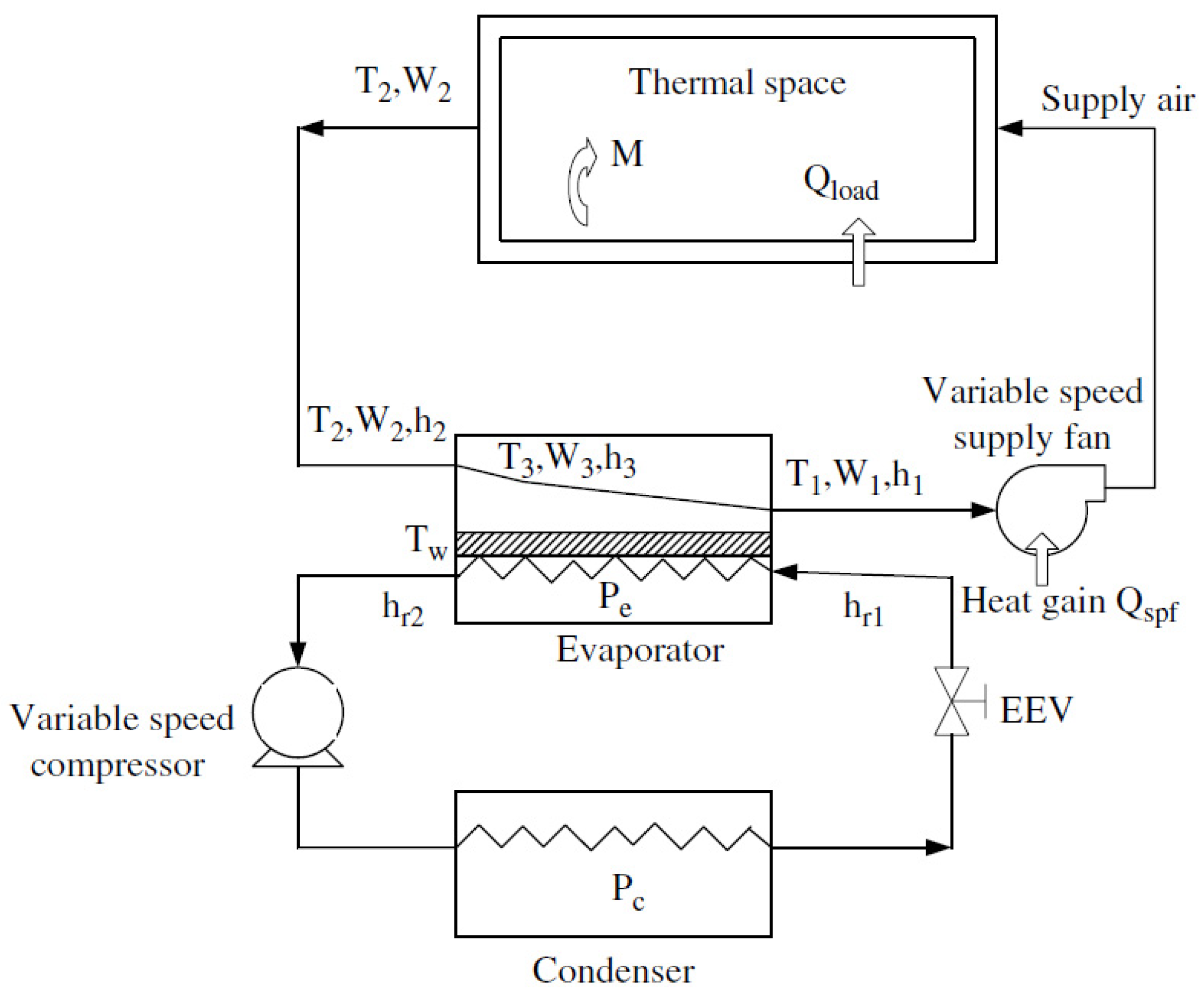
2.1. The Experimental VS DX A/C System and Its Dynamic Modeling

An air distribution sub-system (air side) and a DX refrigeration plant (refrigerant side) are the main components of the experimental VS DX A/C system, as shown simplified schematic diagram in Figure 1. An electronic expansion valve (EEV), a variable-speed rotor compressor, an air-cooled tube-plate-finned condenser and a high-efficiency tube-louver-finned DX evaporator are major elements that make up the DX refrigeration plant.

Figure 1. Schematic diagram of the experimental VS DX A/C system.

The energy and mass conservation principles are used mainly to obtain the mathematical model of the VS DX A/C system. Further, for the development of the mathematical model, it should be considered: (a) the thermal losses in air ducts are negligible; (b) two regions; dry-cooling region and wet-cooling region on the airside of the DX evaporator; and (c) no fresh air intake to the system and the perfect air mixing inside all heat exchangers and the thermal space [12,36].

The mathematical model complete analysis is presented in [36], obtaining the following equations.

$$C_p\rho V\frac{d{T}_2}{dt}=C_p\rho (T_1-T_2)f+Q_{spf}+Q_{load},$$

(1)

$$\rho V\frac{d{W}_2}{dt}=\rho (W_1-W_2)f+M,$$

(2)

$$C_p\rho V_{h_1}\frac{d{T}_3}{dt}=C_p\rho (T_2-T_3)f+{\alpha }_1{A}_1\left(T_W-\frac{T_2+T_3}{2}\right),$$

(3)

$$C_p\rho V_{h_2}\frac{d{T}_1}{dt}+\rho V_{h_2}{h}_{fg}\frac{d{W}_1}{dt}=C_p\rho (T_3-T_1)f+\rho h_{fg}(W_2-W_1)f+{\alpha }_2{A}_2\left(T_W-\frac{T_3+T_1}{2}\right),$$

(4)

$${\left(C_p\rho V\right)}_W\frac{d{T}_W}{dt}={\alpha }_1{A}_1\left(\frac{T_2+T_3}{2}-T_W\right)+{\alpha }_2{A}_2\left(\frac{T_3+T_1}{2}-T_W\right)-M_{ref}{}^{-1}\left(h_{r_2}-h_{r_1}\right),$$

(5)

$$\frac{\frac{d{W}_1}{dt}-(a{T}_1+b)\frac{d{T}_1}{dt}}{c}=0.$$

(6)

All model parameters are defined in the nomenclature, before references section. The dynamic model for the experimental VS DX A/C system is formed by Equations (1)–(6) and its state space representation in a compact format is given by:

$$\dot{x}=g(x,u)$$

(7)

where the state variables x = [x₁ x₂ x₃ x₄ x₅ x₆]^T = [T₁ T₂ T₃ T_w W₁ W₂]^T, the output variables y = [T₂ W₂]^T, input variables u = [u₁ u₂]^T = [f s]^T, and the function g(x,u), define the dynamic system, respectively.

g(x,u) is defined as follows:

$$g(x,u)=\left[\begin{array}{c}\frac{u_1(h_{fg}(x_6-x_5)+(x_3-x_1)C_p)\rho +g_2(x)A_2{\alpha }_2}{\rho V_{h_2}\left(g_1(x)h_{fg}+C_p\right)}\\ \frac{u_1(k_{spl}+C_p(x_1-x_2)\rho )+Q_{load}}{\rho C_{p}V}\\ \frac{g_3(x){\alpha }_1{A}_1+u_1{C}_p(x_2-x_3)\rho }{C_p\rho V_{h_1}}\\ \frac{{\alpha }_1{A}_1{g}_4(x)+{\alpha }_2{A}_2{g}_5(x)-\frac{V_{com}}{v_s\lambda }\left(h_{r_2}-h_{r_1}\right)u_2}{{\left(\rho C_{p}V\right)}_W}\\ \frac{(C_p(x_3-x_1)+u_1{h}_{fg}(x_6-x_5))\rho +{\alpha }_2{A}_2{g}_2(x)}{\rho V_{h_2}\left(Cp+h_{fg}{g}_1(x)\right)}{g}_1(x)\\ \frac{\rho (x_5-x_6)u_1+M}{\rho V}\end{array}\right],$$

(8)

with

$g_1(x)=\frac{a{x}_1+b}{c}$, $g_2(x)=x_4-\frac{x_3+x_1}{2}$,

$g_3(x)=x_4-\frac{x_2+x_3}{2}$, $g_4(x)=\frac{x_2+x_3}{2}-x_4$, $g_5(x)=\frac{x_3+x_1}{2}-x_4$

where

$a=0.0396,b=0.085,c=1000$.

The relationship between input variables and state variables is nonlinear, therefore Equation (7) is nonlinear.

In [36], the detailed validation of the above mathematical model for the VS DX A/C experimental system is reported.

2.2. Discrete-Time High-Order Neural Network

For pattern recognition and static systems modeling, multilayer neural networks are commonly used, since input and output mapping is learned through neural network (NN) training. A neural network, even with a single hidden layer, has the ability to uniformly approximate any continuous function over a compact domain, considering that there are enough synaptic connections in the NN, this fact has been demonstrated in different theoretical works.

Recurrent High-Order Neural Networks (RHONN) are considered extensions of the first order Hopfield model. They are used in control tasks due to their high number of interactions between neurons, as proposed in [37,38]. In addition, the RHONN model is flexible and allows incorporating a priori information about the structure of the system in the neural model.

2.2.1. Nonlinear System Neural Identification

The MIMO nonlinear in Equation (7) is identified using a RHONN defined as

$${\chi }_{k+1}=w_i^T{\phi }_i(x_k,u_k),$$

(9)

where χ is state vector of neurons that identifies the i-th component of state vector x in (7), x_k = [x_1,k x_2,k … x_n,k]^T, w_i is the respective online adapted weight vector, I = 1,…n; and u_k = [u₁,_k u_2,k… u_m,k]^T is the input vector to the neural network; φ is an L_p dimensional vector defined as

$${\phi }_i(x_k,u_k)=\left[\begin{array}{c}{\phi }_{i_1}\\ {\phi }_{i_2}\\ ⋮\\ {\phi }_{i_{Lp}}\end{array}\right]=\left[\begin{array}{c}{\displaystyle {\prod }_{j\in I_1}{Z}_{i_j}^{d_{i_j}(1)}}\\ {\displaystyle {\prod }_{j\in I_2}{Z}_{i_j}^{d_{i_j}(2)}}\\ ⋮\\ {\displaystyle {\prod }_{j\in I_{Lp}}{Z}_{i_j}^{d_{i_j}(L_p)}}\end{array}\right],$$

(10)

where L_p is the number p of high order connections, d_ij are nonnegative integers, and {I₁, I₂, … I_Lp} is a collection of unordered subsets of {1, 2, …, n + m}. Here Z_i is a vector defined as

$$Z_i=\left[\begin{array}{c}{Z}_{i_1}\\ ⋮\\ Z_{i_n}\\ Z_{i_{n+1}}\\ ⋮\\ Z_{i_{n+m}}\end{array}\right]=\left[\begin{array}{c}S(x_{1,k})\\ ⋮\\ S(x_{n,k})\\ u_{1,k}\\ ⋮\\ u_{m,k}\end{array}\right].$$

(11)

From Equation (11), the input vector to the neural network is u_k = [u_1,k, u_2,k, …, u_m,k]^⊤. S(•) is defined by

$$S(\varsigma )=\frac{e^{\varsigma }-e^{-\varsigma }}{e^{\varsigma }+e^{-\varsigma }},$$

(12)

where ς is any real value.

The unscented Kalman filter (UKF) algorithm [28] is used to train the RHONN identifier.

2.2.2. The UKF Training Algorithm

For recurrent neural networks (RNN), the best well-known training approach is the backpropagation through time learning [39]. Unfortunately, a first order gradient descent method such as backpropagation can have a very slow learning speed [26]. However, the Kalman filter (KF) as an algorithm for state / parameter estimation has become popular in the last four decades. This filter is especially useful for real-time applications, due to its easy implementation and computationally efficient calculation [23,27]. Nevertheless, for state estimation, especially of nonlinear systems, the original KF is often not good enough, according to the research community. The extended Kalman filter (EKF) is an extension of the KF to deal the non-linear system through a linearization procedure [27].

The unscented Kalman filter (UKF) is the nonlinear generalization of KF, which has several successful applications, such as recurrent neural network training [40]. Both the UKF and the EKF are conceptually similar, having the same basic principle, but the implementation is significantly different; only function evaluations instead of Taylor approximation, and no derivatives are needed (i.e., Jacobian or Hessian calculation).

A relatively new method for calculating the random variable statistics, which undergone a nonlinear transformation is called the unscented transformation (UT) and is used by the UKF [23]. The UT is UKF central technique used to handle the nonlinearity in a nonlinear transformation y = f(x), where f is an L × 1 vector-valued function, x and y are L × 1 vectors. Here, x is a random variable assumed to be normally distributed (Gaussian) with covariance P_x, and mean $\overline{\mathit{x}}$. An approach that replaces analytical linearization is provided by the UT which offers a statistical alternative, where the EKF Jacobian matrices are used. In [41] a detailed analytical comparison about linearization techniques is presented. The sigma-points used by UT are small set of points selected based on the a priori conditions, i.e., from the assumed prior distribution, the points are selected. Based on the selected scaling parameters for the UT, the confidence level from prior distribution or the sigma-points spread is determined. For the scaling parameters, there are different representations and notations. These representations are equivalent and affect both the sigma-points spread and the weight vectors used to reconstruct the a posteriori statistics (after the transformation).

Using three scaling parameters, the UT scaling can be represented fully [28,42]. α is the primary scaling parameter and determines the sigma-points spread. The α parameter has a variation range from 10-4 to 1. A wider sigma-points spread is caused by larger α, while a tighter (closer) sigma-points spread is the result of smaller α. The β parameter is used to include information about the prior distribution and is the secondary scaling parameter (β = 2 is optimal, for Gaussian distributions). The κ parameter is usually set to 0 and is the third scaling parameter [28]. In addition to the three parameters mentioned, a scaling parameter, λ, and two weight vectors, η^c (covariance) and η^m (mean) are defined

$$\begin{array}{l}\lambda ={\alpha }^2(L+\kappa )-L ,\\ {\mathit{\eta }}_0^m=\frac{\lambda }{L+\lambda } ,\\ {\mathit{\eta }}_0^c=\frac{\lambda }{L+\lambda }+1-{\alpha }^2+\beta ,\\ {\mathit{\eta }}_i^m={\mathit{\eta }}_i^c=\frac{1}{2(L+\lambda )},i=1,\dots ,2L ,\end{array}$$

(13)

where L is the state vector length. Then to generate 2L + 1 sigma-points, the prior mean $\overline{\mathit{x}}$, the covariance P_x and the parameter λ of the random variable x are used, as in

$$\mathit{\chi }=\left[\begin{array}{ccc}\overline{\mathit{x}}& \overline{\mathit{x}}+\sqrt{L+\lambda }\sqrt{{\mathit{P}}_x}& \overline{\mathit{x}}-\sqrt{L+\lambda }\sqrt{{\mathit{P}}_x}\end{array}\right].$$

(14)

Here χ is an L × (2L +1) matrix of sigma-points, where each sigma-point is represented by a column of this matrix, note that in Equation (14), the sum of a vector to each of the matrix columns defines the sum of a vector and matrix. Alternatively, an L × L matrix can be used for standard matrix addition, as long as the L × 1 column vector $\overline{\mathit{x}}$ can be multiplied with a 1 × L row vector of ones. It is also possible to notice that (14) contains the square root of a matrix. While there are different methods of calculating a matrix square root, the Cholesky ones is the recommended both in terms of computational efficiency and performance [43]. Here, the Cholesky decomposition is used to calculate a lower triangular matrix, and can then be used as a matrix square root representation, i.e.,

$${\mathit{P}}_x=\left(\sqrt{{\mathit{P}}_x}\right){\left(\sqrt{{\mathit{P}}_x}\right)}^T,$$

(15)

where $\sqrt{{\mathit{P}}_x}$ is a lower triangular matrix. Note that a principal matrix square root is different from this representation, which takes the form of Equation (15) that generally is non-triangular and without the transpose. Other method, called the “square-root UKF (SR-UKF)”, of handling the matrix square root was proposed [44], which can obtain different performance results, but has improved computational complexity.

Each point is passed through the nonlinear function, once the sigma-points have been generated, i.e., each column of the sigma-point matrix, χ, is propagated through the nonlinearity, as in

$${\mathsf{\psi }}^{\left(i\right)}=f({\mathit{\chi }}^{(i)}),i=0,1,\dots ,2L,$$

(16)

where the superscript (i) corresponds to the ith column of the matrix, whereas ψ is a matrix of transformed sigma-points. Then, the mean and covariance, using weighted averages, are estimated of these transformed sigma-points using the weight vectors that were defined in Equation (13), as in

$$\begin{array}{l}\overline{y}\approx {\displaystyle \sum _{i=0}^{2L}{\mathit{\eta }}_i^m}{\mathsf{\psi }}^{\left(i\right)} ,\\ {\mathit{P}}_y\approx {\displaystyle \sum _{i=0}^{2L}{\mathit{\eta }}_i^c\left({\mathsf{\psi }}^{\left(i\right)}-\overline{y}\right)}{\left({\mathsf{\psi }}^{\left(i\right)}-\overline{y}\right)}^T ,\end{array}$$

(17)

where P_y is the estimated covariance matrix of y, and $\overline{y}$ their estimated mean. These values correspond to the estimated statistical properties after the nonlinear transformation, or a posteriori statistics.

2.3. Inverse Optimal Control Introduction

Consider the following an affine discrete nonlinear system

$${\theta }_{k+1}=f({\theta }_k)+g({\theta }_k)u_k\hspace{1em}{\theta }_0=\theta (0),$$

(18)

where ${\theta }_k\in {ℝ}^n$ is the state of system at time $k\in \mathbb{N}$, $u\in {ℝ}^m$, $f:{ℝ}^n\to {ℝ}^n$, $g:{ℝ}^n\to {ℝ}^{n\times m}$, are smooth and bounded mapping. f(0) = 0 is assumed, and $\mathbb{N}$ denotes the nonnegative integers set. The trajectory tracking for the system is associated to the following meaningful cost functional in Equation (18)

$$\ell ({\vartheta }_k)={\displaystyle \sum _{n=k}^{\infty }(l({\vartheta }_n)+u_n^{T}R{u}_n)},$$

(19)

where ${\vartheta }_k={\theta }_k-{\theta }_{\delta ,k}$ with ${\theta }_{\delta ,k}$ as the desired trajectory for θ_k; ${\vartheta }_k\in {ℝ}^n; \ell ({\vartheta }_k):{ℝ}^n\to {ℝ}^{+}; l({\vartheta }_k):{ℝ}^n\to {ℝ}^{+}$ is a positive semidefinite function and $R:{ℝ}^n\to {ℝ}^{m\times m}$ is a real symmetric positive definite weighting matrix. The cost functional of Equation (19) is a performance measure [30]. To vary the weighting on control efforts according to the state value, the R entries can be functions of the system state, although they can also be fixed [30]. We assume that the full state θ_k is available, considering the state feedback control design problem.

Utilizing the optimal value function ${\ell }^{*}({\theta }_k)$ for (18) as Lyapunov function V(θ_k), Equation (19) can be rewritten as

$$V({\vartheta }_k)=l({\vartheta }_k)+u_k^{T}R{u}_k+{\displaystyle \sum _{n=k}^{\infty }(l({\vartheta }_n)+u_n^{T}R{u}_n)}=l({\vartheta }_k)+u_k^{T}R{u}_k+V({\vartheta }_{k+1}),$$

(20)

that requires the boundary condition V(0) = 0, to $V({\vartheta }_k)$ becomes a Lyapunov function. From Bellman optimality principle [45,46], it is known that, for the infinite horizon optimization case, the value function $V({\vartheta }_k)$ satisfies the discrete-time Bellman equation and becomes time-invariant [45,47,48]

$$V*({\vartheta }_k)=\underset{u_k}{\min }\left\{l({\vartheta }_k)+u_k^{T}R{u}_k+V*({\vartheta }_{k+1})\right\},$$

(21)

where $V*({\vartheta }_{k+1})$ depends on both ${\vartheta }_k$ and u_k through of ${\vartheta }_{k+1}$ in (18). Note that the Bellman equation is solved backward in time [47]. It is defined the discrete-time Hamiltonian H(${\vartheta }_k$, u_k ), in order to establish the conditions that the optimal control law must satisfy, as

$$H({\vartheta }_k,u_k)=l({\vartheta }_k)+u_k^{T}R{u}_k+V({\vartheta }_{k+1})-V({\vartheta }_k).$$

(22)

The optimal control law should satisfy $\frac{\partial H({\vartheta }_k,u_k)}{\partial u_k}=0$, that it is a necessary condition, then

$$0=2R{u}_k+\frac{\partial V({\vartheta }_{k+1})}{\partial u_k}=2R{u}_k+\frac{\partial {\vartheta }_{k+1}}{\partial u_k}\frac{\partial V({\vartheta }_{k+1})}{\partial {\vartheta }_{k+1}}=2R({\vartheta }_k)u_k+g^T({\theta }_k)\frac{\partial V({\vartheta }_{k+1})}{\partial {\vartheta }_{k+1}}.$$

(23)

Therefore, to achieve trajectory tracking, the optimal control law is formulated as

$$u_k^{*}=-\frac{1}{2}{R}^{-1}{g}^T({\theta }_k)\frac{\partial V({\vartheta }_{k+1})}{\partial {\vartheta }_{k+1}},$$

(24)

with the boundary condition V(0) = 0. It is necessary to solve the following HJB equation, for solving the trajectory tracking inverse optimal control problem

$$\begin{array}{l}0=l({\vartheta }_k)+V({\vartheta }_{k+1})-V({\vartheta }_k)+\frac{1}{4}\frac{\partial V^T({\vartheta }_{k+1})}{\partial {\vartheta }_{k+1}}g({\theta }_k)R^{-1}{g}^T({\theta }_k)\frac{\partial V({\vartheta }_{k+1})}{\partial {\vartheta }_{k+1}},\end{array}$$

(25)

which is a challenging task. It is proposed to solve the inverse optimal control problem.

Definition 1. 

Consider the tracking error [30] as ${\vartheta }_k={\theta }_k-{\theta }_{\delta ,k}$, θ_δ,k being the desired trajectory for θ_k. Let’s define the control law

$$u_k^{*}=-\frac{1}{2}{R}^{-1}{g}^T({\theta }_k)\frac{\partial V({\vartheta }_{k+1})}{\partial {\vartheta }_{k+1}}.$$

It will be inverse optimal (globally) stabilizing along the desired trajectory θ_δ,k if:

i.

It achieves (global) asymptotic stability of θ_k = 0 for system (18) along reference θ_δ,k;

ii.

$V({\vartheta }_k)$is (radially unbounded) positive definite function such that inequality

$$\overline{V}:=V({\vartheta }_{k+1})-V({\vartheta }_k)+u_k^{*T}R({\vartheta }_k)u_k^{*}\le 0,$$

(26)

is satisfied.

If chosen $l({\vartheta }_k):=-\overline{V}$, then $V({\vartheta }_k)$ is a solution for Equation (25), and cost functional Equation (19) is minimized.

Definition 1 establishes that, the knowledge of $V({\vartheta }_k)$ is basis to formulate the inverse optimal control law for trajectory tracking. Then, a control Lyapunov function (CLF) $V({\vartheta }_k)$ can be proposed, such that (i) and (ii) are guaranteed. Hence, instead of solving Equation (25) for $V({\vartheta }_k)$ a quadratic candidate CLF $V({\vartheta }_k)$ for Equation (24) is proposed with the form

$$V({\vartheta }_k)=\frac{1}{2}{\vartheta }_k^{T}P{\vartheta }_k,\hspace{1em}P=P^T>0,$$

(27)

to ensure stability of the tracking error ${\vartheta }_k$, where

$${\vartheta }_k={\theta }_k-{\theta }_{\delta .k}=\left[\begin{array}{c}{\theta }_{1,k}-{\theta }_{1\delta .k}\\ ⋮\\ {\theta }_{n,k}-{\theta }_{n\delta .k}\end{array}\right].$$

(28)

It is referred to as the inverse optimal control law, to the control law in Equation (24) with Equation (27) and it optimizes the meaningful cost functional of Equation (19). Consequently, by considering $V({\vartheta }_k)$ as in Equation (27), control law in Equation (24) takes the following form

$$\begin{array}{ll}{u}_k^{*}& =-\frac{1}{4}{R}^{-1}{g}^T({\theta }_k)\frac{\partial {\vartheta }_{{}_{k+1}}^{T}P{\vartheta }_{k+1}}{\partial {\vartheta }_{k+1}}=-\frac{1}{2}{R}^{-1}{g}^T({\theta }_k)P{\vartheta }_{k+1}\\ & =-\frac{1}{2}{\left(R+\frac{1}{2}{g}^T({\theta }_k)Pg({\theta }_k)\right)}^{-1}{g}^T({\theta }_k)P\left(f({\theta }_k)-{\theta }_{\delta ,k+1}\right).\end{array}$$

(29)

The existence of the inverse in Equation (29) is ensured, since P and R are symmetric matrices and positive definite.

3. Results and Discussion

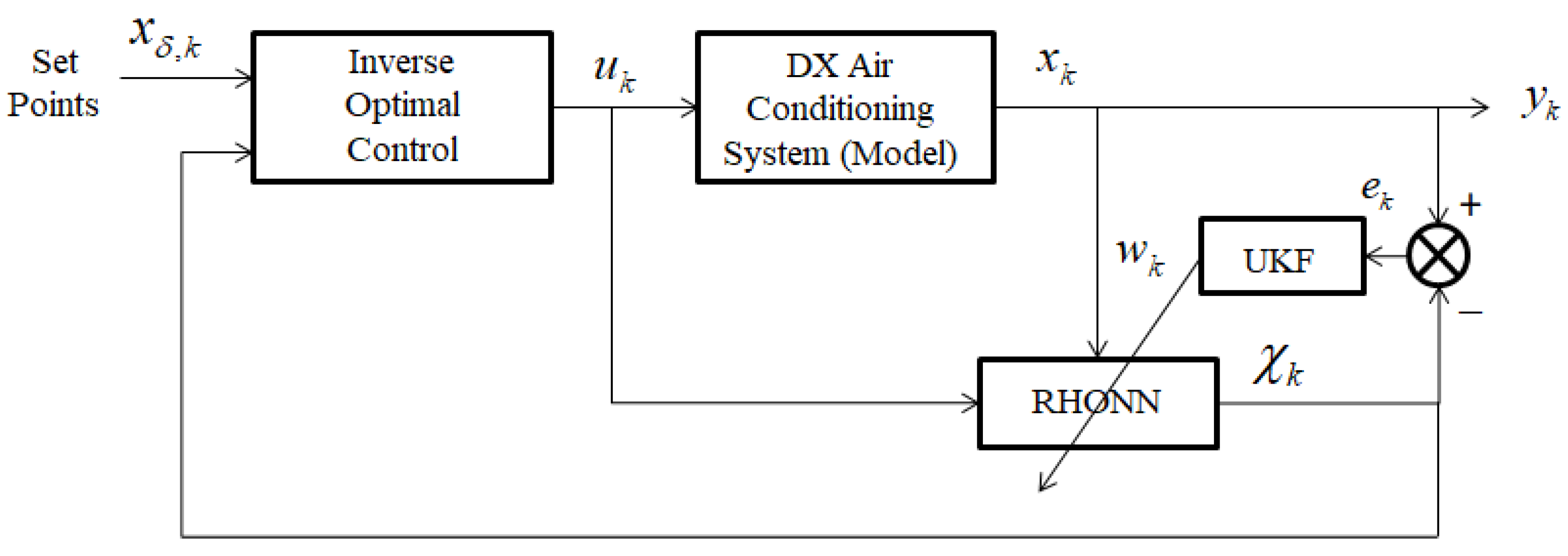
3.1. Identification and Control Scheme Application

The complete identification and control scheme is shown in Figure 2. This scheme main components are the VS DX A/C system model, the inverse optimal controller, and the neural identifier.

Figure 2. Proposed identification and control scheme.

Via simulation, the identification and control scheme are applied to the dynamic model for the VS DX A / C system. The mentioned model is formed by Equations (1)–(6).

Applying the neural identifier developed in Section 2.2.1, it is possible to obtain for the VS DX A/C system a discrete-time neural reduced model which uses UKF for training, as follows

$$\begin{array}{l}{\chi }_{{}_{1,k+1}}^{}=w_{11,k}S(x_{2,k}^{})+w_{12k}{x}_{6,k}^{}+w_1{u}_{2,k}^{} ,\\ {\chi }_{{}_{2,k+1}}^{}=w_{21,k}S(x_{2,k}^{})+w_{22k}S(x_{6,k}^{})+w_2{u}_{1,k}^{} ,\end{array}$$

(30)

where χ₁ and χ₂ identify the air temperature in the conditioned space x₂ and moisture content of air-conditioned space x₆, respectively. The NN training is performed online and all its states are initialized in random way. The parameter selection of the RHONN identifier is heuristic as

$$\begin{array}{llll}L=2& \alpha =1\times {10}^{-3}& \beta =0.5& \kappa =1\\ R_1=0.1& R_2=0.1& Q_1=0.1I& Q_2=0.1I\\ w_1=0.1& w_2=0.1& & \end{array}$$

where I is the 2 × 2 identity matrix. The neural network structure in Equation (30) is chosen as in [25] in order to minimize the state estimation error.

Using the control laws described in Section 2.3, the desired reference trajectories x_1δ,k and x_2δ,k are tracked by the states χ_1,k and χ_2,k, respectively. Applying Equation (29), it is possible to do this as follows

$$u_k=-\frac{1}{2}{\left(R+\frac{1}{2}{g}^T({\chi }_k)Pg({\chi }_k)\right)}^{-1}\times g^T({\chi }_k)P\left(f({\chi }_k)-x_{\delta ,k+1}\right),$$

(31)

where the P and R selection is completed heuristically as

$$P=\left[\begin{array}{cc}1275& 750\\ 750& 1275\end{array} \right]\hspace{1em}R=2\times {10}^{-2}I.$$

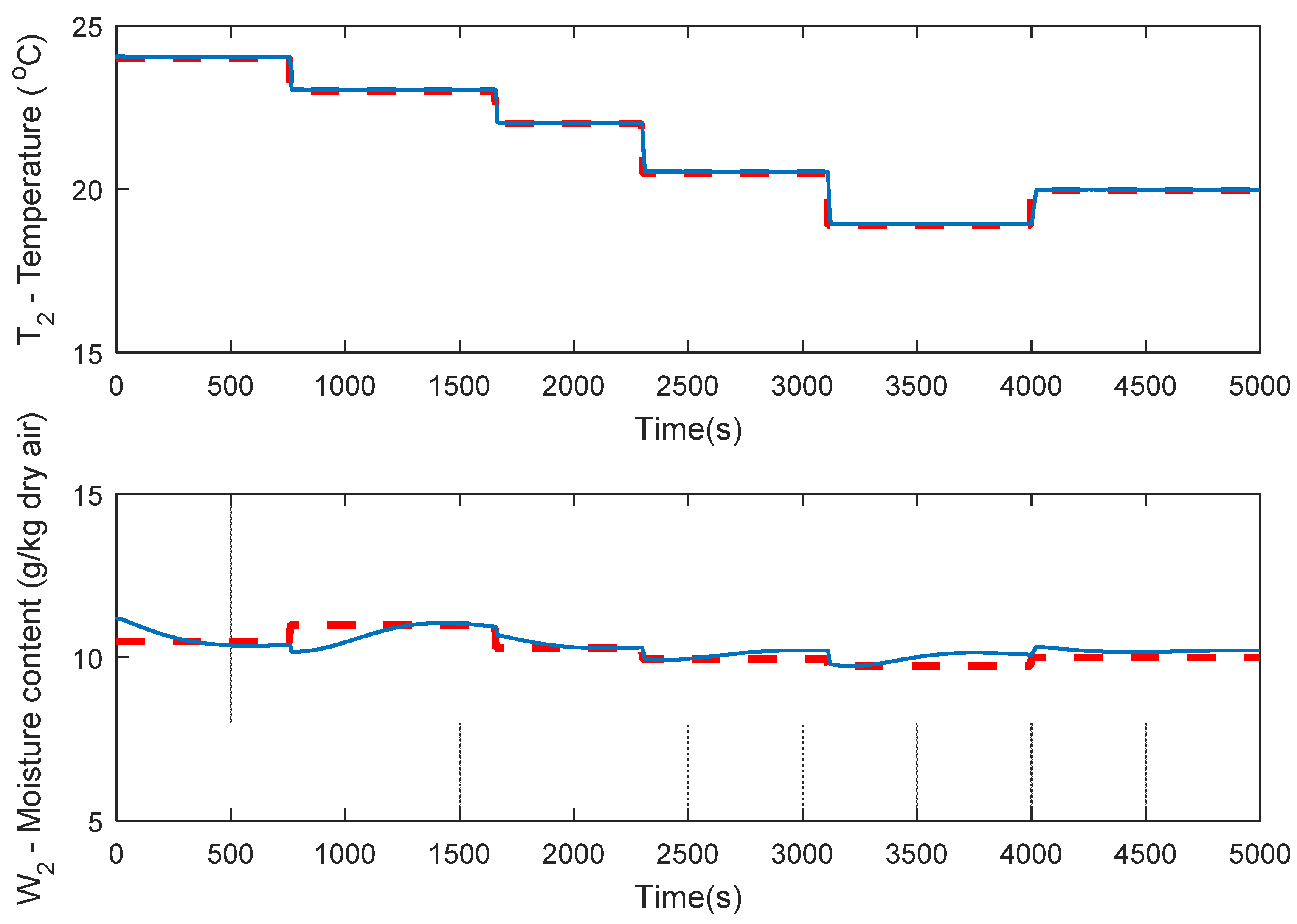
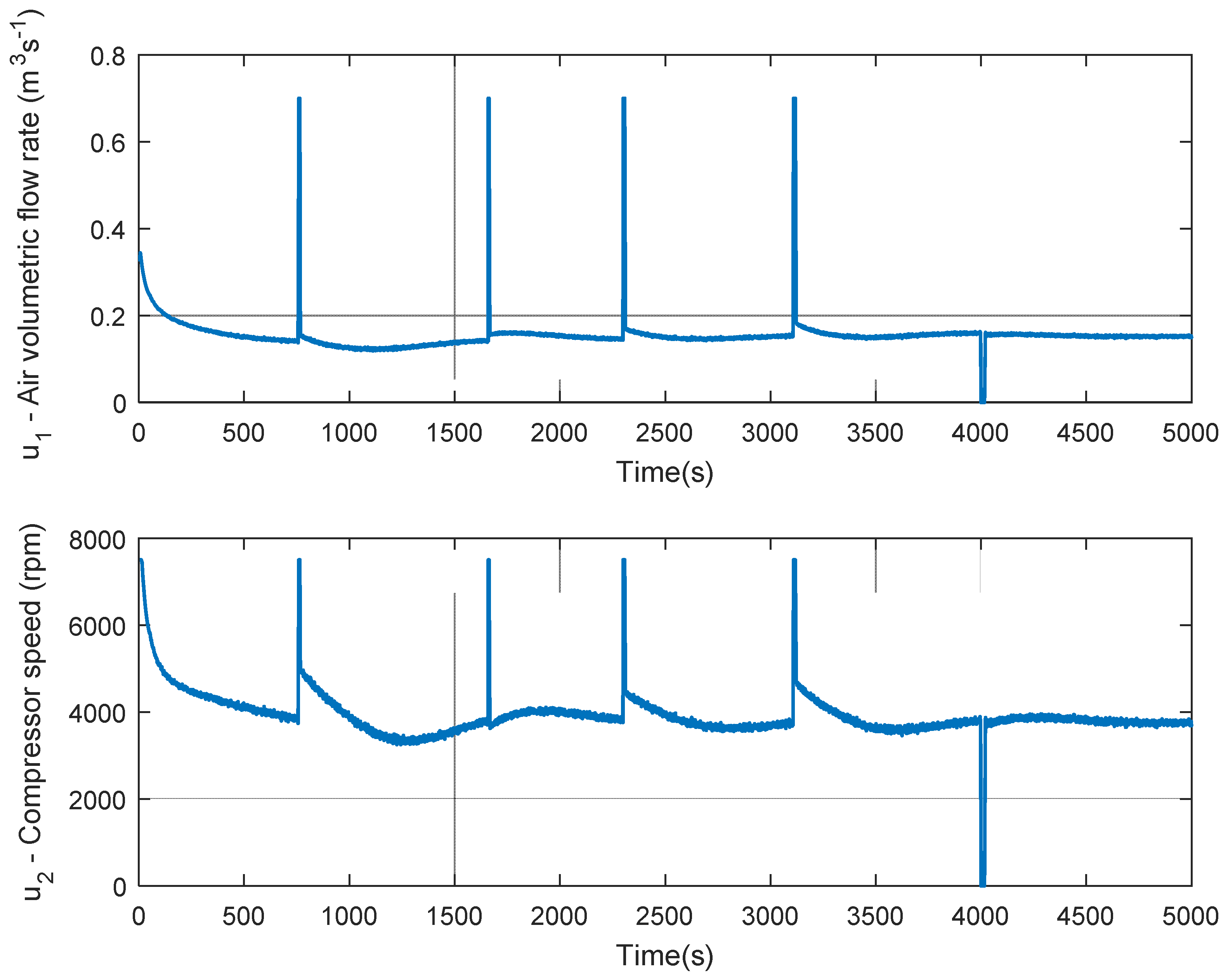
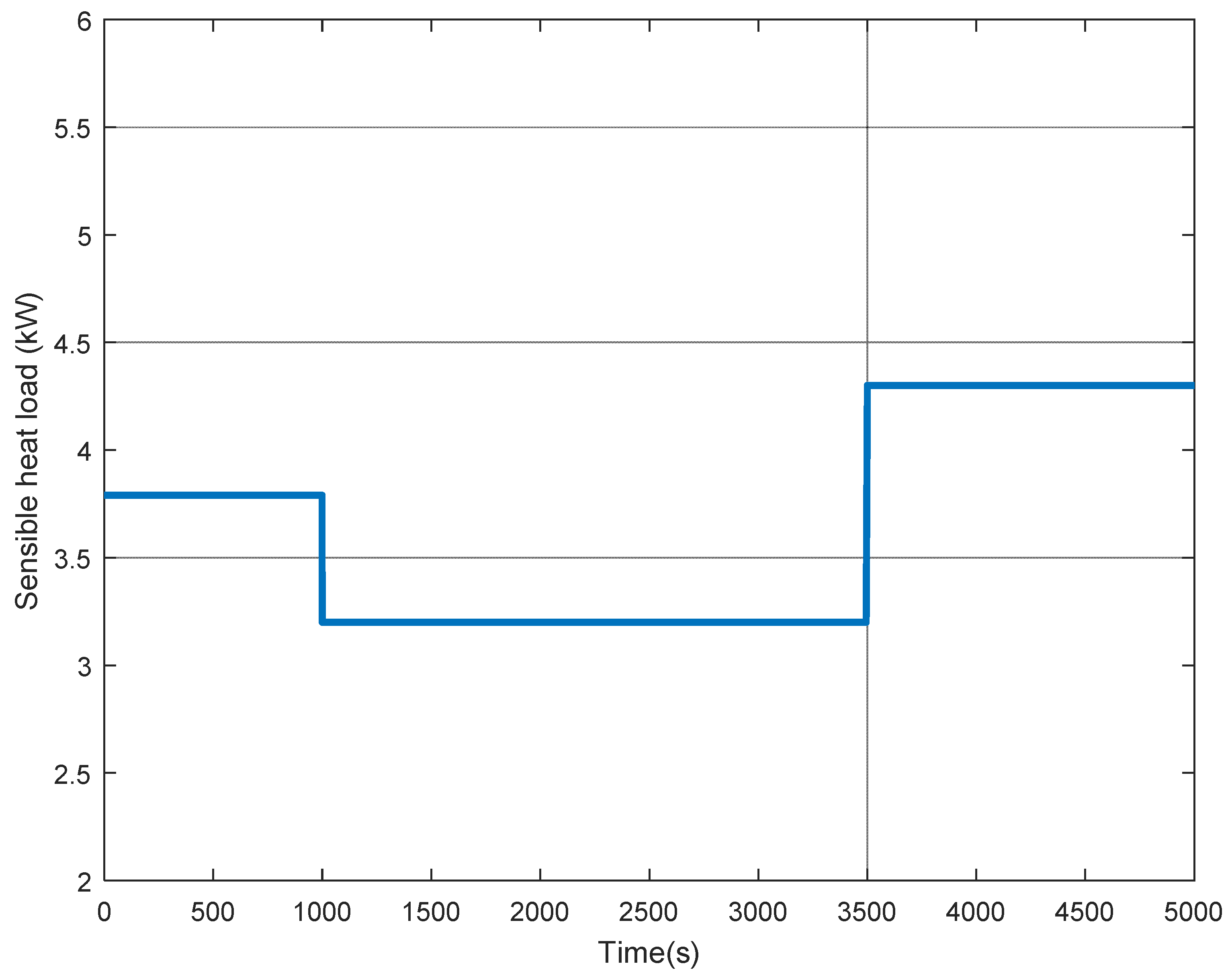
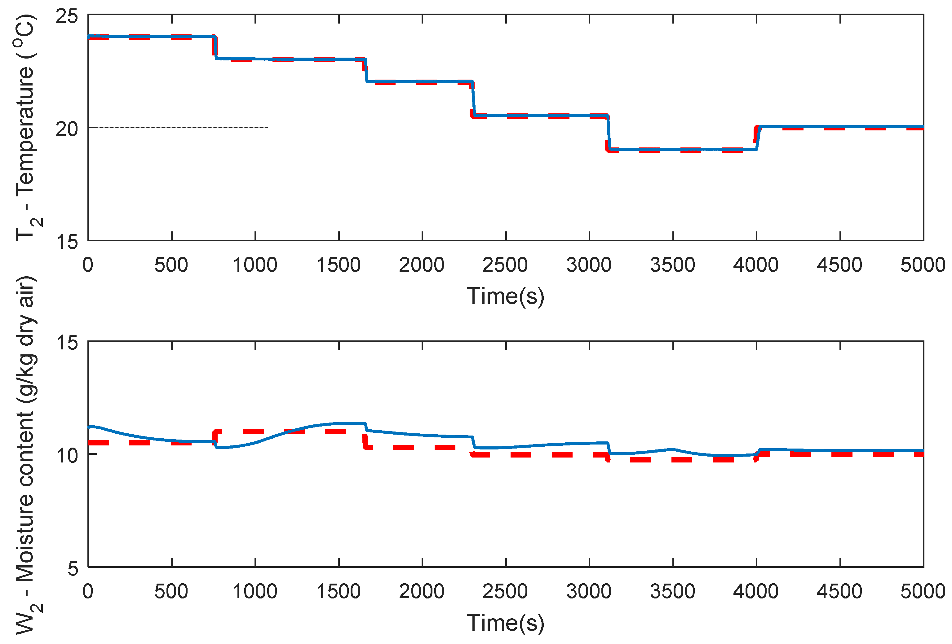
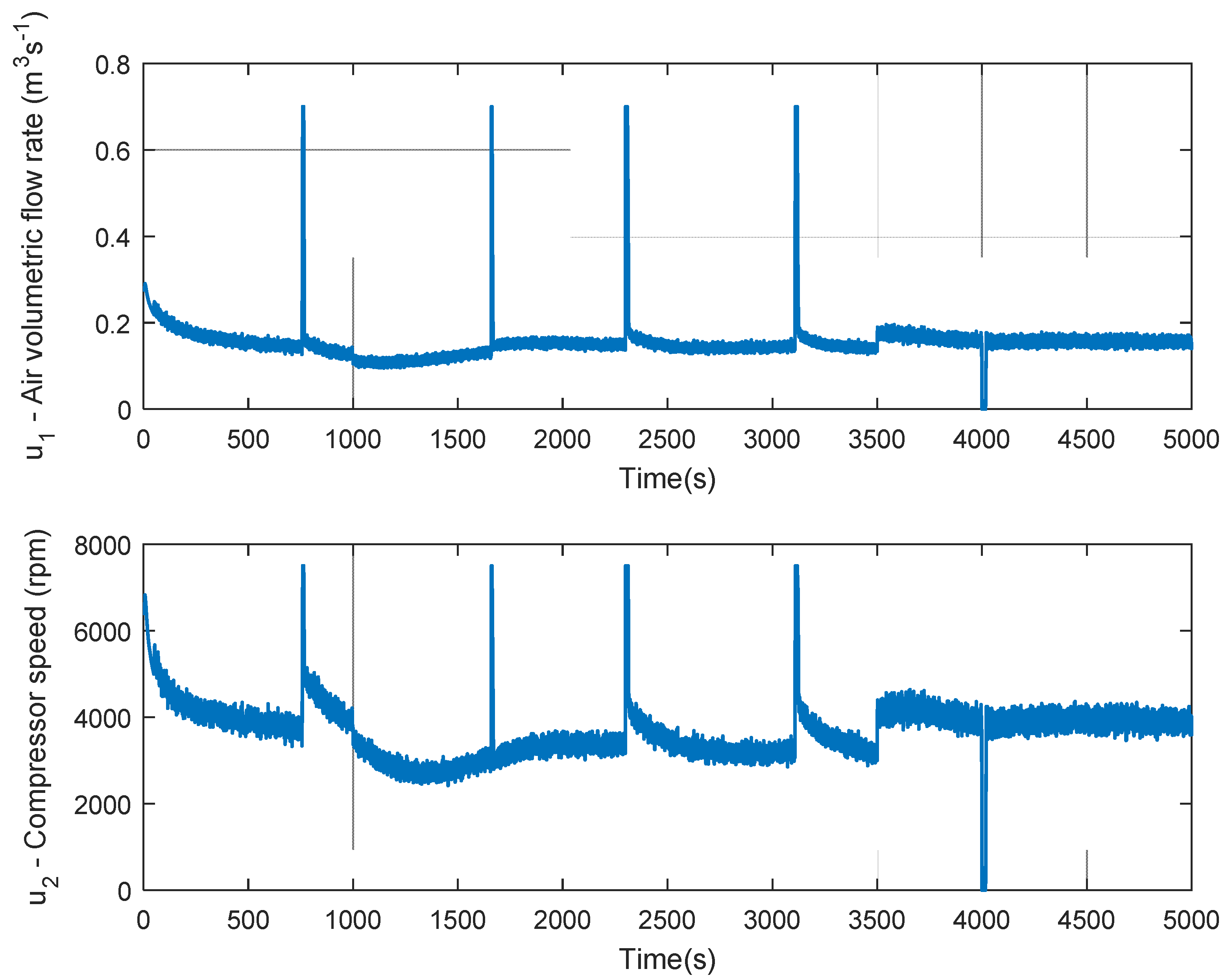
3.2. Controllability Simulation Test

A test to examine the control scheme performance is conducted. The reference trajectories are stepped waves for temperature and moisture, using the experimental VS DX A/C system model, proposed neural identifier and developed controller. The result of the trajectory tracking performance for the moisture content of air-conditioned space and the air temperature in the conditioned space, in presence of a disturbance simulated by a uniform random signal, is presented in Figure 3. The disturbance is a random variation of a model parameter, thus simulating an internal variation in the system. By applying the inverse optimal control, the obtained control signals are portrayed in Figure 4. Additionally, Figure 4 shows fan and compressor efficient operation, which contributes to reduced energy consumption.

Figure 3. Tracking performance of VS DX A/C system with internal disturbances.

Figure 4. Control signals for tracking performance of VS DX A/C system with internal disturbances.

Trajectory tracking with disturbances test has operation conditions close to reality. As seen in Figure 3, humidity and indoor air temperature settings were initially set at 10.5 g kg⁻¹ for W₂ and 24 °C for T₂. First, at 760 s, humidity and indoor air temperature settings were changed to 11 g kg⁻¹ for W₂ and 23 °C for T₂. Next, at 1660 s, humidity and indoor air temperature settings were changed to 10.25 g kg⁻¹ for W₂ and 22 °C for T₂. At 2300 s, humidity and indoor air temperature settings were changed to 10 g kg⁻¹ for W₂ and 21.5 °C for T₂. At 3110 s, humidity and indoor air temperature settings were changed to 9.75 g kg⁻¹ for W₂ and 19 °C for T₂. Finally, at 4000 s, humidity and indoor air temperature settings were changed to 10 g kg⁻¹ for W₂ and 20 °C for T₂.

Finally, a variation of the sensible heat load is added as an external disturbance in a new test, as shown in Figure 5.

Figure 5. Variation of sensible heat load in the conditioned space.

Figure 6 shows the trajectory tracking considering internal and external disturbances. The control signals are displayed in Figure 7.

Figure 6. Tracking performance of VS DX A/C system with internal and external disturbances.

Figure 7. Control signals for tracking performance of VS DX A/C system with internal and external disturbances.

Again, Figure 7 shows an efficient operation due to the performance of the control signals, achieving reduced energy consumption.

There is a continuous search for alternatives that reduce the energy consumption of air conditioning systems since they are equipment commonly used from home, to schools, to offices, to department stores and to large companies. In most countries, the existence of air conditioning systems that do not have a variable speed compressor is extensive, increasing electrical energy consumption. However, the updating of this equipment is taking place gradually. Hence the importance of developing this type of work. The results obtained are comparable with [12], where a multivariable controller was designed, getting a small range of operation for the A/C system. Reference [14] proposes an ANN/fuzzy logic controller to control both temperature and humidity of an A/C system.

4. Conclusions

In this paper, the A/C system model utilized was taken from a VS DX A/C system, commonly used in homes, offices, classrooms and even small to medium-sized businesses. The conditions under which the model was obtained have been mentioned in the methodology. However, when using NN any condition not considered in the analysis is absorbed by the neural model. On the other hand, the paper presents trajectory tracking using neural inverse optimal control for nonlinear systems and is inverse optimal in the sense that, a posteriori, minimizes a meaningful cost functional achieving reduced energy consumption. Using an unscented Kalman filter, the neural network training is performed online. The proposed identification and control scheme by means of the simulation results shows its effectiveness and robustness. Therefore, this research shows a novel scheme exposed to a wider temperature and humidity range and a more significant number of their variations in the desired references, presenting a more efficient performance. In addition, the control signals that result from the proposed control scheme show reduced energy consumption. This work may have future research that will further reduce this energy consumption by implementing other novel control algorithms, which establish new solution alternatives.

References

- Chen, W.; Chan, M.; Deng, S.; Yan, H.; Weng, W. A direct expansion based enhanced dehumidification air conditioning system for improved year-round indoor humidity control in hot and humid climates. Build. Environ. 2018, 139, 95–109. [Google Scholar] [CrossRef]
- Chen, W.; Chan, M.; Weng, W.; Yan, H.; Deng, S. An experimental study on the operational characteristics of a direct expansion based enhanced dehumidification air conditioning system. Appl. Energy 2018, 225, 922–933. [Google Scholar] [CrossRef]
- Zhang, H.; Yoshino, H. Analysis of indoor humidity environment in Chinese residential buildings. Build. Environ. 2010, 45, 2132–2140. [Google Scholar] [CrossRef]
- Chen, W.; Chan, M.; Weng, W.; Yan, H.; Deng, S. Development of a steady-state physical-based mathematical model for a direct expansion based enhanced dehumidification air conditioning system. Int. J. Refrig. 2018, 91, 55–68. [Google Scholar] [CrossRef]
- Bordrick, J.; Gilbride, T.L. Focusing on Buyer’s Needs: DOE’s Engineering Technology Program. Energy Eng. 2002, 99, 18–37. [Google Scholar] [CrossRef]
- Zhang, G.Q. China HVACR annual volume II business. Chin. Constr. Ind. Press Beijing 2002, 2, 44–45. [Google Scholar]
- Kang, C.-S.; Hyun, C.-H.; Park, M. Fuzzy logic-based advanced on–off control for thermal comfort in residential buildings. Appl. Energy 2015, 155, 270–283. [Google Scholar] [CrossRef]
- Toftum, J.; Fanger, P.O. Air humidity requirements for human comfort. ASHRAE Trans. 1999, 105, 641–647. [Google Scholar]
- Krakow, K.I.; Lin, S.; Zeng, Z.-S. Temperature and humidity control during cooling and dehumidifying by compressor and evaporator fan speed variation. ASHRAE Trans. 1995, 101, 292–304. [Google Scholar]
- Diaz-Mendez, S.E.; Patiño-Carachure, C.; Herrera-Castillo, J.A. Reducing the energy consumption of an earth–air heat exchanger with a PID control system. Energy Convers. Manag. 2014, 77, 1–6. [Google Scholar] [CrossRef]
- Li, Z.; Deng, S. A DDC-based capacity controller of a direct expansion (DX) air conditioning (A/C) unit for simultaneous indoor air temperature and humidity control–Part I: Control algorithms and preliminary controllability tests. Int. J. Refrig. 2007, 30, 113–123. [Google Scholar] [CrossRef]
- Qi, Q.; Deng, S. Multivariable control of indoor air temperature and humidity in a direct expansion (DX) air conditioning (A/C) system. Build. Environ. 2009, 44, 1659–1667. [Google Scholar] [CrossRef]
- Li, N.; Xia, L.; Shiming, D.; Xu, X.; Chan, M.Y. Dynamic modeling and control of a direct expansion air conditioning system using artificial neural network. Appl. Energy 2012, 91, 290–300. [Google Scholar] [CrossRef]
- Li, Z.; Xu, X.; Deng, S.; Pan, D. A novel neural network aided fuzzy logic controller for a variable speed (VS) direct expansion (DX) air conditioning (A/C) system. Appl. Therm. Eng. 2015, 78, 9–23. [Google Scholar] [CrossRef]
- Xia, Y.; Yan, H.; Deng, S.; Chan, M.-Y. A new capacity controller for a direct expansion air conditioning system for operational safety and efficiency. Build. Serv. Eng. Res. Technol. 2018, 39, 21–37. [Google Scholar] [CrossRef]
- Diaz, S.E.; Sierra, J.M.T.; Herrera, J.A. The use of earth–air heat exchanger and fuzzy logic control can reduce energy consumption and environmental concerns even more. Energy Build. 2013, 65, 458–463. [Google Scholar] [CrossRef]
- Garces-Jimenez, A.; Gomez-Pulido, J.-M.; Gallego-Salvador, N.; Garcia-Tejedor, A.-J. Genetic and Swarm Algorithms for Optimizing the Control of Building HVAC Systems Using Real Data: A Comparative Study. Mathematics 2021, 9, 2181. [Google Scholar] [CrossRef]
- Adegbenro, A.; Short, M.; Angione, C. An Integrated Approach to Adaptive Control and Supervisory Optimisation of HVAC Control Systems for Demand Response Applications. Energies 2021, 14, 2078. [Google Scholar] [CrossRef]
- Jajarmi, A.; Pariz, N.; Effati, S.; Kamyad, A.V. Infinite horizon optimal control for nonlinear interconnected large-scale dynamical systems with an application to optimal attitude control. Asian J. Control 2012, 14, 1239–1250. [Google Scholar] [CrossRef]
- Baleanu, D.; Zibaei, S.; Namjoo, M.; Jajarmi, A. A nonstandard finite difference scheme for the modeling and nonidentical synchronization of a novel fractional chaotic system. Adv. Differ. Equ. 2021, 2021, 308. [Google Scholar] [CrossRef]
- Jajarmi, A.; Baleanu, D.; Zarghami Vahid, K.; Mobayen, S. A general fractional formulation and tracking control for immunogenic tumor dynamics. Math. Methods Appl. Sci. 2022, 45, 667–680. [Google Scholar] [CrossRef]
- Willis, M.J.; Montague, G.A.; Di Massimo, C.; Tham, M.T.; Morris, A.J. Artificial neural networks in process estimation and control. Automatica 1992, 28, 1181–1187. [Google Scholar] [CrossRef]
- Trebatický, P. Recurrent neural network training with the extended kalman filter. In Proceedings of the Student Research Conf. in Informatics and Information Technologies, Bratislava, Slovakia, 27 April 2005; pp. 57–64. [Google Scholar]
- Feldkamp, L.A.; Prokhorov, D.V.; Feldkamp, T.M. Simple and conditioned adaptive behavior from Kalman filter trained recurrent networks. Neural Netw. 2003, 16, 683–689. [Google Scholar] [CrossRef]
- Alanis, A.Y.; Sanchez, E.N.; Loukianov, A.G.; Perez-Cisneros, M.A. Real-time discrete neural block control using sliding modes for electric induction motors. IEEE Trans. Control Syst. Technol. 2010, 18, 11–21. [Google Scholar] [CrossRef]
- Leung, C.-S.; Chan, L.-W. Dual extended Kalman filtering in recurrent neural networks. Neural Netw. 2003, 16, 223–239. [Google Scholar] [CrossRef]
- Haykin, S. Kalman filters. In Kalman Filtering and Neural Networks; Haykin, S., Ed.; John Wiley & Sons, Inc.: New York, NY, USA, 2001; pp. 1–21. ISBN 978-0-471-36998-1. [Google Scholar]
- Julier, S.J.; Uhlmann, J.K. New extension of the Kalman filter to nonlinear systems. In Proceedings of the Signal Processing, Sensor Fusion, and Target Recognition VI, Orlando, FL, USA, 28 July 1997; pp. 182–193. [Google Scholar]
- Trebatický, P.; Pospíchal, J. Neural Network Training with Extended Kalman Filter Using Graphics Processing Unit. In Artificial Neural Networks-ICANN 2008; Springer: Berlin/Heidelberg, Germany, 2008; pp. 198–207. [Google Scholar]
- Kirk, D.E. Optimal Control Theory: An Introduction, 2nd ed.; Dover Publication, Inc.: Mineola, NY, USA, 2004. [Google Scholar]
- Krstic, M.; Kanellakopoulos, I.; Kokotovic, P.V. Nonlinear and Adaptive Control Design; John Wiley and Sons: New York, NY, USA, 1995. [Google Scholar]
- Do, K.D.; Jiang, Z.P.; Pan, J. Simultaneous Tracking and Stabilization of Mobile Robots: An Adaptive Approach. IEEE Trans. Automat. Contr. 2004, 49, 1147–1152. [Google Scholar] [CrossRef]
- Hernandez-Mejia, G.; Alanis, A.Y.; Hernandez-Vargas, E.A. Neural inverse optimal control for discrete-time impulsive systems. Neurocomputing 2018, 314, 101–108. [Google Scholar] [CrossRef]
- Ruiz-Cruz, R.; Sanchez, E.N.; Loukianov, A.G.; Ruz-Hernandez, J.A. Real-Time Neural Inverse Optimal Control for a Wind Generator. IEEE Trans. Sustain. Energy 2019, 10, 1172–1183. [Google Scholar] [CrossRef]
- Quintero-Manríquez, E.; Sanchez, E.N.; Antonio-Toledo, M.E.; Muñoz, F. Neural control of an induction motor with regenerative braking as electric vehicle architecture. Eng. Appl. Artif. Intell. 2021, 104, 104275. [Google Scholar] [CrossRef]
- Qi, Q.; Deng, S. Multivariable control-oriented modeling of a direct expansion (DX) air conditioning (A/C) system. Int. J. Refrig. 2008, 31, 841–849. [Google Scholar] [CrossRef]
- Narendra, K.S.; Parthasarathy, K. Identification and control of dynamical systems using neural networks. IEEE Trans. Neural Netw. 1990, 1, 4–27. [Google Scholar] [CrossRef] [PubMed]
- Rovithakis, G.A.; Christodoulou, M.A. Adaptive Control with Recurrent High-Order Neural Networks; Advances in Industrial Control; Springer: Berlin, Germany, 2000; ISBN 978-1-4471-1201-3. [Google Scholar]
- Haddad, W.M.; Chellaboina, V.-S.; Fausz, J.L.; Abdallah, C. Optimal discrete-time control for non-linear cascade systems. J. Frankl. Inst. 1998, 335, 827–839. [Google Scholar] [CrossRef][Green Version]
- Prokhorov, D.V. Kalman Filter Training of Neural Networks: Methodology and Applications. In Proceedings of the International Joint Conference on Neural Networks, IJCNN2004 Tutorials, Budapest, Hungary, 25–29 July 2004. [Google Scholar]
- Rhudy, M.; Gu, Y.; Napolitano, M.R. An Analytical Approach for Comparing Linearization Methods in EKF and UKF. Int. J. Adv. Robot. Syst. 2013, 10, 208. [Google Scholar] [CrossRef]
- Wan, E.A.; van der Merwe, R. The Unscented Kalman Filter. In Kalman Filtering and Neural Networks; Haykin, S., Ed.; John Wiley & Sons, Inc.: New York, NY, USA, 2001; pp. 221–280. ISBN 978-0-471-36998-1. [Google Scholar]
- Rhudy, M.; Gu, Y.; Gross, J.; Napolitano, M.R. Evaluation of Matrix Square Root Operations for UKF within a UAV GPS/INS Sensor Fusion Application. Int. J. Navig. Obs. 2011, 2011, 1–11. [Google Scholar] [CrossRef]
- Van der Merwe, R.; Wan, E.A. The square-root unscented Kalman filter for state and parameter-estimation. In Proceedings of the International Conference on Acoustics, Speech, and Signal Processing, Salt Lake City, UT, USA, 7–11 May 2001; Volume 6, pp. 3461–3464. [Google Scholar]
- Başar, T.; Olsder, G.J. Dynamic Noncooperative Game Theory, 2nd ed.; Academic Press: New York, NY, USA, 1995; ISBN 978-0-89871-429-6. [Google Scholar]
- Lewis, F.L.; Syrmos, V.L. Optimal Control, 2nd ed.; John Wiley & Sons: New York, NY, USA, 1995. [Google Scholar]
- Al-Tamimi, A.; Lewis, F.L.; Abu-Khalaf, M. Discrete-Time Nonlinear HJB Solution Using Approximate Dynamic Programming: Convergence Proof. IEEE Trans. Syst. Man Cybern. Part B 2008, 38, 943–949. [Google Scholar] [CrossRef] [PubMed]
- Ohsawa, T.; Bloch, A.M.; Leok, M. Discrete Hamilton-Jacobi theory and discrete optimal control. In Proceedings of the 49th IEEE Conference on Decision and Control (CDC), Atlanta, GA, USA, 15–17 December 2010; pp. 5438–5443. [Google Scholar]
Publisher’s Note: MDPI stays neutral with regard to jurisdictional claims in published maps and institutional affiliations. |
© 2022 by the authors. Licensee MDPI, Basel, Switzerland. This article is an open access article distributed under the terms and conditions of the Creative Commons Attribution (CC BY) license (https://creativecommons.org/licenses/by/4.0/).