Runge-Kutta-Nyström Pairs of Orders 8(6) with Coefficients Trained to Perform Best on Classical Orbits

Abstract

In this study, we consider eight stages per step family of explicit Runge-Kutta-Nyström pairs of orders eight and six. The pairs from this family effectively use eight stages for each step. The coefficients provided by such a method are much less than the number of non linear order conditions required to be solved. Thus, we traditionally apply various simplified assumptions in order to address this drawback. The assumptions taken in the family we consider here deliver a subsystem where all the coefficients are evaluated successively and explicitly with respect to five free parameters. We train (adjust) these free parameters in order to derive a certain pair that outperforms other similar pairs of orders $8(6)$ in Keplerian type orbits, e.g., Kepler, perturbed Kepler, Arenstorf orbit, or Pleiades. Differential evolution technique is used for the training. The pair that we finally present offers about an additional digit of accuracy in a variety of orbits.

1. Introduction

The initial value problem of special form

$${\psi }^{″}=\phi (x,\psi ),\psi (x_0)={\psi }_0,{\psi }^{\prime }(x_0)={\displaystyle {\psi }_0^{\prime }}$$

(1)

where $\phi :\mathbb{R}\times {\mathbb{R}}^m\to {\mathbb{R}}^m,$ and $({\psi }_0,{\displaystyle {\psi }_0^{\prime }})\in {\mathbb{R}}^{2m},$ is considered here.

We approximate the solution of (1) at a set of discrete points $\left(x_n,{\psi }_n,{\displaystyle {\psi }_n^{\prime }}\right)$ with an explicit Runge-Kutta-Nyström (RKN) pair of orders $p(q),$ $p>q$. This method has the form

$${\phi }_i=\phi (x_n+{\gamma }_i{h}_n,{\psi }_n+{\gamma }_i{h}_n{\displaystyle {\psi }_n^{\prime }}+{\displaystyle h_n^2}{\displaystyle \sum _{j=1}^s}{\alpha }_{ij}{\phi }_j),i=1,2,\cdots ,s$$

$$\begin{array}{cc}{\psi }_{n+1}={\psi }_n+h_n{\displaystyle {\psi }_n^{\prime }}+{\displaystyle h_n^2}{\displaystyle {\sum }_{i=1}^s}{\beta }_i{\phi }_i,\hfill & {\widehat{\psi }}_{n+1}={\psi }_n+h_n{\displaystyle {\psi }_n^{\prime }}+{\displaystyle h_n^2}{\displaystyle {\sum }_{i=1}^s}{\widehat{\beta }}_i{\phi }_i,\hfill \\ {\displaystyle {\psi }_{n+1}^{\prime }}={\displaystyle {\psi }_n^{\prime }}+h_n{\displaystyle {\sum }_{i=1}^s}{\displaystyle {\beta }_i^{\prime }}{\phi }_i,\hfill & {\displaystyle {\widehat{\psi }}_{n+1}^{\prime }}={\displaystyle {\psi }_n^{\prime }}+h_n{\displaystyle {\sum }_{i=1}^s}{\displaystyle {\widehat{\beta }}_i^{\prime }}{\phi }_i,\hfill \end{array}$$

with $h_n=x_{n+1}-x_n,$ while the number of the stages of the method is s. The solution is propagated by the higher order approximations ${\psi }_n,{\displaystyle {\psi }_n^{\prime }}$. In consequence, $\widehat{\beta }$ and ${\widehat{\beta }}^{\prime }$ correspond to the lower order method.

Some norm of the vector estimating the error

$${ϵ}_n=max(\parallel {\displaystyle h_n^2}{\displaystyle \sum _{i=1}^s}({\beta }_i-{\widehat{\beta }}_i){\phi }_i\parallel ,\parallel h_n{\displaystyle \sum _{i=1}^s}({\displaystyle {\beta }_i^{\prime }}-{\displaystyle {\widehat{\beta }}_i^{\prime }}){\phi }_i)\parallel ,$$

is used in comparison with the requested tolerance $TOL$, for step-size control algorithm

$$h_{n+1}=0.9·h_n·{\left(\frac{TOL}{{\displaystyle h_n^{p-q+1}}·{ϵ}_n}\right)}^{1/p}.$$

This formula is used even if $TOL<h^{p-q+1}·{ϵ}_n$, but then $h_{n+1}$ is actually a new smaller version of $h_n$. For extended details in the issue, see [1].

All the coefficients can be formulated using the Butcher tableau [2,3]. So the method takes the form

$$\begin{array}{cc}\gamma & A\\ & \begin{array}{cc}\beta & \widehat{\beta }\\ {\beta }^{\prime }& {\widehat{\beta }}^{\prime }\end{array}\end{array}$$

with $A\in {\mathbb{R}}^{s\times s},$${\beta }^{\mathrm{T}},{\widehat{\beta }}^{\mathrm{T}},{\beta \prime }^{\mathrm{T}},{\widehat{\beta }}^{\mathrm{T}},\gamma \in {\mathbb{R}}^s.$ Here, matrix A is strictly lower triangular since the methods considered are explicit. By this we mean that the function evaluations (i.e., ${\varphi }_i$’s) are calculated directly and successively. On the contrary, when the method is implicit we have to solve non linear equations for evaluating the stages, which increases the computation time. Implicit methods are used when the problems are stiff [4]. The problems we are dealing with in the following do not fall into the latter category [5].

Here we are interested in studying nine stages (i.e., $s=9$), FSAL (First stage As Last) pair of orders eight and six (i.e., $p=8$ and $q=6$). This method spends only eight stages per step since the last stage is used again as the first stage in the next step. Thus, the coefficients in the ninth stage coincide with $\beta$, i.e., $a_{9j}={\beta }_j$ for $j=1,2,\cdots ,8$.

2. The Dormand-El Mikkawy-Prince Family of Runge-Kutta-Nyström Pairs of Orders 8(6)

This family is used for the derivation of the famous DEP8(6) pair presented in [6]. Further investigation is given in [1]. Thus, we may deploy here the algorithm for the derivation of the parameters of the pair with respect to the free terms ${\gamma }_4,{\gamma }_5,{\gamma }_6,{\gamma }_7$ and ${\widehat{\beta }}_9$.

Initially, set ${\gamma }_8={\gamma }_9=1$. All the coefficients not presented below are zero, e.g., ${\displaystyle {\beta }_2^{\prime }}=0$.

$${\gamma }_3=\frac{\left\{\begin{array}{c}15-20{\gamma }_4-20{\gamma }_5+28{\gamma }_4{\gamma }_5-20{\gamma }_6+28{\gamma }_4{\gamma }_6+28{\gamma }_5{\gamma }_6-42{\gamma }_4{\gamma }_5{\gamma }_6\\ -20{\gamma }_7+28{\gamma }_4{\gamma }_7+28{\gamma }_5{\gamma }_7-42{\gamma }_4{\gamma }_5{\gamma }_7+28{\gamma }_6{\gamma }_7\\ -42{\gamma }_4{\gamma }_6{\gamma }_7-42{\gamma }_5{\gamma }_6{\gamma }_7+70{\gamma }_4{\gamma }_5{\gamma }_6{\gamma }_7\end{array}\right\}}{\left\{\begin{array}{c}2(10-14{\gamma }_4-14{\gamma }_5+21{\gamma }_4{\gamma }_5-14{\gamma }_6+21{\gamma }_4{\gamma }_6+21{\gamma }_5{\gamma }_6\\ -35{\gamma }_4{\gamma }_5{\gamma }_6-14{\gamma }_7+21{\gamma }_4{\gamma }_7+21{\gamma }_5{\gamma }_7-35{\gamma }_4{\gamma }_5{\gamma }_7\\ +21{\gamma }_6{\gamma }_7-35{\gamma }_4{\gamma }_6{\gamma }_7-35{\gamma }_5{\gamma }_6{\gamma }_7+70{\gamma }_4{\gamma }_5{\gamma }_6{\gamma }_7)\end{array}\right\}},$$

$${\gamma }_2=\frac{1}{2}{\gamma }_3.$$

Then solve

$$b^{\prime }·e=1,b^{\prime }·\gamma =\frac{1}{2},b^{\prime }·{\gamma }^2=\frac{1}{3},b^{\prime }·{\gamma }^3=\frac{1}{4},b^{\prime }·{\gamma }^4=\frac{1}{5},b^{\prime }·{\gamma }^5=\frac{1}{6},b^{\prime }·{\gamma }^6=\frac{1}{7}$$

for ${\displaystyle {\beta }_1^{\prime }},{\displaystyle {\beta }_3^{\prime }},{\displaystyle {\beta }_4^{\prime }},{\displaystyle {\beta }_5^{\prime }},{\displaystyle {\beta }_6^{\prime }},{\displaystyle {\beta }_7^{\prime }}$ and ${\displaystyle {\beta }_8^{\prime }}$.

In these equations, “∗” is to be understood as a component-wise multiplication among vectors and has the lowest priority after all other operations. Also,

$${\gamma }^2=\gamma \ast \gamma ,{\gamma }^3={\gamma }^2\ast \gamma ,\mathrm{etc}.$$

This latter operation (“raising” a vector to a power) has highest priority and is evaluated before the dot products and “∗”.

Set ${\beta }_i={\beta }_i\left(1-{\gamma }_i\right),$ for $i=1,2,\cdots ,8.$

In consequence from FSAL property follows that $a_{9i}={\beta }_i,i=1,2,\cdots ,8.$

Continue evaluating successively

$$a_{32}=\frac{{\displaystyle {\gamma }_3^2}}{6{\gamma }_2},$$

$$a_{42}=\frac{{\displaystyle {\gamma }_4^3}(-2{\gamma }_3+{\gamma }_4)}{12{\gamma }_2({\gamma }_2-{\gamma }_3)},$$

$$a_{43}=\frac{{\displaystyle {\gamma }_4^3}(-2{\gamma }_2+{\gamma }_4)}{12{\gamma }_3(-{\gamma }_2+{\gamma }_3)},$$

$$a_{65}=\frac{9-20{\gamma }_3-20{\gamma }_4+56{\gamma }_3{\gamma }_4-12{\gamma }_7+28{\gamma }_3{\gamma }_7+28{\gamma }_4{\gamma }_7-84{\gamma }_3{\gamma }_4{\gamma }_7}{10,080({\gamma }_3-{\gamma }_5){\gamma }_5(-{\gamma }_4+{\gamma }_5)(-1+{\gamma }_6)({\gamma }_6-{\gamma }_7)db6},$$

$$a_{75}=\frac{\left\{\begin{array}{c}-9{\gamma }_5+20{\gamma }_3{\gamma }_5+20{\gamma }_4{\gamma }_5-56{\gamma }_3{\gamma }_4{\gamma }_5+15{\gamma }_6-32{\gamma }_3{\gamma }_6-32{\gamma }_4{\gamma }_6+84{\gamma }_3{\gamma }_4{\gamma }_6\\ -12{\displaystyle {\gamma }_6^2}+28{\gamma }_3{\displaystyle {\gamma }_6^2}+28{\gamma }_4{\displaystyle {\gamma }_6^2}-84{\gamma }_3{\gamma }_4{\displaystyle {\gamma }_6^2}-6{\gamma }_7+12{\gamma }_3{\gamma }_7+12{\gamma }_4{\gamma }_7\\ -28{\gamma }_3{\gamma }_4{\gamma }_7+12{\gamma }_5{\gamma }_7-28{\gamma }_3{\gamma }_5{\gamma }_7-28{\gamma }_4{\gamma }_5{\gamma }_7+84{\gamma }_3{\gamma }_4{\gamma }_5{\gamma }_7\end{array}\right\}}{10,080({\gamma }_3-{\gamma }_5){\gamma }_5(-{\gamma }_4+{\gamma }_5)({\gamma }_5-{\gamma }_6)({\gamma }_6-{\gamma }_7)(-1+{\gamma }_7){\displaystyle {\beta }_7^{\prime }}},$$

$$a_{76}=\frac{3-6{\gamma }_3-6{\gamma }_4+14{\gamma }_3{\gamma }_4-6{\gamma }_5+14{\gamma }_3{\gamma }_5+14{\gamma }_4{\gamma }_5-42{\gamma }_3{\gamma }_4{\gamma }_5}{5040({\gamma }_3-{\gamma }_6){\gamma }_6(-{\gamma }_4+{\gamma }_6)(-{\gamma }_5+{\gamma }_6)(-1+{\gamma }_7){\displaystyle {\beta }_7^{\prime }})},$$

$$a_{85}=-\frac{-{\displaystyle {\beta }_5^{\prime }}+2{\gamma }_5{\displaystyle {\beta }_5^{\prime }}-{\displaystyle {\gamma }_5^2}{\displaystyle {\beta }_5^{\prime }}+2a_{65}{\displaystyle {\beta }_6^{\prime }}+2a_{75}{\displaystyle {\beta }_7^{\prime }}}{2{\displaystyle {\beta }_8^{\prime }}},$$

$$a_{86}=\frac{-{\displaystyle {\beta }_6^{\prime }}+2{\gamma }_6{\displaystyle {\beta }_6^{\prime }}-{\displaystyle {\gamma }_6^2}{\displaystyle {\beta }_6^{\prime }}+2a_{76}{\displaystyle {\beta }_7^{\prime }}}{2{\displaystyle {\beta }_8^{\prime }}},$$

$$a_{87}=\frac{{\displaystyle {\beta }_7^{\prime }}-2{\gamma }_7{\displaystyle {\beta }_7^{\prime }}+{\displaystyle {\gamma }_7^2}{\displaystyle {\beta }_7^{\prime }}}{2{\displaystyle {\beta }_8^{\prime }}}.$$

Then solve simultaneously

$${\widehat{\beta }}^{\prime }·e=1,{\widehat{\beta }}^{\prime }·\gamma =\frac{1}{2},{\widehat{\beta }}^{\prime }·{\gamma }^2=\frac{1}{3},{\widehat{\beta }}^{\prime }·{\gamma }^3=\frac{1}{4},{\widehat{\beta }}^{\prime }·{\gamma }^4=\frac{1}{5},{\widehat{\beta }}^{\prime }·{\gamma }^5=\frac{1}{6}$$

and

$$\begin{array}{c}\widehat{\beta }·A·\left(\Gamma -{\gamma }_{3}I\right)·\left(\Gamma -{\gamma }_{4}I\right)·\gamma -{\gamma }_2\left({\gamma }_2-{\gamma }_3\right)\left({\gamma }_2-{\gamma }_4\right){\left({\widehat{\beta }}^{\prime }·A\right)}_2=\hfill \\ ={\displaystyle {\int }_{x=0}^{x=1}}{\displaystyle {\int }_{x=0}^{x=x}}{\displaystyle {\int }_{x=0}^{x=x}}\left(x-{\gamma }_3\right)\left(x-{\gamma }_4\right)xdxdxdx\hfill \end{array}$$

for ${\displaystyle {\widehat{\beta }}_1^{\prime }},{\displaystyle {\widehat{\beta }}_3^{\prime }},{\displaystyle {\widehat{\beta }}_4^{\prime }},{\displaystyle {\widehat{\beta }}_5^{\prime }},{\displaystyle {\widehat{\beta }}_6^{\prime }},{\displaystyle {\widehat{b}}_7^{\prime }}$ and ${\displaystyle {\widehat{\beta }}_8^{\prime }},$ assuming that $\Gamma =\mathrm{diag}(\gamma )$.

Also set ${\widehat{\beta }}_i={\displaystyle {\widehat{\beta }}_i^{\prime }}\left(1-{\gamma }_i\right),$ for $i=1,2,\cdots ,8.$

Proceed solving

$${\left(b^{\prime }·A\right)}_2={\left(b^{\prime }·\left(\gamma \ast A\right)\right)}_2={\left(b^{\prime }·\left({\gamma }^2\ast A\right)\right)}_2={\left({\widehat{\beta }}^{\prime }·A\right)}_2=0$$

for $a_{52},a_{62},a_{72}$ and $a_{82}.$

After this, evaluate successively

$$\begin{array}{ccc}\hfill a_{53}& =& \frac{12a_{52}{\displaystyle {\gamma }_2^2}+12a_{52}{\gamma }_2{\gamma }_4-2{\gamma }_4{\displaystyle {\gamma }_5^3}+{\displaystyle {\gamma }_5^4}}{12{\gamma }_3({\gamma }_3-{\gamma }_4)},\hfill \\ \hfill a_{54}& =& \frac{-12a_{52}{\displaystyle {\gamma }_2^2}+12a_{52}{\gamma }_2{\gamma }_3-2{\gamma }_3{\displaystyle {\gamma }_5^3}+{\displaystyle {\gamma }_5^4}}{12{\gamma }_4(-{\gamma }_3+{\gamma }_4))},\hfill \\ \hfill a_{63}& =& \frac{-12a_{62}{\displaystyle {\gamma }_2^2}+12a_{62}{\gamma }_2{\gamma }_4+12a_{65}{\gamma }_4{\gamma }_5-12a_{65}{\displaystyle {\gamma }_5^2}-2{\gamma }_4{\displaystyle {\gamma }_6^3}+{\displaystyle {\gamma }_6^4}}{12{\gamma }_3({\gamma }_3-{\gamma }_4)},\hfill \\ \hfill a_{64}& =& \frac{-12a_{62}{\displaystyle {\gamma }_2^2}+12a_{62}{\gamma }_2{\gamma }_3+12a_{65}{\gamma }_3{\gamma }_5-12a_{65}{\displaystyle {\gamma }_5^2}-2{\gamma }_3{\displaystyle {\gamma }_6^3}+{\displaystyle {\gamma }_6^4}}{12{\gamma }_4(-{\gamma }_3+{\gamma }_4)},\hfill \\ \hfill a_{73}& =& \frac{-12a_{72}{\displaystyle {\gamma }_2^2}+12a_{72}{\gamma }_2{\gamma }_4+12a_{75}{\gamma }_4{\gamma }_5-12a_{75}{\displaystyle {\gamma }_5^2}+12a_{76}{\gamma }_4{\gamma }_6-12a_{76}{\displaystyle {\gamma }_6^2}-2{\gamma }_4{\displaystyle {\gamma }_7^3}+{\displaystyle {\gamma }_7^4}}{12{\gamma }_3({\gamma }_3-{\gamma }_4)},\hfill \\ \hfill a_{74}& =& \frac{-12a_{72}{\displaystyle {\gamma }_2^2}+12a_{72}{\gamma }_2{\gamma }_3+12a_{75}{\gamma }_3{\gamma }_5-12a_{75}{\displaystyle {\gamma }_5^2}+12a_{76}{\gamma }_3{\gamma }_6-12a_{76}{\displaystyle {\gamma }_6^2}-2{\gamma }_3{\displaystyle {\gamma }_7^3}+{\displaystyle {\gamma }_7^4}}{12{\gamma }_4(-{\gamma }_3+{\gamma }_4)},\hfill \\ \hfill a_{83}& =& -\frac{-{\displaystyle {\beta }_3^{\prime }}+2{\gamma }_3{\displaystyle {\beta }_3^{\prime }}-{\displaystyle {\gamma }_3^2}{\displaystyle {\beta }_3^{\prime }}+2a_{43}{\displaystyle {\beta }_4^{\prime }}+2a_{53}{\displaystyle {\beta }_5^{\prime }}+2a_{63}{\displaystyle {\beta }_6^{\prime }}+2a_{73}{\displaystyle {\beta }_7^{\prime }}}{2{\displaystyle {\beta }_8^{\prime }}},\hfill \\ \hfill a_{84}& =& -\frac{-{\displaystyle {\beta }_4^{\prime }}+2{\gamma }_4{\displaystyle {\beta }_4^{\prime }}-{\displaystyle {\gamma }_4^2}{\displaystyle {\beta }_4^{\prime }}+2a_{54}{\displaystyle {\beta }_5^{\prime }}+2a_{64}{\displaystyle {\beta }_6^{\prime }}+2a_{74}{\displaystyle {\beta }_7^{\prime }}}{2{\displaystyle {\beta }_8^{\prime }}}.\hfill \end{array}$$

Conclude with

$$a_{i1}=\frac{1}{2}{\displaystyle {\gamma }_i^2}-{\displaystyle \sum _{j=2}^{i-1}}{a}_{i,j}.$$

Because the ninth stage is used as the first stage of the next step, even though $s=9$, the family wastes only eight stages each step.

The challenge now is how to choose the free parameters. The norm of the principal coefficients of the local truncation error is traditionally minimized, i.e., the coefficients of $h^8$ in the residual of Taylor error expansions corresponding to the 5th order formula of the underlying RK pair.

Since our concern here is to deal with Keplerian type orbits, we shall try another approach and train these free parameters in order for the resulting pair to perform best in our problems of interest.

3. Comparison of Outcomes from Various Pairs

Comparison of the results observed by various pairs is an interesting issue. It is of crucial importance in our present work. We thus deal with the Kepler problem. This has a form that follows

$$\begin{array}{c}{}^1{\psi }^{\prime }={}^3\psi ,\hfill \\ {}^2{\psi }^{\prime }={}^4\psi ,\hfill \\ {}^3{\psi }^{\prime }=-{\displaystyle \frac{{}^1\psi }{{\left(\sqrt{{{(}^1\psi )}^2+{{(}^2\psi )}^2}\right)}^3}},\hfill \\ {}^4{\psi }^{\prime }=-{\displaystyle \frac{{}^2\psi }{{\left(\sqrt{{{(}^1\psi )}^2+{{(}^2\psi )}^2}\right)}^3}},\hfill \end{array}$$

with $x\in [0,10\pi ]$, $\psi (0)={\left[1-\tau ,0,0,\sqrt{\frac{1+\tau }{1-\tau }}\right]}^T$ and the theoretical solution is [5]

$${}^1\psi (x)=cos(v)-\tau ,{}^2\psi (x)=sin(v)\sqrt{1-{\tau }^2}.$$

In the above, $v=\tau ·sin(v)+x$, $\tau$ is the eccentricity, and the left superscript denotes the components of $\psi$. We have to avoid confusion with ${\psi }_1={\left[{}^1{\psi }_1{,}^2{\psi }_1{,}^3{\psi }_1{,}^4{\psi }_1\right]}^T,$${\psi }_2={\left[{}^1{\psi }_2{,}^2{\psi }_2{,}^3{\psi }_2{,}^4{\psi }_2\right]}^T,{\psi }_3,\cdots$, that correspond to the vectors approximating the solution at $x_1,x_2,x_3,\cdots$.

When running DEP8(6) for $\tau =0.8$ and tolerances ${10}^{-5}$, ${10}^{-6},\cdots$, ${10}^{-11}$, we get the results summarized in Table 1. There we recorded the error observed at the end-point and the stages used by each pair.

Table 1. Outcomes of DEP8(6) on Kepler orbit for $\tau =0.8$.

Tolerance	Stages	End-Point Error
${10}^{-5}$	1089	$6.4\times {10}^{-4}$
${10}^{-6}$	1377	$2.7\times {10}^{-5}$
${10}^{-7}$	1769	$2.6\times {10}^{-7}$
${10}^{-8}$	2265	$1.3\times {10}^{-8}$
${10}^{-9}$	2889	$6.9\times {10}^{-8}$
${10}^{-10}$	3497	$4.0\times {10}^{-9}$
${10}^{-11}$	3785	$2.5\times {10}^{-10}$

Then, we try the PT8(6) pair given in [1] and get the results presented in Table 2.

Table 2. Outcomes of PT8(6) on Kepler orbit for $\tau =0.8$.

Tolerance	Stages	End-Point Error
${10}^{-5}$	1161	$5.0\times {10}^{-4}$
${10}^{-6}$	1457	$1.6\times {10}^{-6}$
${10}^{-7}$	1833	$4.5\times {10}^{-7}$
${10}^{-8}$	2361	$3.4\times {10}^{-8}$
${10}^{-9}$	3057	$3.7\times {10}^{-9}$
${10}^{-10}$	3729	$1.2\times {10}^{-9}$
${10}^{-11}$	3769	$2.4\times {10}^{-10}$

The question we raise now is regarding which pair delivers the better results. It is not clear from what can be seen in the tables. Thus, we use a technique similar to the one described in [5].

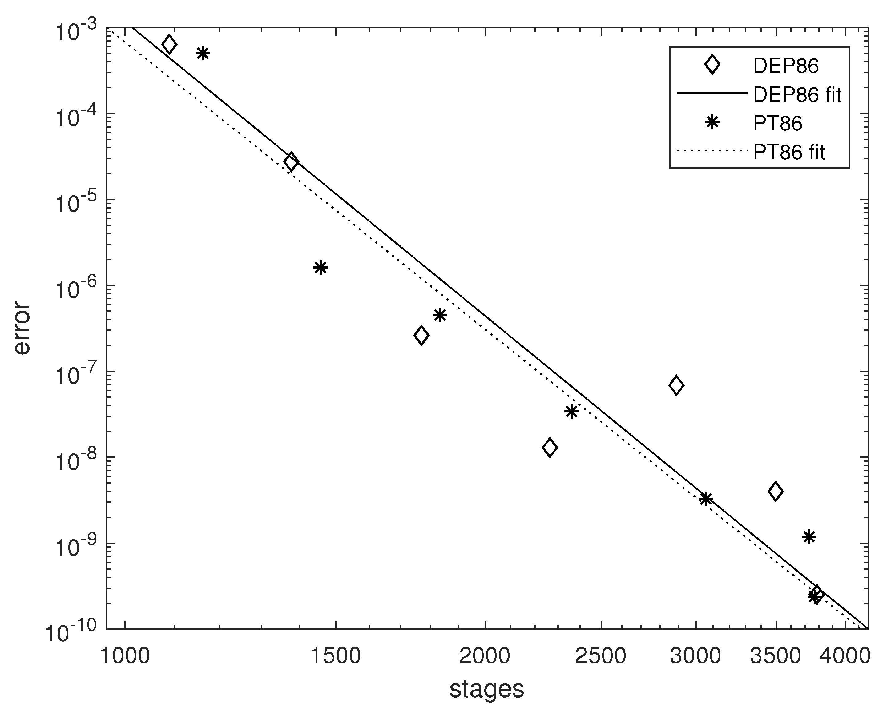
We form a linear least squares fit on the logarithms of data (i.e., function evaluations and accuracies achieved). Then we arrive at a slope that corresponds to the order of the method. These parallel slopes for DEP8(6) and TP8(6) can be seen in Figure 1. See [3] (p. 214) for more explanations on this issue.

Figure 1. Results for DEP86 and PT86, as given in Table 1 and Table 2 and their corresponding log-linear fits.

Now, we are able to compare the results of the pairs in the selected problem.

In Table 3 we present the function evaluations that might have been used for achieving various accuracies by both pairs. These values follow the linear fit, as mentioned in [5], but the constant ratio is explained by parallel slopes amongst techniques of the same order. The latter observation might not be present for every problem. Some special characteristics of various problems may be exploited differently by various pairs of the same orders and thus may provide steeper slopes than anticipated. As a result, the numbers in the second column of Table 3 are interpreted as

$$\mathrm{function}\mathrm{evaluations}\approx {10}^{-0.0879·{log}_{10}(\mathrm{expected}\mathrm{error})+2.742},$$

while the stages in the third column can be computed from the relation

$$\mathrm{function}\mathrm{evaluations}\approx {10}^{-0.0900·{log}_{10}(\mathrm{expected}\mathrm{error})+2.715}.$$

Averaging the ratios in the fourth column of Table 3, we conclude that DEP8(6)) is considered to be about $3\%$ costlier than PT8(6) in the problem under consideration. After this we may ask for free parameters that may derive a new pair, which is cheaper in a wider class of Keplerian type orbits.

Table 3. Stages that might have been used for achieving various accuracies by both pairs for Keplerian orbit with eccentricity $\tau =0.8$.

Expected End-Point Error	DEPP$8(6)$	PT$8(6)$	Efficiency Ratio
${10}^{-3}$	$1013.97$	$965.53$	$1.05$
${10}^{-4}$	$1241.42$	$1187.91$	$1.05$
${10}^{-5}$	$1519.88$	$1461.51$	$1.04$
${10}^{-6}$	$1860.81$	$1798.13$	$1.03$
${10}^{-7}$	$2278.24$	$2212.28$	$1.03$
${10}^{-8}$	$2789.24$	$2721.81$	$1.02$
${10}^{-9}$	$3414.91$	$3348.71$	$1.02$
${10}^{-10}$	$4180.91$	$4119.99$	$1.01$

4. Pairs’ Performance in a Diverse Range of Problems in Keplerian-like Forms

Our purpose here is to construct a RKN8(6) pair from the family discussed above. This pair has to deliver the best results on problems of Keplerian form. For this reason, we have selected the problems that follow.

4.1. The Kepler Problem

We have already dealt with this. We used the eccentricities $\tau =0,0.2,0.4,0.6,0.8$, and recorded the cost (i.e., the stages used) and the errors observed at $x_{end}=10\pi$. In the tables with the results, these five problems are referred to as the numbers one through five.

4.2. The Perturbed Kepler

The Schwarzschild potential is used to explain the motion of a planet according to Einstein’s general relativity theory. The equations are:

$$\begin{array}{c}{}^1{\psi }^{″}=-{\displaystyle \frac{{}^1\psi }{{\sqrt{{{(}^1\psi )}^2+{{(}^2\psi )}^2}}^3}}-(2+\delta )\delta {\displaystyle \frac{{}^1\psi }{{\sqrt{{{(}^1\psi )}^2+{{(}^2\psi )}^2}}^5}},\hfill \\ {}^2{\psi }^{″}=-{\displaystyle \frac{{}^2\psi }{{\sqrt{{{(}^1\psi )}^2+{{(}^2\psi )}^2}}^3}}-(2+\delta )\delta {\displaystyle \frac{{}^2\psi }{{\sqrt{{{(}^1\psi )}^2+{{(}^2\psi )}^2}}^5}},\hfill \end{array}$$

and the analytical solution is

$$\begin{array}{c}{}^1\psi =cos(x+\delta x),{}^2\psi =sin(x+\delta x).\hfill \end{array}$$

We solved the problem through $x_{end}=[0,\frac{10\pi }{1+\delta }]$. The parameters used are $\delta =0.01,0.02,$$0.03,$$0.04,0.05$. In the tables with the results, these 5 problems are referred to as numbers 6 through to 10, respectively.

4.3. The Arenstorf Orbit

Another fascinating orbit displays a spacecraft’s steady journey around the Earth and Moon [7] (p. 129).

$$\begin{array}{ccc}\hfill {}^1{\psi }^{″}& =& {}^1\psi +2·{{}^2\psi }^{\prime }-{\zeta }^{\prime }·\frac{{}^1\psi +\zeta }{P_1}-\zeta ·\frac{{}^1\psi -{\zeta }^{\prime }}{P_2},\hfill \\ \hfill {}^2{\psi }^{″}& =& {}^2\psi +2·{{}^1\psi }^{\prime }-{\zeta }^{\prime }·\frac{{}^2\psi }{P_1}-\zeta ·\frac{{}^2\psi }{P_2},\hfill \end{array}$$

with

$$\begin{array}{ccc}\hfill P_1& =& {\sqrt{{\left({}^1\psi +\zeta \right)}^2+{{}^2\psi }^2}}^3,P_2={\sqrt{{\left({}^1\psi -{\zeta }^{\prime }\right)}^2+{{}^2\psi }^2}}^3,\hfill \\ \hfill \zeta & =& 0.012277471,{\zeta }^{\prime }=0.987722529,\hfill \end{array}$$

and initial values

$${}^1\psi (0)=0.994,{{}^1\psi }^{\prime }(0)=0,{}^2\psi (0)=0,{{}^2\psi }^{\prime }(0)=-2.00158510637908252,$$

and the solution is periodic with period $x_A=17.0652165601579625589$. We solved the Arenstorf problem and recorded the cost (i.e., the stages used) and the errors observed to $x_A$ and $2x_A$. In the tables with the results, these two problems are referred to as the numbers 11 and 12, respectively.

4.4. The Pleiades

Finally, we considered the problem “Pleiades” as given in [7] (p. 245).

$${}^i{\psi }^{″}=\sum _{i\ne j}\frac{{\mu }_j\left({}^j\psi -{}^i\psi \right)}{{\rho }_{ij}},{{}^{i}z}^{″}=\sum _{i\ne j}\frac{{\mu }_j\left({}^{j}z{-}^{i}z\right)}{{\rho }_{ij}},$$

with

$${\rho }_{ij}={\sqrt{{\left({}^i\psi -{}^j\psi \right)}^2+{\left({}^{i}z-{}^{j}z\right)}^2}}^3,i,j=1,\cdots ,7\mathrm{and}{\mu }_j=j,j=1,\cdots ,7.$$

The initial values can be retrieved from [7]. We integrated the problem to $x_{end}=3$ and $x_{end}=4$. Similarly, we recorded the cost (i.e., the stages used) and the errors observed at the endpoints. In the tables with the results, these two problems are referred to as the numbers 13 and 14, respectively.

We have formed a set of 14 problems and we tested the pairs DEP8(6) and PT8(6) over 7 tolerances, namely ${10}^{-5},{10}^{-6},\cdots ,{10}^{-11}$.

In Table 4 we record the corresponding ratios (as those appeared in the rightmost column of Table 3) of DEP8(6) vs. PT8(6). In the first column of Table 4 we see the expected errors. In the last row we record the average performances over all runs (i.e., tolerances used) for each problem. Numbers greater than 1 are in favor of the second pair. The overall average of these means is 0.99, which means that PT8(6) was in average about $1\%$ more expensive than DEP8(6) in all these $14\times 7=98$ runs.

Table 4. Efficiency ratios of DEP8(6) vs. PT8(6) for problems 1–14 and the corresponding end-point errors achieved.

$\underbrace{\mathbf{Error}}$	1	2	3	4	5	6	7	8	9	10	11	12	13	14
${10}^{-2}$	*	*	*	*	*	*	*	*	*	*	*	$0.95$	*	*
${10}^{-3}$	*	*	*	*	$1.05$	*	*	*	*	*	*	$0.98$	$1.00$	$1.02$
${10}^{-4}$	*	*	*	*	$1.05$	*	*	*	*	*	$0.94$	$1.01$	$1.01$	$1.04$
${10}^{-5}$	$0.84$	$1.07$	$0.95$	$0.90$	$1.04$	$0.84$	$0.84$	$0.84$	$0.84$	$0.83$	$0.99$	$1.04$	$1.03$	$1.06$
${10}^{-6}$	$0.85$	$1.08$	$0.98$	$0.97$	$1.03$	$0.86$	$0.85$	$0.85$	$0.85$	$0.85$	$1.03$	$1.08$	$1.05$	$1.07$
${10}^{-7}$	$0.86$	$1.09$	$1.02$	$1.05$	$1.03$	$0.87$	$0.87$	$0.87$	$0.87$	$0.87$	$1.08$	$1.11$	$1.07$	$1.09$
${10}^{-8}$	$0.88$	$1.09$	$1.05$	$1.13$	$1.02$	$0.88$	$0.88$	$0.88$	$0.88$	$0.89$	$1.14$	*	$1.09$	$1.11$
${10}^{-9}$	$0.89$	$1.10$	$1.09$	$1.23$	$1.02$	$0.89$	$0.90$	$0.90$	$0.90$	$0.91$	$1.19$	*	$1.11$	$1.13$
${10}^{-10}$	$0.90$	$1.11$	$1.12$	$1.33$	$1.01$	$0.90$	$0.91$	$0.92$	$0.91$	$0.93$	*	*	$1.13$	$1.15$
${10}^{-11}$	$0.92$	$1.11$	$1.16$	*	*	$0.91$	$0.93$	$0.93$	$0.93$	$0.95$	*	*	*	*
${10}^{-12}$	$0.93$	$1.12$	*	*	*	$0.92$	$0.94$	$0.95$	$0.95$	$0.97$	*	*	*	*
${10}^{-13}$	$0.94$	*	*	*	*	$0.93$	$0.96$	$0.97$	$0.96$	$0.99$	*	*	*	*
mean->	$0.89$	$1.10$	$1.05$	$1.10$	$1.03$	$0.89$	$0.90$	$0.90$	$0.90$	$0.91$	$1.06$	$1.03$	$1.06$	$1.08$

Our aim now is to choose the five free parameters in a way to get a new pair that will be more efficient and perform better than the $0.99$ achieved above.

5. Training the Free Parameters in a Wide Set of Keplerian-like Problems

The idea we apply here is based on a previous work [8]. After selecting values for the free parameters ${\gamma }_4,{\gamma }_5,{\gamma }_6,{\gamma }_7,{\displaystyle {\widehat{\beta }}_9^{\prime }}$ we get pairs named NEW8(6) and construct tables similar to Table 4. There we record the efficiency ratios of DEP8(6) vs. NEW8(6) and calculate the average of means. This latter value is a fitness measure and is meant to be maximized. For the maximization process we may choose from a variety of population-dependent techniques.

We have chosen the differential evolution (DE) technique [9]. We already have achieved some very interesting results using DE [10]. The latter work is about Runge-Kutta pairs of orders 5(4) addressing equations of the form ${\psi }^{\prime }=\phi (x,\psi )$, i.e., a clearly different type of methods and problems. DE is an iterative procedure, and in every iteration, named generation g, we work with a “population” of individuals

$$\left({\displaystyle {\gamma }_{4i}^{(g)}},{\displaystyle {\gamma }_{5i}^{(g)}},{\displaystyle {\gamma }_{6i}^{(g)}},{\displaystyle {\gamma }_{7i}^{(g}}),{\displaystyle {\widehat{\beta }}_{9i}^{{}^{\prime }(g)}}\right),i=1,2,\cdots ,N,$$

with N the population size. An initial population

$$\left({\displaystyle {\gamma }_{4i}^{(0)}},{\displaystyle {\gamma }_{5i}^{(0)}},{\displaystyle {\gamma }_{6i}^{(0)}},{\displaystyle {\gamma }_{7i}^{(0}}),{\displaystyle {\widehat{\beta }}_{9i}^{{}^{\prime }(0)}}\right),i=1,2,\cdots ,N,$$

is randomly created in the first step of the method. We also used the average of the means from Table 4 as the fitness function. Following that, the fitness function is assessed for each member in the initial population. A three-phase sequential approach updates all of the persons participating in each iteration (generation) g. Differentiation, crossover, and selection are the phases involved. For the latter method, we utilized MATLAB Software DeMat [11].

Among the numerous quintuplets we got by the technique selected, we concluded the following

$${\gamma }_4=0.4556145825203227,{\gamma }_5=0.494497106631637,{\gamma }_6=0.8105140017857914,$$

$${\gamma }_7=0.898444913211217\mathrm{and}{\displaystyle {\widehat{\beta }}_9^{\prime }}=0.02601695275050284.$$

In Table 5 we present the derived pair. Coefficients that did not appear there are zero.

Table 5. Coefficients of the proposed here NEW8(6) pair, accurate for double precision computations.

$\begin{array}{ccc}{\mathit{\gamma }}_2=0.0854544187688376031,& {\mathit{\gamma }}_3=0.170908837537675206,& {\mathit{\gamma }}_4=0.455614582520322714,\\ {\mathit{\gamma }}_5=0.494497106631637020,& {\mathit{\gamma }}_6=0.810514001785791327,& {\mathit{\gamma }}_7=0.898444913211216931,\\ {\mathit{\gamma }}_8={\mathit{\gamma }}_9=1,& {\mathit{\beta }}_1=0.0495023778457969496,& {\mathit{\beta }}_3=0.223315864614348454,\\ {\mathit{\beta }}_4=5.864310848696467·{10}^{-4},& {\mathit{\beta }}_5=0.176658022702874654,& {\mathit{\beta }}_6=0.0453762194992222526,\\ {\mathit{\beta }}_7=0.00456108425288804292,& {\widehat{\mathit{\beta }}}_1=0.0493217331530729867,& {\widehat{\mathit{\beta }}}_3=0.224007190882142852,\\ {\widehat{\mathit{\beta }}}_4=-0.00580373475137855214,& {\widehat{\mathit{\beta }}}_5=0.183035611932723099,& {\widehat{\mathit{\beta }}}_6=0.0443854481831987883,\\ {\widehat{\mathit{\beta }}}_7=0.00505375060024082628,& {\displaystyle {\mathit{\beta }}_1^{\prime }}={\mathit{\beta }}_1,{\displaystyle {\widehat{\mathit{\beta }}}_1^{\prime }}={\widehat{\mathit{\beta }}}_1,& {\displaystyle {\mathit{\beta }}_3^{\prime }}=0.269350192988574135,\\ {\displaystyle {\mathit{\beta }}_4^{\prime }}=0.00107723510961154486,& {\displaystyle {\mathit{\beta }}_5^{\prime }}=0.349469854713854025,& {\displaystyle {\mathit{\beta }}_6^{\prime }}=0.239470039616994250,\\ {\displaystyle {\mathit{\beta }}_7^{\prime }}=0.0449124154890862874,& {\displaystyle {\mathit{\beta }}_8^{\prime }}=0.0462178842360828093,& {\displaystyle {\widehat{\mathit{\beta }}}_3^{\prime }}=0.270184029240960690,\\ {\displaystyle {\widehat{\mathit{\beta }}}_4^{\prime }}=-0.0106610768125419417,& {\displaystyle {\widehat{\mathit{\beta }}}_5^{\prime }}=0.362086180581648925,& {\displaystyle {\widehat{\mathit{\beta }}}_6^{\prime }}=0.234241308600661186,\\ {\displaystyle {\widehat{\mathit{\beta }}}_7^{\prime }}=0.0497636382385428827,& {\displaystyle {\widehat{\mathit{\beta }}}_8^{\prime }}=0.0190472342471524293,& {\displaystyle {\widehat{\mathit{\beta }}}_9^{\prime }}=0.0260169527505028420,\\ {\mathit{a}}_{32}=0.00973661024949315254,& {\mathit{a}}_{42}=-0.122821108259130461,& {\mathit{a}}_{43}=0.153641587946575897,\\ {\mathit{a}}_{52}=-0.0264148295270339516,& {\mathit{a}}_{53}=0.103470702345032179,& {\mathit{a}}_{54}=0.0103732869329210154,\\ {\mathit{a}}_{62}=0.0839513409881428112,& {\mathit{a}}_{63}=0.142671597223573008,& {\mathit{a}}_{64}=-0.164005790762850565,\\ {\mathit{a}}_{65}=0.266751419874429655,& {\mathit{a}}_{72}=-0.273030769247765195,& {\mathit{a}}_{73}=0.160122716797143754,\\ {\mathit{a}}_{74}=1.25849331157904383,& {\mathit{a}}_{75}=-1.02650962278825033,& {\mathit{a}}_{76}=0.0629905335176362299,\\ {\mathit{a}}_{82}=-0.0238094759938050803,& {\mathit{a}}_{83}=0.322215841053004229,& {\mathit{a}}_{84}=-0.448160499830497980,\\ {\mathit{a}}_{85}=0.581476734552232745,& {\mathit{a}}_{86}=0.0318063480094925576,& {\mathit{a}}_{87}=0.00501106135437686956,\\ {\mathit{a}}_{9\mathit{j}}={\mathit{\beta }}_{\mathit{j}},\mathit{j}=1,2,\cdots ,8,& {\mathit{a}}_{\mathit{i}1}=\frac{1}{2}{\displaystyle {\mathit{\gamma }}_{\mathit{i}}^2}-{\displaystyle {\displaystyle \sum _{\mathit{j}=2}^{\mathit{i}-1}}}{\mathit{a}}_{\mathit{i},\mathit{j}}.& \end{array}$

For the above selection of the free parameters, we get the efficiency rations tabulated in Table 6.

Table 6. Efficiency ratios of DEP8(6) vs. NEW8(6) for various problems and end-point errors achieved.

$\underbrace{\mathbf{Error}}$	1	2	3	4	5	6	7	8	9	10	11	12	13	14
${10}^{-1}$	*	*	*	*	*	*	*	*	*	*	*	$0.95$	*	*
${10}^{-1}$	*	*	*	*	*	*	*	*	*	*	*	$1.00$	*	$0.85$
${10}^{-1}$	*	*	*	*	$1.03$	*	*	*	*	*	$0.84$	$1.05$	$0.89$	$0.89$
${10}^{-1}$	*	$1.15$	$0.94$	*	$1.06$	*	*	*	*	*	$0.91$	$1.11$	$0.92$	$0.93$
${10}^{-1}$	$1.51$	$1.14$	$0.98$	$0.86$	$1.09$	$1.52$	$1.52$	$1.51$	$1.54$	$1.49$	$0.98$	$1.17$	$0.95$	$0.97$
${10}^{-1}$	$1.52$	$1.14$	$1.02$	$0.94$	$1.11$	$1.53$	$1.54$	$1.52$	$1.53$	$1.51$	$1.06$	$1.24$	$0.98$	$1.02$
${10}^{-1}$	$1.53$	$1.13$	$1.06$	$1.03$	$1.14$	$1.55$	$1.55$	$1.54$	$1.53$	$1.52$	$1.15$	$1.31$	$1.02$	$1.07$
${10}^{-1}$	$1.54$	$1.13$	$1.10$	$1.13$	$1.17$	$1.57$	$1.57$	$1.55$	$1.53$	$1.53$	$1.24$	*	$1.06$	$1.12$
${10}^{-1}$	$1.55$	$1.12$	$1.14$	$1.24$	$1.20$	$1.58$	$1.58$	$1.56$	$1.52$	$1.54$	$1.34$	*	$1.09$	$1.17$
${10}^{-1}$	$1.56$	$1.12$	$1.19$	$1.36$	*	$1.60$	$1.59$	$1.58$	$1.52$	$1.55$	*	*	$1.13$	$1.23$
${10}^{-1}$	$1.57$	$1.11$	$1.23$	*	*	$1.62$	$1.61$	$1.59$	$1.52$	$1.56$	*	*	*	*
${10}^{-1}$	$1.58$	*	*	*	*	$1.64$	$1.62$	$1.60$	$1.51$	$1.58$	*	*	*	*
${10}^{-1}$	$1.59$	*	*	*	*	$1.65$	$1.64$	$1.61$	$1.51$	$1.59$	*	*	*	*
mean->	$1.55$	$1.13$	$1.08$	$1.10$	$1.11$	$1.59$	$1.58$	$1.56$	$1.52$	$1.54$	$1.08$	$1.12$	$1.01$	$1.03$

The average efficiency is 1.29, i.e., DEP8(6) is about $29\%$ more expensive for these 98 runs over the selected 14 orbital problems. In reverse, this means that about

$${log}_{10}1.{29}^8\approx 0.88$$

digits were gained in average for NEW8(6) at the same costs.

6. Numerical Tests

We tested NEW8(6) presented here in comparison with the DEP8(6) pair, which appeared in [6]. DEP8(6) is the most widely used Runge–Kutta-Nystöm pair of orders 8(6) [12]. Both pairs were run for tolerances of ${10}^{-5},{10}^{-6},\cdots ,{10}^{-11}.$ We set NEW8(6) as the reference pair and thus numbers greater than 1 indicate that NEW8(6) is more efficient. Thus, we can interpret the number $1.30$ as DEP8(6) being $0.3=30\%$ more expensive than NEW8(6).

The main difference here is that we recorded the global errors observed over all grid points of the integrations. We proceed by presenting in Table 7 the ratios for global errors for Kepler and perturbed Kepler (i.e., problems 1–10) in the intervals $[0,100]$ changing the parameters. Thus let us name as problems $1b,2b,3b,4b,5b$ Kepler orbits with various random eccentricities, namely $\tau =0.01,0.24,0.37,0.48$ and $0.77$, respectively. We also name as problems $6b,7b,8b,9b,10b$ the perturbed Kepler orbits with parameters $\delta =0.015,0.025,0.035,0.045$ and $0.055$, respectively.

Table 7. Efficiency ratios of DEP8(6)(4) vs. NEW8(6) for problems $1b$–$14b$ and global errors achieved.

$\underbrace{\mathbf{Error}}$	$1\mathit{b}$	$2\mathit{b}$	$3\mathit{b}$	$4\mathit{b}$	$5\mathit{b}$	$6\mathit{b}$	$7\mathit{a}$	$8\mathit{b}$	$9\mathit{b}$	$10\mathit{b}$	$11\mathit{b}$	$12\mathit{b}$	$13\mathit{b}$	$14\mathit{b}$
${10}^0$	*	*	*	*	*	*	*	*	*	*	*	$1.13$	*	*
${10}^{-1}$	*	*	*	*	*	*	*	*	*	*	$0.93$	$1.14$	*	*
${10}^{-2}$	*	*	*	*	$0.91$	*	*	*	*	*	$0.98$	$1.15$	*	*
${10}^{-3}$	*	$1.11$	*	*	$0.96$	*	*	*	*	*	$1.03$	$1.16$	*	$0.89$
${10}^{-4}$	$1.56$	$1.11$	$1.03$	$0.92$	$1.01$	$1.54$	$1.49$	$1.50$	$1.54$	$1.55$	$1.07$	$1.17$	$0.87$	$0.92$
${10}^{-5}$	$1.52$	$1.10$	$1.07$	$0.97$	$1.07$	$1.55$	$1.52$	$1.52$	$1.55$	$1.55$	$1.13$	$1.18$	$0.92$	$0.95$
${10}^{-6}$	$1.48$	$1.09$	$1.11$	$1.02$	$1.14$	$1.56$	$1.54$	$1.55$	$1.56$	$1.56$	$1.18$	*	$0.96$	$0.98$
${10}^{-7}$	$1.43$	$1.08$	$1.15$	$1.07$	$1.20$	$1.57$	$1.57$	$1.57$	$1.57$	$1.57$	$1.23$	*	$1.02$	$1.02$
${10}^{-8}$	$1.39$	$1.08$	$1.19$	$1.12$	$1.27$	$1.57$	$1.60$	$1.59$	$1.58$	$1.58$	*	*	$1.07$	$1.06$
${10}^{-9}$	$1.36$	$1.07$	$1.24$	$1.18$	*	$1.58$	$1.63$	$1.61$	$1.59$	$1.59$	*	*	$1.13$	$1.09$
${10}^{-10}$	$1.32$	$1.06$	$1.28$	*	*	$1.59$	$1.66$	$1.63$	$1.60$	$1.60$	*	*	$1.18$	$1.13$
${10}^{-11}$	$1.28$	*	*	*	*	$1.60$	$1.69$	$1.66$	$1.61$	$1.61$	*	*	$1.25$	*
${10}^{-12}$	$1.25$	*	*	*	*	$1.61$	$1.72$	$1.68$	$1.62$	$1.61$	*	*	*	*
mean->	$1.40$	$1.09$	$1.15$	$1.04$	$1.08$	$1.57$	$1.60$	$1.59$	$1.58$	$1.58$	$1.08$	$1.16$	$1.05$	$1.01$

We also recorded the global errors for Arenstorf for intervals through $x_{end}=30$ and $x_{end}=40$, now naming the problems $11b$ and $12b$, respectively. Finally we run Pleiades to $x_{end}=1.75$ and $x_{end}=3$ now naming the problems $13b$ and $14b$, respectively. The efficiency ratios for these 14 problems are presented in Table 7. The latter four problems come with no analytical solutions. Thus the true values were approximated by a parallel integration with much stringent tolerance.

The overall image is almost the same as the one observed in the previous Table, which is also quite a positive result.

The implementation of Runge-Kutta-Nyström methods is a subject of ongoing interest. This year we presented the Runge-Kutta-Nyström pair RKNST7(5) of orders 7(5) [13]. Another issue of research is producing methods that are symplectic. The latter methods have the property of linear error growth with respect to the length of integration interval when applied to Kepler problems [14]. Their disadvantage is having higher truncation errors and that they need more stages per step. On the contrary, conventional methods (like the one presented here) have quadratic error growth. One of the most known eighth order symplectic methods is the 15-stages Y8, given by Yoshida [15] in Table 1, column D.

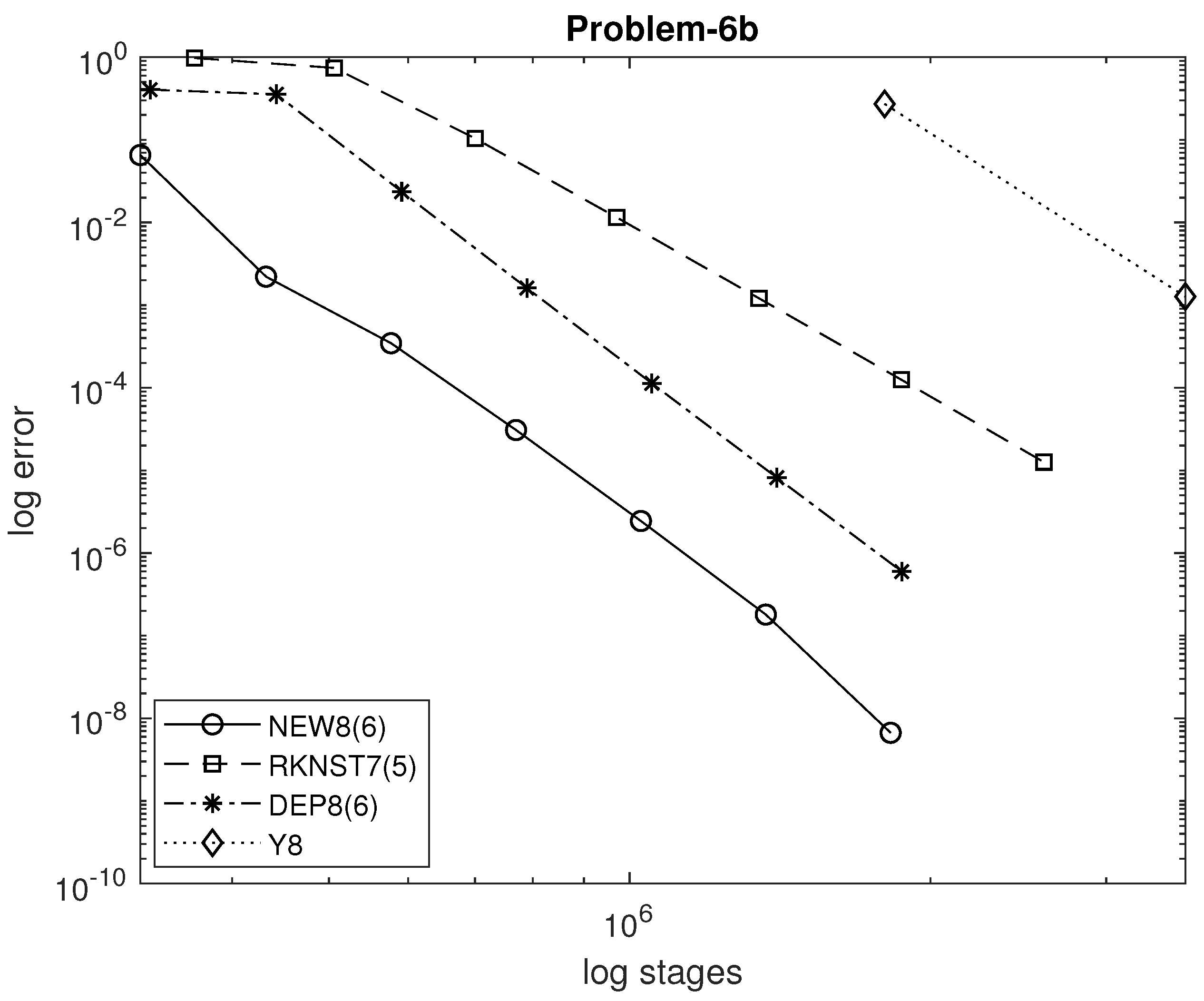
We run the methods NEW8(6), DEP8(6), RKNST7(5) and Y8 on problems 1b and 6b. The intervals of integration were lengthened to 10,000$\pi$ and 10,000$\pi /1.015$, respectively, in favor of symplectic methods. We recorded the stages taken versus the end-point error achieved and plot it in Figure 2 and Figure 3.

Figure 2. Efficiency curves for problem 1b in the interval [0, 10,000$\pi$].

Figure 3. Efficiency curves for problem 6b in the interval [0, 10,000$\pi$/1.015].

RKNTS7(5) pair was less efficient at higher tolerances than eighth order pairs since it attains lesser algebraic accuracy and it was not designed to perform best on Keplerian type orbits. DEP8(6) remains less efficient than NEW8(6) on these intervals and problems. Symplectic methods are not competitive at all. It seems to share interesting properties for geometers but not for numerical analysts. Their poor performance has already been remarked elsewhere [16].

7. Conclusions

In this study, we considered the Runge-Kutta-Nyström pairs of orders 8(6) for addressing the special second order Initial Value Problem. We focused on problems of the Keplerian type. Thus, we proposed a pair with coefficients specially trained in order to address such kinds of orbits. Extensive results justified our effort.