Dynamics of a Predator–Prey Model with the Additive Predation in Prey

Abstract

In this paper, we consider a predator–prey model, in which the prey’s growth is affected by the additive predation of its potential predators. Due to the additive predation term in prey, the model may exhibit the cases of the strong Allee effect, weak Allee effect and no Allee effect. In each case, the dynamics of global features of the model are investigated. Compared to the well-known Lotka–Volterra type model, the model proposed in this paper exhibits much richer and more complex dynamic behaviors, such as the Allee effect, the sensitivity to the initial conditions caused by the strong Allee effect, the oscillatory behavior and the Hopf and heteroclinic bifurcations. Furthermore, the stability and Hopf bifurcation of the model with the density dependent feedback time delay in prey are investigated. By the normal form method and center manifold theory, the explicit formulas are presented to determine the direction of Hopf bifurcation and the stability and period of Hopf-bifurcating periodic solutions. Theoretical analysis and numerical simulation indicate that the delay may destabilize the model, and cause the Hopf bifurcation not only at the interior equilibrium but also at a boundary equilibrium.

1. Introduction

Kang and Udiani [1] studied the evolutionary results of the following single population model involved with an additive predation

$$\frac{\mathrm{d}u}{\mathrm{d}t}=ru\left(1-\frac{u}{K}\right)-\frac{au}{1+mu},$$

(1)

where $r,K,a$ and m are positive parameters, r is the intrinsic growth rate, K is the carrying capacity of species in the absence of additive predation. When $a=0$, model (1) implies that the species u follows the logistic growth and the influence of its predator is not involved. In nature, there are few populations that do not have natural predators. Therefore, Equation (1) is an adjustment of logistic model, which models the dynamics of a single population affected by its predators. The influence of predators is described by the Holling type II functional response $au\left(t\right)/(1+mu(t\left)\right)$, which represents the positive correlation between the growth of the species u and its predators. In the case of predation satiation, a denotes the attack rate and $\frac{m}{a}$ is the handling time of predators [1,2,3].

Due to the additive predation term $au\left(t\right)/(1+mu(t\left)\right)$, model (1) can exhibit the Allee effect (called a component Allee effect or an additive Allee effect [1]). The Allee effect, first observed in the 1930s by Warder Clyde Allee [4,5], is a wide range of biological phenomenon of population growth. It presents the positive relationship between the mean individual fitness (often measured as per capita growth rate) and the size or density of the population [6,7,8,9,10,11,12]. Any mechanism leading to a positive relationship between a component of individual fitness and the number or density of conspecifics can be regarded as a mechanism of the Allee effect [11], such as mating difficulty, deficient feeding to low densities, environment conditioning and inbreeding depression, reduced defense against predators and many others [2,6,8,11,12]. The Allee effect can be divided into two main types: Strong Allee effect and weak Allee effect. See, for example [2,7,13,14,15,16]. At low density, if the per capita growth rate of a species is negative, then it is said that the population is affected by a strong Allee effect, otherwise it has a weak Allee effect. A strong Allee effect induces a threshold population, called Allee threshold, below which population growth decreases and goes to extinction and above which the population is persistent. A population with a weak Allee effect does not have such a critical threshold. The population models with different Allee effects have been widely studied. See, for example [2,12,17,18,19,20,21,22,23]. The models with a component Allee effect, of a type similar to (1), was first mentioned by Kostitizin [24] and applied in [2,11,25,26,27,28,29,30,31,32].

If the species u has multiple predators and we are only interested in the interaction between the species u and one of its predators, denoted by v, then the relationship between species u and v can be modeled by the following predator–prey system

$$\begin{array}{cc}\hfill & \frac{\mathrm{d}u\left(t\right)}{\mathrm{d}t}=ru\left(t\right)\left(1-\frac{u\left(t\right)}{K}\right)-\frac{au\left(t\right)}{1+mu\left(t\right)}-\alpha u\left(t\right)v\left(t\right),\hfill \\ \hfill & \frac{\mathrm{d}v\left(t\right)}{\mathrm{d}t}=\beta u\left(t\right)v\left(t\right)-dv\left(t\right),\hfill \end{array}$$

(2)

where $\alpha ,\beta ,d$ are positive constants that stand for the consumption rate, conversion rate and death rate of the predator v. In model (2), v is one of the many predators of the prey u that we are concerned about, and Holling type I functional response of the predator v is assumed, the influences of other predators on the growth of the prey u is described by $\frac{au\left(t\right)}{1+mu\left(t\right)}$.

In this paper, we will determine how the additive predation affects the dynamics of model (2) and mainly focus on the extinction and coexistence of the predator and prey species. Due to the additive predation, model (1), and hence (2), may exhibit the cases of the strong Allee effect, weak Allee effect and no Allee effect. For each case, the dynamics of the global features of (2) will be investigated. The ratio $\frac{a}{r}$ of the attack rate a of other potential predators to the intrinsic growth rate r of prey species u, and the ratio $\frac{d}{\beta }$ of the death rate d to the conversion rate $\beta$ of predator species play a key role in the dynamics of model (2). Our main results reveal the following dynamic features and the biological implications:

(i)

If the ratio $\frac{d}{\beta }$ exceeds the largest size that the prey u may eventually achieve, then the predator species goes extinct.

(ii)

When model (2) has the weak Allee effect or no Allee effect, if the ratio $\frac{d}{\beta }$ is below the largest size that the prey u may eventually achieve, both the predator and prey species may coexist. In the weak Allee effect case, the coexistence exhibits an oscillatory mode (when there exists a stable limit cycle) or steady state mode (when the interior equilibrium is globally asymptotically stable), while in the no Allee effect case, it is only the steady state mode. In the strong Allee effect, the extinction and coexistence depend on the initial population sizes of the prey and predator.

(iii)

For the strong Allee effect case, model (2) exhibits a more complex bifurcation phenomenon than the other cases, such as the Hopf and heteroclinic bifurcations. Due to the strong Allee effect caused by the additive predation term $\frac{au\left(t\right)}{1+mu\left(t\right)}$, the initial population sizes play an extremely important role in the dynamics of (2). For a set of parameter values, the extinction, coexistence, and population oscillations may be the result of different initial conditions.

(iv)

The main dynamics of model (2) can be described conclusively in a bifurcation diagram with respect to $(\frac{a}{r},\frac{d}{\beta })$.

(v)

Compared to the well-known Lotka–Volterra type model (when $a=0$), the additive predation term $\frac{au\left(t\right)}{1+mu\left(t\right)}$ leads model (2) to have much richer and more complex dynamical behaviors, such as the Allee effect, oscillatory behavior, a more complex bifurcation phenomenon and sensitivity to the initial conditions. The Lotka–Volterra type model only has the similar dynamic structure of model (2) in the case of no Allee effect.

The growth of an organism depends not only on its current state, but also on its past population density at a certain time; that is, a real system should be modeled by differential equations with time delays [33,34,35]. Time delay is one of the main factors in the ecological systems and has important influences on the stability of population dynamics [33,34,35,36,37,38]. When the effects of population density of species u on its birth rate at later times are considered, (2) becomes the following delayed predator–prey model

$$\begin{array}{cc}\hfill & \frac{\mathrm{d}u\left(t\right)}{\mathrm{d}t}=ru\left(t\right)\left(1-\frac{u(t-\tau )}{K}\right)-\frac{au\left(t\right)}{1+mu\left(t\right)}-\alpha u\left(t\right)v\left(t\right),\hfill \\ \hfill & \frac{\mathrm{d}v\left(t\right)}{\mathrm{d}t}=\beta u\left(t\right)v\left(t\right)-dv\left(t\right),\hfill \end{array}$$

(3)

where $\tau >0$ is the density dependent feedback time delay of the prey to the growth of the species itself. For model (3), we mainly investigate the stability and Hopf bifurcation induced by the delay $\tau$. The normal form method and the center manifold theory are applied to analyze the direction of Hopf bifurcation, and the stability and period of the Hopf-bifurcating periodic solutions.

The initial conditions of (3) are taken as follows:

$$\begin{array}{cc}\hfill & u\left(s\right)={\varphi }_1\left(s\right)\ge 0,v\left(s\right)={\varphi }_2\left(s\right)\ge 0,s\in [-\tau ,0],\hfill \\ \hfill & {\varphi }_1\left(0\right)>0,{\varphi }_2\left(0\right)>0,\hfill \end{array}$$

(4)

where $({\varphi }_1\left(s\right),{\varphi }_2\left(s\right))\in C([-\tau ,0],{\mathbb{R}}_{+}^2)$, $C([-\tau ,0],{\mathbb{R}}_{+}^2)$ is the Banach space of continuous functions mapping the interval $[-\tau ,0]$ into ${\mathbb{R}}_{+}^2$, ${\mathbb{R}}_{+}^2=\{(x_1,x_2)\in {\mathbb{R}}^2:x_i\ge 0,i=1,2\}$.

The rest of the paper is organized as follows. In Section 2, we present a brief sketch of the dynamics of the single population model (1) and show the parameter regions of the strong Allee effect, weak Allee effect and no Allee effect. Then in Section 3, for each case we discuss the dynamics of model (2), and analyze the influence of the additive predation term $\frac{au\left(t\right)}{1+mu\left(t\right)}$. In Section 4, we consider the delay model (3) and present the occurrence of Hopf bifurcation induced by the delay $\tau$. Furthermore, we use the normal form method and the center manifold theory to analyze the direction of Hopf bifurcation, and the stability and period of the Hopf-bifurcating periodic solutions. Some numerical simulations are presented to illustrate the theoretical analysis on the dynamics of the delayed predator–prey system (3). In Section 5, we briefly provide a summary of our results and compare the dynamics of model (2) with the dynamics of the well-known Lotka–Volterra type model (when $a=0$).

2. Dynamics of the Single Population Model

In order to have a complete understanding of the influence of the additive predation term $\frac{au\left(t\right)}{1+mu\left(t\right)}$ on the dynamics of model (2), in this section we consider the dynamics of the single population model (1). Let

$$H\left(u\right)=r\left(1-\frac{u}{K}\right)-\frac{a}{1+mu}.$$

(5)

It is easy to see that $H\left(u\right)$ has its local maximum at

$$u_0=\frac{1}{m}\left(\sqrt{\frac{amK}{r}}-1\right)>0,$$

(6)

and $H^{\prime }\left(u\right)=-\frac{r}{K}+\frac{am}{{(1+mu)}^2}<0$ for $u>u_0$ while $H^{\prime }\left(u\right)>0$ for $u<u_0$. Since $H^{\prime }\left(0\right)=-\frac{r}{K}+am$, we know that if the ratio of the attack rate a to the intrinsic growth rate r is large such that $\frac{a}{r}>\frac{1}{mK}$ holds, then model (1) may admit an Allee effect (see [1]).

Clearly, $u=0$ is a trivial equilibrium of (1). The positive equilibria are the positive roots of $H\left(u\right)=\frac{1}{1+mu}\tilde{H}\left(u\right)=0$, where

$$\tilde{H}\left(u\right):=-\frac{rm}{K}{u}^2+\frac{r}{K}(mK-1)u+r-a=0.$$

(7)

Let $\mathsf{\Delta }=\frac{r^2}{K^2}{(mK-1)}^2+4(r-a)\frac{rm}{K}$. If $\mathsf{\Delta }\ge 0$, i.e., $\frac{a}{r}\le \frac{{(mK+1)}^2}{4mK}$, Equation (7) has two real roots $u_1^{*}$ and $u_2^{*}$ ($u_1^{*}\le u_2^{*}$):

$$u_i^{*}=\frac{r(mK-1)\pm K\sqrt{\mathsf{\Delta }}}{2rm}=\frac{(mK-1)\pm \sqrt{{(mK-1)}^2+4mK(1-\frac{a}{r})}}{2m},i=1,2.$$

(8)

By (7) and (8), it is easy to get the existence and stability of positive equilibria of model (1) (see [1]). However, to better understand the influences of the additive predation term $\frac{au\left(t\right)}{1+mu\left(t\right)}$ on the dynamics of (1), we prefer the following analysis.

First, we show the following two cases in which the species tend to extinction.

(i)

If $\frac{a}{r}\ge 1$ and $\frac{1}{mK}\ge 1$, then for all $u>0$, $H\left(u\right)<0$, (1) has no positive equilibrium and $u=0$ is globally asymptotically stable, which implies that the species u will be extinct. For model (2), both species become extinct since the survival of the predator v only depends on the prey u.

(ii)

If $\mathsf{\Delta }<0$, i.e., $\frac{a}{r}>\frac{{(mK+1)}^2}{4mK}$, then the species u and hence v will be extinct since $H\left(u\right)<0$ for all $u>0$.

So, in what follows, the above two cases will not be discussed.

Now we consider the other cases as follows.

(a)

Assume $\frac{a}{r}>\frac{1}{mK}$.

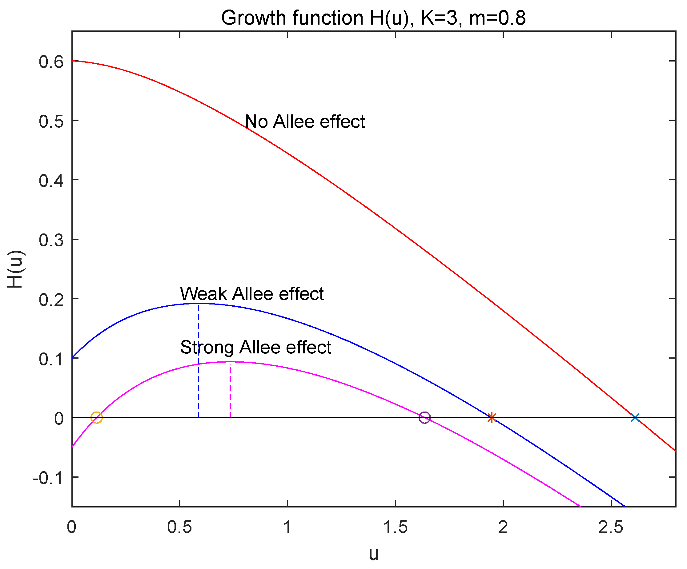
• If $1<\frac{a}{r}<\frac{{(mK+1)}^2}{4mK}$, which implies that $mK>1$, then $H\left(0\right)=r-a<0$, $H\left(u\right)$ has two positive roots $u=u_1^{*}$ and $u=u_2^{*}$, which are given by (8) and satisfy that $H^{\prime }\left(u_1^{*}\right)>0$ and $H^{\prime }\left(u_2^{*}\right)<0$ since $u_1^{*}<u_0<u_2^{*}$ (see Figure 1). Thus, $u=0$ is locally asymptotically stable, $u=u_1^{*}$ is unstable and $u=u_2^{*}$ is locally asymptotically stable. So, in this case, the strong Allee effect appears in population growth of (1) and $u=u_1^{*}$ is the Allee threshold. The species u will be extinct when the initial population size is below $u_1^{*}$, i.e., $u\left(0\right)<u_1^{*}$, and persistent when $u\left(0\right)>u_1^{*}$.
  

  Figure 1. The graph of $H\left(u\right)$.
• If $\frac{a}{r}<1$, then $H\left(0\right)>0$, $H\left(u\right)$ has one positive root $u=u_2^{*}$, satisfies that $H^{\prime }\left(u_2^{*}\right)<0$ and $0<u_0<u_2^{*}<K$ (see Figure 1). Thus, $u=0$ is unstable and $u=u_2^{*}$ is globally asymptotically stable. So, in this case, model (1) admits a weak Allee effect and the population is persistent.

(b)

Assume $\frac{a}{r}\le \frac{1}{mK}$, which implies that model (1) has no Allee effect, then $H^{\prime }\left(u\right)<0$ for all $u>0$. If $\frac{a}{r}<1$, $H\left(0\right)=r-a>0$ and $H\left(u\right)$ has one positive root $u=u_2^{*}$ (see Figure 1). It is clear that $0<u_2^{*}<K$. In this case, $u=0$ is unstable and $u=u_2^{*}$ is globally asymptotically stable.

Based on the above arguments, we define the parameter space $D=\{\nu =(a,r,m,K)\in {\mathbb{R}}_{+}^4:armK>0\}$ and (see Figure 2):

Figure 2. The parameter space D.

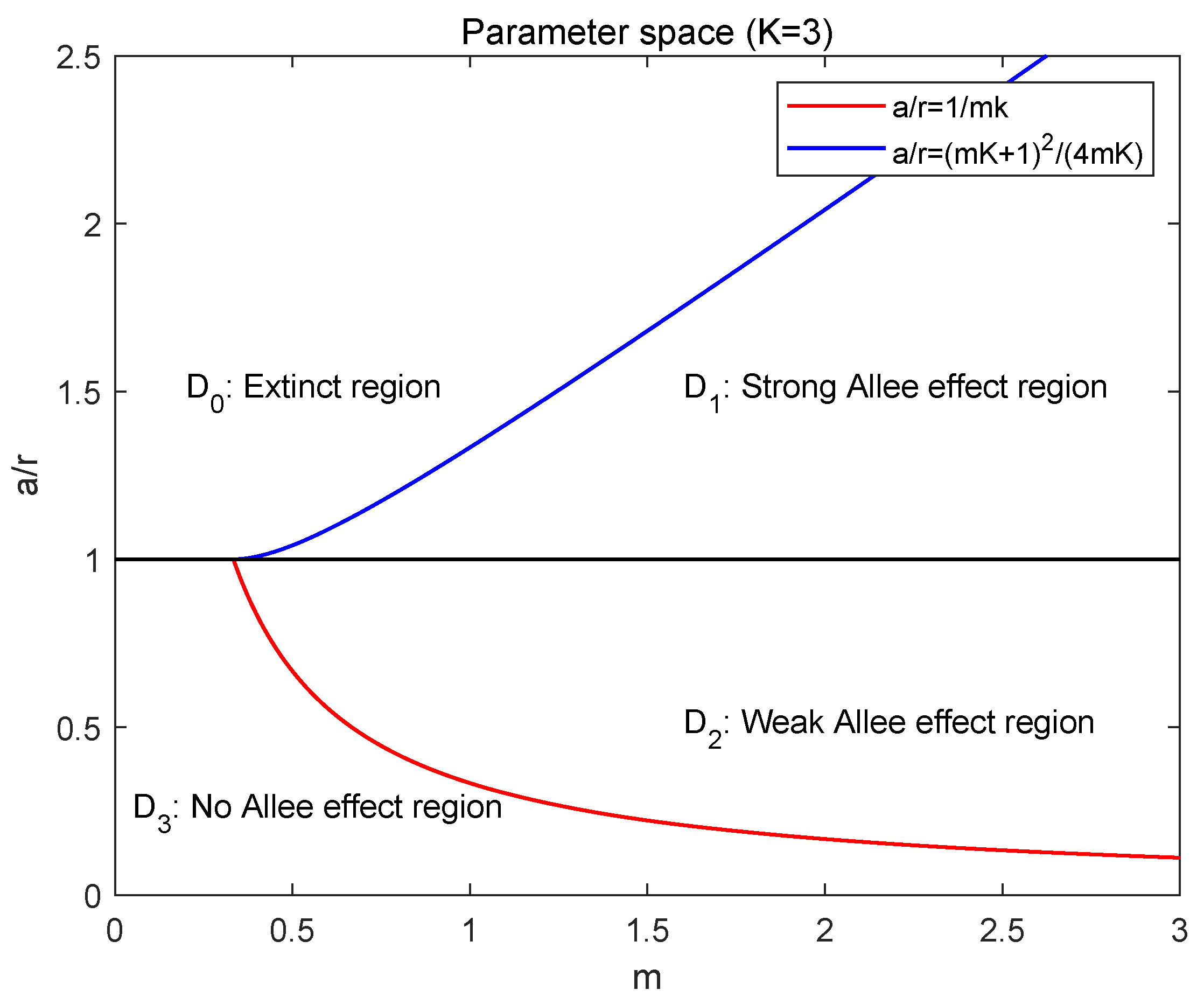
• Extinct region: $D_0=\{\nu \in D:\frac{a}{r}\ge 1,\frac{1}{mK}\ge 1\}\cup \{\frac{a}{r}>\frac{{(mK+1)}^2}{4mK}\}$,
• Strong Allee effect region: $D_1=\{\nu \in D:\frac{1}{mK}<1<\frac{a}{r}<\frac{{(mK+1)}^2}{4mK}\}$,
• Weak Allee effect region: $D_2=\{\nu \in D:\frac{1}{mK}<\frac{a}{r}<1\}$,
• No Allee effect region: $D_3=\{\nu \in D:\frac{a}{r}<1,\frac{a}{r}\le \frac{1}{mK}\}$.

From the above analysis, the ratio $\frac{a}{r}$ of the attack rate a of the additive predation to the intrinsic growth rate r of the species plays a key role in the dynamics of model (1). The large ratio $\frac{a}{r}$ goes against the population survival.

Define

$$b_1\left(u\right):=r\left(1-\frac{u}{K}\right)-\frac{a}{{(1+mu)}^2},b_2\left(u\right):=\frac{ru}{K}.$$

(9)

It is easy to see that

$$b_1\left(u\right)-b_2\left(u\right)={\left(uH\left(u\right)\right)}^{\prime }=H\left(u\right)+u{H}^{\prime }\left(u\right).$$

If u is a positive root of $H\left(u\right)$, then $b_1\left(u\right)=\frac{amu}{{(1+mu)}^2}$ and $b_1\left(u\right)-b_2\left(u\right)=u{H}^{\prime }\left(u\right)$. Thus, we have the following result, which will be used in the later arguments.

Lemma 1.

If $u_1^{*}$ and $u_2^{*}$ exist, then $b_1\left(u_1^{*}\right)-b_2\left(u_1^{*}\right)>0$ and $b_1\left(u_2^{*}\right)-b_2\left(u_2^{*}\right)<0$.

In the later arguments, we always assume that $\nu =(a,r,m,K)\in D_i,i=1,2,3$; that is, model (2) has a strong Allee effect, weak Allee effect or no Allee effect.

3. Dynamics of the Predator–Prey Model

Now we consider the dynamics of model (2). Define the state space of (2) as $X=\{(u,v)\in {\mathbb{R}}_{+}^2\}$ with its interior $\mathring{X}=\{(u,v)\in {\mathbb{R}}_{+}^2:uv>0\}$.

3.1. Positivity and Boundedness

Theorem 1.

1. Both X and $\mathring{X}$ are the positively invariant sets of model (2).

2. Model (2) is uniformly ultimately bounded in X, and $\underset{t\to \infty }{lim\; sup}u\left(t\right)\le u_2^{*}$.

Proof. 

1. For $u\ge 0$ and $v\ge 0$, we have $u^{\prime }{{|}_{u=0}=0,v^{\prime }|}_{v=0}=0$, which implies that both $u=0$ and $v=0$ are invariant manifolds. Due to the continuity of model (2), we can conclude that (2) is positively invariant in X and $\mathring{X}$.

2. From the arguments on the function $H\left(u\right)$ in Section 2, for the strong or weak Allee effect case, or no Allee effect case, $H\left(u\right)$ has a positive root $u_2^{*}$ such that $H\left(u\right)<0$ for $u>u_2^{*}$. Thus, by the positivity of (2), the first equation of (2) yields $u^{\prime }{\left(t\right)|}_{u=u_2^{*}}=-\alpha uv\le 0$ and $u^{\prime }{\left(t\right)|}_{u>u_2^{*}}=uH\left(u\right)-\alpha uv\le 0$. This implies $\underset{t\to +\infty }{lim}u\left(t\right)\le u_2^{*}$. Then, for any $ϵ>0$, there exists $T>0$ such that for $t>T$, $u\left(t\right)\le u_2^{*}+ϵ$. Let $W\left(t\right)=\frac{1}{\alpha }u+\frac{1}{\beta }v$, then $W^{\prime }\left(t\right)\le -dW\left(t\right)+\frac{d+r}{\alpha }(u_2^{*}+ϵ)$, $t>T$. It follows that $\underset{t\to \infty }{lim\; sup}W\left(t\right)\le \frac{d+r}{d\alpha }{u}_2^{*}$. Hence, model (2) is uniformly ultimately bounded in X. □

Remark 1.

Theorem 1 indicates that the population size of prey u ultimately cannot go beyond $u_2^{*}$. That is to say, $u_2^{*}$ is the largest size that the prey u may eventually achieve.

3.2. Equilibria

From the arguments on the single model (1) in Section 2, model (2) always has the trivial boundary equilibrium $E_0(0,0)$, and has at most two semi-trivial equilibria $E_1(u_1^{*},0)$ and $E_2(u_2^{*},0)$, where $u_1^{*}$ and $u_2^{*}$ are the positive roots of $H\left(u\right)=0$, defined as (8).

When $H(\frac{d}{\beta })>0$, model (2) has the unique positive equilibrium $E_{in}(u^{*},v^{*})$, where

$$u^{*}=\frac{d}{\beta },v^{*}=\frac{1}{\alpha }H\left(u^{*}\right)=\frac{r(K-u^{*})(1+m{u}^{*})-aK}{\alpha K(1+m{u}^{*})}.$$

(10)

3.3. Dynamics of the Strong Allee Effect Case

In this subsection, we consider the dynamics of model (2) in the strong Allee effect case. First we show the existence and local stability of equilibria, and that the Hopf bifurcation occurred at the positive equilibrium $E_{in}(u^{*},v^{*})$. Then we prove the non-existence of limit cycle when $u_1^{*}<\frac{d}{\beta }<u_0$, and discuss the extinction of (2). In addition, based on these arguments and numerical simulations, the dynamics of global features of (2) are presented.

The linearized matrix of (2) with respect to any of its equilibria $(u_{*},v_{*})$ can be expressed as

$$J=\begin{array}{c}\hfill \left(\begin{array}{cc}r(1-\frac{2u_{*}}{K})-\alpha v_{*}-\frac{a}{{(1+m{u}_{*})}^2}& -\alpha u_{*}\\ \beta v_{*}& \beta u_{*}-d\end{array}\right)=\left(\begin{array}{cc}{\left(uH\left(u\right)\right)}^{\prime }{|}_{u_{*}}-\alpha v_{*}& -\alpha u_{*}\\ \beta v_{*}& \beta u_{*}-d\end{array}\right),\end{array}$$

(11)

where

$$\begin{array}{c}\hfill {\left(uH\left(u\right)\right)}^{\prime }{|}_{u_{*}}-\alpha v_{*}=\left\{\begin{array}{cccc}& u_{*}{H}^{\prime }\left(u_{*}\right),\hfill & & \mathrm{at}{E}_1(u_1^{*},0),E_2(u_2^{*},0),E_{in}(u^{*},v^{*}),\hfill \\ & H\left(0\right)=r-a,\hfill & & \mathrm{at}{E}_0(0,0).\hfill \end{array}\right.\end{array}$$

(11) gives the characteristic equation

$${\lambda }^2-\mathrm{Tr}J\lambda +\mathrm{Det}J=0.$$

(12)

Lemma 2.

$E_{in}$, if it exists, is locally asymptotically stable when $H^{\prime }\left(u^{*}\right)<0$, and unstable when $H^{\prime }\left(u^{*}\right)>0$.

Proof. 

At $E_{in}(u^{*},v^{*})(u^{*}=\frac{d}{\beta })$, the characteristic Equation (12) becomes

$${\lambda }^2-u^{*}{H}^{\prime }\left(u^{*}\right)\lambda +\alpha d{v}^{*}=0.$$

(13)

So the result is clear. □

Theorem 2.

If model (2) exhibits the strong Allee effect, i.e., $\frac{1}{mK}<1<\frac{a}{r}<\frac{{(mK+1)}^2}{4mK}$, then the following statements hold.

1.

Model (2) has three boundary equilibria $E_0(0,0)$, $E_1(u_1^{*},0)$ and $E_2(u_2^{*},0)$. The positive equilibrium $E_{in}(u^{*},v^{*})$ exists if and only if $u_1^{*}<\frac{d}{\beta }<u_2^{*}$.

2.

$E_0(0,0)$ is a stable node.

3.

If $u_1^{*}<\frac{d}{\beta }$, $E_1(u_1^{*},0)$ is a saddle with its unstable manifold along the u axis and its stable manifold (denoted by ${\mathsf{\Gamma }}_{E_1}^s$) entering from the interior of ${\mathbb{R}}_{+}^2$; if $u_1^{*}>\frac{d}{\beta }$, $E_1(u_1^{*},0)$ is an unstable node.

4.

If $u_2^{*}>\frac{d}{\beta }$, $E_2(u_2^{*},0)$ is saddle with its stable manifold along the u axis and its unstable manifold (denoted by ${\mathsf{\Gamma }}_{E_2}^u$) entering the interior of ${\mathbb{R}}_{+}^2$; if $u_2^{*}<\frac{d}{\beta }$, $E_2(u_2^{*},0)$ is a stable node.

5.

The positive equilibrium $E_{in}(u^{*},v^{*})$ is locally asymptotically stable when $u_0<\frac{d}{\beta }<u_2^{*}$ and unstable when $u_1^{*}<\frac{d}{\beta }<u_0$. When $\frac{d}{\beta }=u_0$, model (2) undergoes the Hopf bifurcation at $E_{in}(u^{*},v^{*})$.

Proof. 

From the arguments of the function $H\left(u\right)$ in Section 2, in the strong Allee effect case, model (2) has three boundary equilibria $E_0(0,0)$, $E_1(u_1^{*},0)$ and $E_2(u_2^{*},0)$. Since $H\left(u\right)>0$ when $u_1^{*}<u<u_2^{*}$, by (10), we know that the positive equilibrium $E_{in}(u^{*},v^{*})$ exists if and only if $u_1^{*}<\frac{d}{\beta }<u_2^{*}$.

At $E_0(0,0)$, (12) has the eigenvalues ${\lambda }_1=H^{\prime }\left(0\right)=r-a$ and ${\lambda }_2=-d$. Thus, $E_0(0,0)$ is a stable node since $\frac{a}{r}>1$.

At the semi-trivial boundary equilibrium $E_i(u_i^{*},0),i=1,2$, the characteristic Equation (12) becomes

$$(\lambda -u_i^{*}{H}^{\prime }\left(u_i^{*}\right))(\lambda -(\beta u_i^{*}-d))=0,$$

(14)

which gives two eigenvalues ${\lambda }_1=u_i^{*}{H}^{\prime }\left(u_i^{*}\right)=b_1\left(u_i^{*}\right)-b_2\left(u_i^{*}\right)$ and ${\lambda }_2=\beta u_i^{*}-d$, where $b_1\left(u\right),b_2\left(u\right)$ are defined as (9). At $E_1(u_1^{*},0)$, by Lemma 1, ${\lambda }_1>0$ and hence the third part of the result holds. At $E_2(u_2^{*},0)$, ${\lambda }_1<0$, so the fourth part also holds.

In the strong Allee effect case, from the arguments on the function $H\left(u\right)$ in Section 2, $H^{\prime }\left(u\right)>0$ for $u_1^{*}<u<u_0$ and $H^{\prime }\left(u\right)<0$ for $u_0<u<u_2^{*}$. Then, by Lemma 2, the positive equilibrium $E_{in}(u^{*},v^{*})(u^{*}=\frac{d}{\beta })$ is locally asymptotically stable when $u_0<\frac{d}{\beta }<u_2^{*}$ and unstable when $u_1^{*}<\frac{d}{\beta }<u_0$.

When $\frac{d}{\beta }=u_0$, the characteristic Equation (13) has a pair of imaginary eigenvalues $\lambda =\pm i\omega ,\omega =\sqrt{\alpha d{v}^{*}}$. Then, the Hopf bifurcation occurs at $E_{in}(u^{*},v^{*})$. In fact, by taking $\frac{d}{\beta }$ as bifurcation parameter, we have $\frac{\partial \left(u^{*}{H}^{\prime }\left(u^{*}\right)\right)}{\partial (\frac{d}{\beta })}=\frac{\partial \left(u^{*}{H}^{\prime }\left(u^{*}\right)\right)}{\partial u^{*}}=u^{*}{H}^{″}\left(u^{*}\right)+H^{\prime }\left(u^{*}\right)$ since $u^{*}=\frac{d}{\beta }$. Notice that $H^{\prime }\left(u_0\right)=0$ and $H^{″}\left(u_0\right)<0$ since $H\left(u\right)$ is concave. Thus, $\frac{\partial \left(u^{*}{H}^{\prime }\left(u^{*}\right)\right)}{\partial (\frac{d}{\beta })}{{|}_{\frac{d}{\beta }=u_0}=(u^{*}{H}^{″}\left(u^{*}\right)+H^{\prime }\left(u^{*}\right))|}_{u^{*}=u_0}<0$, which implies from the Poincaré–Andronov–Hopf Bifurcation Theorem [39] that model (2) undergoes a Hopf bifurcation at $E_{in}(u^{*},v^{*})$ when $\frac{d}{\beta }=u_0=\frac{1}{m}\left(\sqrt{\frac{amK}{r}}-1\right)$. □

Remark 2.

From Theorem 2, we know that in the strong Allee effect case, if $u_0<\frac{d}{\beta }<u_2^{*}$, model (2) has two attractors $E_0\cup E_{in}$ (see Figure 3d–f); if $\frac{d}{\beta }>u_2^{*}$, model (2) has two attractors $E_0\cup E_2$ (see Figure 3g).

Figure 3. The dynamic behaviors of model (2) in the strong Allee effect case as $\frac{d}{\beta }$ varies ($\beta =1$). Here, parameters $K=3,m=2.5,\alpha =1,\frac{a}{r}=2(a=2,r=1)$. The heteroclinic bifurcation point $d_{\beta }^{*}=1.14915$. $u_1^{*}=0.6,u_0=1.14915,u_2^{*}=2$.

Theorem 3.

If model (2) exhibits the strong Allee effect, then (2) has no limit cycle when $u_1^{*}<\frac{d}{\beta }<u_0$ (see Figure 3b).

Proof. 

When $u_1^{*}<\frac{d}{\beta }<u_0$, according to Theorem 2, $E_0(0,0)$ is a stable node, both $E_1(u_1^{*},0)$ and $E_2(u_2^{*},0)$ are saddle, the positive equilibrium $E_{in}(u^{*},v^{*})(u^{*}=\frac{d}{\beta })$ exists and is unstable. Assume that model (2) has a periodic orbit $\left(u\right(t),v(t\left)\right)$ with period T. Then, by integrating the equations of (2) on $[0,T]$, we have

$$\begin{array}{c}\hfill \alpha {\int }_0^{T}v\left(t\right)dt={\int }_0^{T}H\left(u\left(t\right)\right)dt,{\int }_0^T(\beta u\left(t\right)-d)dt=0.\end{array}$$

(15)

Denote the right-hand sides of (2) as $P_1(u,v)$ and $P_2(u,v)$, respectively. By (15), we get the integral of divergence of (2):

$$\begin{array}{cc}\hfill {\int }_0^T\left(\frac{\partial P_1}{\partial u}+\frac{\partial P_2}{\partial v}\right)dt& ={\int }_0^{T}u\left(t\right)H^{\prime }\left(u\left(t\right)\right)dt.\end{array}$$

(16)

Let $M_0=(u_0,0)$ and $M_1=(u_0,\frac{1}{\alpha }H\left(u_0\right))$. We consider the positive half-trajectory ${\gamma }^{+}\left(M_1\right)$ passing the point $M_1$. By examining the direction of the vector field in model (2), ${\gamma }^{+}\left(M_1\right)$ must pass the v-nullcline $u=u^{*}=\frac{d}{\beta }$ above the u-nullcline $v=\frac{1}{\alpha }H\left(u\right)$ and enter the region $\{(u,v)\in {\mathbb{R}}_{+}^2\mid v>\frac{1}{\alpha }H\left(u\right),u<\frac{d}{\beta }\}$.

If ${\gamma }^{+}\left(M_1\right)$ does not enter the region $\{(u,v)\in {\mathbb{R}}_{+}^2\mid v<\frac{1}{\alpha }H\left(u\right)\}$, then ${\gamma }^{+}\left(M_1\right)$ must intersect the line $u=u_1^{*}$ at some point $M_2$. Thus, we can construct a region $\mathcal{R}$ with the vertices $M_0,M_1,M_2$ and $E_1$ as follows: Between $M_1$ and $M_2$, the boundary of $\mathcal{R}$ is the orbit ${\gamma }^{+}\left(M_1\right)$, and all other parts of the boundary of $\mathcal{R}$ are the line segments connecting $M_1\to M_0\to E_1\to M_2$. It is easy to see that $\mathcal{R}$ is negatively invariant. Since $E_{in}$ is the unique equilibrium point in the first quadrant, any periodic orbit, if it exists, must encircle it and lie wholly in the region $\mathcal{R}$. Assume $\left(u\right(t),v(t\left)\right)$ is a T-periodic orbit in $\mathcal{R}$. Then $u\left(t\right)<u_0$ and hence $H^{\prime }\left(u\left(t\right)\right)>0$. Thus, ${\int }_0^T\left(\frac{\partial P_1}{\partial u}+\frac{\partial P_2}{\partial v}\right)dt>0$ from (16). This implies that the periodic orbit is unstable. However, it is impossible since $E_{in}$ is unstable.

Assume that ${\gamma }^{+}\left(M_1\right)$ enters the region $\{(u,v)\in {\mathbb{R}}_{+}^2\mid v<\frac{1}{\alpha }H\left(u\right)\}$. After that, if ${\gamma }^{+}\left(M_1\right)$ always stays on the left of the line $u=u_0$, then its $\omega$-limit set must be a periodic orbit. From (16) the periodic orbit is unstable. However, this is also impossible since $E_{in}$ is unstable. If ${\gamma }^{+}\left(M_1\right)$ intersects the line $u=u_0$ at some point $M_2$, then we can construct the region $\mathcal{R}$ as follows: Its boundaries are composed of the segment of orbit ${\gamma }^{+}\left(M_1\right)$ from $M_1$ to $M_2$ and the straight line segment $u=u_0$ between $M_1$ and $M_2$. Clearly, $\mathcal{R}$ is negatively invariant. Similar to the above arguments, model (2) has no periodic orbit. □

Remark 3.

From Theorems 2 and 3, we can conclude that when $\frac{d}{\beta }=u_0$, the forward and subcritical Hopf bifurcation occurs at the positive equilibrium $E_{in}(u_0,\frac{1}{\alpha }H\left(u_0\right))$ (see Figure 3). That is, as $\frac{d}{\beta }$ increases from $u_0$, model (2) has an unstable limit cycle bifurcating from the positive equilibrium $E_{in}(u_0,\frac{1}{\alpha }H\left(u_0\right))$. When $u_0<\frac{d}{\beta }<u_2^{*}$, both $E_1(u_1^{*},0)$ and $E_2(u_2^{*},0)$ are saddle, and model (2) may have a heteroclinic orbit connecting $E_2$ to $E_1$ (see Figure 3e).

Now we show the extinction of model (2).

Theorem 4.

If model (2) exhibits the strong Allee effect, then (2) has the following dynamics.

1.

If $\frac{d}{\beta }>u_2^{*}$, then the population v goes extinct (see Figure 3g).

2.

If $\frac{d}{\beta }<u_1^{*}$, then both species u and v go extinct (see Figure 3a).

3.

If $u\left(0\right)\le u_1^{*}$, then both species u and v go extinct.

Proof. 

Let $\frac{d}{\beta }>u_2^{*}$. By $\underset{t\to +\infty }{lim\; sup}u\left(t\right)\le u_2^{*}$ from Theorem 1, we have that for sufficiently small $ϵ>0$ satisfying $\frac{d}{\beta }>u_2^{*}+ϵ$, there exists $T>0$ such that for all $t>T$, $u\left(t\right)\le u_2^{*}+ϵ$. Then by the second equation of (2), we have that $v^{\prime }=v(\beta u-d)\le v(\beta (u_2^{*}+ϵ)-d)\le 0,\forall t>T$. It follows that $\underset{t\to \infty }{lim}v\left(t\right)=0$.

If $\frac{d}{\beta }<u_1^{*}$, then according to Theorem 2, model (2) only has three boundary equilibria $E_0(0,0)$, $E_1(u_1^{*},0)$ and $E_2(u_2^{*},0)$, where $E_0$ is a stable node, $E_1$ is an unstable node and $E_2$ is a saddle. Theorem 1 implies that (2) has a compact global attractor. Thus, from an application of the Poincaré–Bendixson theorem [40] we conclude that $\underset{t\to \infty }{lim}(u\left(t\right),v\left(t\right))=0$ for any solution $\left(u\right(t),v(t\left)\right)$ of (2) initiated from the interior of ${\mathbb{R}}_{+}^2$; that is, $E_0$ is globally asymptotically stable.

Assume $u\left(0\right)\le u_1^{*}$. From the first equation of (2), we have $u^{\prime }{|}_{u<u_1^{*}}\le 0$ and $u^{\prime }{|}_{u=u_1^{*}}\le 0$, which implies $\underset{t\to \infty }{lim}u\left(t\right)=0$. Thus, the second equation of (2) yields $\underset{t\to \infty }{lim}v\left(t\right)=0$. □

Remark 4.

Theorem 4 indicates the following biological implications.

i.

The first part is about the extinction of predator species due to the large ratio $\frac{d}{\beta }$ of the death rate d to the conversion rate β of predator species.

ii.

The second part is about the extinction due to the strong Allee effect of the prey population driven by the additive predation $\frac{au\left(t\right)}{1+mu\left(t\right)}$. $\frac{d}{\beta }<u_1^{*}$ implies that the invasion or reproduction of the predator v is excessive while the reproduction of the prey u is not fast enough to sustain its own population. Thus, the excessive invasion or reproduction of the predator v drives the population of the prey u to below its Allee threshold and eventually to zero, which consequently drives the predator population to extinction.

iii.

The third statement indicates that when the population density of the prey is below its Allee threshold $u_1^{*}$, all species will be extinct.

Now, let $K,m,\alpha$ and $\frac{a}{r}$ be fixed such that model (2) exhibits the strong Allee effect. By the previous discussion and numerical simulations, as $\frac{d}{\beta }$ varies, we show the dynamics of global features of (2) (see Figure 3).

(i)

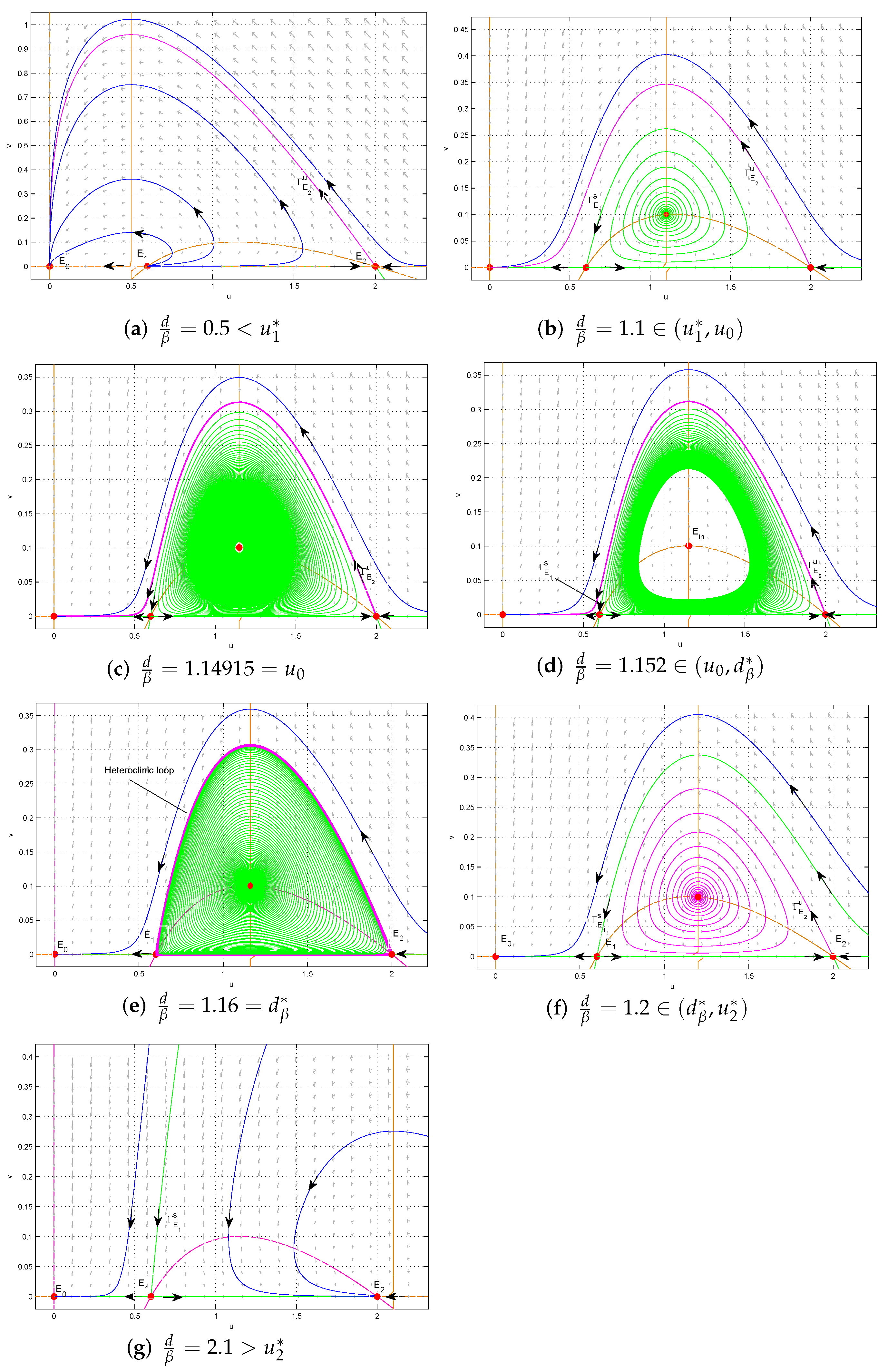
$\frac{d}{\beta }<u_1^{*}$. $E_0$ is a stable node, $E_1$ is an unstable node, $E_2$ is a saddle. There is no interior equilibrium. All trajectories in the interior of ${\mathbb{R}}_{+}^2$ converge to $E_0$; two species will be extinct (see Figure 3a).

(ii)

$u_1^{*}<\frac{d}{\beta }<u_0$. $E_1$ becomes a saddle and an unstable interior equilibrium $E_{in}$ appears. Around $E_{in}$, there is no limit cycle. Except for the stable manifold ${\mathsf{\Gamma }}_{E_1}^s$ of $E_1$, all trajectories converge to $E_0$ (see Figure 3b).

(iii)

$\frac{d}{\beta }=u_0$. A forward subcritical Hopf bifurcation occurs (see Figure 3c).

(iv)

$u_0<\frac{d}{\beta }<u_2^{*}$. Both $E_1$ and $E_2$ are saddle and the interior equilibrium $E_{in}$ become locally asymptotically stable. There exists a threshold value $d_{\beta }^{*}:u_0<d_{\beta }^{*}<u_2^{*}$ such that

(a)

when $u_0<\frac{d}{\beta }<d_{\beta }^{*}$, there exists an unstable limit cycle surrounding $E_{in}$. Outside the limit cycle, two species cannot coexist, while inside the limit cycle trajectories converge towards the stable interior equilibrium $E_{in}$ (see Figure 3d);

(b)

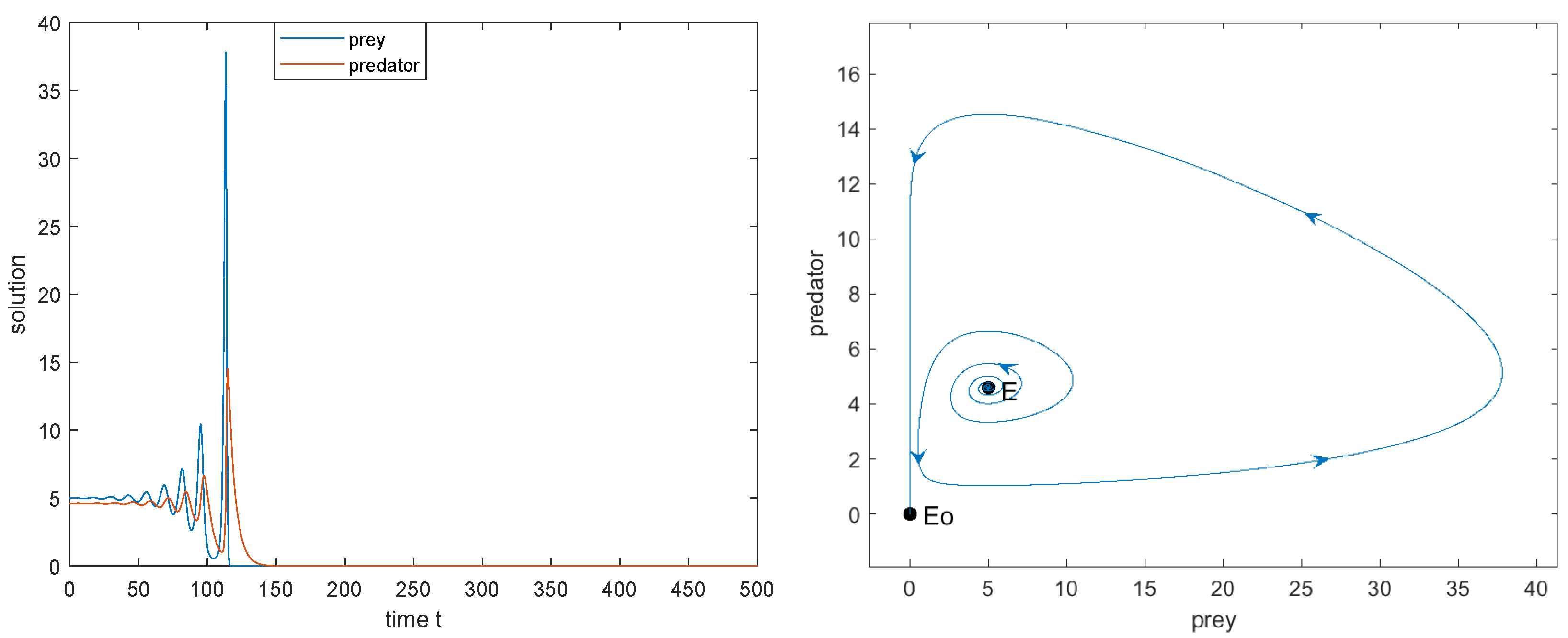
when $\frac{d}{\beta }=d_{\beta }^{*}$, the limit cycle disappears and a heteroclinic loop connecting $E_2$ to $E_1$ appears. Outside the heteroclinic loop, trajectories converge to $E_0$, and two species will be extinct, while inside the heteroclinic loop trajectories converge towards the heteroclinic loop, and two species coexist (see Figure 3e);

(c)

when $d_{\beta }^{*}<\frac{d}{\beta }<u_2^{*}$, the heteroclinic orbit is broken. Above the stable manifold ${\mathsf{\Gamma }}_{E_1}^s$ of $E_1$, trajectories converge to $E_0$, and two species will be extinct, while below ${\mathsf{\Gamma }}_{E_1}^s$, trajectories converge towards the stable interior equilibrium $E_{in}$, and two species coexist (see Figure 3f).

(v)

$\frac{d}{\beta }>u_2^{*}$. There is a transcritical bifurcation at $\frac{d}{\beta }=u_2^{*}$. When increasing the value of $\frac{d}{\beta }$ from $u_2^{*}$, $E_2$ becomes a stable node and the interior equilibrium $E_{in}$ disappears. This leads to the predator free dynamics with $E_0\cup E_2$ as attractors (see Figure 3g).

3.4. Dynamics of the Weak Allee Effect Case

In this subsection, we consider the dynamics of model (2) in the weak Allee effect case, including the existence of equilibria, the local dynamics and the global feature of (2).

First, we show the existence and local stability of equilibria.

Theorem 5.

If model (2) exhibits the weak Allee effect, i.e., $1>\frac{a}{r}>\frac{1}{mK}$, then the following statements holds.

1.

Model (2) has two boundary equilibria $E_0(0,0)$ and $E_2(u_2^{*},0)$. The positive equilibrium $E_{in}(u^{*},v^{*})$ exists if and only if $0<\frac{d}{\beta }<u_2^{*}$.

2.

$E_0(0,0)$ is always an unstable saddle.

3.

$E_2(u_2^{*},0)$ is a stable node when $u_2^{*}<\frac{d}{\beta }$ and an unstable saddle when $u_2^{*}>\frac{d}{\beta }$.

4.

The positive equilibrium $E_{in}(u^{*},v^{*})$ is locally asymptotically stable when $u_0<\frac{d}{\beta }<u_2^{*}$ and unstable when $0<\frac{d}{\beta }<u_0$. When $\frac{d}{\beta }=u_0$, system (2) undergoes the Hopf bifurcation at $E_{in}(u^{*},v^{*})$.

Proof. 

In the weak Allee effect case, by the property of $H\left(u\right)$ shown in Section 2, model (2) has two boundary equilibria $E_0(0,0)$ and $E_2(u_2^{*},0)$. The positive equilibrium $E_{in}(u^{*},v^{*})$ exists if and only if $u_1^{*}<\frac{d}{\beta }<u_2^{*}$.

At $E_0(0,0)$, (12) has the eigenvalues ${\lambda }_1=H^{\prime }\left(0\right)=r-a>0$ and ${\lambda }_2=-d$. Thus, $E_0(0,0)$ is a saddle.

At $E_2(u_2^{*},0)$, the characteristic Equation (14) has two eigenvalues ${\lambda }_1=u_2^{*}{H}^{\prime }\left(u_2^{*}\right)=b_1\left(u_2^{*}\right)-b_2\left(u_2^{*}\right)$ and ${\lambda }_2=\beta u_2^{*}-d$. By Lemma 1, ${\lambda }_1<0$. Thus, $E_2$ is a stable node when $u_2^{*}<\frac{d}{\beta }$ and a saddle when $u_2^{*}>\frac{d}{\beta }$.

In the weak Allee effect case, from the property of $H\left(u\right)$ shown in Section 2, $H^{\prime }\left(u\right)>0$ for $0<u<u_0$ and $H^{\prime }\left(u\right)<0$ for $u_0<u<u_2^{*}$. Then, by Lemma 2, the positive equilibrium $E_{in}(u^{*},v^{*})(u^{*}=\frac{d}{\beta })$ is locally asymptotically stable when $u_0<\frac{d}{\beta }<u_2^{*}$ and unstable when $0<\frac{d}{\beta }<u_0$.

When $\frac{d}{\beta }=u_0$, similar to the arguments of the strong Allee effect case, the Hopf bifurcation occurs at $E_{in}(u^{*},v^{*})$. □

Now we state the global dynamic behavior of model (2) (see Figure 4).

Figure 4. The dynamics of model (2) in the case of weak Allee effect as $\frac{d}{\beta }$ varies ($\beta =1$). Here, $K=3$, $m=1.5,\alpha =1,\frac{a}{r}=2(a=0.8,r=1)$. $u_0=0.5982,u_2^{*}=2.4937$.

Theorem 6.

If model (2) exhibits the weak Allee effect, then the following dynamics hold.

1.

If $\frac{d}{\beta }>u_2^{*}$, then $E_2(u_2^{*},0)$ is globally asymptotically stable (see Figure 4d).

2.

If $u_0<\frac{d}{\beta }<u_2^{*}$, then $E_{in}(u^{*},v^{*})$ is globally asymptotically stable (see Figure 4c).

3.

If $0<\frac{d}{\beta }<u_0$, then model (2) has a stable limit cycle surrounding $E_{in}(u^{*},v^{*})$ (see Figure 4a).

Proof. 

1. In the weak Allee effect case and $\frac{d}{\beta }>u_2^{*}$, by Theorem 5, model (2) has two boundary equilibria $E_0(0,0)$ and $E_2(u_2^{*},0)$, in which $E_0(0,0)$ is a saddle and $E_2(u_2^{*},0)$ is a stable node, and has no positive equilibrium. Thus, from an application of Poincaré–Bendixson theorem [40] we conclude that $E_2(u_2^{*},0)$ is globally asymptotically stable.

2. When $u_0<\frac{d}{\beta }<u_2^{*}$, both $E_0(0,0)$ and $E_2(u_2^{*},0)$ are saddle, and $E_{in}(u^{*},v^{*})$ exists and is locally asymptotically stable by Theorem 5. The stable and unstable manifolds of $E_0$ are along the v-axis and u-axis, respectively. The stable manifold of $E_2$ is along the u-axis and its unstable manifold enters the interior of ${\mathbb{R}}_{+}^2$. If (2) has no limit cycle, then from Poincaré–Bendixson theorem [40] we can conclude that $E_{in}$ is globally asymptotically stable. On the contrary, we assume that model (2) has a periodic orbit $\left(u\right(t),v(t\left)\right)$ with period T. Then, (16) holds.

Let $M_0=(u_0,0)$ and $M_1=(u_0,\frac{1}{\alpha }H\left(u_0\right))$. We consider the negative half-trajectory ${\gamma }^{-}\left(M_1\right)$ passing the point $M_1$. By examining the direction of vector field in model (2), ${\gamma }^{-}\left(M_1\right)$ must pass the v-nullcline $u=u^{*}=\frac{d}{\beta }$ above the u-nullcline $v=\frac{1}{\alpha }H\left(u\right)$ and enter the region $\{(u,v)\in {\mathbb{R}}_{+}^2\mid v>\frac{1}{\alpha }H\left(u\right),u>\frac{d}{\beta }\}$.

If ${\gamma }^{-}\left(M_1\right)$ does not enter the region $\{(u,v)\in {\mathbb{R}}_{+}^2\mid v<\frac{1}{\alpha }H\left(u\right)\}$, then ${\gamma }^{-}\left(M_1\right)$ must intersect the line $u=u_2^{*}$ at some point $M_2$. Thus, we can construct a region ${\mathcal{R}}_1$ with the vertices $M_0,M_1,M_2$ and $E_2$ as follows: Between $M_1$ and $M_2$, the boundary of ${\mathcal{R}}_1$ is the orbit ${\gamma }^{-}\left(M_1\right)$, and all other parts of the boundary of ${\mathcal{R}}_1$ are the line segments connecting $M_1\to M_0\to E_1\to M_2$. It is easy to see that ${\mathcal{R}}_1$ is positively invariant. Since $E_{in}$ is the unique equilibrium point in the first quadrant, any periodic orbit, if it exists, must encircle it and lie wholly in the region ${\mathcal{R}}_1$. Assume $\left(u\right(t),v(t\left)\right)$ is a T-periodic orbit in ${\mathcal{R}}_1$. Then $u\left(t\right)>u_0$ and hence $H^{\prime }\left(u\left(t\right)\right)<0$. Thus, ${\int }_0^T\left(\frac{\partial P_1}{\partial u}+\frac{\partial P_2}{\partial v}\right)dt<0$ from (16). This implies that the periodic orbit is stable. However, it is impossible since $E_{in}$ is locally asymptotically stable.

Assume that ${\gamma }^{-}\left(M_1\right)$ enters the region $\{(u,v)\in {\mathbb{R}}_{+}^2\mid v<\frac{1}{\alpha }H\left(u\right)\}$. After that, if ${\gamma }^{-}\left(M_1\right)$ always stays on the right of the line $u=u_0$, then its $\alpha$-limit set must be a periodic orbit. From (16) the periodic orbit is stable. However, this is also impossible since $E_{in}$ is locally asymptotically stable. If ${\gamma }^{-}\left(M_1\right)$ intersects the line $u=u_0$ at some point $M_2$, then we can construct the region ${\mathcal{R}}_1$ as follows: Its boundaries are composed of the segment of orbit ${\gamma }^{-}\left(M_1\right)$ from $M_1$ to $M_2$ and the straight line segment $u=u_0$ between $M_1$ and $M_2$. Clearly, ${\mathcal{R}}_1$ is positively invariant. Similar to the above arguments, model (2) has no periodic orbit.

3. Let $0<\frac{d}{\beta }<u_0$. By Theorem 5, both $E_0(0,0)$ and $E_2(u_2^{*},0)$ are saddle, and $E_{in}(u^{*},v^{*})$ exists and is unstable. Define $L\equiv v+\frac{\beta }{\alpha }u-\delta$, where $\delta$ is a positive constant to be determined. Let ${\mathcal{R}}_2$ be the region bounded by the lines $u=u_2^{*}$, $L=0$, $u=0$ and $v=0$. When $v>0$, since $u^{\prime }{\left(t\right)|}_{u=u_2^{*}}=-\alpha u_2^{*}v<0$ and $u^{\prime }{\left(t\right)|}_{u>u_2^{*}}=uH\left(u\right)-\alpha uv<0$, we know that all orbits of model (2) must ultimately pass through the line $u=u_2^{*}$ from right to left.

Along the line $L\equiv v+\frac{\beta }{\alpha }u-\delta =0$, we have

$$\begin{array}{c}\hfill \frac{dL}{dt}{|}_{L=0}=(u^{\prime }+v^{\prime }){|}_{L=0}=\frac{\beta }{\alpha }uH\left(u\right)+\frac{d\beta }{\alpha }u-d\delta .\end{array}$$

Thus, we can choose $\delta >0$ sufficiently large such that $\frac{dL}{dt}{|}_{L=0}<0$ for $0\le u\le u_2^{*}$. This implies that the orbit that meets the line $L=0$ must pass through it from the upper right to the lower left. Therefore, ${\mathcal{R}}_2$ is a bounded positive invariant set of (2). By Poincaré–Bendixson theorem [40], model (2) has a stable limit cycle surrounding $E_{in}(u^{*},v^{*})$. □

Remark 5.

Theorem 6 indicates that the ratio $\frac{d}{\beta }$ of the death rate d to the conversion rate β of the predator v plays key roles in the dynamics of model (2) when it exhibits weak Allee effect.

i.

If the ratio $\frac{d}{\beta }$ is large such that $\frac{d}{\beta }>u_2^{*}$, then the predator species u will be extinct (see Figure 4d).

ii.

If $0<\frac{d}{\beta }<u_2^{*}$, both species u and v can coexist. The coexistence of two populations may be a periodic oscillatory mode (since there exists a stable limit cycle when $0<\frac{d}{\beta }<u_0$) (see Figure 4a) or a steady state mode (since the interior equilibrium $E_{in}$ is globally asymptotically stable when $u_0<\frac{d}{\beta }<u_2^{*}$) (see Figure 4c).

For example, choose $r=1,K=3,m=1.5,a=0.8,\alpha =1$, then model (2) exhibits the weak Allee effect (see Figure 2), and $u_0=0.5982,u_2^{*}=2.4937$. As $\frac{d}{\beta }$ increases ($\beta =1$ is chosen), the dynamics of model (2) is presented as the following Figure 4.

3.5. Dynamics of No Allee Effect Case

In this subsection, we consider the dynamics of model (2) in the no Allee effect case. First, similar to the case of weak Allee effect, we have the following result on the existence and local stability of equilibria.

Theorem 7.

If model (2) has no Allee effect, i.e., $\frac{a}{r}\le \frac{1}{mK}$ and $\frac{a}{r}<1$, then the following dynamics hold.

1.

Model (2) has two boundary equilibria $E_0(0,0)$ and $E_2(u_2^{*},0)$. The positive equilibrium $E_{in}(u^{*},v^{*})$ exists if and only if $0<\frac{d}{\beta }<u_2^{*}$.

2.

$E_0(0,0)$ is always an unstable saddle.

3.

$E_2(u_2^{*},0)$ is a stable node when $u_2^{*}<\frac{d}{\beta }$ and an unstable saddle when $u_2^{*}>\frac{d}{\beta }$.

4.

If the positive equilibrium $E_{in}(u^{*},v^{*})$ exists, it is locally asymptotically stable.

Now we state the global dynamics behavior of model (2).

Theorem 8.

If model (2) has no Allee effect, then the following dynamics hold.

1.

If $\frac{d}{\beta }>u_2^{*}$, then $E_2(u_2^{*},0)$ is globally asymptotically stable.

2.

If $0<\frac{d}{\beta }<u_2^{*}$, then $E_{in}(u^{*},v^{*})$ is globally asymptotically stable.

Proof. 

Similar to the proof of the first part of Theorem 4, one can prove the global stability of $E_2(u_2^{*},0)$.

Let $0<\frac{d}{\beta }<u_2^{*}$, then $E_{in}(u^{*},v^{*})$ exist. Assume model (2) has a limit cycle, then, by $\underset{t\to \infty }{lim\; sup}u\left(t\right)\le u_2^{*}$ (see Theorem 1), it must lie on the left of the line $u=u_2^{*}$. From the arguments on the function $H\left(u\right)$ in Section 2, $H^{\prime }\left(u\right)<0$ for $u>0$. Thus, from (16), ${\int }_0^T\left(\frac{\partial P_1}{\partial u}+\frac{\partial P_2}{\partial v}\right)dt<0$ from (16). This implies that the limit cycle is stable. However, it is impossible since $E_{in}$ is locally asymptotically stable. Therefore, $E_{in}(u^{*},v^{*})$ is globally asymptotically stable. □

Remark 6.

Similar to Theorem 6, Theorem 8 also indicates the following biological implications.

i.

If the ratio $\frac{d}{\beta }$ is large such that $\frac{d}{\beta }>u_2^{*}$, then the predator species u will be extinct.

ii.

If $0<\frac{d}{\beta }<u_2^{*}$, both species u and v can coexist.

3.6. Summary of the Dynamics of Model

From (8) and (6), we know that with respect to $\frac{a}{r}$, $u_0$ and $u_1^{*}$ increase while $u_2^{*}$ decreases, and $u_0=u_1^{*}=u_2^{*}=\frac{mK-1}{2m}$ when $\mathsf{\Delta }=0$, i.e., $\frac{a}{r}=\frac{{(mK+1)}^2}{4mK}$. In the $(\frac{a}{r},\frac{d}{\beta })$ plane, the main dynamics of model (2) can be concluded as in Figure 5, in which $K=3,m=0.8$, the green curve denotes $u_2^{*}=u_2^{*}\left(\frac{a}{r}\right)$, the blue curve denotes $u_2^{*}=u_2^{*}\left(\frac{a}{r}\right)$, and the red-star curve denotes the Hopf bifurcation curve $u_0=u_0\left(\frac{a}{r}\right)$.

Figure 5. The bifurcation diagram with respect to $(\frac{a}{r},\frac{d}{\beta })$, where parameters $K=3,m=0.8$.

(1)

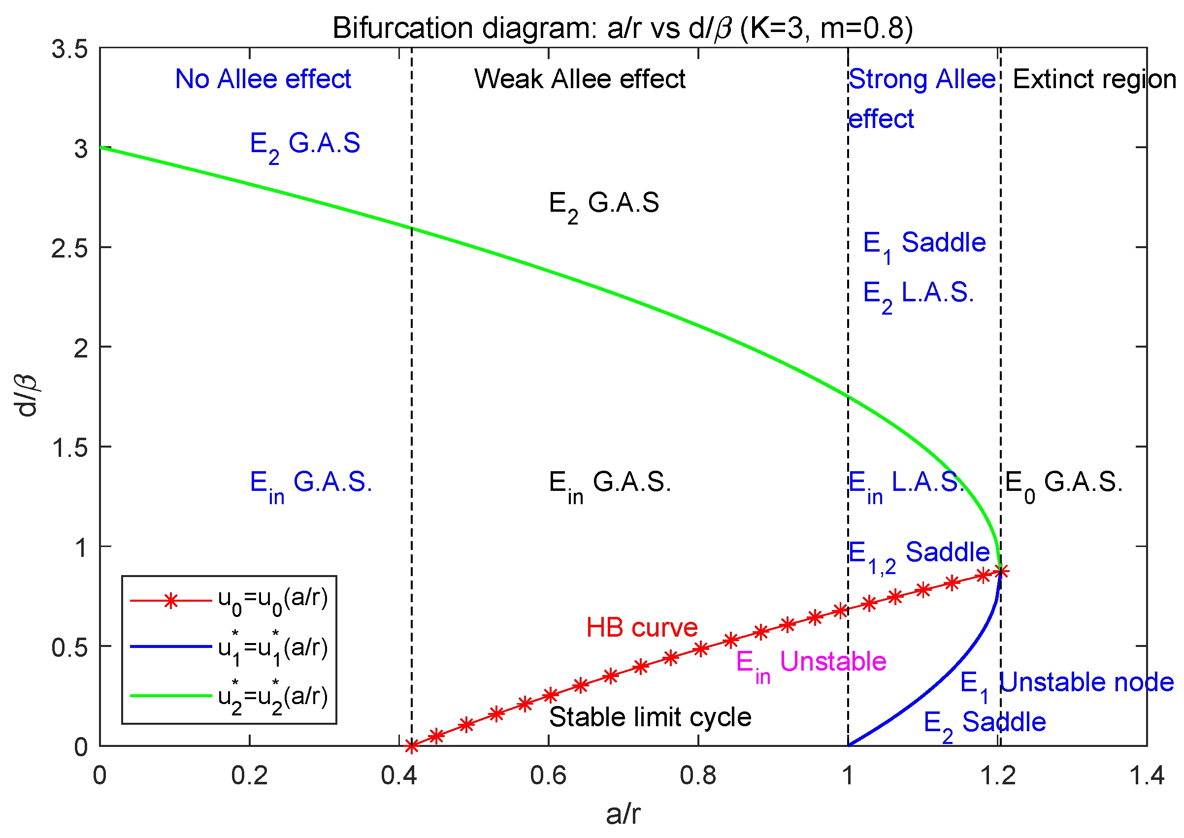
When $\frac{a}{r}>\frac{{(mK+1)}^2}{4mK}=1.2042$, the parameter $\nu =(a,r,m,K)$ lies in the extinct region, i.e., $\nu =(a,r,m,K)\in D_0$; model (2) only has the extinction equilibrium $E_0(0,0)$ which is globally asymptotically stable. In this case, both the predator and prey species will be extinct.

(2)

When $1<\frac{a}{r}<\frac{{(mK+1)}^2}{4mK}=1.2042$, model (2) admits the strong Allee effect. In this case, model (2) has three boundary equilibria $E_i(i=0,1,2)$, where $E_0(0,0)$ is a stable node (see Section 3.3).

(2.1)

Above the green curve (i.e., $\frac{d}{\beta }>u_2^{*}$), model (2) has no positive equilibrium, $E_1$ is a saddle, both $E_0$ and $E_2$ are stable nodes. So, the community cannot be permanent. The prey species may survive but it depends on the initial size of predator and prey (see Figure 3g).

(2.2)

Below the blue curve (i.e., $\frac{d}{\beta }<u_1^{*}$), $E_2(u_2^{*},0)$ is a saddle, $E_1(u_1^{*},0)$ is an unstable node, and $E_0(0,0)$ is globally asymptotically stable. So, two species will be extinct (see Figure 3a).

(2.3)

Between the blue and green curves (i.e., $u_1^{*}<\frac{d}{\beta }<u_2^{*}$), the interior equilibrium $E_{in}(u^{*},v^{*})$ exists, and both $E_1$ and $E_2$ are saddle. Between the red and green curve (i.e., $u_0<\frac{d}{\beta }<u_2^{*}$), $E_{in}$ is locally asymptotically stable; between the blue and red curve (i.e., $u_1^{*}<\frac{d}{\beta }<u_0$), it is unstable; along the red curve (i.e., $\frac{d}{\beta }=u_0$), Hopf bifurcation occurs. The two species may coexist but it depends on their initial population sizes. In this case, model (2) may have the heteroclinic loop connecting $E_1$ and $E_2$ (see Figure 3b–f).

(3)

When $0.425=\frac{1}{mK}<\frac{a}{r}<1$, model (2) has weak Allee effect. In this case, model (2) has two boundary equilibria $E_i(i=0,2)$, where $E_0(0,0)$ is a saddle (see Section 3.4).

(3.1)

Above the green curve (i.e., $\frac{d}{\beta }>u_2^{*}$), model (2) has no positive equilibrium; $E_2$ is globally asymptotically stable; that is, the predator will be extinct while the prey is permanent (see Figure 4d).

(3.2)

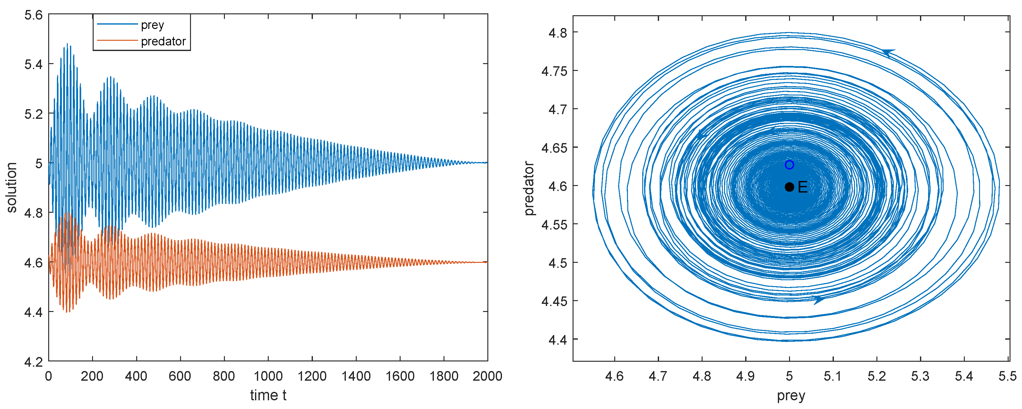
Below the green curve (i.e., $0<\frac{d}{\beta }<u_2^{*}$), the interior equilibrium $E_{in}$ exists, $E_2$ is a saddle. Between the red and green curve (i.e., $u_0<\frac{d}{\beta }<u_2^{*}$), $E_{in}$ is globally asymptotically stable; below the red curve (i.e., $0<\frac{d}{\beta }<u_0$), model (2) has a stable limit cycle surrounding $E_{in}$; along the red curve (i.e., $\frac{d}{\beta }=u_0$), Hopf bifurcation occurs. So, in this case, two species can coexist (see Figure 4a–c).

(4)

When $\frac{a}{r}<\frac{1}{mK}=0.425$, model (2) has no Allee effect. In this case, model (2) has two boundary equilibria $E_i(i=0,2)$, where $E_0(0,0)$ is a saddle (see Section 3.5).

(4.1)

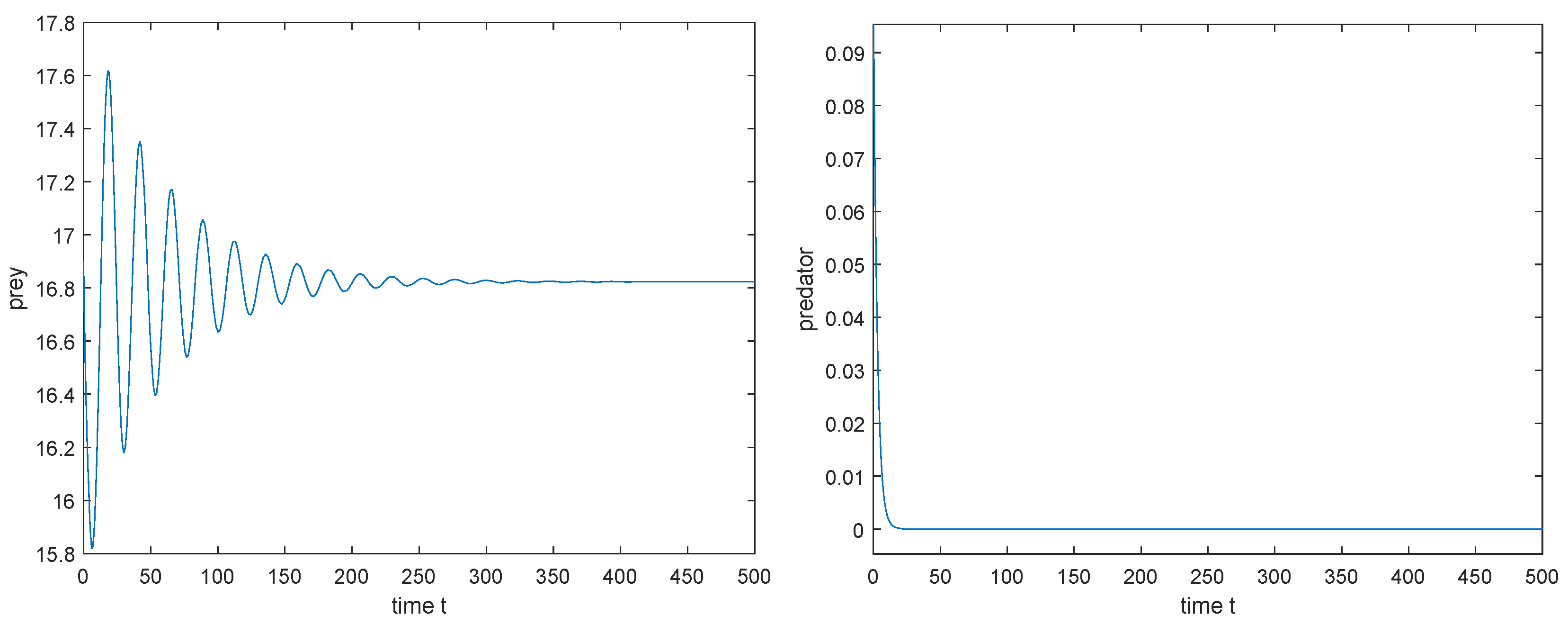
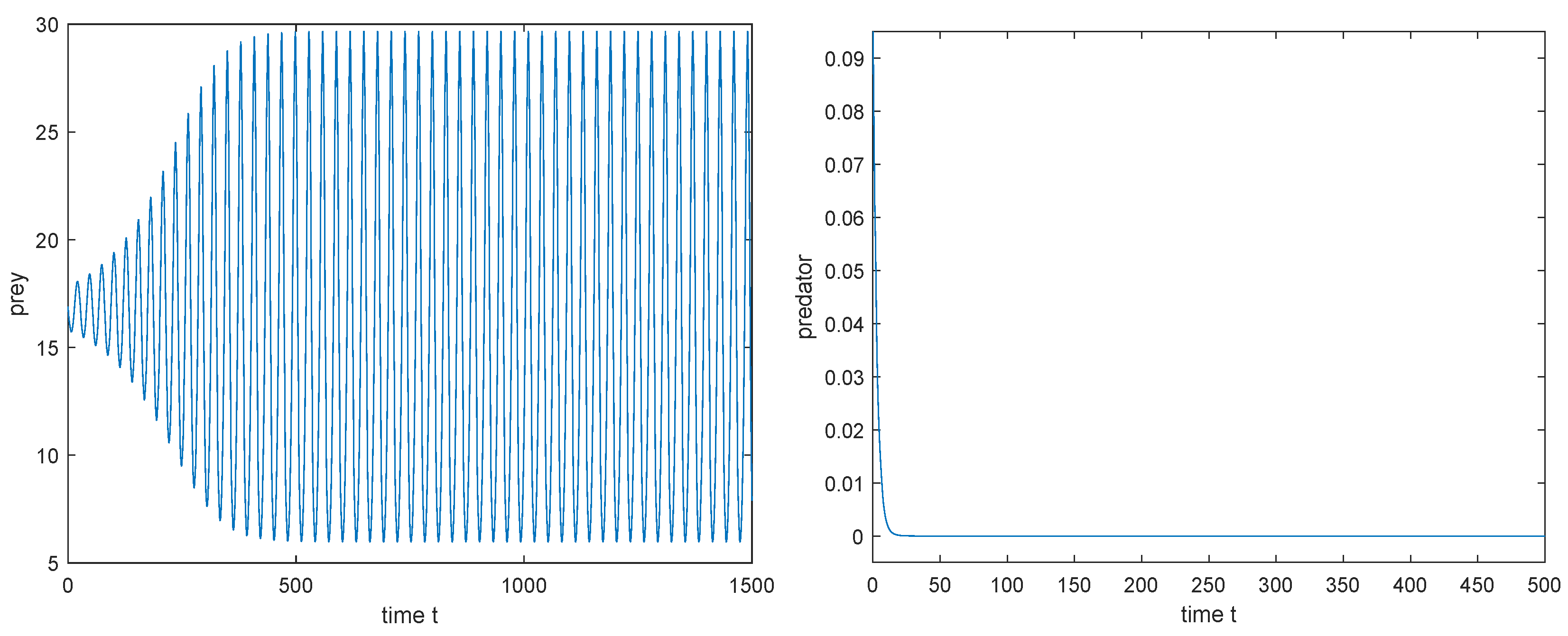
Above the green curve (i.e., $\frac{d}{\beta }>u_2^{*}$), model (2) has no positive equilibrium; $E_2$ is globally asymptotically stable; that is, the predator will be extinct while the prey is permanent.

(4.2)

Below the blue curve (i.e., $0<\frac{d}{\beta }<u_2^{*}$), the interior equilibrium $E_{in}$ exists and is globally asymptotically stable. So, in this case, two species can coexist.

4. The Influence of Delay

In this section, we consider the delayed model (3) and study the Hopf bifurcations caused by the delay.

4.1. Stability and Hopf Bifurcation Induced by Delay

The linear system of (3) with respect to any of its equilibria $(u_{*},v_{*})$ can be expressed as $\dot{Y}\left(t\right)=X_{1}Y\left(t\right)+X_{2}Y(t-\tau )$, where $Y={(U,V)}^T$,

$$\begin{array}{c}\hfill X_1=\left(\begin{array}{cc}r(1-\frac{u_{*}}{K})-\alpha v_{*}-\frac{a}{{(1+m{u}_{*})}^2}& -\alpha u_{*}\\ \beta v_{*}& \beta u_{*}-d\end{array}\right)=\left(\begin{array}{cc}{b}_1\left(u_{*}\right)-\alpha v_{*}& -\alpha u_{*}\\ \beta v_{*}& \beta u_{*}-d\end{array}\right)\end{array}$$

and

$$\begin{array}{c}\hfill X_2=\left(\begin{array}{cc}-\frac{r{u}_{*}}{K}& 0\\ 0& 0\end{array}\right)=\left(\begin{array}{cc}-b_2\left(u_{*}\right)& 0\\ 0& 0\end{array}\right).\end{array}$$

The characteristic equation is given by $|\lambda I-X_1-X_2{e}^{-\lambda \tau }|=0$, i.e.,

$$(\lambda -(b_1\left(u_{*}\right)-\alpha v_{*}))(\lambda -(\beta u_{*}-d))+\alpha \beta u_{*}{v}_{*}+b_2\left(u_{*}\right)(\lambda -(\beta u_{*}-d))e^{-\lambda \tau }=0.$$

(17)

At $E_0(0,0)$, (17) becomes $(\lambda -b_1\left(0\right))(\lambda +d)=0$, where $b_1\left(0\right)=r-a$. Thus, for all $\tau >0$, $E_0(0,0)$ is locally asymptotically stable if $\frac{a}{r}>1$, and unstable if $0<\frac{a}{r}<1$.

At the semi-trivial boundary equilibrium $E_i(u_i^{*},0),i=1,2$, $u_i^{*}$ is given by (8), (17) becomes

$$(\lambda -(\beta u_i^{*}-d))(\lambda -b_1\left(u_i^{*}\right)+b_2\left(u_i^{*}\right)e^{-\lambda \tau })=0,$$

(18)

which gives an eigenvalue ${\lambda }_1=\beta u_i^{*}-d$. Thus, ${\lambda }_1<0$ if and only if $u_i^{*}<\frac{d}{\beta }$. The other eigenvalues are determined by

$$\lambda =b_1\left(u_i^{*}\right)-b_2\left(u_i^{*}\right)e^{-\lambda \tau }.$$

(19)

At $E_1(u_1^{*},0)$, since $b_1\left(u_1^{*}\right)-b_2\left(u_1^{*}\right)=u_1^{*}{H}^{\prime }\left(u_1^{*}\right)>0$ by Lemma 1, we know that (19) has roots with positive real parts for each $\tau >0$ by Theorem 4.7 from Smith [33], which implies that $E_1(u_1^{*},0)$ is always unstable for all $\tau >0$.

At $E_2(u_2^{*},0)$, $b_1\left(u_2^{*}\right)-b_2\left(u_2^{*}\right)=u_1^{*}{H}^{\prime }\left(u_1^{*}\right)<0$ by Lemma 1, then by Theorem 4.7 from Smith [33] there exists a ${\tau }^{*}>0$, which is given by

$${\tau }^{*}=\frac{1}{\sqrt{{\left[b_2\left(u_2^{*}\right)\right]}^2-{\left[b_1\left(u_2^{*}\right)\right]}^2}}arccos\frac{b_1\left(u_2^{*}\right)}{b_2\left(u_2^{*}\right)}.$$

(20)

such that the real parts of all roots of (19) are negative for $\tau \in (0,{\tau }^{*})$, and (19) has roots with positive real parts for each $\tau >{\tau }^{*}$. Therefore, we can conclude that when $u_2^{*}<\frac{d}{\beta }$, $E_2(u_2^{*},0)$ is locally asymptotically stable for $\tau \in (0,{\tau }^{*})$, and unstable for $\tau \in ({\tau }^{*},+\infty )$; when $u_2^{*}>\frac{d}{\beta }$, $E_2(u_2^{*},0)$ is unstable for all $\tau >0$.

Let $u_2^{*}<\frac{d}{\beta }$. Now we show that when $\tau ={\tau }^{*}$, model (3) undergoes the Hopf bifurcation at $E_2(u_2^{*},0)$. As $\tau$ varies, if the stability of $E_2(u_2^{*},0)$ switches at $\tau ={\tau }^{*}$, then the characteristic Equation (18), i.e., the Equation (19), must have a pair of pure conjugate imaginary roots when $\tau ={\tau }^{*}$ (see [33,34]). Let $\lambda =iw(w>0)$ be a root of (18) (i.e., (19)), then we have $sin\left(w\tau \right)=\frac{w}{b_2}$ and $cos\left(w\tau \right)=\frac{b_1}{b_2}$. Thus, one can get the unique critical delay $\tau ={\tau }^{*}$ and the value $w=\sqrt{{\left[b_2\left(u_2^{*}\right)\right]}^2-{\left[b_1\left(u_2^{*}\right)\right]}^2}$. By differentiating (18) with respect to $\tau$, we have

$$\begin{array}{c}\hfill (\lambda -b_1\left(u_2^{*}\right)+b_2\left(u_2^{*}\right)e^{-\lambda \tau })\frac{\mathrm{d}\lambda }{\mathrm{d}\tau }+(\lambda -(\beta u_2^{*}-d))\left((1-\tau b_2\left(u_2^{*}\right)e^{-\lambda \tau })\frac{\mathrm{d}\lambda }{\mathrm{d}\tau }-b_2\left(u_2^{*}\right)\lambda e^{-\lambda \tau }\right)=0.\end{array}$$

At $\lambda =iw$ and $\tau ={\tau }^{*}$, $\lambda -b_1\left(u_2^{*}\right)+b_2\left(u_2^{*}\right)e^{-\lambda \tau }=0$ and $\lambda -(\beta u_2^{*}-d)\ne 0$; thus, we get

$$\begin{array}{c}\hfill \frac{\mathrm{d}\lambda }{\mathrm{d}\tau }{|}_{\lambda =iw}=\frac{i{b}_2\left(u_2^{*}\right)w}{e^{-iw\tau }-b_2\left(u_2^{*}\right)\tau }.\end{array}$$

It follows

$$\begin{array}{c}\hfill \mathrm{Sign}\left(\frac{\mathrm{d}(\Re \lambda )}{\mathrm{d}\tau }{|}_{\lambda =iw}\right)=\mathrm{Sign}\left\{{\left(\frac{\mathrm{d}(\Re \lambda )}{\mathrm{d}\tau }{|}_{\lambda =iw}\right)}^{-1}\right\}=\mathrm{Sign}\left\{\frac{sin\left(w\tau \right)}{b_{2}w}\right\}=\mathrm{Sign}\left\{\frac{1}{b_2^2}\right\}>0.\end{array}$$

This implies that, with increasing $\tau$, all the roots of (19) (and hence (18)) that cross the imaginary axis at $iw$ cross from left to right whenever $\tau ={\tau }^{*}$; therefore, the stability of boundary equilibrium $E_2(u_2^{*},0)$ undergoes a switch from stable to unstable, and the Hopf bifurcation occurs at $E_2(u_2^{*},0)$.

Conclusively, we have the following result.

Theorem 9.

The stability of the delayed model (3) at the boundary equilibria $E_0(0,0)$, $E_1(u_1^{*},0)$ and $E_2(u_2^{*},0)$ is stated as follows.

1.

For all $\tau >0$, $E_0(0,0)$ is locally asymptotically stable if $\frac{a}{r}>1$, and unstable if $0<\frac{a}{r}<1$.

2.

If $E_1(u_1^{*},0)$ exists, it is unstable for all $\tau >0$.

3.

If $E_2(u_2^{*},0)$ exists, then (i) when $u_2^{*}<\frac{d}{\beta }$, there exists a ${\tau }^{*}>0$ such that $E_2(u_2^{*},0)$ is locally asymptotically stable for $\tau \in (0,{\tau }^{*})$, unstable for $\tau \in ({\tau }^{*},+\infty )$, and undergoes Hopf bifurcation at $\tau ={\tau }^{*}$; (ii) when $u_2^{*}>\frac{d}{\beta }$, $E_2(u_2^{*},0)$ is unstable for all $\tau >0$.

At the positive equilibrium $E_{in}(u^{*},v^{*})$, where $u^{*}=\frac{d}{\beta },v^{*}=\frac{1}{\alpha }H\left(u^{*}\right)$, (17) becomes

$$F(\lambda ,\tau )={\lambda }^2-(b_1\left(u^{*}\right)-H\left(u^{*}\right))\lambda +\alpha d{v}^{*}+b_2\left(u^{*}\right)\lambda e^{-\lambda \tau }=0.$$

(21)

Denote ${\tilde{b}}_1\left(u^{*}\right)=b_1\left(u^{*}\right)-H\left(u^{*}\right)$. It is clear that ${\tilde{b}}_1\left(u^{*}\right)=\frac{am{u}^{*}}{{(1+m{u}^{*})}^2}>0$. For convenience, in what follows we write ${\tilde{b}}_1\left(u^{*}\right)$ and $b_2\left(u^{*}\right)$ as ${\tilde{b}}_1$ and $b_2$, respectively.

Let $\lambda =iw(w>0)$ be a root of $F(\lambda ,\tau )=0$; then, we have

$$\left\{\begin{array}{c}-w^2+\alpha d{v}^{*}+b_{2}wsin\left(w\tau \right)=0,\hfill \\ -{\tilde{b}}_{1}w+b_{2}wcos\left(w\tau \right)=0,\hfill \end{array}\right.$$

(22)

which follows

$$w^4-(b_2^2-{\tilde{b}}_1^2+2\alpha d{v}^{*})w^2+{\left(\alpha d{v}^{*}\right)}^2=0.$$

(23)

It is easy to see that (23) has positive roots if and only if

$$\begin{array}{c}\hfill \left\{\begin{array}{c}{b}_2^2-{\tilde{b}}_1^2+2\alpha d{v}^{*}>0,\hfill \\ {\mathsf{\Delta }}_1:=(b_2^2-{\tilde{b}}_1^2)(b_2^2-{\tilde{b}}_1^2+4\alpha d{v}^{*})=(b_2-{\tilde{b}}_1)(b_2+{\tilde{b}}_1)(b_2^2-{\tilde{b}}_1^2+4\alpha d{v}^{*})>0.\hfill \end{array}\right.\end{array}$$

Notice that ${\tilde{b}}_1\left(u^{*}\right)-b_2\left(u^{*}\right)=b_1\left(u^{*}\right)-b_2\left(u^{*}\right)-H\left(u^{*}\right)=u^{*}{H}^{\prime }\left(u^{*}\right)$. Therefore,

• If $b_2<{\tilde{b}}_1$, i.e., $H^{\prime }\left(u^{*}\right)>0$, (23) has no positive root; that is, $F(\lambda ,\tau )=0$ has no purely imaginary root, and hence $E_{in}(u^{*},v^{*})$ is unstable for all $\tau \in [0,\infty )$ since $E_{in}(u^{*},v^{*})$ is unstable when $\tau =0$ by Lemma 2.
• If $b_2>{\tilde{b}}_1$, i.e., $H^{\prime }\left(u^{*}\right)<0$, (23) has two different positive roots $0<w_{-}<w_{+}$, where

  $$w_{\pm }^2=\frac{1}{2}((b_2^2-{\tilde{b}}_1^2+2\alpha d{v}^{*})\pm \sqrt{{\mathsf{\Delta }}_1}).$$

  (24)

Let $b_2\left(u^{*}\right)>{\tilde{b}}_1\left(u^{*}\right)$, i.e., $H^{\prime }\left(u^{*}\right)<0$. Substituting $w_{\pm }^2$ into (22), we get

$$\begin{array}{c}\hfill tan\left(w_{\pm }\tau \right)=\frac{w_{\pm }^2-\alpha d{v}^{*}}{{\tilde{b}}_1{w}_{\pm }}.\end{array}$$

Let ${\theta }_{\pm }=arctan\left(\frac{w_{\pm }^2-\alpha d{v}^{*}}{{\tilde{b}}_1{w}_{\pm }}\right)$. Since

$$\begin{array}{c}\hfill w_{\pm }^2-\alpha d{v}^{*}=\frac{1}{2}(b_2^2-{\tilde{b}}_1^2\pm \sqrt{{\mathsf{\Delta }}_1}),\sqrt{{\mathsf{\Delta }}_1}=\sqrt{(b_2^2-{\tilde{b}}_1^2)(b_2^2-{\tilde{b}}_1^2+4\alpha d{v}^{*})}>b_2^2-{\tilde{b}}_1^2,\end{array}$$

we get $\frac{w_{-}^2-\alpha d{v}^{*}}{{\tilde{b}}_1{w}_{-}}<0<\frac{w_{+}^2-\alpha d{v}^{*}}{{\tilde{b}}_1{w}_{+}}$; that is, $-\frac{\pi }{2}<{\theta }_{-}<0<{\theta }_{+}<\frac{\pi }{2}$. Thus, we obtain the following two sets of values of $\tau$ for which (21) has imaginary roots:

$${\tau }_k^{+}=\frac{{\theta }_{+}+2k\pi }{w_{+}},{\tau }_k^{-}=\frac{{\theta }_{-}+2(k+1)\pi }{w_{-}},k=0,1,2,\cdots .$$

(25)

We need to determine the sign of the derivative of $\Re \lambda \left(\tau \right)$ at the points where $\lambda \left(\tau \right)$ is purely imaginary. From (21), we have

$$\begin{array}{c}\hfill \frac{\mathrm{d}\lambda }{\mathrm{d}\tau }=\frac{b_2{\lambda }^2{e}^{-\lambda \tau }}{2\lambda -{\tilde{b}}_1+b_2{e}^{-\lambda \tau }-b_2\lambda \tau e^{-\lambda \tau }}.\end{array}$$

Then we have

$$\begin{array}{c}\hfill \frac{\mathrm{d}\lambda }{\mathrm{d}\tau }{|}_{\lambda =iw}=\frac{-{\tilde{b}}_1{w}^2+iw(w^2-\alpha d{v}^{*})}{-\tau (w^2-\alpha d{v}^{*})+i(w+\frac{\alpha d{v}^{*}}{w}-{\tilde{b}}_{1}w\tau )}.\end{array}$$

Thus,

$$\begin{array}{c}\hfill \frac{\mathrm{d}(\Re \lambda )}{\mathrm{d}\tau }{|}_{\lambda =iw}=\frac{(w^2-\alpha d{v}^{*})(w^2+\alpha d{v}^{*})}{{\tau }^2{(w^2-\alpha d{v}^{*})}^2+{(w+\frac{\alpha d{v}^{*}}{w}-{\tilde{b}}_{1}w\tau )}^2}.\end{array}$$

Since $w_{+}^2-\alpha d{v}^{*}>0,w_{-}^2-\alpha d{v}^{*}<0$, we get

$$\begin{array}{c}\hfill \frac{\mathrm{d}(\Re \lambda )}{\mathrm{d}\tau }{|}_{\tau ={\tau }_k^{+}}>0,\frac{\mathrm{d}(\Re \lambda )}{\mathrm{d}\tau }{|}_{\tau ={\tau }_k^{-}}<0,k=0,1,2,\cdots .\end{array}$$

This implies that, with increasing $\tau$, all the roots of (21) that cross the imaginary axis at $i{w}_{+}$ cross from left to right whenever $\tau ={\tau }_k^{+}$, and cross at $i{w}_{-}$ from right to left for $\tau ={\tau }_k^{-}$.

By Lemma 2, as $\tau =0$, $E_{in}(u^{*},v^{*})$ is locally asymptotically stable when $H^{\prime }\left(u^{*}\right)<0$ (i.e., $b_2\left(u^{*}\right)>{\tilde{b}}_1\left(u^{*}\right)$). Then it must follow that ${\tau }_0^{+}<{\tau }_0^{-}$. Observe that

$$\begin{array}{c}\hfill {\tau }_{k+1}^{+}-{\tau }_k^{+}=\frac{2\pi }{w^{+}}<\frac{2\pi }{w^{-}}={\tau }_{k+1}^{-}-{\tau }_k^{-}.\end{array}$$

Then there exists a positive integer p such that

$$\begin{array}{c}\hfill 0<{\tau }_0^{+}<{\tau }_0^{-}<{\tau }_1^{+}<{\tau }_1^{-}<\cdots <{\tau }_{p-1}^{+}<{\tau }_{p-1}^{-}<{\tau }_p^{+}<{\tau }_{p+1}^{+}<{\tau }_p^{-}<\cdots .\end{array}$$

It follows that model (3) is locally asymptotically stable at $E_{in}(u^{*},v^{*})$ for $\tau \in (0,{\tau }_0^{+})\cup ({\tau }_0^{-},{\tau }_1^{+})\cup \cdots \cup ({\tau }_{p-1}^{-},{\tau }_p^{+})$, unstable for $\tau \in ({\tau }_0^{+},{\tau }_0^{-})\cup ({\tau }_1^{+},{\tau }_1^{-})\cup \cdots \cup ({\tau }_{p-1}^{+},{\tau }_{p-1}^{-})\cup ({\tau }_p^{+},+\infty )$, and undergoes Hopf-bifurcation at $\tau ={\tau }_k^{\pm }(k=0,1,\cdots ,p-1)$ and $\tau ={\tau }_p^{+}$.

From the above analysis, we have the following result.

Theorem 10.

Assume that $E_{in}(u^{*},v^{*})$ exists.

1.

If $H^{\prime }\left(u^{*}\right)>0$, system (3) is unstable at $E_{in}(u^{*},v^{*})$ for all $\tau \ge 0$.

2.

If $H^{\prime }\left(u^{*}\right)<0$, and there exists a positive integer p such that $0<{\tau }_0^{+}<{\tau }_0^{-}<{\tau }_1^{+}<{\tau }_1^{-}<\cdots <{\tau }_{p-1}^{+}<{\tau }_{p-1}^{-}<{\tau }_p^{+}<{\tau }_{p+1}^{+}<{\tau }_p^{-}<\cdots$, then system (3) is locally asymptotically stable at $E_{in}(u^{*},v^{*})$ for $\tau \in [0,{\tau }_0^{+})\cup ({\tau }_0^{-},{\tau }_1^{+})\cup \cdots \cup ({\tau }_{p-1}^{-},{\tau }_p^{+})$, unstable for $\tau \in ({\tau }_0^{+},{\tau }_0^{-})\cup ({\tau }_1^{+},{\tau }_1^{-})\cup \cdots \cup ({\tau }_{p-1}^{+},{\tau }_{p-1}^{-})\cup ({\tau }_p^{+},+\infty )$, and undergoes Hopf bifurcation at $\tau ={\tau }_k^{\pm }(k=0,1,\cdots ,p-1)$ and $\tau ={\tau }_p^{+}$.

4.2. Direction and the Stability of Hopf-Bifurcating Periodic Solutions

In this subsection, we use the normal form method and the center manifold theory introduced by Hassard et al. [36] to analyze the properties of Hopf bifurcation around $E_{in}$ and $E_2(u_2^{*},0)$, respectively, including the direction of Hopf bifurcation, and the stability and period of the Hopf-bifurcating periodic solutions. These properties are determined by the following three quantities:

$${\mu }_2=-\frac{\Re \left\{\mathfrak{C}\right(0\left)\right\}}{\Re \left\{{\lambda }^{\prime }\left(\overline{\tau }\right)\right\}},{\beta }_2=2\Re \left\{\mathfrak{C}\left(0\right)\right\},T=-\frac{\Im \left\{\mathfrak{C}\left(0\right)\right\}+{\mu }_2\Im \left\{{\lambda }^{\prime }\left(\overline{\tau }\right)\right\}}{w_0\overline{\tau }},$$

(26)

where $\overline{\tau }$ is the critical time delay such that the characteristic equation has the pure conjugate imaginary roots, and

$$\mathfrak{C}\left(0\right)=\frac{i}{2w_0\overline{\tau }}\left(g_{11}{g}_{20}-2{\left|g_{11}\right|}^2-\frac{{\left|g_{02}\right|}^2}{3}\right)+\frac{g_{21}}{2}.$$

(27)

In the three quantities of (26), ${\mu }_2$ determines the direction of Hopf bifurcation, ${\beta }_2$ determines the stability of Hopf-bifurcating periodic solutions, and T determines the period of Hopf-bifurcating periodic solutions. More precisely (see [35]),

(1)

If ${\mu }_2>0$ (resp. ${\mu }_2<0$), then the Hopf bifurcation is supercritical (resp. subcritical).

(2)

If ${\beta }_2<0$ (resp. ${\beta }_2>0$), then the periodic solution is orbitally asymptotically stable (resp. unstable).

(3)

If $T>0$ (resp. $T<0$), then the period of bifurcating periodic solutions increases (resp. decreases) as the bifurcation parameter (delay time $\tau$) keeps away from the critical value.

In order to get the three important quantities of Hopf bifurcation, it is key to compute the coefficients $g_{11},g_{02},g_{20}$ and $g_{21}$. In what follows, we present the computation of these coefficients at the equilibria $E_{in}$ and $E_2(u_2^{*},0)$, respectively. The calculation process is similar to that in many references (see, e.g., [41,42,43,44,45]).

4.2.1. At the Positive Equilibrium $E_{in}$

From Theorem 10, at the positive equilibrium $E_{in}(u^{*},v^{*})$, when $\tau ={\tau }_0^{\pm },{\tau }_1^{\pm },\cdots ,{\tau }_{p-1}^{\pm },{\tau }_p^{+}$, the characteristic Equation (21) has a pair of conjugate pure imaginary roots $\pm i{w}_{\pm }$ given by (24), and model (3) undergoes the Hopf bifurcation. Let $\tilde{\tau }$ be a critical delay value in the set $\{{\tau }_0^{\pm },{\tau }_1^{\pm },\cdots ,{\tau }_{p-1}^{\pm },{\tau }_p^{+}\}$ and $\pm i{w}_0$ be the corresponding conjugate pure imaginary roots of (21). In what follows, we determine the three quantities given in (26) at $E_{in}$.

Let $z_1\left(t\right)=u\left(\tilde{\tau }t\right)-u^{*}$, $z_2\left(t\right)=v\left(\tilde{\tau }t\right)-v^{*}$, $\tau =\tilde{\tau }+\mu$, $\mu \in \mathbb{R}$. Denote $\mathcal{C}=C([-1,0],{\mathbb{R}}_{+}^2)$. Define $L_{\mu }:\mathcal{C}\to {\mathbb{R}}_{+}^2$, $f:\mathbb{R}\times \mathcal{C}\to {\mathbb{R}}_{+}^2$ as follows

$$\begin{array}{c}\hfill L_{\mu }\left(\varphi \right)=(\tilde{\tau }+\mu )B_1\varphi \left(0\right)+(\tilde{\tau }+\mu )B_2\varphi (-1),f(\mu ,\varphi )=(\tilde{\tau }+\mu )M,\varphi ={({\varphi }_1,{\varphi }_2)}^T\in \mathcal{C},\end{array}$$

where

$$\begin{array}{c}\hfill \begin{array}{cc}& B_1=\left(\begin{array}{cc}\frac{am{u}^{*}}{{(1+m{u}^{*})}^2}& -\alpha u^{*}\\ \beta v^{*}& 0\end{array}\right),B_2=\left(\begin{array}{cc}-\frac{r{u}^{*}}{K}& 0\\ 0& 0\end{array}\right),\hfill \\ & M=\left(\begin{array}{c}-\frac{r}{K}{\varphi }_1\left(0\right){\varphi }_1(-1)-\alpha {\varphi }_1\left(0\right){\varphi }_2\left(0\right)+\frac{2am}{{(1+m{u}^{*})}^3}{\varphi }_1^2\left(0\right)\\ \beta {\varphi }_1\left(0\right){\varphi }_2\left(0\right)\end{array}\right).\hfill \end{array}\end{array}$$

Then model (3) can be written as the following functional differential equation

$$\dot{z}\left(t\right)=L_{\mu }\left(z_t\right)+f(\mu ,z_t),z\left(t\right)={(z_1\left(t\right),z_2\left(t\right))}^T\in {\mathbb{R}}_{+}^2.$$

(28)

By the Riesz representation theorem, there is a matrix function $\eta (\theta ,\mu )$ of bounded variation for $\theta \in [-1,0]$, such that $L_{\mu }\left(\varphi \right)={\int }_{-1}^0\mathrm{d}\eta (\theta ,\mu )\varphi \left(\theta \right)$. We choose $\eta (\theta ,\mu )=(\tilde{\tau }+\mu )B_1\delta \left(\theta \right)-(\tilde{\tau }+\mu )B_2\delta (\theta +1)$, where

$$\begin{array}{c}\hfill \delta \left(\theta \right)=\left\{\begin{array}{cc}& 1,\theta =0,\hfill \\ & 0,\theta \ne 0.\hfill \end{array}\right.\end{array}$$

For $\varphi \in C^1([-1,0],{\mathbb{R}}_{+}^2)$, define the operators

$$A\left(\mu \right)\varphi \left(\theta \right)=\left\{\begin{array}{cc}\hfill \frac{\mathrm{d}\varphi \left(\theta \right)}{\mathrm{d}\theta },& \theta \in [-1,0),\hfill \\ \hfill {\int }_{-1}^0\mathrm{d}\eta (\xi ,\mu )\varphi \left(\xi \right),& \theta =0,\hfill \end{array}\right.$$

(29)

and

$$\begin{array}{c}\hfill R\left(\mu \right)\varphi \left(\theta \right)=\left\{\begin{array}{cc}\hfill 0,& \theta \in [-1,0),\hfill \\ \hfill f(\mu ,\varphi ),& \theta =0.\hfill \end{array}\right.\end{array}$$

Then (28) is equivalent to

$${\dot{z}}_t=A\left(\mu \right)z_t+R\left(\mu \right)z_t,$$

(30)

where $z_t\left(\theta \right)=z(t+\theta )$ for $\theta \in [-1,0]$.

For $\psi \in C^1([0,1],{\left({\mathbb{R}}_{+}^2\right)}^{*})$, define the operator

$$\begin{array}{c}\hfill A^{*}\psi \left(s\right)=\left\{\begin{array}{cc}\hfill -\frac{\mathrm{d}\psi \left(s\right)}{\mathrm{d}s},& s\in (0,1],\hfill \\ \hfill {\int }_{-1}^0\psi (-\xi )\mathrm{d}{\eta }^T(\xi ,0),& s=0,\hfill \end{array}\right.\end{array}$$

and a bilinear inner product

$$⟨\psi \left(s\right),\varphi \left(\theta \right)⟩=\overline{\psi }\left(0\right)\varphi \left(0\right)-{\int }_{\theta =-1}^0{\int }_{\xi =0}^{\theta }\overline{\psi }(\xi -\theta )\mathrm{d}\eta \left(\theta \right)\varphi \left(\xi \right)\mathrm{d}\xi ,$$

(31)

where $\eta \left(\theta \right)=\eta (\theta ,0)$. Then $A\left(0\right)$ and $A^{*}$ are adjoint operators. According to the previous calculation, we know that $\pm i{w}_0\tilde{\tau }$ are the eigenvalues of $A\left(0\right)$, so $\pm i{w}_0\tilde{\tau }$ are also the eigenvalues of $A^{*}$.

Suppose that $q\left(\theta \right)={(1,p)}^T{e}^{i{w}_0\tilde{\tau }\theta }$ and $q^{*}\left(s\right)=k(1,p^{*})e^{i{w}_0\tilde{\tau }s}$ are the eigenvectors of $A\left(0\right)$ and $A^{*}$ corresponding to $i{w}_0\tilde{\tau }$ and $-i{w}_0\tilde{\tau }$, respectively. Then $A\left(0\right)q\left(\theta \right)=i{w}_0\tilde{\tau }q\left(\theta \right)$ and $A^{*}{q}^{*}\left(s\right)=-i{w}_0\tilde{\tau }{q}^{*}\left(s\right)$. With the definition (29) of $A\left(0\right)$, we get

$$\begin{array}{c}\hfill \tilde{\tau }\left(\begin{array}{cc}-\frac{am{u}^{*}}{{(1+m{u}^{*})}^2}+\frac{r{u}^{*}}{K}{e}^{-i{w}_0\tilde{\tau }}+i{w}_0& \alpha u^{*}\\ -\beta v^{*}& i{w}_0\end{array}\right)q\left(0\right)=\left(\begin{array}{c}0\\ 0\end{array}\right),\end{array}$$

and then we have $q\left(0\right)={(1,\frac{\beta v^{*}}{i{w}_0})}^T$, i.e., $q\left(\theta \right)={(1,\frac{\beta v^{*}}{i{w}_0})}^T{e}^{i{w}_0\tilde{\tau }\theta }$.

Similarly, we can get $q^{*}\left(s\right)=k(1,-\frac{\beta v^{*}}{i{w}_0})e^{i{w}_0\tilde{\tau }s}$. Next, we need to select k so that $⟨q^{*}\left(s\right),q\left(\theta \right)⟩=1$, $⟨q^{*}\left(s\right),\overline{q}\left(\theta \right)⟩=0$. From (31), we have

$$\begin{array}{c}\hfill \begin{array}{cc}\hfill ⟨q^{*}\left(s\right),q\left(\theta \right)⟩& =\overline{k}(1,{\overline{p}}^{*}){(1,p)}^T-{\int }_{\theta =-1}^0{\int }_{\xi =0}^{\theta }\overline{k}(1,{\overline{p}}^{*})e^{-i{w}_0\tilde{\tau }(\xi -\theta )}\mathrm{d}\eta \left(\theta \right){(1,p)}^T{e}^{i{w}_0\tilde{\tau }\xi }\mathrm{d}\xi \hfill \\ & =\overline{k}\left[1+{\overline{p}}^{*}p-{\int }_{-1}^0(1,{\overline{p}}^{*})\theta e^{i{w}_0\tilde{\tau }\theta }\mathrm{d}\eta \left(\theta \right){(1,p)}^T\right]\hfill \\ & =\overline{k}\left[1+\frac{{\left(\beta v^{*}\right)}^2}{w_0^2}-\frac{r{u}^{*}\tilde{\tau }}{K}{e}^{-i{w}_0\tilde{\tau }}\right].\hfill \end{array}\end{array}$$

Thus, $k={\left(1+\frac{{\left(\beta v^{*}\right)}^2}{w_0^2}-\frac{r{u}^{*}\tilde{\tau }}{K}{e}^{i{w}_0\tilde{\tau }}\right)}^{-1}$.

Now, by the ideas in Hassard et al. [36], we calculate the coordinates to describe the center manifold ${\mathbf{C}}_0$ at $\mu =0$. For this purpose, let $z_t$ be the solution of Equation (28) when $\mu =0$, and define

$$Z\left(t\right)=⟨q^{*},z_t⟩,W(t,\theta )=z_t\left(\theta \right)-2\Re \left\{Z\left(t\right)q\left(\theta \right)\right\},$$

(32)

on the center manifold ${\mathbf{C}}_0$, we have

$$\begin{array}{c}\hfill W(t,\theta )=W(Z\left(t\right),\overline{Z}\left(t\right),\theta ),\end{array}$$

where $W(Z,\overline{Z},\theta )=W_{20}\left(\theta \right)\frac{Z^2}{2}+W_{11}\left(\theta \right)Z\overline{Z}+W_{02}\left(\theta \right)\frac{{\overline{Z}}^2}{2}+\cdots$, Z and $\overline{Z}$ are the local coordinates of ${\mathbf{C}}_0$ in the direction of $q^{*}$ and ${\overline{q}}^{*}$.

Note that W is real if and only if $z_t$ is real. Here we only consider real solutions. For the solution $z_t\in {\mathbf{C}}_0$ of Equation (28), when $\mu =0$, we have

$$\begin{array}{c}\hfill \begin{array}{cc}\hfill \dot{Z}\left(t\right)& =i{w}_0\tilde{\tau }Z+⟨{\overline{q}}^{*}\left(\theta \right),f(0,W(Z,\overline{Z},\theta )+2\Re \left\{Zq\left(\theta \right)\right\})⟩\hfill \\ & =i{w}_0\tilde{\tau }Z+{\overline{q}}^{*}\left(0\right)f(0,W(Z,\overline{Z},0)+2\Re \left\{Zq\left(0\right)\right\})\hfill \\ & =i{w}_0\tilde{\tau }Z+{\overline{q}}^{*}\left(0\right)f_0(Z,\overline{Z})\hfill \\ & =i{w}_0\tilde{\tau }Z+g(Z,\overline{Z}),\hfill \end{array}\end{array}$$

where $g(Z,\overline{Z})={\overline{q}}^{*}\left(0\right)f_0(Z,\overline{Z})=g_{20}\frac{Z^2}{2}+g_{11}Z\overline{Z}+g_{02}\frac{{\overline{Z}}^2}{2}+g_{21}\frac{Z^2\overline{Z}}{2}+\cdots$.

From (32), we have $z_t\left(\theta \right)={(z_{1t}\left(\theta \right),z_{2t}\left(\theta \right))}^T=W(t,\theta )+Zq\left(\theta \right)+\overline{Z}\overline{q}\left(\theta \right)$. Combined with the definitions of W and $q\left(\theta \right)$, the following expressions can be obtained

$$\begin{array}{c}\hfill \begin{array}{cc}\hfill z_{1t}\left(0\right)& =Z+\overline{Z}+W_{20}^{\left(1\right)}\left(0\right)\frac{Z^2}{2}+W_{11}^{\left(1\right)}\left(0\right)Z\overline{Z}+W_{02}^{\left(1\right)}\left(0\right)\frac{{\overline{Z}}^2}{2}+O\left(\right|(Z,\overline{Z}){|}^3),\hfill \\ \hfill z_{2t}\left(0\right)& =Zp+\overline{Z}\overline{p}+W_{20}^{\left(2\right)}\left(0\right)\frac{Z^2}{2}+W_{11}^{\left(2\right)}\left(0\right)Z\overline{Z}+W_{02}^{\left(2\right)}\left(0\right)\frac{{\overline{Z}}^2}{2}+O\left(\right|(Z,\overline{Z}){|}^3),\hfill \\ \hfill z_{1t}(-1)& =Z{e}^{-i{w}_0\tilde{\tau }}+\overline{Z}{e}^{i{w}_0\tilde{\tau }}+W_{20}^{\left(1\right)}(-1)\frac{Z^2}{2}+W_{11}^{\left(1\right)}(-1)Z\overline{Z}+W_{02}^{\left(1\right)}(-1)\frac{{\overline{Z}}^2}{2}+O\left(\right|(Z,\overline{Z}){|}^3),\hfill \\ \hfill z_{2t}(-1)& =Zp{e}^{-i{w}_0\tilde{\tau }}+\overline{Z}\overline{p}{e}^{i{w}_0\tilde{\tau }}+W_{20}^{\left(2\right)}(-1)\frac{Z^2}{2}+W_{11}^{\left(2\right)}(-1)Z\overline{Z}+W_{02}^{\left(2\right)}(-1)\frac{{\overline{Z}}^2}{2}+O\left(\right|(Z,\overline{Z}){|}^3).\hfill \end{array}\end{array}$$

By the definitions of $q^{*}$ and $f_0(Z,\overline{Z})$, $g(Z,\overline{Z})$ can be rewritten as

$$\begin{array}{c}\hfill \begin{array}{cc}\hfill g(Z,\overline{Z})=& {\overline{q}}^{*}\left(0\right)f_0(Z,\overline{Z})\hfill \\ \hfill =& \overline{k}\tilde{\tau }(1,p^{*})\left(\begin{array}{c}-\frac{r}{K}{z}_{1t}\left(0\right)z_{1t}(-1)-\alpha z_{1t}\left(0\right)z_{2t}\left(0\right)+\frac{2am}{{(1+m{u}^{*})}^3}{z}_{1t}^2\left(0\right)\\ \beta z_{1t}\left(0\right)z_{2t}\left(0\right)\end{array}\right)\hfill \\ \hfill =& \overline{k}\tilde{\tau }\{Z^2[-\frac{r}{K}{e}^{-i{w}_0\tilde{\tau }}+p(\beta p^{*}-\alpha )+\frac{2am}{{(1+m{u}^{*})}^3}]\hfill \\ & +{\overline{Z}}^2[-\frac{r}{K}{e}^{i{w}_0\tilde{\tau }}+\overline{p}(\beta p^{*}-\alpha )+\frac{2am}{{(1+m{u}^{*})}^3}]\hfill \\ & +Z\overline{Z}[-\frac{r}{K}(e^{i{w}_0\tilde{\tau }}+e^{-i{w}_0\tilde{\tau }})+\frac{4am}{{(1+m{u}^{*})}^3}]\hfill \\ & +Z^2\overline{Z}[-\frac{r}{K}(W_{11}^{\left(1\right)}(-1)+\frac{W_{20}^{\left(1\right)}(-1)}{2}+\frac{W_{20}^{\left(1\right)}\left(0\right)}{2}{e}^{i{w}_0\tilde{\tau }}+W_{11}^{\left(1\right)}\left(0\right)e^{-i{w}_0\tilde{\tau }})\hfill \\ & +(\beta p^{*}-\alpha )(W_{11}^{\left(2\right)}\left(0\right)+\frac{W_{20}^{\left(2\right)}\left(0\right)}{2}+\frac{W_{20}^{\left(1\right)}\left(0\right)}{2}\overline{p}+W_{11}^{\left(1\right)}\left(0\right)p)\hfill \\ & +\frac{2am}{{(1+m{u}^{*})}^3}(2W_{11}^{\left(1\right)}\left(0\right)+W_{20}^{\left(1\right)}\left(0\right))]+\cdots \}.\hfill \end{array}\end{array}$$

So, we get the following coefficients:

$$\begin{array}{cc}\hfill g_{20}=& 2\overline{k}\tilde{\tau }[-\frac{r}{K}{e}^{-i{w}_0\tilde{\tau }}+p(\beta p^{*}-\alpha )+\frac{2am}{{(1+m{u}^{*})}^3}],\hfill \\ \hfill g_{11}=& \overline{k}\tilde{\tau }[-\frac{r}{K}(e^{i{w}_0\tilde{\tau }}+e^{-i{w}_0\tilde{\tau }})+\frac{4am}{{(1+m{u}^{*})}^3}],\hfill \\ \hfill g_{02}=& 2\overline{k}\tilde{\tau }[-\frac{r}{K}{e}^{i{w}_0\tilde{\tau }}+\overline{p}(\beta p^{*}-\alpha )+\frac{2am}{{(1+m{u}^{*})}^3}],\hfill \\ \hfill g_{21}=& 2\overline{k}\tilde{\tau }[-\frac{r}{K}(W_{11}^{\left(1\right)}(-1)+\frac{W_{20}^{\left(1\right)}(-1)}{2}+\frac{W_{20}^{\left(1\right)}\left(0\right)}{2}{e}^{i{w}_0\tilde{\tau }}+W_{11}^{\left(1\right)}\left(0\right)e^{-i{w}_0\tilde{\tau }})\hfill \\ \hfill & +(\beta p^{*}-\alpha )(W_{11}^{\left(2\right)}\left(0\right)+\frac{W_{20}^{\left(2\right)}\left(0\right)}{2}+\frac{W_{20}^{\left(1\right)}\left(0\right)}{2}\overline{p}+W_{11}^{\left(1\right)}\left(0\right)p)\hfill \\ \hfill & +\frac{2am}{{(1+m{u}^{*})}^3}(2W_{11}^{\left(1\right)}\left(0\right)+W_{20}^{\left(1\right)}\left(0\right))].\hfill \end{array}$$

(33)

In order to get $g_{21}$, we still need to compute $W_{11}\left(\theta \right)$ and $W_{20}\left(\theta \right)$. From (30) and (32), we have

$$\begin{array}{cc}\hfill \dot{W}& ={\dot{z}}_t-\dot{Z}q-\dot{\overline{Z}}\overline{q}\hfill \\ \hfill & =\left\{\begin{array}{cc}\hfill AW-2\Re \left\{{\overline{q}}^{*}\left(0\right)f_{0}q\left(\theta \right)\right\},& \theta \in [-1,0),\hfill \\ \hfill AW-2\Re \left\{{\overline{q}}^{*}\left(0\right)f_{0}q\left(\theta \right)\right\}+f_0,& \theta =0,\hfill \end{array}\right.\hfill \\ \hfill & =AW+G(Z,\overline{Z},\theta ),\hfill \end{array}$$

(34)

where $G(Z,\overline{Z},\theta )=G_{20}\left(\theta \right)\frac{Z^2}{2}+G_{11}\left(\theta \right)Z\overline{Z}+G_{02}\left(\theta \right)\frac{{\overline{Z}}^2}{2}+\cdots$. Hence, we have

$$(A-2i{w}_0\tilde{\tau }I)W_{20}\left(\theta \right)=-G_{20}\left(\theta \right),A{W}_{11}\left(\theta \right)=-G_{11}\left(\theta \right),\cdots .$$

(35)

From (34), we know that for $\theta \in [-1,0)$,

$$\begin{array}{c}\hfill G(Z,\overline{Z},\theta )=-{\overline{q}}^{*}\left(0\right)f_{0}q\left(\theta \right)-q^{*}\left(0\right){\overline{f}}_0\overline{q}\left(\theta \right)=-gq\left(\theta \right)-\overline{g}\overline{q}\left(\theta \right).\end{array}$$

By comparing the coefficients, we get

$$\begin{array}{c}\hfill G_{20}\left(\theta \right)=-g_{20}q\left(\theta \right)-{\overline{g}}_{02}\overline{q}\left(\theta \right),G_{11}\left(\theta \right)=-g_{11}q\left(\theta \right)-{\overline{g}}_{11}\overline{q}\left(\theta \right).\end{array}$$

Combining the definition of A, we obtain

$$\begin{array}{c}\hfill {\dot{W}}_{20}\left(\theta \right)=2i{w}_0\tilde{\tau }{W}_{20}\left(\theta \right)+g_{20}q\left(\theta \right)+{\overline{g}}_{02}\overline{q}\left(\theta \right),{\dot{W}}_{11}\left(\theta \right)=g_{11}q\left(\theta \right)+{\overline{g}}_{11}\overline{q}\left(\theta \right).\end{array}$$

Since $q\left(\theta \right)={(1,p)}^T{e}^{i{w}_0\tilde{\tau }\theta }$, we have

$$\begin{array}{cc}\hfill W_{20}\left(\theta \right)& =\frac{i{g}_{20}}{w_0\tilde{\tau }}q\left(0\right)e^{i{w}_0\tilde{\tau }\theta }+\frac{i{\overline{g}}_{02}}{3w_0\tilde{\tau }}\overline{q}\left(0\right)e^{-i{w}_0\tilde{\tau }\theta }+e_1{e}^{2i{w}_0\tilde{\tau }\theta },\hfill \\ \hfill W_{11}\left(\theta \right)& =-\frac{i{g}_{11}}{w_0\tilde{\tau }}q\left(0\right)e^{i{w}_0\tilde{\tau }\theta }+\frac{i{\overline{g}}_{11}}{w_0\tilde{\tau }}\overline{q}\left(0\right)e^{-i{w}_0\tilde{\tau }\theta }+e_2,\hfill \end{array}$$

(36)

where $e_1={(e_1^{\left(1\right)},e_1^{\left(2\right)})}^T,e_2={(e_2^{\left(1\right)},e_2^{\left(2\right)})}^T\in {\mathbb{R}}_{+}^2$ are constant vectors to be determined. From (29) and (35), we have

$$\begin{array}{cc}\hfill A\left(0\right)W_{20}\left(0\right)& ={\int }_{-1}^0\mathrm{d}\eta (\xi ,0)W_{20}\left(\xi \right)=2i{w}_0\tilde{\tau }{W}_{20}\left(0\right)-G_{20}\left(0\right),\hfill \\ \hfill A\left(0\right)W_{11}\left(0\right)& ={\int }_{-1}^0\mathrm{d}\eta (\xi ,0)W_{11}\left(\xi \right)=-G_{11}\left(0\right).\hfill \end{array}$$

(37)

From (35), we get

$$\begin{array}{cc}\hfill G_{20}\left(0\right)& =-g_{20}q\left(0\right)-{\overline{g}}_{02}\overline{q}\left(0\right)+2\tilde{\tau }\left(\begin{array}{c}-\frac{r}{K}{e}^{-i{w}_0\tilde{\tau }}-\alpha p+\frac{2am}{{(1+m{u}^{*})}^3}\\ \beta p\end{array}\right),\hfill \\ \hfill G_{11}\left(0\right)& =-g_{11}q\left(0\right)-{\overline{g}}_{11}\overline{q}\left(0\right)+\tilde{\tau }\left(\begin{array}{c}-\frac{r}{K}(e^{-i{w}_0\tilde{\tau }}+e^{i{w}_0\tilde{\tau }})+\frac{4am}{{(1+m{u}^{*})}^3}\\ 0\end{array}\right).\hfill \end{array}$$

(38)

Since $A\left(0\right)q\left(0\right)={\int }_{-1}^0{e}^{i{w}_0\tilde{\tau }\xi }\mathrm{d}\eta (\xi ,0)q\left(0\right)$, we have

$$\begin{array}{c}\hfill \left[i{w}_0\tilde{\tau }I-{\int }_{-1}^0{e}^{i{w}_0\tilde{\tau }\xi }\mathrm{d}\eta (\xi ,0)\right]q\left(0\right)=0,\left[-i{w}_0\tilde{\tau }I-{\int }_{-1}^0{e}^{-i{w}_0\tilde{\tau }\xi }\mathrm{d}\eta (\xi ,0)\right]\overline{q}\left(0\right)=0.\end{array}$$

Substituting (36) and (38) into (37), we get

$$\begin{array}{c}\hfill \begin{array}{cc}\hfill \left(\begin{array}{cc}2i{w}_0-\frac{am{u}^{*}}{{(1+m{u}^{*})}^2}+\frac{r{u}^{*}}{K}{e}^{-2i{w}_0\tilde{\tau }}& \alpha u^{*}\\ -\beta v^{*}& 2i{w}_0\end{array}\right)\left(\begin{array}{c}{e}_1^{\left(1\right)}\\ e_1^{\left(2\right)}\end{array}\right)& =2\left(\begin{array}{c}-\frac{r}{K}{e}^{-i{w}_0\tilde{\tau }}-\alpha p+\frac{2am}{{(1+m{u}^{*})}^3}\\ \beta p\end{array}\right),\hfill \\ \hfill \left(\begin{array}{cc}\frac{am{u}^{*}}{{(1+m{u}^{*})}^2}-\frac{r{u}^{*}}{K}& -\alpha u^{*}\\ \beta v^{*}& 0\end{array}\right)\left(\begin{array}{c}{e}_2^{\left(1\right)}\\ e_2^{\left(2\right)}\end{array}\right)& =\left(\begin{array}{c}\frac{r}{K}(e^{i{w}_0\tilde{\tau }}+e^{-i{w}_0\tilde{\tau }})-\frac{4am}{{(1+m{u}^{*})}^3}\\ 0\end{array}\right).\hfill \end{array}\end{array}$$

By these two equations, we get

$$\begin{array}{cc}\hfill e_1^{\left(1\right)}& =\frac{2}{\left|D_1\right|}\left|\begin{array}{cc}-\frac{r}{K}{e}^{-i{w}_0\tilde{\tau }}-\alpha p+\frac{2am}{{(1+m{u}^{*})}^3}& \alpha u^{*}\\ \beta p& 2i{w}_0\end{array}\right|,\hfill \\ \hfill e_1^{\left(2\right)}& =\frac{2}{\left|D_1\right|}\left|\begin{array}{cc}2i{w}_0-\frac{am{u}^{*}}{{(1+m{u}^{*})}^2}+\frac{r{u}^{*}}{K}{e}^{-2i{w}_0\tilde{\tau }}& -\frac{r}{K}{e}^{-i{w}_0\tilde{\tau }}-\alpha p+\frac{2am}{{(1+m{u}^{*})}^3}\\ -\beta v^{*}& \beta p\end{array}\right|,\hfill \\ \hfill e_2^{\left(1\right)}& =\frac{1}{\left|D_2\right|}\left|\begin{array}{cc}\frac{r}{K}(e^{i{w}_0\tilde{\tau }}+e^{-i{w}_0\tilde{\tau }})-\frac{4am}{{(1+m{u}^{*})}^3}& -\alpha u^{*}\\ 0& 0\end{array}\right|=0,\hfill \\ \hfill e_2^{\left(2\right)}& =\frac{1}{\left|D_2\right|}\left|\begin{array}{cc}\frac{am{u}^{*}}{{(1+m{u}^{*})}^2}-\frac{r{u}^{*}}{K}& \frac{r}{K}(e^{i{w}_0\tilde{\tau }}+e^{-i{w}_0\tilde{\tau }})-\frac{4am}{{(1+m{u}^{*})}^3}\\ \beta v^{*}& 0\end{array}\right|,\hfill \end{array}$$

(39)

where

$$\begin{array}{c}\hfill D_1=\left(\begin{array}{cc}2i{w}_0-\frac{am{u}^{*}}{{(1+m{u}^{*})}^2}+\frac{r{u}^{*}}{K}{e}^{-2i{w}_0\tilde{\tau }}& \alpha u^{*}\\ -\beta v^{*}& 2i{w}_0\end{array}\right),D_2=\left(\begin{array}{cc}\frac{am{u}^{*}}{{(1+m{u}^{*})}^2}-\frac{r{u}^{*}}{K}& -\alpha u^{*}\\ \beta v^{*}& 0\end{array}\right).\end{array}$$

Thus, by (33), (36) and (39), the coefficients $g_{11},g_{02},g_{20}$ and $g_{21}$ can be computed and hence the three quantities (26) of Hopf bifurcation at $E_{in}$ can be determined.

For example, we take the following parameters:

$$r=1.2,K=45,a=1.25,m=1.5,\alpha =0.2,\beta =0.04,d=0.2.$$

This set of parameters implies that model (3) has a strong Allee effect since $1<\frac{a}{r}<\frac{{(mK+1)}^2}{4mK}$. One can get the positive equilibrium $E_{in}(u^{*},v^{*})=(5,4.598)$, which is locally asymptotically stable for model (2) without delay since $H^{\prime }\left(u^{*}\right)\approx -0.00062<0$ by Lemma 2. For the delayed model (3), by (25), the critical delay values are computed as follows:

$${\tau }_0^{+}=0.5222,{\tau }_0^{-}=14.6232,{\tau }_1^{+}=14.6586,{\tau }_1^{-}=29.8073,{\tau }_2^{+}=28.7949,{\tau }_2^{-}=44.9915,\cdots .$$

So, we have

$$0<{\tau }_0^{+}<{\tau }_0^{-}<{\tau }_1^{+}<{\tau }_2^{+}<{\tau }_1^{-}<\cdots .$$

From Theorem 10, we know that as $\tau$ is increasing, the stability of $E_{in}(u^{*},v^{*})=(5,4.598)$ switches twice and $E_{in}$ is locally asymptotically stable for $\tau \in [0,{\tau }_0^{+})\cup ({\tau }_0^{-},{\tau }_1^{+})$ and unstable for $\tau \in ({\tau }_0^{+},{\tau }_0^{-})\cup ({\tau }_1^{+},\infty )$, while model (3) undergoes the Hopf bifurcation at $E_{in}$ when $\tau$ takes ${\tau }_0^{+}=0.5222,{\tau }_0^{-}=14.6232$ and ${\tau }_1^{+}=14.6586$, respectively; see Figure 6, Figure 7, Figure 8, Figure 9, Figure 10, Figure 11 and Figure 12, in which the dynamics of (3) are presented as $\tau$ is increasing.

Figure 6. $\tau =0.3\in [0,{\tau }_0^{+})=[0,0.5222)$, $E_{in}$ is locally asymptotically stable. The initial value: $({\varphi }_1,{\varphi }_2)=(5,4.2)$.

Figure 7. $\tau ={\tau }_0^{+}=0.5222$, the subcritical Hopf bifurcation occurs at $E_{in}$. The initial value: $({\varphi }_1,{\varphi }_2)=(5,4.2)$.

Figure 8. $\tau =2.7\in ({\tau }_0^{+},{\tau }_0^{-})=(0.5222,14.6232)$, $E_{in}$ is unstable. The initial value is $({\varphi }_1,{\varphi }_2)=(5,4.59)$.

Figure 9. $\tau ={\tau }_0^{-}=14.6232$, the subcritical Hopf bifurcation occurs at $E_{in}$. Initial value: $({\varphi }_1,{\varphi }_2)=(5,4.586)$.

Figure 10. $\tau =14.63\in ({\tau }_0^{-},{\tau }_1^{+})=(14.6232,14.6586)$, $E_{in}$ is locally asymptotically stable. Initial value: $({\varphi }_1,{\varphi }_2)=(5,4.627)$.

Figure 11. $\tau ={\tau }_1^{+}=14.6586$, the supercritical Hopf bifurcation occurs at $E_{in}$. Initial value: $({\varphi }_1,{\varphi }_2)=(5,4.586)$.

Figure 12. $\tau =16\in ({\tau }_1^{+},\infty )=(14.6586,\infty )$, $E_{in}$ is unstable. Initial value: $({\varphi }_1,{\varphi }_2)=(5,4.598)$.

1. Taking $\tau =0.3\in [0,{\tau }_0^{+})=[0,0.5222)$, then $E_{in}$ is locally asymptotically stable (see Figure 6), which implies that both the predator and prey can coexist.

2. Taking $\tau$ as the Hopf bifurcation value $\tau ={\tau }_0^{+}=0.5222$, we have the three quantities (26) of Hopf bifurcation: ${\mu }_2=-0.3558,{\beta }_2=0.0054,T=0.0598$. Thus, the Hopf bifurcation is subcritical since ${\mu }_2<0$ and the periodic Hopf orbit is unstable since ${\beta }_2>0$ (see Figure 7).

3. Taking $\tau =2.7\in ({\tau }_0^{+},{\tau }_0^{-})=(0.5222,14.6232)$, $E_{in}$ is unstable (see Figure 8).

4. Choosing $\tau$ as the Hopf bifurcation value $\tau ={\tau }_0^{-}=14.6232$, we have ${\mu }_2=-0.2958$, ${\beta }_2=-0.067,T=-0.0274$, which implies that the Hopf bifurcation is subcritical and the periodic Hopf orbit is asymptotically stable (see Figure 9).

5. Taking $\tau =14.63\in ({\tau }_0^{-},{\tau }_1^{+})=(14.6232,14.6586)$, $E_{in}$ is locally asymptotically stable (see Figure 10).

6. Choosing $\tau ={\tau }_0^{+}=14.6586$, we have ${\mu }_2=1.0655,{\beta }_2=-0.2764,T=-0.0019$; then the Hopf bifurcation is supercritical since ${\mu }_2>0$ and the bifurcating periodic solution is orbitally asymptotically stable since ${\beta }_2<0$ (see Figure 11).

7. Taking $\tau =16>{\tau }_1^{+}=14.6586$, $E_{in}$ is unstable (see Figure 12).

It can be observed from Figure 6, Figure 7, Figure 8, Figure 9, Figure 10, Figure 11 and Figure 12 that the delay has a large influence on the long-term community stability, showing the stability changes for small values of $\tau$, which represents the density dependent feedback time introduced in the logistic growth. The occurrence of Hopf bifurcation at $E_{in}(u^{*},v^{*})$ implies the emergence of periodic solutions. From the biological viewpoint, if the periodic solution bifurcating from $E_{in}$ is stable, then the predator and prey species may coexist in an oscillatory mode.

4.2.2. At the Semi-Trivial Equilibrium $E_2$

From Theorem 9, when $u_2^{*}<\frac{d}{\beta }$, model (3) undergoes the Hopf bifurcation at the semi-trivial equilibrium $E_2(u_2^{*},0)$ for $\tau ={\tau }^{*}$, and $\pm iw=\pm i\sqrt{{\left[b_2\left(u_2^{*}\right)\right]}^2-{\left[b_1\left(u_2^{*}\right)\right]}^2}$ are the corresponding conjugate pure imaginary roots of the characteristic Equation (18). Similar to the discussion on $E_{in}$, the computation of coefficients $g_{11},g_{02},g_{20}$ and $g_{21}$ at $E_2$ are presented as follows.

$$\begin{array}{c}\hfill \begin{array}{cc}\hfill g_{20}=& 2\overline{k}{\tau }^{*}[-\frac{r}{K}{e}^{-iw{\tau }^{*}}+\frac{2am}{{(1+m{u}_2^{*})}^3}],\hfill \\ \hfill g_{11}=& \overline{k}{\tau }^{*}[-\frac{r}{K}(e^{iw{\tau }^{*}}+e^{-iw{\tau }^{*}})+\frac{4am}{{(1+m{u}_2^{*})}^3}],\hfill \\ \hfill g_{02}=& 2\overline{k}{\tau }^{*}[-\frac{r}{K}{e}^{iw{\tau }^{*}}+\frac{2am}{{(1+m{u}_2^{*})}^3}],\hfill \\ \hfill g_{21}=& 2\overline{k}{\tau }^{*}[-\frac{r}{K}(W_{11}^{\left(1\right)}(-1)+\frac{W_{20}^{\left(1\right)}(-1)}{2}+\frac{W_{20}^{\left(1\right)}\left(0\right)}{2}{e}^{iw{\tau }^{*}}+W_{11}^{\left(1\right)}\left(0\right)e^{-iw{\tau }^{*}})\hfill \\ & -\alpha (W_{11}^{\left(2\right)}\left(0\right)+\frac{W_{20}^{\left(2\right)}\left(0\right)}{2})+\frac{2am}{{(1+m{u}_2^{*})}^3}(2W_{11}^{\left(1\right)}\left(0\right)+W_{20}^{\left(1\right)}\left(0\right))],\hfill \end{array}\end{array}$$

where

$$\begin{array}{c}\hfill \begin{array}{cc}& q\left(\theta \right)={(1,0)}^T{e}^{iw{\tau }^{*}\theta },k={(1-b_2\left(u_2^{*}\right){\tau }^{*}{e}^{-iw{\tau }^{*}})}^{-1},\hfill \\ & W_{20}\left(\theta \right)=\frac{i{g}_{20}}{w{\tau }^{*}}q\left(0\right)e^{iw{\tau }^{*}\theta }+\frac{i{\overline{g}}_{02}}{3w{\tau }^{*}}\overline{q}\left(0\right)e^{-iw{\tau }^{*}\theta }+e_1{e}^{2iw{\tau }^{*}\theta },\hfill \\ & W_{11}\left(\theta \right)=-\frac{i{g}_{11}}{w{\tau }^{*}}q\left(0\right)e^{iw{\tau }^{*}\theta }+\frac{i{\overline{g}}_{11}}{w{\tau }^{*}}\overline{q}\left(0\right)e^{-iw{\tau }^{*}\theta }+e_2,\hfill \\ & e_1={\left(\frac{4iw\left[-\frac{r}{K}{e}^{-iw{\tau }^{*}}+\frac{2am}{{(1+m{u}_2^{*})}^3}\right]}{-4w^2+2iw[-b_1\left(u_2^{*}\right)+b_2\left(u_2^{*}\right)e^{-2iw{\tau }^{*}}]},0\right)}^T,\hfill \\ & e_2={\left(\frac{\frac{r}{K}(e^{iw{\tau }^{*}}+e^{-iw{\tau }^{*}})-\frac{4am}{{(1+m{u}_2^{*})}^3}}{b_1\left(u_2^{*}\right)-b_2\left(u_2^{*}\right)},0\right)}^T.\hfill \end{array}\end{array}$$

Thus, the three quantities (26) of Hopf bifurcation at $E_2(u_2^{*},0)$ also can be determined.

For example, we take

$$\begin{array}{c}\hfill r=0.3,K=20,a=1.25,m=1.5,\alpha =0.2,\beta =0.04,d=1.\end{array}$$

Then, $E_2(u_2^{*},0)=(16.8236,0)$, $\frac{d}{\beta }=25>u_2^{*}$, ${\tau }^{*}=5.5939$. From Theorem 9, we know that $E_2$ is locally asymptotically stable when $\tau \in [0,{\tau }^{*})$ and unstable when $\tau >{\tau }^{*}$, and the Hopf bifurcation occurs at $\tau ={\tau }^{*}$, which also can be seen from Figure 13, Figure 14 and Figure 15.

Figure 13. $\tau =5\in [0,{\tau }^{*})=[0,5.5939)$, $E_2$ is locally asymptotically stable. The initial value: $({\varphi }_1,{\varphi }_2)=(16.9,0.1)$.

Figure 14. $\tau ={\tau }^{*}=5.5939$, the supercritical Hopf bifurcation occurs at $E_2$. The initial value: $({\varphi }_1,{\varphi }_2)=(16.9,0.1)$.

Figure 15. $\tau =6\in ({\tau }^{*},\infty )=(5.5939,\infty )$, $E_2$ is unstable, a periodic boundary solution $\left(u\right(t),0)$ is bifurcated from $E_2$. Initial value: $({\varphi }_1,{\varphi }_2)=(16.9,0.1)$.

1. Taking $\tau =5\in [0,{\tau }^{*})=[0,5.5939)$, then $E_2$ is locally asymptotically stable (see Figure 13), which implies that the prey can survive and the predator will be extinct.

2. Taking $\tau$ as the Hopf bifurcation value $\tau ={\tau }^{*}=5.5939$, we have the values defined by (26): ${\mu }_2=0.0547,{\beta }_2=-0.0027$. Then the Hopf bifurcation is supercritical since ${\mu }_2>0$ and the periodic solution bifurcating from $E_2$ is orbitally asymptotically stable since ${\beta }_2<0$ (see Figure 14).

3. Taking $\tau =6>{\tau }^{*}=5.5939$, $E_2$ is unstable (see Figure 15), and model (3) has a periodic boundary solution $\left(u\right(t),0)$ bifurcating from the Hopf bifurcation.

From Figure 13, Figure 14 and Figure 15, it was observed that the delay also has a large influence on the stability of boundary equilibrium $(u_2^{*},0)$. As the delay increases, $(u_2^{*},0)$ goes from stable to unstable. The occurrence of Hopf bifurcation at $(u_2^{*},0)$ implies the emergence of boundary periodic solution $\left(u\right(t),0)$. If the boundary periodic solution bifurcating from the steady state $(u_2^{*},0)$ is stable, then the prey species may survive in an oscillatory mode while the predator will be extinct.

5. Conclusions

In this paper, we proposed a predator–prey model (2), in which the prey’s growth is affected by the additive predation of all potential predators. Due to the additive predation term $\frac{au\left(t\right)}{1+mu\left(t\right)}$, model (2) may exhibit the cases of strong Allee effect, weak Allee effect and no Allee effect (see Section 2 and Figure 2). In each case, the dynamics of (2) are investigated. From our analysis, the ratio $\frac{a}{r}$ of the attack rate a of other potential predators to the intrinsic growth rate r of prey species u, and the ratio $\frac{d}{\beta }$ of the death rate d to the conversion rate $\beta$ of predator species, play a key role in the dynamics of model (2). The main dynamics of model (2) was described conclusively in a bifurcation diagram with respect to $(\frac{a}{r},\frac{d}{\beta })$ (see Figure 5), and the biological explanations of the obtained results were presented (see Remarks 4–6 and Section 3.6). From Theorems 6 and 8, the coexistence of predator and prey can be achieved by controlling the ratio $\frac{a}{r}$ such that model (2) has weak Allee effect or no Allee effect, and the ratio $\frac{d}{\beta }$ such that it is below the largest size that the prey u may eventually achieve.

When the additive predation $\frac{au\left(t\right)}{1+mu\left(t\right)}$ is not involved in model (2), then (2) is the well-known Lotka–Volterra type model

$$\begin{array}{cc}\hfill & \frac{\mathrm{d}u\left(t\right)}{\mathrm{d}t}=ru\left(t\right)\left(1-\frac{u\left(t\right)}{K}\right)-\alpha u\left(t\right)v\left(t\right),\hfill \\ \hfill & \frac{\mathrm{d}v\left(t\right)}{\mathrm{d}t}=\beta u\left(t\right)v\left(t\right)-dv\left(t\right),\hfill \end{array}$$

(40)

which has been well studied (see, e.g., [37,38]). If the positive equilibrium of (40) exists, then it must be globally asymptotically stable, which implies that both the species coexist.

Compared to (40), the proposed model (2) exhibits much richer and more complex dynamic behaviors:

(i)

Due to the additive predation term $\frac{au\left(t\right)}{1+mu\left(t\right)}$, model (2) may have the Allee effect;

(ii)

The dynamics of the Lotka–Volterra type model (40) only have the similar dynamic structure of (2) in the case of no Allee effect (see Section 3.4), but have no dynamics of the strong and weak Allee effect cases;

(iii)

Model (2) may have oscillatory behavior;

(iv)

The strong Allee effect increases the extinction risk of the prey and predator species. The initial populations of the prey and predator play an important role in the persistence of (2). Not only the low initial prey density, but also the high initial predator density which causes the over-exploitation of the prey, will lead to the extinction of all species. For a set of parameter values, both community extinction, coexistence, and population oscillations may be the result of different initial conditions;

(v)

Model (2) has more complex bifurcation phenomena than (40), such as the Hopf and heteroclinic bifurcations.

In Section 4, the stability and Hopf bifurcation of model (3) with the density dependent feedback time delay $\tau$ in prey were considered. By the normal form method and center manifold theory, the explicit formulas are presented to determine the direction of Hopf bifurcation and the stability and period of Hopf-bifurcating periodic solutions. In addition, some numerical simulations are given to illustrate the theoretical results. Theoretical analysis and numerical simulation indicate that the delay $\tau$ may destabilize model (3), and cause the Hopf bifurcation not only at the interior equilibrium $E_{in}$ but also at the boundary equilibrium $E_2(u_2^{*},0)$ (see Theorems 9 and 10). Biologically, the occurrence of Hopf bifurcation at $E_{in}$ implies that both the predator and prey species may coexist in a mode of periodic oscillation; at $E_2$ it implies that the prey species may survive in an oscillatory mode while the predator will be extinct.

References

- Kang, Y.; Udiani, O. Dynamics of a single species evolutionary model with Allee effects. J. Math. Anal. Appl. 2014, 418, 492–515. [Google Scholar] [CrossRef]
- Dennis, B. Allee effect: Population growth, critical density, and chance of extinction. Nat. Resour. Model. 1989, 3, 481–538. [Google Scholar] [CrossRef]
- Dercole, F.; Ferriére, R.; Rinaldi, S. Ecological bistability and evolutionary reversals under asymmetrical competition. Evolution 2002, 56, 1081–1090. [Google Scholar] [CrossRef][Green Version]
- Allee, W.C. Animal Aggregations: A Study in General Sociology; University of Chicago Press: Chicago, IL, USA, 1931. [Google Scholar]
- Allee, W.C. Studies in animal aggregations: Mass protection against colloidal silver among goldfishes. J. Exp. Zool. 1932, 61, 185–207. [Google Scholar] [CrossRef]
- Kramer, A.M.; Dennis, B.; Liebhold, A.M.; Drake, J.M. The evidence for Allee effects. Popul. Ecol. 2009, 51, 341–354. [Google Scholar] [CrossRef]
- Berec, L.; Angulo, E.; Courchamp, F. Multiple Allee effects and population management. Trends Ecol. Evol. 2006, 22, 185–191. [Google Scholar] [CrossRef]
- Courchamp, F.; Berec, L.; Gascoigne, J. Allee Effects in Ecology and Conservation; Oxford University Press: Oxford, UK, 2008. [Google Scholar]
- Mooring, M.S.; Fitzpatrick, T.A.; Nishihira, T.T.; Reisig, D.D. Vigilance, predation risk, and the Allee effect in desert bighorn sheep. J. Wildl. Manag. 2004, 68, 519–532. [Google Scholar] [CrossRef]
- Rinella, D.J.; Wipfli, M.S.; Stricker, C.A.; Heintz, R.A.; Rinella, M.J. Pacific Salmon (Oncorhynchus sp.) runs and consumer fitness: Growth and energy storage in stream-dwelling salmonids increase with salmon spawner density. Can. J. Fish. Aquat. Sci. 2012, 69, 73–84. [Google Scholar] [CrossRef]
- Stephens, P.A.; Sutherland, W.J. Consequences of the Allee effect for behaviour, ecology and conservation. Trends Ecol. Evol. 1999, 14, 401–405. [Google Scholar] [CrossRef]
- Stephens, P.A.; Sutherland, W.J.; Freckleton, R.P. What is the Allee effect? Oikos 1999, 87, 185–190. [Google Scholar] [CrossRef]
- Wang, M.E.; Kot, M. Speeds of invasion in a model with strong or weak Allee effects. Math. Biosci. 2001, 171, 83–97. [Google Scholar] [CrossRef]
- Courchamp, F.; Clutton-Brock, T.; Grenfell, B. Inverse density dependence and the Allee effect. Trends Ecol. Evol. 1999, 14, 405–410. [Google Scholar] [CrossRef]
- Conway, E.D.; Smoller, J.A. Global analysis of a system of predator–prey equations. SIAM J. Appl. Math. 1986, 46, 630–642. [Google Scholar] [CrossRef]
- Wang, J.; Shi, J.; Wei, J. Predator–prey system with strong Allee effect in prey. J. Math. Biol. 2011, 62, 291–331. [Google Scholar] [CrossRef] [PubMed]
- Lewis, M.A.; Kareiva, P. Allee dynamics and the spread of invading organisms. Theor. Popul. Biol. 1993, 43, 141–158. [Google Scholar] [CrossRef]
- Amarasekare, P. Allee effects in metapopulation dynamics. Am. Nat. 1998, 152, 298–302. [Google Scholar] [CrossRef]
- Zhou, S.; Liu, Y.; Wang, G. The stability of predator–prey systems subject to the Allee effects. Theor. Popul. Bio. 2005, 67, 23–31. [Google Scholar] [CrossRef]
- Gascoigne, J.C.; Lipcius, R.N. Allee effects driven by predation. J. Appl. Ecol. 2004, 41, 801–810. [Google Scholar] [CrossRef]
- Wilson, E.O.; Bossert, W.H. A Primer of Population Biology; Sinauer Assiates, Inc.: Sunderland, UK, 1971. [Google Scholar]
- Boukal, D.S.; Berec, L. Single-species models and the Allee effect: Extinction boundaries, sex ratios and mate encounters. J. Theoret. Biol. 2002, 218, 375–394. [Google Scholar] [CrossRef]
- Bai, D.; Kang, Y.; Ruan, S.; Wang, L. Dynamics of an intraguild predation food web model with strong Allee effect in the basal prey. Nonlinear Anal. RWA 2021, 58, 103206. [Google Scholar] [CrossRef]
- Kostitzin, V.A. Sur la loi logistique et ses generalizations. Acta Biotheor. 1940, 5, 155–159. [Google Scholar] [CrossRef]
- Wang, W. Population dispersal and Allee effect. Ric. Mat. 2016, 65, 535–548. [Google Scholar] [CrossRef]
- Dennis, B. The Dynamics of Low Density Populations. Ph.D. Thesis, The Pennsylvania State University, State College, PA, USA, 1982. [Google Scholar]
- Jacobs, J. Cooperation, optimal density and low density thresholds: Yet another modification of the logistic model. Oecologia 1984, 64, 389–395. [Google Scholar] [CrossRef] [PubMed]
- Jiang, J.; Song, Y.; Yu, P. Delay-induced triple-zero bifurcation in a delayed Leslie-type predator–prey model with additive Allee effect. Int. J. Bifurc. Chaos 2016, 26, 1650117. [Google Scholar] [CrossRef]
- Aguirre, P.; González-Olivares, E.; Sáez, E. Two limit cycles in a Leslie-Gower predator–prey model with additive Allee effect. Nonlinear Anal. RWA 2009, 10, 1401–1416. [Google Scholar] [CrossRef]
- Aguirre, P.; González-Olivares, E.; Sáez, E. Three limit cycles in a Leslie-Gower predator–prey model with additive Allee effect. SIAM J. Appl. Math. 2009, 69, 1244–1269. [Google Scholar] [CrossRef]
- Terry, A.J. Predator–prey models with component Allee effect for predator reproduction. J. Math. Biol. 2015, 71, 1325–1352. [Google Scholar] [CrossRef]
- Cai, L.; Zhao, C.; Wang, W.; Wang, J. Dynamics of a Leslie-Gower predator–prey model with additive Allee effect. Appl. Math. Model. 2015, 39, 2092–2106. [Google Scholar] [CrossRef]
- Smith, H. An Introduction to Delay Differential Equations with Applications to the Life Sciences; Springer: New York, NY, USA, 2011. [Google Scholar]
- Kuang, Y. Delay Differential Equations: With Applications in Population Dynamics; Academic Press: New York, NY, USA, 1993. [Google Scholar]
- Wei, J.; Wang, H.; Jiang, W. Bifurcation Theory of Delay Differential Equations; Science Press: Beijing, China, 2012. (In Chinese) [Google Scholar]
- Hassard, B.D.; Kazarinoff, N.D.; Wan, Y.H. Theory and Applications of Hopf Bifurcation; Cambridge University Press: Cambridge, UK, 1981. [Google Scholar]
- Ma, Z. Mathematical Modeling and Research of Population Ecology; Anhui Education Press: Hefei, China, 1996. (In Chinese) [Google Scholar]
- Chen, L. Mathematical Ecological Models and Research Methods; Science Press: Beijing, China, 1988. (In Chinese) [Google Scholar]
- Wiggins, S. Introduction to Applied Nonlinear Dynamical Systems and Chaos, Texts in Applied Mathematics, 2nd ed.; Springer: New York, NY, USA, 1990. [Google Scholar]
- Guckenheimer, J.; Holmes, P. Nonlinear Oscillations, Dynamical Systems, and Bifurcations of Vector Fields; Springer: New York, NY, USA, 1983. [Google Scholar]
- Banerjee, J.; Sasmal, S.K.; Layek, R.K. Supercritical and subcritical Hopf-bifurcations in a two-delayed prey–predator system with density-dependent mortality of predator and strong Allee effect in prey. BioSystems 2019, 180, 19–37. [Google Scholar] [CrossRef]
- Meng, X.; Li, J. Dynamical Behavior of a Delayed Prey-Predator-Scavenger System with Fear Effect and Linear Harvesting. Int. J. Biomath. 2020, 14, 2150024. [Google Scholar] [CrossRef]
- Deng, L.; Wang, X.; Peng, M. Hopf bifurcation analysis for a ratio-dependent predator–prey system with two delays and stage structure for the predator. Appl. Math. Comput. 2014, 231, 214–230. [Google Scholar] [CrossRef]
- Panday, P.; Samanta, S.; Pal, N.; Chattopadhyay, J. Delay induced multiple stability switch and chaos in a predator–prey model with fear effect. Math. Comput. Simulat. 2020, 172, 134–158. [Google Scholar] [CrossRef]
- Xu, C.; Tang, X.; Liao, M.; He, X. Bifurcation analysis in a delayed Lokta-Volterra predator–prey model with two delays. Nonlinear Dyn. 2011, 66, 169–183. [Google Scholar] [CrossRef]
Publisher’s Note: MDPI stays neutral with regard to jurisdictional claims in published maps and institutional affiliations. |
© 2022 by the authors. Licensee MDPI, Basel, Switzerland. This article is an open access article distributed under the terms and conditions of the Creative Commons Attribution (CC BY) license (https://creativecommons.org/licenses/by/4.0/).
Share and Cite
Bai, D.; Zhang, X. Dynamics of a Predator–Prey Model with the Additive Predation in Prey. Mathematics 2022, 10, 655. https://doi.org/10.3390/math10040655
Bai D, Zhang X. Dynamics of a Predator–Prey Model with the Additive Predation in Prey. Mathematics. 2022; 10(4):655. https://doi.org/10.3390/math10040655
Chicago/Turabian StyleBai, Dingyong, and Xiaoxuan Zhang. 2022. "Dynamics of a Predator–Prey Model with the Additive Predation in Prey" Mathematics 10, no. 4: 655. https://doi.org/10.3390/math10040655
APA StyleBai, D., & Zhang, X. (2022). Dynamics of a Predator–Prey Model with the Additive Predation in Prey. Mathematics, 10(4), 655. https://doi.org/10.3390/math10040655