Co-Circular Polarization Reflector Revisited: Reflection Properties, Polarization Transformations, and Matched Waves

Abstract

The variety of electromagnetic impedance boundaries is wide since the impedance boundary condition can have a two-dimensional matrix nature. In this article, a particular class of impedance boundary conditions is treated: a boundary condition that produces the so-called co-circular polarization reflector (CCPR). The analysis focuses on the possibilities of manipulating the polarization of the electromagnetic wave reflected from the CCPR surface as well as the so-called matched waves associated with it. The characteristics of CCPR and its special cases (perfectly anisotropic boundary (PAB) and soft-and-hard surface (SHS)) are compared against more classical lossless boundaries: perfect electric, perfect magnetic, and perfect electromagnetic conductors (PEC, PMC, and PEMC).

1. Introduction

An electromagnetic plane wave hitting a planar boundary will be reflected, thus giving rise to another plane wave. The polarization of the reflected wave depends not only on the polarization state of the incident wave and its incidence angle but also on the nature of the boundary. For example, in the case of reflection from a planar interface between two isotropic media, there are two eigenpolarizations that retain their polarization state in reflection: perpendicular (also called S-polarization or TE-polarization) and parallel polarization (P-polarization, TM polarization) [1].

In a similar manner, a linearly polarized wave keeps its polarization state when reflected from a planar perfect electric conductor (PEC) surface. On the other hand, the reflection of a circularly (or elliptically) polarized wave from a planar PEC surface changes the handedness of the polarization of the incident wave. Likewise happens for the reflection from a perfect magnetic conductor (PMC) boundary. The character of the wave reflection is dual between these two cases: the electric field reflection coefficient from PEC is the same as the magnetic field reflection coefficient from PMC. The concept of perfect conductors in electromagnetics has been generalized [2] into the so-called perfect electromagnetic conductor (PEMC). Such a PEMC medium and surface contains PEC and PMC as special cases, and magnetoelectric realizations have been proposed in the literature to fabricate such surfaces [3,4]. For PEMC surface, a very peculiar property exists: the reflection of a linearly polarized incident field results in a rotated linear polarization, and hence the linear polarization is no longer an eigenpolarization (except in the extreme cases when the rotation is 180 degrees (electric reflection coefficient being $-1$) as in the the PEC case and when it is 0 degrees for PMC (electric reflection coefficient $+1$). In other words, the PEMC boundary is non-reciprocal. For a certain PEMC parameter, the reflection is totally cross-polarized [2]. On the other hand, such a boundary is isotropic, which means that it responds to the electromagnetic excitation in a way that does not depend in the vector direction of the tangential electric and magnetic fields.

The character of the surface is determined by its electromagnetic boundary conditions. Hence, varying the boundary conditions of the surface one is able to manipulate the properties of the reflected wave. Concerning circular polarization (CP), the PEMC boundary can be termed as a perfect cross-CP reflector. On the other hand, one may ask for a surface that would display the complementary character: any circularly polarized wave reflects with full amplitude and retains the handedness of the circular polarization: a perfect co-circular polarization reflector (CCPR). Such a surface has indeed been recently introduced in [5]. While PEMC boundary is isotropic and non-reciprocal, the CCPR is anisotropic and reciprocal. Like PEMC, also CCPR has one structural parameter which changes its properties. Despite occasional references to this CCPR design [6,7], the idea has not been followed up in the recent metasurface literature. In the following we analyze the varieties of CCPR and electromagnetic phenomena associated with it. The approach is based on the boundary condition point of view [8] which leads to results that expand on the findings in [5]. In particular, matched waves associated with CCPR will be given attention.

Structures and devices displaying complex electromagnetic response have been recently been treated within the present-century metamaterials paradigm. A recent development is that metamaterials have given visibility to the two-dimensional concept of metasurfaces [9,10,11] that has become a conspicuous theme in electromagnetics and optics literature. While the analysis on CCPR surface to follow could be considered to fall within the broad class of metasurfaces, the approach in the analysis is different: the definition of the structure is condensed in the perfect boundary condition, and all its properties can be inferred from the analysis of how this condition dictates the behavior of the wave interacting with this surface. The resulting knowledge and understanding of the properties and parametric possibilities of the CCPR surface pave the way for devices with a broad variety of capabilities to manipulate wave properties, like polarization converters with wide angular ranges.

2. General Impedance Boundary Condition

Electromagnetic boundary conditions are relations of the tangential and/or normal components of the electric and magnetic fields $(\mathbf{E},\mathbf{H})$ or flux densities $(\mathbf{D},\mathbf{B})$ at the boundary of the domain of interest. Consider the planar surface (with unit normal $\mathbf{n}$) in Figure 1 on which electric and magnetic fields are decomposed into tangential and normal components.

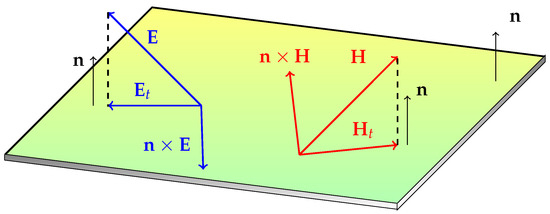
Figure 1. The electric and magnetic fields with their components ${\mathbf{E}}_t,{\mathbf{H}}_t$ tangential to the boundary surface (the unit normal vector is $\mathbf{n}$). The vector $\mathbf{n}\times \mathbf{E}$ has the same magnitude as ${\mathbf{E}}_t$ but is rotated by 90${}^{\circ }$ on the surface; likewise $\mathbf{n}\times \mathbf{H}$ and ${\mathbf{H}}_t$.

If both the normal and tangential components of both the electric and magnetic fields are included, we are led to a rather general class on boundary conditions [8]. In the following, we will however focus on a particular subclass of boundaries; so-called impedance boundaries for which the boundary condition involves only tangential electric and magnetic fields:

$${\mathbf{E}}_{\mathit{t}}={\overline{\overline{\mathsf{Z}}}}_{\mathit{s}}·\left(\mathbf{n}\times {\mathbf{H}}_{\mathit{t}}\right).$$

(1)

This is a dyadic relation on the boundary between the tangential electric and magnetic fields

$${\mathbf{E}}_t=-\mathbf{n}\times (\mathbf{n}\times \mathbf{E})\mathrm{and}{\mathbf{H}}_t=-\mathbf{n}\times (\mathbf{n}\times \mathbf{H}).$$

(2)

The characteristics of the boundary are condensed into the surface impedance dyadic ${\overline{\overline{\mathsf{Z}}}}_s$ in (1). It is worth noting that despite the apparent simplicity of this impedance equation, due to the two-dimensionally dyadic nature of ${\overline{\overline{\mathsf{Z}}}}_{\mathit{s}}$, it spans a very rich domain of boundary conditions.

To classify impedance boundary conditions, take an orthonormal set on real unit vectors $(\mathbf{v},\mathbf{w},\mathbf{n})$ that form a right-handed base. Vectors $\mathbf{v}$ and $\mathbf{w}$ are hence tangential to the boundary. Using these vectors and following ([12] [Sec. 2.9.2]), define the following four elementary two-dimensional dyadics with which all possible impedance dyadics ${\overline{\overline{\mathsf{Z}}}}_s$ can be expanded:

$$\begin{array}{cc}\hfill {\overline{\overline{\mathsf{I}}}}_t& =\mathbf{v}\mathbf{v}+\mathbf{w}\mathbf{w},\hfill \end{array}$$

(3)

$$\begin{array}{cc}\hfill \overline{\overline{\mathsf{J}}}& =\mathbf{n}\times {\overline{\overline{\mathsf{I}}}}_t=\mathbf{w}\mathbf{v}-\mathbf{v}\mathbf{w},\hfill \end{array}$$

(4)

$$\begin{array}{cc}\hfill \overline{\overline{\mathsf{K}}}& =\mathbf{v}\mathbf{v}-\mathbf{w}\mathbf{w},\hfill \end{array}$$

(5)

$$\begin{array}{cc}\hfill \overline{\overline{\mathsf{L}}}& =\mathbf{v}\mathbf{w}+\mathbf{w}\mathbf{v}.\hfill \end{array}$$

(6)

Here ${\overline{\overline{\mathsf{I}}}}_t$ is a two-dimensionally isotropic unit dyadic with which PEC, PMC, and scalar impedance surfaces are characterized. The dyadic $\overline{\overline{\mathsf{J}}}$ is a rotation dyadic (operating on a tangential vector, it changes the vector direction by ${90}^{\circ }$ in the plane). This dyadic is also isotropic as can be seen from the form $\mathbf{n}\times {\overline{\overline{\mathsf{I}}}}_t$ which gives preference neither to $\mathbf{v}$ nor $\mathbf{w}$. The dyadic $\overline{\overline{\mathsf{J}}}$ is needed for the surface impedance of the PEMC boundary.

The two remaining dyadics $\overline{\overline{\mathsf{K}}}$ and $\overline{\overline{\mathsf{L}}}$ are anisotropic in the plane of the surface, having eigenvectors $(\mathbf{v},\mathbf{w})$ and $(\mathbf{v}+\mathbf{w},\mathbf{v}-\mathbf{w})$, respectively. In the following analysis, it is the anisotropy of the surface impedance that is exploited to generate particular properties for the electromagnetic reflection from the boundary.

Using matrix formulation within the $(\mathbf{v},\mathbf{w})$ basis, these dyadics appear as the following $2\times 2$ matrices:

$$I_t=\left(\begin{array}{cc}+1& 0\\ 0& +1\end{array}\right),J=\left(\begin{array}{cc}0& -1\\ +1& 0\end{array}\right),K=\left(\begin{array}{cc}+1& 0\\ 0& -1\end{array}\right),L=\left(\begin{array}{cc}0& +1\\ +1& 0\end{array}\right).$$

(7)

3. Co-Circular Polarization Boundary

From the mathematical nature of the surface impedance dyadic ${\overline{\overline{\mathsf{Z}}}}_s$, several of the characteristics of the boundary are straightforwardly visible. For example, a boundary is lossless (an electromagnetic wave interacting with the boundary neither loses nor gains energy) as long as the impedance dyadic is anti-Hermitian. This means, mathematically, that the ${\overline{\overline{\mathsf{Z}}}}_s$ dyadic in (1) satisfies

$${\overline{\overline{\mathsf{Z}}}}_s^T=-{\overline{\overline{\mathsf{Z}}}}_s^{*},$$

(8)

in other words, its transpose (the superscript T) is the negative of its complex conjugate (the superscript *) ([12] [Sec. 3.6.1]). From this, it follows that for a lossless boundary with symmetric impedance dyadic, ${\overline{\overline{\mathsf{Z}}}}_s$ must be purely imaginary, while the antisymmetric part of the dyadic (like in the case of PEMC) has to be real.

In the following, boundaries with lossless and symmetric impedances will be treated. Hence the impedance dyadic ${\overline{\overline{\mathsf{Z}}}}_s$ is purely imaginary. (Obviously, PEC and PMC boundaries are also lossless, although their impedances are not generally associated with imaginary values, but as long as the impedance magnitude (or its inverse) vanishes, it does not matter whether it is real or imaginary). The time-harmonic notation of the analysis is $exp\left(\mathrm{j}\omega t\right)$.

In order to introduce the main topic of the article, co-circular polarization reflector (CCPR), it is useful to start with two fundamental lossless boundaries: soft-and-hard surface (SHS) and perfectly anisotropic boundary (PAB).

3.1. Soft-and-Hard Surface (SHS)

The so-called soft-and-hard surface is a boundary at which in one tangential direction (along vector $\mathbf{u}$), both the electric and magnetic fields have to vanish:

$$\mathbf{u}·\mathbf{E}=0,\mathbf{u}·\mathbf{H}=0(\mathbf{n}·\mathbf{u}=0).$$

(9)

Such a surface can be fabricated by a corrugated metal structure [13]. While the conductor short-circuits the electric field, the corrugations, as quarter-wavelength waveguides, act as magnetic conductors, thus also forcing the magnetic field along the direction of the corrugations to vanish. Such surfaces have been shown to be useful, for example in the design of horn antennas with symmetrical radiation patterns and low cross-polarization [14,15,16].

The SHS conditions (9) can be written in terms of the impedance boundary condition (1) with the following impedance dyadic:

$${\overline{\overline{\mathsf{Z}}}}_{s,\mathrm{SHS}}=\mathrm{j}{\eta }_0\underset{\delta \to 0}{lim}\left(\delta \mathbf{u}\mathbf{u}+\frac{1}{\delta }(\mathbf{n}\times \mathbf{u})(\mathbf{n}\times \mathbf{u})\right),$$

(10)

where the free-space impedance ${\eta }_0=\sqrt{{\mu }_0/{\epsilon }_0}$ gives units for the surface impedance. [in fact, the coefficient $\mathrm{j}$ in (10) is irrelevant in the limit when $\delta$ vanishes; its meaning there is only to emphasize the lossless character of SHS (cf. Equation (8))].

3.2. Perfectly Anisotropic Boundary (PAB)

The definition of a perfectly anisotropic boundary [17] is that its impedance dyadic is both symmetric and trace-free ([8] [Sec. 3.7]):

$${\overline{\overline{\mathsf{Z}}}}_{s,\mathrm{PAB}}={\overline{\overline{\mathsf{Z}}}}_{s,\mathrm{PAB}}^T,\mathrm{tr}{\overline{\overline{\mathsf{Z}}}}_{s,\mathrm{PAB}}=0,$$

(11)

from which it follows that the dyadic cannot have components ${\overline{\overline{\mathsf{I}}}}_t$ (Equation (3)) or $\overline{\overline{\mathsf{J}}}$ (Equation (4)). It can be expanded as

$${\overline{\overline{\mathsf{Z}}}}_{s,\mathrm{PAB}}=Z_K\overline{\overline{\mathsf{K}}}+Z_L\overline{\overline{\mathsf{L}}}.$$

(12)

For the case that both $Z_K$ and $Z_L$ are non-zero, the eigenvectors of this dyadic are neither $(\mathbf{v},\mathbf{w})$ nor $(\mathbf{v}+\mathbf{w},\mathbf{v}-\mathbf{w})$ like they are for $\overline{\overline{\mathsf{K}}}$ and $\overline{\overline{\mathsf{L}}}$. The (unnormalized, mutually perpendicular) eigenvectors of ${\overline{\overline{\mathsf{Z}}}}_{s,\mathrm{PAB}}$ in (12) are

$${\mathbf{p}}_1=\left(Z_K+\sqrt{Z_K^2+Z_L^2}\right)\mathbf{v}+Z_L\mathbf{w},{\mathbf{p}}_2=\left(Z_K-\sqrt{Z_K^2+Z_L^2}\right)\mathbf{v}+Z_L\mathbf{w},$$

(13)

with eigenvalues

$${\lambda }_1=\sqrt{Z_K^2+Z_L^2},{\lambda }_2=-\sqrt{Z_K^2+Z_L^2}.$$

(14)

Hence, by rotating the $(\mathbf{v},\mathbf{w})$ axes in the plane of the surface, the dyadic ${\overline{\overline{\mathsf{Z}}}}_{s,\mathrm{PAB}}$ can be written as a multiple of a dyadic ${\overline{\overline{\mathsf{K}}}}^{\prime }={\mathbf{v}}^{\prime }{\mathbf{v}}^{\prime }-{\mathbf{w}}^{\prime }{\mathbf{w}}^{\prime }$. And another rotation brings it into a multiple of an ${\overline{\overline{\mathsf{L}}}}^{\prime }={\mathbf{v}}^{\prime }{\mathbf{w}}^{\prime }+{\mathbf{w}}^{\prime }{\mathbf{v}}^{\prime }$ dyadic, where ${\mathbf{v}}^{\prime }$ and ${\mathbf{w}}^{\prime }$ are unit vectors along ${\mathbf{p}}_1$ and ${\mathbf{p}}_2$, respectively. This means that to describe a PAB boundary condition, it is sufficient to use only one of the anisotropic dyadic types, either $\overline{\overline{\mathsf{K}}}$ or $\overline{\overline{\mathsf{L}}}$.

The PAB surface has been shown to serve as an effective polarization transformer ([8] [Sec. 3.7]). A linearly polarized incident field becomes elliptically polarized in reflection. The ellipticity and handedness of the reflected wave depend on the angle that the incident electric field vector makes with the eigendirections of the PAB dyadic. Thus, rotating a PAB plate, the polarization state of the reflected wave can be controlled in a continuous manner.

3.3. Generalization into Co-Circular Polarization Boundary (CCPR)

It turns out that the two fundamental boundaries treated above (SHS and PAB) can be elegantly taken as special cases of a more general impedance boundary condition, the perfect co-polarization reflector, presented in [5] with its metamaterial realization. Let us approach the properties of this CCPR boundary from the impedance dyadic point of view.

The CCPR surface impedance dyadic is the following:

$${\overline{\overline{\mathsf{Z}}}}_{s,\mathrm{C}CPR}=\mathrm{j}{\eta }_0\left(-sinh\left(u\right){\overline{\overline{\mathsf{I}}}}_t+cosh\left(u\right)\overline{\overline{\mathsf{L}}}\right)$$

(15)

which in the matrix form, using the base $(\mathbf{v},\mathbf{w})$, reads

$$\mathrm{j}{\eta }_0\left(\begin{array}{cc}-sinh\left(u\right)& cosh\left(u\right)\\ cosh\left(u\right)& -sinh\left(u\right)\end{array}\right).$$

(16)

The impedance dyadic is a function of a dimensionless parameter u. This parameter is real-valued, in order to secure the lossless character of the CCPR boundary (which is the case when a symmetric impedance dyadic is purely imaginary, cf. Equation (8)).

The symmetry of the dyadic means also that the boundary is reciprocal, in contrast to a non-reciprocal PEMC boundary. Furthermore, while PEMC is isotropic, the CCPR boundary is anisotropic due to the $\overline{\overline{\mathsf{L}}}$ component in (15). However, CCPR is not perfectly anisotropic. This is because its trace does not vanish for non-zero u.

The eigenvectors of ${\overline{\overline{\mathsf{Z}}}}_{s,\mathrm{C}CPR}$ can be easily seen to be $\mathbf{v}$ ± w, with corresponding eigenvalues $\pm \mathrm{j}{\eta }_0\exp (\mp \mathrm{u})$.

The dimensionless parameter u provides variation in the character of the CCPR surface. With the choice $u=0$, the diagonal part of ${\overline{\overline{\mathsf{Z}}}}_{s,\mathrm{C}CPR}$ vanishes, and the impedance becomes $\mathrm{j}{\eta }_0\overline{\overline{\mathsf{L}}}$. This returns us the Perfect anisotropic boundary of Section 3.2.

On the other hand, if $u^{-1}=0$, all the components of the dyadic grow to infinity, but CCPR can be shown to become equal to the soft-and-hard surface (SHS) of Section 3.1. For this case, the direction of the corrugations that short-circuit both the electric and magnetic fields, is $\mathbf{v}+\mathbf{w}$. Note that despite the extreme-looking anisotropic surface impedance (10), SHS is not perfectly anisotropic because, again, the trace of the dyadic is non-zero.

As a side note, the single-parameter CCPR impedance in (15) can be generalized into a two-parameter surface impedance:

$${\overline{\overline{\mathsf{Z}}}}_{s,\mathrm{g}eneral}=\mathrm{j}\eta \left(-sinh\left(u\right){\overline{\overline{\mathsf{I}}}}_t+cosh\left(u\right)\overline{\overline{\mathsf{L}}}\right)$$

(17)

where the scalar impedance $\eta$ needs no longer be the natural constant ${\eta }_0$. To include this $\eta$ parameter in the boundary condition is logical in the sense that it would generalize the full PAB boundary. PAB itself is a one-parameter boundary with the impedance magnitude multiplying its anisotropic dyadic $\overline{\overline{\mathsf{K}}}$ or $\overline{\overline{\mathsf{L}}}$. However, it turns out that the co-circular reflection character does not hold for (17) unless $\eta ={\eta }_0$. Hence in the following, only the one-parameter CCPR (15) is treated.

4. Reflection Dyadic

To analyze the response of the CCPR surface to electromagnetic excitation, consider a plane wave that hits the surface with angle $\theta$ as in Figure 2. The incident wave has a wave vector which can be split into the tangential and normal components: ${\mathbf{k}}^i={\mathbf{k}}_t-k_n\mathbf{n}$, and the reflected wave vector reads accordingly ${\mathbf{k}}^r={\mathbf{k}}_t+k_n\mathbf{n}$. The magnitude of both vectors is the wave number in free space: ${\mathbf{k}}^i·{\mathbf{k}}^i={\mathbf{k}}^r·{\mathbf{k}}^r={\mathbf{k}}_t·{\mathbf{k}}_t+k_n^2=k_0^2$.

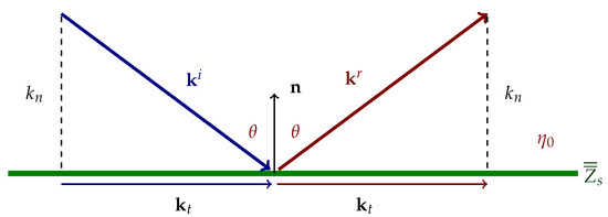
Figure 2. Geometry of the wave reflection. The unit normal $\mathbf{n}$ points into the domain where the fields exist.

Given the polarization state and angle of the incident wave, the reflected wave is determined by the boundary conditions through the reflection dyadic. Define the transversal reflection dyadic ${\overline{\overline{\mathsf{R}}}}_t$ as the relation between the reflected and incident tangential electric fields at the boundary:

$${\mathbf{E}}_t^r={\overline{\overline{\mathsf{R}}}}_t·{\mathbf{E}}_t^i.$$

(18)

Knowing the surface impedance dyadic ${\overline{\overline{\mathsf{Z}}}}_s$, the transversal reflection dyadic can be computed as follows ([8] [Sec. 3.3]):

$${\overline{\overline{\mathsf{R}}}}_t={\overline{\overline{\mathsf{I}}}}_t+2{\eta }_0{\left({\overline{\overline{\mathsf{Z}}}}_s·\mathbf{n}\times {\overline{\overline{\mathsf{J}}}}_t-{\eta }_0{\overline{\overline{\mathsf{I}}}}_t\right)}^{-1}$$

(19)

where the ${\overline{\overline{\mathsf{J}}}}_t$ dyadic expresses the relation between the tangential electric and magnetic fields $({\mathbf{E}}_t^i={\overline{\overline{\mathsf{J}}}}_t·{\eta }_0{\mathbf{H}}_t^i)$:

$${\overline{\overline{\mathsf{J}}}}_t=\frac{1}{k_n{k}_0}\mathbf{n}\times \left({\mathbf{k}}_t{\mathbf{k}}_t+k_n^2{\overline{\overline{\mathsf{I}}}}_t\right).$$

(20)

From this it easily follows that ${\overline{\overline{\mathsf{J}}}}_t·{\overline{\overline{\mathsf{J}}}}_t=-{\overline{\overline{\mathsf{I}}}}_t$, and hence the tangential magnetic field can analogously be computed from the tangential electric field: ${\eta }_0{\mathbf{H}}_t^i=-{\overline{\overline{\mathsf{J}}}}_t·{\mathbf{E}}_t^i$.

As an example of the use of the reflection dyadic formula, consider a simple isotropic impedance surface where the dyadic is a multiple of the transversal unit dyadic:

$${\overline{\overline{\mathsf{Z}}}}_{s,\mathrm{iso}}=Z{\overline{\overline{\mathsf{I}}}}_t.$$

(21)

Substituting this into (19) leads to the following known reflection eigenvalues ([18] [Sec. 8.4]):

$${\overline{\overline{\mathsf{Z}}}}_{s,\mathrm{iso}}=\frac{Z-{\eta }_{0}cos\theta }{Z+{\eta }_{0}cos\theta }\mathbf{p}\mathbf{p}+\frac{Zcos\theta -{\eta }_0}{Zcos\theta +{\eta }_0}\mathbf{s}\mathbf{s}\left(cos\theta =\frac{k_n}{k_0}\right)$$

(22)

where the unit vectors $\mathbf{p}$ and $\mathbf{s}$ refer to the eigenpolarizations in reflection (: in optics, the “p” refers to parallel polarization (transversal magnetic, TM), and “s” to the perpendicular polarization (“senkrecht”, transversal electric, TE)).

$$\mathbf{p}=\frac{{\mathbf{k}}_t}{|{\mathbf{k}}_t|},\mathbf{s}=\frac{\mathbf{n}\times {\mathbf{k}}_t}{|\mathbf{n}\times {\mathbf{k}}_t|}.$$

(23)

5. Reflection Properties of CCPR

The reflection by an arbitrary incident wave from a CCPR surface can be computed using the reflection dyadic in (19). However, due to the anisotropic nature of the surface, the reflection is dependent not only on the polarization and the incidence angle $\theta$ but also the azimuthal direction of the incidence $\phi$. When the CCPR impedance (15) is substituted in (19), the four components of the resulting dyadic (co- and cross-polarized reflection coefficients for the p and s polarizations) are rather lengthy and they depend on three parameters: the angles $\theta$ and $\phi$ and the scalar CCPR parameter u.

5.1. Reflection for Normal Incidence

Fortunately, the characteristics of the CCPR surface can be well appreciated from the special case of normal incidence reflection, in other words ${\mathbf{k}}_t=0$ and $k_n=k_0$, as shown in Figure 3.

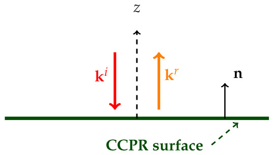
Figure 3. Reflection geometry for a normally incident wave on a CCPR surface.

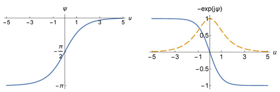
After certain algebraic steps, it is possible to express the reflection dyadic ${\overline{\overline{\mathsf{R}}}}_t$ for this case $\theta =0$ in the form

$${\overline{\overline{\mathsf{R}}}}_{t,\mathrm{CCPR}}=\frac{\mathrm{j}-sinhu}{coshu}\overline{\overline{\mathsf{L}}}=-{\mathrm{e}}^{\mathrm{j}\psi }\overline{\overline{\mathsf{L}}}$$

(24)

where the angle $\psi$ is determined by u in the following manner

$$\psi =\left\{\begin{array}{cc}\mathrm{arccot}(-sinhu)\hfill & u\ge 0,\hfill \\ \mathrm{arccot}(-sinhu)-\pi \hfill & u\le 0.\hfill \end{array}\right.$$

(25)

Since $\psi$ is real-valued, the reflection dyadic amplitude $-exp\left(\mathrm{j}\psi \right)$ is of unit magnitude, as illustrated in Figure 4.

Figure 4. The angle $\psi$ (25) as function of u (left) and the reflection dyadic components in (24): solid blue line—real part; dashed orange—imaginary part (right).

5.2. Behavior of Polarization in Reflection

The reflection dyadic (24) has an extremely condensed expression. Its properties dictate the way the polarization of the incident wave is transformed.

5.2.1. Linear Polarization

Consider a linearly polarized normally wave incident on the CCPR boundary:

$${\mathbf{E}}^i=\left(\mathbf{v}cos\alpha +\mathbf{w}sin\alpha \right)E^i.$$

(26)

The reflected electric field reads (using the reflection dyadic (24))

$${\mathbf{E}}^r={\overline{\overline{\mathsf{R}}}}_{t,\mathrm{CCPR}}·{\mathbf{E}}^i=-{\mathrm{e}}^{\mathrm{j}\psi }\left(\mathbf{v}sin\alpha +\mathbf{w}cos\alpha \right)E^i.$$

(27)

Hence the (linear) polarization of the reflected field is rotated and it experiences a phase shift (but the amplitude remaining unchanged in this lossless reflection). The rotation (Figure 5) depends on the angle $\alpha$ between the incident polarization and the eigenvectors of the CCPR surface. For $\alpha =0$, the reflection is rotated by ${90}^{\circ }$, while for $\alpha ={45}^{\circ }$, the plane of polarization remains.

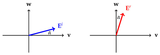
Figure 5. A linearly incident plane wave is rotated in reflection from the CCPR surface. The rotation angle depends on the angle between the plane of polarization of the incident wave and the anisotropy of the surface (with eigenvectors $\mathbf{v}$ and $\mathbf{w}$).

While this polarization plane rotation is independent of the CCPR parameter u, the phase discontinuity $-\exp \left(\mathrm{j}\psi \right)$ is not. As illustrated in Figure 4, it can have values between 0 and $\pi$. For a PAB surface ($u=0$), the phase difference is $\pi /2$. For the SHS boundary, it is either 0 or $\pi$, depending on the orientation of the soft and hard axes diagonally within the ($\mathbf{v},\mathbf{w}$) plane.

5.2.2. Circular Polarization

For a right-handed circularly polarized (RHCP) incident plane wave, the vector reads

$${\mathbf{E}}^i=\left(\frac{\mathbf{v}+\mathrm{j}\mathbf{w}}{\sqrt{2}}\right)E^i\left(\mathrm{RHCP}\right)$$

(28)

(Note that the incident wave propagates in the direction of $-\mathbf{n}$, and the triplet $(\mathbf{v},\mathbf{w},\mathbf{n})$ is right-handed [19]).

The reflected wave becomes

$${\mathbf{E}}^r={\overline{\overline{\mathsf{R}}}}_{t,\mathrm{CCPR}}·{\mathbf{E}}^i=-\mathrm{j}{\mathrm{e}}^{\mathrm{j}\psi }\left(\frac{\mathbf{v}-\mathrm{j}\mathbf{w}}{\sqrt{2}}\right)E^i\left(\mathrm{RHCP}\right)$$

(29)

The reflected wave is also right-handed circularly polarized (because now the triplet $(\mathbf{v},-\mathbf{w},-\mathbf{n})$ is right-handed).

A similar co-polarization phenomenon happens for a left-handed circularly polarized (LHCP) wave incident on the boundary: the reflection is LHCP:

$${\mathbf{E}}^i=\left(\frac{\mathbf{v}-\mathrm{j}\mathbf{w}}{\sqrt{2}}\right)E^i\left(\mathrm{LHCP}\right)\Rightarrow {\mathbf{E}}^r=\mathrm{j}{\mathrm{e}}^{\mathrm{j}\psi }\left(\frac{\mathbf{v}+\mathrm{j}\mathbf{w}}{\sqrt{2}}\right)E^i\left(\mathrm{LHCP}\right)$$

(30)

Hence the label CCPR for this surface is deserved: the handedness of a circular polarization is retained in reflection. This CCPR property does not depend on the parameter u. As evident from (29), u only affects the phase (through $\psi$ in (25)) of the reflected wave. It is worth noting the sign difference between the phases of RHCP and LHCP reflections.

5.2.3. Comparison of Reflection from Various Boundary Conditions

The reflection characteristics of fundamental impedance surfaces (PEC, PMC, PEMC, CCPR (with special caes PAB and SHS)) are summarized in Table 1.

Table 1. Properties of the reflected field polarization for a normally incident fields on various boundaries. The PEMC boundary (with PEMC parameter M) is a generalization of PEC ($M^{-1}=0$) and PMC ($M=0$) boundaries.

	PEC	PMC	PEMC	CCPR
Reflected power	100%	100%	100%	100%
Eigenpolarizations	any	any	RHCP, LHCP	LP ($\mathbf{v}+\mathbf{w},\mathbf{v}-\mathbf{w}$)
Polarization for LP incidence	remains	remains	rotates	rotates
Phase shift for LP	$\pi$	0	0, $\pi$	$\psi +\pi$
Handedness for CP	changes	changes	changes	remains
Phase shift for CP	$\pi$	0	$2\mathrm{arccot}\left(M{\eta }_0\right)-\pi$	$\psi \mp \pi$

5.3. Matched Waves for CCPR Surface

The concept of matched wave was coined in 2017 [20] as plane waves (homogeneous or inhomogeneous) that can exist independently when interacting with a surface. In other words, an incident plane wave does not need a reflected wave to match the boundary conditions as its electrical and magnetic fields already satisfy those. Likewise, a reflected wave which satisfies the boundary conditions, can be called a matched wave.

A way of solving matched incident waves for a given boundary is to search for zeros for reflection dyadic eigenvalues (alternatively, looking for zeros of the inverse of the reflection dyadic to find matched reflected waves).

The condition for a matched wave for a general impedance surface is ([8] [Sec. 3.4])

$$k_0{k}_n\left({\eta }_0^2+{\det }_t{\overline{\overline{\mathsf{Z}}}}_s\right)+{\eta }_0\left({\overline{\overline{\mathsf{Z}}}}_s:{\mathbf{k}}_t{\mathbf{k}}_t+k_n^2\mathrm{tr}{\overline{\overline{\mathsf{Z}}}}_s\right)=0$$

(31)

where tr ${\overline{\overline{\mathsf{Z}}}}_s$ and det${}_t{\overline{\overline{\mathsf{Z}}}}_s$ denote the trace and two-dimensional determinant of the impedance dyadic, respectively (the double-dot product in (31) between dyads or dyadics is defined ([12], Sec. 2.1.1) as $\mathbf{a}\mathbf{b}:\mathbf{c}\mathbf{d}=(\mathbf{a}·\mathbf{c})(\mathbf{b}·\mathbf{d})$). To find matched waves for a CCPR surface, it is helpful to note that since the boundary is lossless, no wave with $k_n\ne 0$ can be matched. Consequently, matched waves have to be lateral (the incidence angle is $\theta =\pi /2$). Therefore we have $k_n=0$ and ${\mathbf{k}}_t={\mathbf{k}}^i$. The dispersion condition for matched waves (31) simplifies into

$${\overline{\overline{\mathsf{Z}}}}_{s,\mathrm{CCPR}}:{\mathbf{k}}^i{\mathbf{k}}^i=0,{\mathbf{k}}^i=\left(\mathbf{v}cos\phi +\mathbf{w}sin\phi \right)k_0,$$

(32)

where $\phi$ is the usual azimuth angle in the polar coordinates (Figure 6).

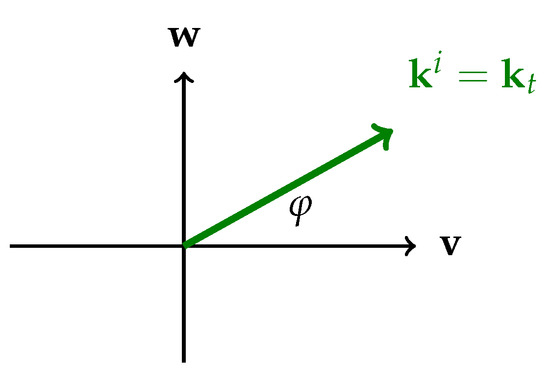
Figure 6. A lateral wave has no normal wave vector component: the wave vector is transversal: ${\mathbf{k}}^i={\mathbf{k}}_t$.

The CCPR impedance dyadic (15) reads

$${\overline{\overline{\mathsf{Z}}}}_{s,\mathrm{CCPR}}=-\mathrm{j}{\eta }_{o}sinhu\left(\mathbf{v}\mathbf{v}+\mathbf{w}\mathbf{w}\right)+\mathrm{j}{\eta }_{o}coshu\left(\mathbf{v}\mathbf{w}+\mathbf{w}\mathbf{v}\right)$$

(33)

which by (32) results in the condition

$$-\left({cos}^2\phi +{sin}^2\phi \right)sinhu+2sin\phi cos\phi coshu=0.$$

(34)

This can be written as

$$sin\left(2\phi \right)=tanhu,$$

(35)

from which we can observe that the lateral wave conditions for two special cases are

$$u=0\left(\mathrm{PAB}\right):\phi =0,\frac{\pi }{2},\pi ,\frac{3\pi }{2},$$

(36)

$$u^{-1}=0\left(\mathrm{SHS}\right):\phi =\frac{\pi }{4},\frac{3\pi }{4},\frac{5\pi }{4},\frac{7\pi }{4}.$$

(37)

For an arbitrary CCPR surface with parameter u, the lateral wave directions $\phi$ are illustrated in Figure 7, as functions of the parameter $\gamma =arctanu$.

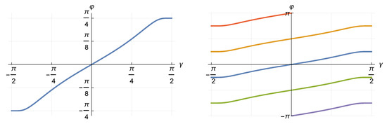
Figure 7. Azimuth angle $\phi$ of the lateral matched wave for a general CCPR surface, as function of the CCPR parameter $\gamma =arctanu$. The multiple azimuth angles are shown on the right-hand side.

6. Conclusions

The focus in the present article has been on electromagnetic wave interaction with planar surfaces that are characterized by a given surface impedance dyadic, a relation between the total tangential electric and magnetic fields on the surface. In particular, the emphasis was on the so-called co-circular polarization reflector (CCPR) surface. This anisotropic and reciprocal surface contains a dimensionless real parameter u. As special cases of the CCPR surface appear (1) the Perfect anisotropic boundary (PAB) for $u=0$, and (2) the Soft-and-hard surface (SHS) for $u^{-1}=0$. For the choice that u is real, the CCPR surface is lossless. Particularly interesting is the behavior of the polarization of waves that interact with CCPR surface: in contrast to PEC, PMC, or PEMC boundaries, the CCPR reflection keeps the handedness of the incident wave in reflection. Linearly and elliptically polarized incident waves are rotated and experience a phase shift that has an intricate connection to the u parameter, thus opening up possibilities to design wide-angle polarization transforming plates and other devices for manipulating properties of waves. Finally, matched waves (wave states that singly satisfy the CCPR impedance boundary condition) were analyzed, and they were shown to be lateral waves (their angle of incidence is ${90}^{\circ }$) but their azimuthal propagation direction in the plane of the CCPR surface again depends on the parameter u.

References

- Kong, J.A. Electromagnetic Wave Theory; EMW Publishing: Cambridge, MA, USA, 2000. [Google Scholar]
- Lindell, I.V.; Sihvola, A.H. Perfect electromagnetic conductor. J. Electromagn. Waves Appl. 2005, 19, 861–869. [Google Scholar] [CrossRef] [Green Version]
- Shahvarpour, A.; Kodera, T.; Parsa, A.; Caloz, C. Arbitrary Electromagnetic Conductor Boundaries Using Faraday Rotation in a Grounded Ferrite Slab. IEEE Trans. Microw. Theory Tech. 2010, 58, 2781–2793. [Google Scholar] [CrossRef]
- El-Maghrabi, H.M.; Attiya, A.; Hashish, E. Design of a Perfect Electromagnetic Conductor (PEMC) Boundary by Using Periodic Patches. Prog. Electromagn. Res. M 2011, 16, 159–169. [Google Scholar] [CrossRef] [Green Version]
- Liu, F.; Xiao, S.; Sihvola, A.; Li, J. Perfect Co-Circular Polarization Reflector: A Class of Reciprocal Perfect Conductors with Total Co-Circular Polarization Reflection. IEEE Trans. Antennas Propag. 2014, 62, 6274–6281. [Google Scholar] [CrossRef]
- Achouri, K.; Caloz, C. Design, concepts, and applications of electromagnetic metasurfaces. Nanophotonics 2018, 7, 1095–1116. [Google Scholar] [CrossRef] [Green Version]
- Liu, Y.; Xu, J.; Xiao, S.; Chen, X.; Li, J. Metasurface Approach to External Cloak and Designer Cavities. ACS Photonics 2018, 5, 1749–1754. [Google Scholar] [CrossRef]
- Lindell, I.V.; Sihvola, A. Boundary Conditions in Electromagnetics; IEEE Press, Wiley: Hoboken, NJ, USA, 2020. [Google Scholar]
- Kildishev, A.V.; Boltasseva, A.; Shalaev, V.M. Planar Photonics with Metasurfaces. Science 2013, 339, 1232009. [Google Scholar] [CrossRef] [PubMed] [Green Version]
- Yu, N.; Capasso, F. Flat Optics with Designer Metasurfaces. Nature Mater. 2014, 13, 139–150. [Google Scholar] [CrossRef] [PubMed]
- Lavigne, G.; Caloz, C. Magnetless reflective gyrotropic spatial isolator metasurface. New J. Phys. 2021, 23, 075006. [Google Scholar] [CrossRef]
- Lindell, I.V. Methods for Electromagnetic Field Analysis; Oxford University Press: Oxford, UK, 1992. [Google Scholar]
- Rotman, W. A Study of Single-Surface Corrugated Guides. Proc. IRE 1951, 39, 952–959. [Google Scholar] [CrossRef]
- Rumsey, V.H. Horn antennas with uniform power patterns around their axes. IEEE Trans. Antennas Propag. 1966, 14, 656–658. [Google Scholar] [CrossRef]
- Kildal, P.S. Definition of artificially soft and hard surfaces for electromagnetic waves. Electron. Lett. 1988, 24, 168–170. [Google Scholar] [CrossRef]
- Kildal, P.S. Artificially soft and hard surfaces in electromagnetics. IEEE Trans. Antennas Propag. 1990, 38, 1537–1544. [Google Scholar] [CrossRef]
- Lindell, I.; Sihvola, A.; Hänninen, I. Perfectly anisotropic impedance boundary. IET Microwaves Antennas Propag. 2007, 1, 561–566. [Google Scholar] [CrossRef] [Green Version]
- Schelkunoff, S.A. Electromagnetic Waves; D. Van Nostrand Company. Inc.: New York, NY, USA, 1943. [Google Scholar]
- IEEE Std 145-198; IEEE Standard Definitions of Terms for Antennas. IEEE: Piscataway, NJ, USA, 1983.
- Lindell, I.V.; Sihvola, A. Generalized Soft-and-Hard/DB Boundary. IEEE Trans. Antennas Propag. 2017, 65, 226–233. [Google Scholar] [CrossRef] [Green Version]
Publisher’s Note: MDPI stays neutral with regard to jurisdictional claims in published maps and institutional affiliations. |
© 2022 by the author. Licensee MDPI, Basel, Switzerland. This article is an open access article distributed under the terms and conditions of the Creative Commons Attribution (CC BY) license (https://creativecommons.org/licenses/by/4.0/).