The Domatic Partition Problem in Separable Graphs

Abstract

The domatic partition problem consists of partitioning a given graph into a maximum number of disjoint dominating sets. This problem is related with the domatic number problem, which consists of quantifying this maximum number of disjoint dominating sets. Both problems were proved to be NP-complete. In this paper, we present a decomposition algorithm for finding a domatic partition on separable graphs, that is, on graphs with blocks, and as a consequence, its domatic number, highly reducing the computational complexity. Computational results illustrate the benefits of the block decomposition algorithm.

1. Introduction

A set of vertices D is a dominating set for a graph $G=(V,E)$ if every vertex in $V\backslash D$ is adjacent to a vertex in D. Several problems related to the concept of dominance have been widely studied in graph theory literature. One of them is the minimum dominating set problem, which consists of obtaining a dominating set of smallest size; it is an NP-hard graph optimisation problem. Another is the problem of obtaining the domatic number $d\left(G\right)$, or domatic number problem, which consists of determining the maximum number of pairwise disjoint dominating sets in which a graph G can be partitioned. If the interest is not only the domatic number but also the elements of the partition, the $d\left(G\right)$ disjoint dominating sets, then the problem is the domatic partition problem (DP).

Domatic number and domatic partition problems are classical optimisation problems which were introduced in the Ref. [1]. Both are NP-complete, even for circular-arc graphs (see the Ref. [2]), but both can be solved in linear time for interval and strongly chordal graphs (see the Ref. [3,4]). Domatic partition/number problems have different applications on the strategic location of facilities or resources in a network. Let us suppose that customers in a network would benefit from the installation of different types of facilities and that the nodes of the network cannot accommodate the installation of more than one type of facility. Let us also suppose that the resources provided by the facilities can only be accessed from neighbouring nodes or from itself. Then, the domatic number is the answer to the question of how many types of essential facilities (e.g., hospitals, universities, computer servers, antennas) can be located in this network, while the domatic partition states where to locate these facilities. Other application fields are related with strategy problems arising from business and military operations.

Currently, there are some known exact algorithms for the domatic number. The Ref. [5] provided an algorithm based on the measure and conquer technique in $\mathcal{O}(2.{8718}^n)$ time and exponential space. At the same time, the Ref. [6] proposed an algorithm based on the principle of inclusion–exclusion in $2^n{n}^{\mathcal{O}\left(1\right)}$ time and exponential space that also runs in $\mathcal{O}(2.{8718}^n)$ time if only polynomial space is used. Finally, the Ref. [7] introduced an algorithm that combines both the measure and conquer and the inclusion–exclusion techniques for calculating the domatic number in $\mathcal{O}(2.{7139}^n)$ time and polynomial space. This algorithm is based on another algorithm for counting the dominating sets in $\mathcal{O}(1.{5673}^n)$ time formulated in the same paper. Thus, given that the domatic number can be calculated from the number of dominating sets of a graph, an improvement in the algorithm used to calculate it automatically implies improving the computational complexity of the domatic number. In this way, in the Ref. [8], a faster algorithm to compute the number of dominating sets of a graph in $\mathcal{O}(1.{5183}^n)$ time was recently introduced. Nevertheless, although the authors comment that this new algorithm can also be used to obtain the domatic number in a faster way, as far as we know, the computational complexity for calculating it using this method has not been evaluated until now.

The majority of the latest exact exponential time algorithms for the domatic number have used both the inclusion–exclusion technique and the measure and conquer technique. The inclusion–exclusion technique was introduced in the Ref. [9]. This technique, usually employed for calculating the size of the intersection of multiple sets or complex probabilities, is based on a simple idea that states it is possible to calculate the size of an intersection of multiple sets by adding the sizes of these sets separately, and then subtracting the sizes of all pairwise intersections from them. The measure and conquer technique was introduced in the Ref. [10]. This is a method to upper bound the total number of subproblems generated mainly by recurrence algorithms, but also by branching algorithms; it is therefore a way of measuring the complexity of these algorithms. However, the use of both techniques in a single algorithm was proposed in the Ref. [11].

Some families of graphs have received special attention when dealing with the domatic number computation; in particular, regular graphs, interval graphs, circular-arc graphs, chordal graphs, block graphs and block-cactus graphs. A graph is said to be regular of degree r if every vertex has the same degree r. It is said to be an interval graph if the nodes represent real line intervals and the edges join vertices whose intervals intersect. Circular-arc graphs are those whose nodes are arcs in a circle and whose edges join vertices whose arcs intersect. A circular-arc graph is a proper circular graph if no arc properly contains another. A chordal graph satisfies that all cycles of four or more vertices have a chord, that is, an edge that connects two vertices of the cycle not being part of the cycle. A block graph is a connected graph such that each maximal connected subgraph without cut-vertices is a complete graph. A block-cactus graph is a graph whose maximal connected subgraphs without cut-vertices are either cycles or complete. There are specific bounds for the domatic number when the network is a regular graph [12]. Additionally, there are linear-time algorithms for solving the domatic number problem in interval graphs [3,13]. While in circular-arc graphs the domatic number problem is NP-complete, it can be solved in $\mathcal{O}(n^{2}log$$n)$ time for proper circular-arc graphs [2]. However, linear time algorithms were developed for strong chordal graphs in the Ref. [4]. Moreover, the domatic number for block-cactus graphs was discussed in the Ref. [14]. As for block graphs, several related problems have been studied for this family of graphs as the power domination number [15], the k-power domination number in the Ref. [16], the k-distance domination problem in the Ref. [17], and even the total domination number, as in the Ref. [18]. However, as far as we know, the domatic number and partition problems have not been analysed for the particular case of graphs that are decomposable into blocks, where blocks are maximal connected subgraphs without cut-vertices. The main purpose of this paper is to propose a specific algorithm for obtaining a domatic partition, and as a consequence, the domatic number, in graphs with blocks. Given that blocks are not required to be complete, our algorithm can be applied to graphs other than block graphs. The new algorithm considerably reduces computation time.

The domatic partition problem has received less attention than the domatic number problem. The exact method for the domatic partition problem is based on linear integer programming. In the Ref. [19], two mixed integer models were discussed for the independent domatic partition problem. Approximating algorithms for the domatic partition can be found in the Ref. [20]. However, to the best of our knowledge, there are not any specific exact algorithms for the domatic partition problem.

This article is aimed to bridge this gap, studying the resolution of the domatic partition problem when the graph contains these special nodes whose removal produces two or more connected components. In other words, the goal of this paper is to develop an exact approach for separable graphs. We propose an exact decomposition algorithm based on the blocks. The algorithm iteratively solves an integer linear problem that we call the allied domatic partition problem. In fact, in order to obtain the solution of the domatic partition problem, we solve the allied domatic partition problem several times. The number of times we solve the allied domatic partition problem depends on the number of blocks of the graph, and also on the accuracy of the initial upper bound we have for the domatic partition problem. The decomposition of the problem considerably reduces the solution’s computational time.

The merits of this paper are threefold. The first merit is showcasing an innovative resolution algorithm for the domatic partition problem focused on decomposing graphs into their blocks. Therefore, this article illustrates the benefit of decomposing as a successful resolution technique. The second merit is introducing a new domination concept, the allied domination, which may help future researchers in the analysis of the domination problem. The third merit is coding the decomposition algorithm and obtaining challenging computational results that show the effectiveness of the algorithm in terms of time reduction.

The following section is about domination problems: the model in the literature for solving the independent domatic partition problem is adapted to model the domatic partiton problem. Moreover, the model for the decomposition algorithm of the following section is introduced. The new model deals with a new concept named allied domination. Section 3 is the main section of this paper: it gives the new algorithm that we propose for obtaining a domatic partition when a graph is separable. In Section 4, the advantages of the new algorithm are analysed by an extensive computational experience. Conclusions and future research are summarised in Section 5.

2. Domination Models

A graph $G=(V,E)$ consists of a vertex set V and an edge set E. The sets $N\left(v\right)=\{u\in V|(v,u)\in E\}$ and $N\left[v\right]=N\left(v\right)\cup \left\{v\right\}$ are the open and closed neighbourhoods of $v\in V$, respectively. The degree of a vertex $v\in V$ is $\left|N\right(v\left)\right|$ and $\delta \left(G\right)$ is the minimum degree of graph G. $S\subseteq V$ is a dominating set of G if all the nodes in V are neighbours of the nodes in $S,$ that is, S is a dominating set if ${\cup }_{u\in S}N\left[u\right]=V.$ It is known that the maximum number of pairwise disjoint dominating sets or domatic number, $d\left(G\right),$ is bounded by the minimum degree of the graph: $d\left(G\right)\le \delta \left(G\right)+1.$ When $d\left(G\right)=\delta \left(G\right)+1,$ the graph G is called domatically full. A component of a graph is a maximal connected subgraph. A vertex whose deletion increases the number of connected components of a graph is called a cut-vertex. Graphs with at least one cut-vertex are also called separable graphs. Finally, a block of a graph is a maximal connected subgraph without cut-vertices. Blocks are not necessarily cliques, that is, blocks can be incomplete. The block-cutpoint graph of G is the bipartite graph with a vertex set $C\cup B$, where C is the set of cut-vertices and B is the set of blocks of G, and node $c\in C$ and $b\in B$ are neighbours if c is a node of block $b.$ It is well-known that the block-cutpoint graph of a connected graph is always a tree. The blocks which are leaves of the block-cutpoint graph are called leaf blocks of $G.$

The domatic partition problem in G is the problem of obtaining a maximal partition of V such that the elements of the partition are pairwise disjoint dominating sets. The problem can be modelled as the following integer linear programming:

$$\begin{array}{cc}\hfill \left(\mathsf{D}\mathsf{P}\right)& \hfill {\displaystyle max\sum _{j=1}^{\delta \left(G\right)+1}{u}_j}\\ \hfill \mathsf{s}.\mathsf{t}.& & \hfill \end{array}$$

(1)

$$\begin{array}{ccc}& {\displaystyle x_u^j+\sum _{v:(u,v)\in E}{x}_v^j\ge u_j}\hfill & \hfill u\in V,j\in \{1,\dots ,\delta (G)+1\}\end{array}$$

(2)

$$\begin{array}{ccc}& \sum _{j=1}^{\delta \left(G\right)+1}{x}_u^j\le 1\hfill & \hfill u\in V\end{array}$$

(3)

$$\begin{array}{ccc}& u_j\in \{0,1\},x_u^j\in \{0,1\}\hfill & \hfill u\in V,j\in \{1,\dots ,\delta (G)+1\},\end{array}$$

(4)

where $u_j$ takes the value of 1 if there is any vertex belonging to the j-th disjoint dominating set, and $x_u^j$ takes the value of one if node u belongs to the j-th dominating set. Constraints (2) express domination, constraints (3) express disjointness between sets, and (4) express binary domains. Finally, the objective function (1) maximises the number of disjoint dominating sets. The index j moves from 1 to $\delta \left(G\right)+1$ because of the inequality $d\left(G\right)\le \delta \left(G\right)+1.$ Once the model is solved on a graph, the objective function value is the domatic number $d\left(G\right)$, whilst the domatic partition is obtained from the variables $x_u^j$ by setting $S_j=\{u\in V:x_u^j=1\}.$ The domatic partition $\mathcal{P}$ is the set of sets $S_j$ that are not empty, that is, $\mathcal{P}=\{S_j:S_j\ne \varnothing ,j\in \{1,\dots ,\delta \left(G\right)+1\}\}$.

Allied Domination

Apart from the well-known dominating sets, in this work we introduce a new concept related to domination that we call allied domination. Suppose that V is split into two disjoint subsets, $V=V_o\cup V_a.$ We say that a subset $D\subseteq V$ is an allied dominating set if every vertex $v\in V_o$ is either in D or adjacent to a vertex in D. The subset $V_o$ is called a subset of own vertices and the subset $V_a$ is called a subset of allied vertices. Note that the difference between the concept of domination and the concept of allied domination is that the domination of allied vertices is not compulsory, although they can contribute to the domination of neighbour vertices. Colloquially, allied nodes can help to dominate, but they must not be dominated. Keeping allied domination in mind, we define the problems of allied domatic partition and allied domatic number as follows. An  allied domatic partition of a graph $G=(V_o\cup V_a,E)$ is a maximum-sized partition of G such that each vertex is in an allied dominating set. The allied domatic number is the size of this partition. The problem of obtaining an allied domatic partition can be modelled as the following integer linear programming problem.

$$\begin{array}{cc}\hfill \left(\mathsf{A}\mathsf{D}\mathsf{P}\right)& {\displaystyle max\sum _{j=1}^{\delta \left(G\right)+1}{u}_j}\hfill \\ \hfill \mathbf{s}.\mathbf{t}.& & \hfill \\ & {\displaystyle x_u^j+\sum _{v:(u,v)\in E}{x}_v^j\ge u_j}\hfill & \hfill u\in V_o,j\in \{1,\dots ,\delta \left(G\right)+1\}\\ & \left(3\right),\left(4\right).\hfill \end{array}$$

(5)

Constraints (5) express domination of vertices $v\in V_o$. The optimal value is the allied domatic number, and the allied domatic partition is obtained from variables $x_u^j$.

When the domination by an allied node $v_a\in V_a$ entails a cost $w_{v_a}$ and the number of disjoint allied dominating sets is fixed to $k,$ the domination problem is the minimum cost allied k-domination partition problem.

$$\begin{array}{cc}\hfill (\mathsf{M}\mathsf{C}-\mathsf{A}\mathsf{k}\mathsf{D}\mathsf{P})& min\sum _{u\in V_a}\sum _{j=1}^{\delta \left(G\right)+1}{w}_u{x}_u^j\hfill \\ \hfill \mathbf{s}.\mathbf{t}.& & \hfill \end{array}$$

(6)

$$\begin{array}{cccc}& {\displaystyle \sum _{j=1}^{\delta \left(G\right)+1}{u}_j=k}\hfill & & \hfill \\ & \left(3\right),\left(4\right),\left(5\right).\hfill & & \hfill \end{array}$$

(7)

MC-AkDP consists of obtaining k disjoint dominating sets at the minimum cost. If k is not fixed, the minimum-cost allied domatic partition problem could also be considered.

3. Block Decomposition Algorithm

In this section, the block decomposition algorithm we propose is presented. In order to understand it, we shall first explain the procedure with an illustrative example, and we shall then describe the general algorithm. Several similar decomposition mechanisms have been described in the literature for other graph problems, see, for example, Refs. [21,22].

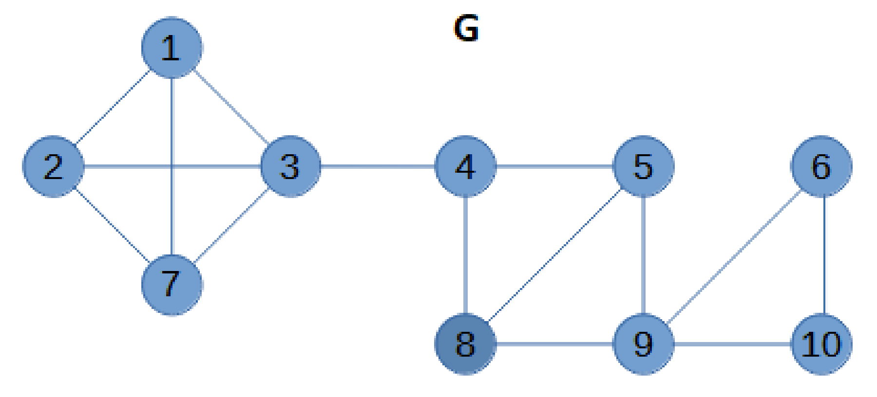
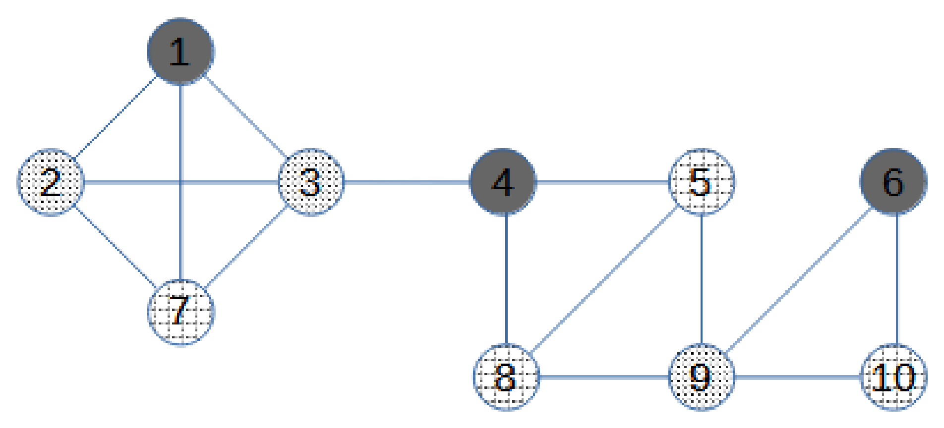
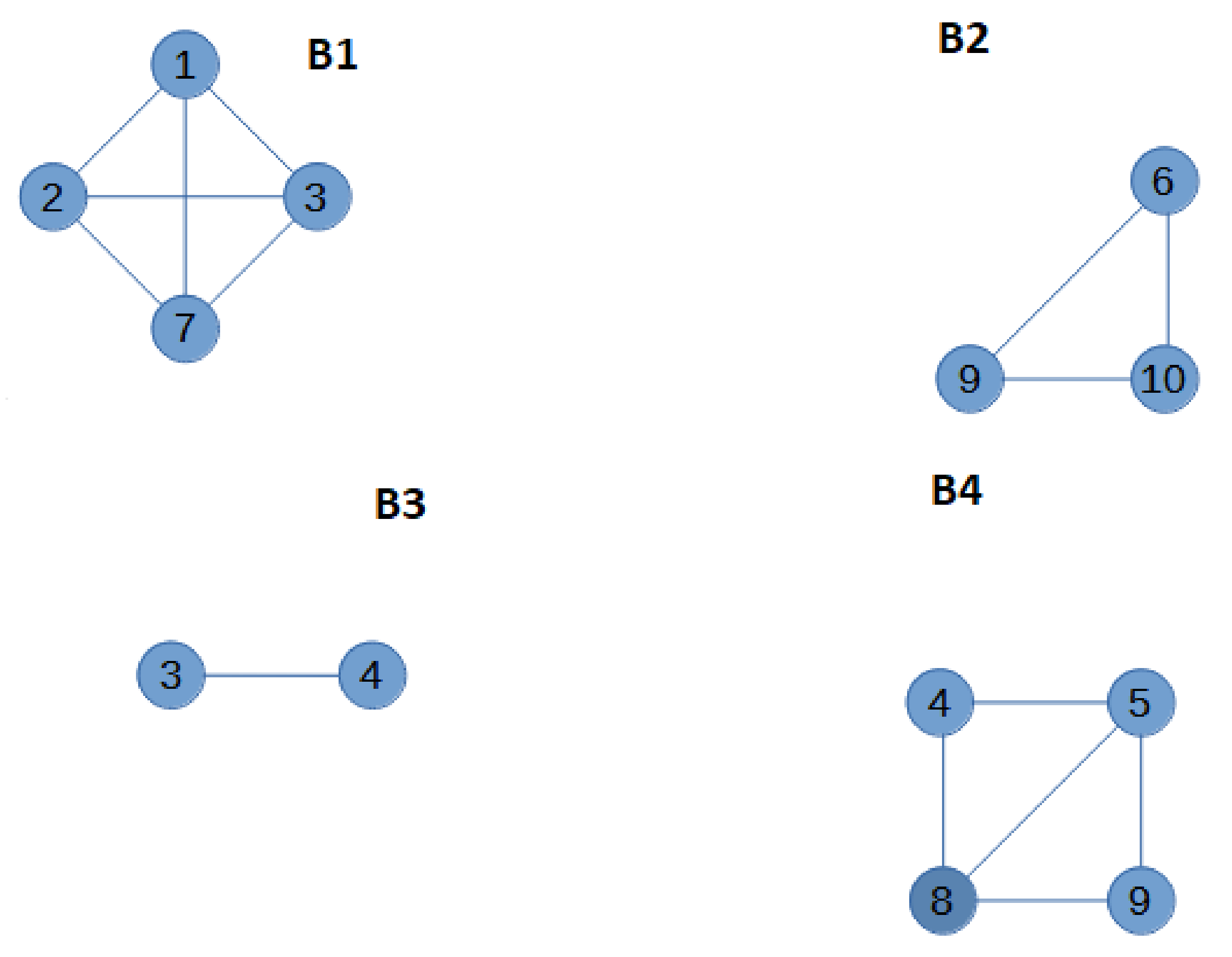
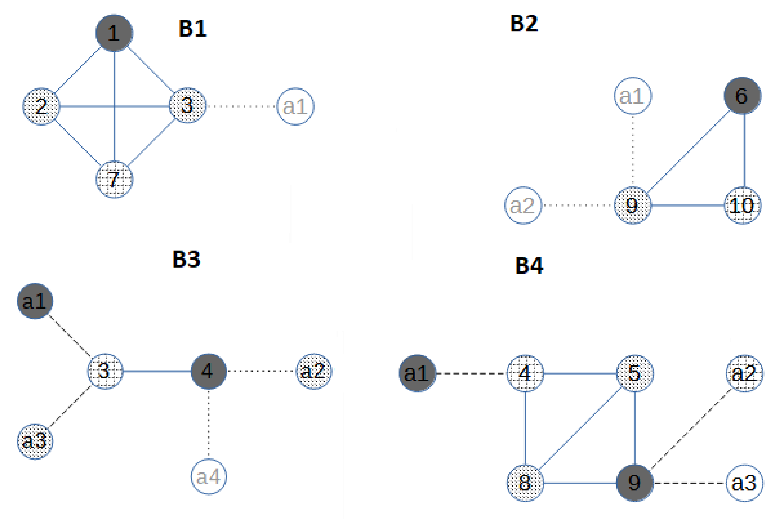
Let us consider the graph in Figure 1. Before starting the iterative process, we update the upper bound ($\kappa$) for the domatic number $d\left(G\right)$ to the value 3: $\delta \left(G\right)=2$ is the minimum degree of G, that is, the degree of vertex 6, and $\delta \left(G\right)+1$ is an upper bound to $d\left(G\right).$ Then, the graph is split into blocks. All the blocks are the four subgraphs in Figure 2. The blocks are sorted from the leaf blocks to the root block. In the example, blocks B1 and B2 are leaf blocks, and both are followed by blocks B3 and B4. Ties in the order can be broken arbitrarily. For the first block $B1$, we build an augmented block $\overline{B1}$ by adding allied nodes to the cut-vertices of the block, and to each cut-vertex, an allied node for each neighbour of the cut-vertex that is not in the block is added. B1 has only one cut-vertex, node 3. The only neighbour of 3 that is not in B1 is node 4, so only one allied vertex is added to $B1$. The  augmented first block $\overline{B1}$ is in Figure 3. The weight $w_{a_1}=1$ is assigned to the allied vertex in $\overline{B1}$. Then, we solve MC-AkDP for $\overline{B1}$ with $\kappa =3$ (3 is an upper bound for $d\left(G\right)$). Note that the weight $w_{a_1}=1$ implies that if possible, the allied dominating set in $\overline{B1}$ does not make use of node $a_1$, and thus the domatic partitions in adjacent blocks do not need to be coherent with their position in the partition. An optimal solution for MC-AkDP($\overline{B1},w,\kappa )$ is the one in Figure 2: there are three dominating sets in $\overline{B1}$, which are described by the three grey colours. Then, a similar procedure is carried on with the following block B2. B2 has one cut-vertex, node 9, and the number of neighbours of 9 that are not in B2 is two, so the augmented block $\overline{B2}$ has two allied nodes with unitary weight, $w_{a1}=w_{a2}=1.$ The optimal value of MC-AkDP($\overline{B2},w,\kappa )$ is zero because there are three dominating sets in $\overline{B2}$, the three grey colours in in Figure 2. Block B3 has two cut-vertices, nodes 3 and 4. From now on, the number of allied vertices connected to a cut-vertex is not always the number of neighbours outside the block. Given a cut-vertex, if the problem MC-AkDP has been solved for other blocks connected to the same cut-vertex, the number of allied vertices connected to it must be $\kappa -1$ minus the optimal solution of the previous MC-AkDP problem. For node 3, the number of allied vertices must be $\kappa -1$ minus the optimal value of MC-AkDP($\overline{B1},w,\kappa ),$ that is 2 (3-1-0). For node 4, no other problem associated to an augmented incident block has been solved, so it has as many allied vertices as neighbours outside the block, that is, two allied vertices. Analogously, the weight is not directly one anymore; if some incident block to the cut-vertex was previously solved, then the weight is zero. Thus, in $\overline{B3}$, $w_{a1}=w_{a3}=0$ and $w_{a2}=w_{a4}=1$. In Figure 3, Weight One is indicated by light dashed grey lines, and Weight Zero by dark dashed grey lines. The optimal value of MC-AkDP($\overline{B3},w,\kappa )$ is one because the allied node a2 is used for having three dominating sets. The last block B4 has two cut-vertices and both were the cut-vertex in previously solved MC-AkDP problems. Thus, the number of allied vertices connected to node 4 is $\kappa -1$ minus the optimal value of MC-AkDP($\overline{B3},w,\kappa )$ and the number of allied vertices connected to node 9 is $\kappa -1$ minus the optimal value of MC-AkDP($\overline{B2},w,\kappa ):$ one allied vertex to node 4 and two allied vertices to node 9. The weight for the three allied vertices is zero and the optimal solution for the MC-AkDP($\overline{B4},w,\kappa )$ is the one in Figure 3. Finally, if  some of the MC-AkDP problems would not have had a solution, that is, it would have been impossible to have a domatic partition of size $\kappa$, we would have updated $\kappa$ to $\kappa -1$ and started again.

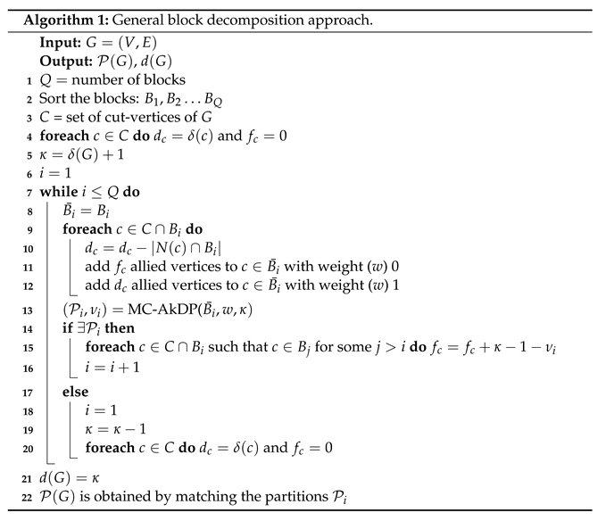
The general decomposition approach that is described in Algorithm 1 keeps the same spirit as the procedure described for the small example. It starts by sorting the blocks and initialising the number of allied vertices for any cut-vertex. The iterative pool of actions goes from line 7 to line 20. For the cut-vertex that connects the block to the tree of blocks, $\delta \left(r\right)-|N\left(r\right)\cap B_{i\left(r\right)}|$ allied vertices are added, while for the other cut-vertices $\kappa -1-{\nu }_{B_i}$, allied vertices are added. Weights are used to minimise the number of allied nodes in the domination of r. Unweighted nodes were already used in a previous iteration, and we can make use of it freely. In line 13, ${\nu }_i$ is the optimal value of the MC-AkDP problem, representing the minimum number of weighted allied nodes needed for the domination, and ${\mathcal{P}}_i$ is the partition of $B_i$ obtained from variables $x_u^j$ (it is $\mathcal{P}=\{S_j:S_j\ne \varnothing ,j\in \{1,\dots ,\delta \left(G\right)+1\}\}$ where $S_j=\{u\in V:x_u^j=1\}$ for all $j\in \{1,\dots ,\delta (G)+1).$ If any optimisation problem MC-AkDP is unfeasible, the $\kappa$ is reduced by one unit. The last line of Algorithm 1 refers to Algorithm 2, which states how to paste all the allied dominating sets in the blocks into one dominating set of the total graph.

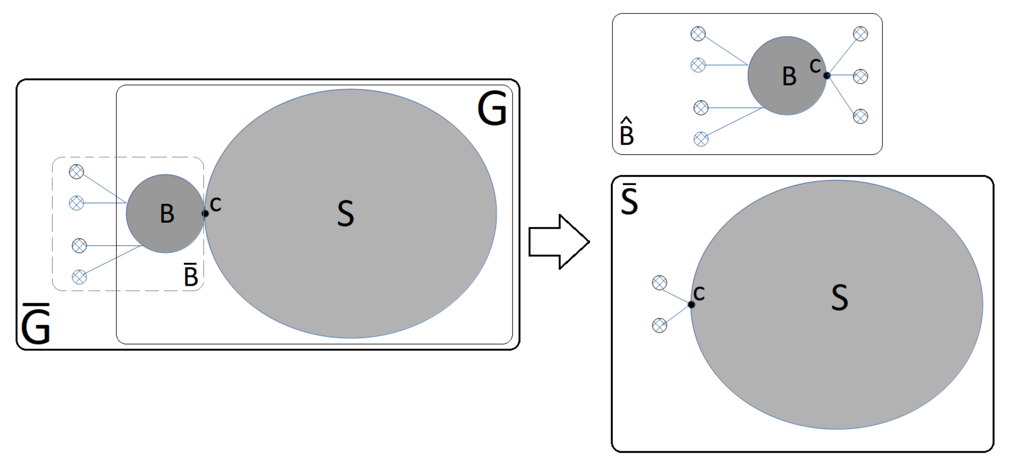
In Propositions 1–8 we will prove that the output of Algorithm 1 is a domatic partition. The main goal is to prove that the MC-AkDP problem of separable graphs can be solved by solving the MC-AkDP problem of one block and the MC-AkDP problem of a related connected subgraph. As we can recursively repeat this operation until the subgraph is non-separable, that is, a block, then the MC-AkDP problem of a separable graph can be solved by solving one MC-AkDP problem for each of its blocks. Figure 4 represents the elements that are used in the propositions. These usually are:

• A separable graph $G=(V,E)$;
• A leaf block $B\in G$;
• A cut-vertex of B named as c;
• A connected subgraph $S\in G$ such that $B\cup S=G$ and $c=B\cap S;$
• An augmented block with allied nodes of weight 0 added to B named as $\overline{B}$; and
• $\overline{G}=\overline{B}\cup S$.

The solved MC-AkDP problems are related to $\overline{G}$ and the added allied nodes of Weight 0 depend on the previously solved blocks. The added allied nodes force to obtain dominating sets which are consistent with the dominating sets of the blocks already solved. We could say, in a colloquial way, that the added allied nodes are the links to the previously solved problems.

Each graph $\overline{G}$ is solved in two steps. First, the graph $\widehat{B}$ obtained by adding $N\left(c\right)\cap S$ allied nodes to $\overline{B}$ (Proposition 1) is processed. Then, the graph $\overline{S}$ is obtained by adding a number of allied nodes to S to be processed. The number of allied nodes added to S depends on the result obtained when $\widehat{B}$ was processed (Proposition 2).

An algorithm for matching the different obtained partitions is described (Algorithm 2) and discussed (Propositions 6 and 7). Finally, Proposition 8 proves that Algorithm 1 returns a domatic partition of G.

Proposition 1.

Let

• $G=(V,E)$ be a separable graph;
• $B\in G$ be a leaf block;
• c be the cut-vertex of $B;$
• $S\in G$ be the connected subgraph such that $B\cup S=G$ and $c=B\cap S;$
• $\overline{B}$ be an augmented block with allied nodes of Qeight 0 added to B;
• $\overline{G}=\overline{B}\cup S$; and
• $\widehat{B}$ be the graph obtained by adding $N\left(c\right)\cap S$ allied nodes to $\overline{B}$.

If MC-AkDP$(\overline{G},w,\kappa )$ has a solution, then MC-AkDP$(\widehat{B},w_{\widehat{B}},\kappa )$ also has a solution.

Proof. 

A feasible solution consists of grouping the nodes of $\widehat{B}$ in the same way that these nodes are grouped in a partition for obtaining $\kappa$ allied dominating sets in $\overline{G},$ which is possible since MC-AkDP$(\overline{G},w,\kappa )$ has a solution and $N\left(c\right)\cap S$ allied nodes were added to $c\in \overline{B}$. Note that these $N\left(c\right)\cap S$ allied nodes do not have to be dominated, but they contribute to the domination of c.    □

Corollary 1.

Proposition 1 is valid independently of the weights imputed to the allied nodes added to $c\in \overline{B}$.

Proof. 

That is because the weights only affect the objective function but neither the number of allied nodes to add nor to the feasible region.    □

Corollary 2.

In Proposition 1, if the allied nodes added to $c\in \overline{B}$ are weighted by 1 and MC-AkDP$(\widehat{B},w_{\widehat{B}},\kappa )={\nu }_{\widehat{B}},$ then $\kappa -1-{\nu }_{\widehat{B}}$ is the maximum number of sets in $\overline{B}$ that can dominate c in a MC-AkDP$(\overline{G},w,\kappa )$ solution.

Proof. 

Since the allied nodes added to $c\in \overline{B}$ when $\widehat{B}$ is built are weighted by 1, then ${\nu }_{\widehat{B}}$ represents the minimum number of allied nodes needed to get $\kappa$ allied dominating sets That implies $\kappa -1-{\nu }_{\widehat{B}}$ is the maximum number of disjoint sets in $\widehat{B}$ that dominate c.    □

Proposition 2.

Let

• $G=(V,E)$ be a separable graph;
• $B\in G$ be a leaf block;
• c be the cut-vertex of $B;$
• $S\in G$ be the connected subgraph such that $B\cup S=G$ and $c=B\cap S;$
• $\overline{B}$ be an augmented block with allied nodes of weight 0 added to B;
• $\overline{G}=\overline{B}\cup S$;
• $\widehat{B}$ be the graph obtained by adding $N\left(c\right)\cap S$ allied nodes with weight 1 to $\overline{B}$;
• ${\nu }_{\widehat{B}}=$ MC-AkDP$(\widehat{B},w_{\widehat{B}},\kappa )$;
• $\overline{S}$ be the graph obtained by adding $\kappa -1-{\nu }_{\widehat{B}}$ allied nodes to S.

If MC-AkDP$(\overline{G},w,\kappa )$ has a solution, then MC-AkDP$(\overline{S},w_{\overline{S}},\kappa )$ also has a solution.

Proof. 

By reductio ad absurdum, if MC-AkDP$(\overline{S},w_{\overline{S}}\kappa )$ does not have a solution, it would either be because not enough allied nodes were added to $c\in S$, or even adding infinite nodes does not guarantee that a solution can be obtained. On the one hand, if it would be possible to add more allied nodes to $c\in S$ to achieve a solution to MC-AkDP$(\overline{S},w_{\overline{S}},\kappa ),$ then MC-AkDP$(\widehat{B},w_{\widehat{B}}\kappa )$ would not have a solution: according to Corollary 1, if the maximum number of disjoint sets in $\overline{B}$ that can dominate c were added, then no more allied nodes can be added. On the other hand, if even adding infinite allied nodes to $c\in S$ would not yield a solution, it would be because MC-AkDP$(\overline{G},w,\kappa )$ does not have a solution. Note that in case the solution exists, it would be enough to group the nodes of S in the same way these are grouped in a MC-AkDP$(\overline{G},w,\kappa )$ and then provide as many allied nodes as needed to get $\kappa$ allied dominating sets.    □

Corollary 3.

Propositions 2 are valid independently of the weights imputed to the allied nodes of $\overline{S}$.

Proof. 

That is because these weights only affect the objective function of MC-AkDP$(\overline{S},w_{\overline{S}},\kappa )$ but not the number of allied nodes to add, nor the feasible region.    □

Proposition 3.

Let

• $G=(V,E)$ be a separable graph;
• $B\in G$ be a leaf block;
• c be the cut-vertex of $B;$
• $S\in G$ be a connected subgraph such that $B\cup S=G$ and $c=B\cap S;$
• $\overline{B}$ be an augmented block with allied nodes of Weight 0 added to B;
• $\overline{G}=\overline{B}\cup S$;
• $\widehat{B}$ be the graph obtained by adding $N\left(c\right)\cap S$ allied nodes with Weight 1 to S; and
• $\overline{S}$ be the graph obtained by adding $\kappa -1-{\nu }_{\widehat{B}}$ allied nodes to S.

If MC-AkDP$(\widehat{B},w_{\widehat{B}},\kappa )$ or MC-AkDP$(\overline{S},w_{\overline{S}},\kappa )$ has no solution, then MC-AkDP$(\overline{G},w,\kappa )$ has no solution.

Proof. 

On the one hand, if MC-AkDP$(\widehat{B},w_{\widehat{B}},\kappa )$ has no solution, that is because MC-AkDP$(\overline{G},w_{\overline{G}}\kappa )$ also has no solution, otherwise a solution of MC-AkDP$(\widehat{B},w_{\widehat{B}},\kappa )$ would be obtained by grouping the nodes of $\widehat{B}$ in the same way these are grouped to obtain $\kappa$ allied dominating sets in $\overline{G}$.

On the other hand, if MC-AkDP$(\overline{S},w_{\overline{S}}\kappa )$ had no solution, it would be because either not enough allied nodes were added to $c\in S$ or because even adding infinite allied nodes to $c\in S$ a solution would not work. In the first case, if it would be possible to add more allied nodes to $c\in S$ to achieve a solution to MC-AkDP$(\overline{S},w_{\overline{S}},\kappa ),$ then MC-AkDP$(\widehat{B},w_{\widehat{B}},\kappa )$ would have no solution—according to Corollary 1, if the maximum number of disjoint sets in $\overline{B}$ that can dominate c were added, then no more allied nodes can be added. In the second case, if by even adding infinite allied nodes to $c\in S$ a solution could not be obtained, that would clearly happen if MC-AkDP$(\overline{G},w,\kappa )$ has no solution.    □

Corollary 4.

Let

• $G=(V,E)$ be a separable graph;
• $B\in G$ be a leaf block;
• c be the cut-vertex of $B;$
• $S\in G$ be the connected subgraph such that $B\cup S=G$ and $c=B\cap S;$
• $\overline{B}$ be an augmented block with allied nodes of Weight 0 added to B;
• $\overline{G}=\overline{B}\cup S$;
• $\widehat{B}$ be the graph obtained by adding $N\left(c\right)\cap S$ allied nodes with weight 1 to $\overline{B}$;
• ${\nu }_{\widehat{B}}=$ MC-AkDP$(\overline{B},w_{\overline{B}},\kappa )$; and
• $\overline{S}$ be the graph obtained by adding $\kappa -1-{\nu }_{\widehat{B}}$ allied nodes to S.

$d_a\left(\overline{G}\right)\ge \kappa$ if and only if both MC-AkDP$(\widehat{B},w_{\widehat{B}},\kappa )$ and MC-AkDP$(\overline{S},w_{\overline{S}},\kappa )$ have a solution.

Proof. 

Remember that $d_a\left(\overline{G}\right)$ is the maximum $\kappa$, such that MC-AkDP$(\overline{G},w_{\overline{G}},\kappa )$ has a solution. On the one hand, Propositions 1 and 2 guarantee that if MC-AkDP$(\widehat{B},w_{\widehat{B}},\kappa )$ and MC-AkDP$(\overline{S},w_{\overline{S}},\kappa )$ have a solution, then MC-AkDP$(\widehat{G},w_{\widehat{G}},\kappa )$ also has a solution. On the other hand, Proposition 3 says that if MC-AkDP$(\widehat{B},w_{\widehat{B}},\kappa )$ or MC-AkDP$(\overline{S},w_S,\kappa )$ have no solution, then G cannot be partitioned into $\kappa$ allied dominating sets. Thus, $\overline{G}$ can be partitioned into $\kappa$ allied dominating sets or what is the same, $d_a\left(G\right)\ge \kappa$, if and only if both MC-AkDP$(\widehat{B},w_{\widehat{B}},\kappa )$ and MC-AkDP$(\overline{S},w_S,\kappa )$ have a solution.    □

Corollary 5.

Let

• $G=(V,E)$ be a separable graph;
• $B\in G$ be a leaf block;
• c be the cut-vertex of $B;$
• $S\in G$ be the connected subgraph such that $B\cup S=G$ and $c=B\cap S;$
• $\overline{B}$ be the augmented block with $N\left(c\right)\cap S$ allied nodes of weight 1 added to B
• ${\nu }_{\overline{B}}=$ MC-AkDP$(\overline{B},w_{\overline{B}},\kappa );$
• $\overline{G}=\overline{B}\cup S$; and
• $\overline{S}$ be the graph obtained by adding $\kappa -1-{\nu }_{\overline{B}}$ allied nodes to S.

$d\left(G\right)\ge \kappa$ if and only if both MC-AkDP$(\overline{B},w_{\overline{B}},\kappa )$ and MC-AkDP$(\overline{S},w_{\overline{S}},\kappa )$ have a solution.

Proof. 

Trivial from Corollary 4. It is the particular case in which $\overline{G}$ has 0 allied nodes.    □

Let $G=(V,E)$ be a separable graph, $B\in G$ a leaf block, and a connected subgraph $S\in G$ such that $B\cup S=G$. Since $d\left(G\right)\ge \kappa$ if and only if both MC-AkDP$(\overline{B},w_{\overline{B}},\kappa )$ and MC-AkDP$(\overline{S},w_{\overline{S}},\kappa )$ have a solution (Corollary 5), then one way to calculate $d\left(G\right)$ consists of setting $\kappa$ by enumerating, for example, by increasing it sequentially from $\kappa =3$ until no solution exists or decreasing it sequentially from $\kappa =\delta \left(G\right)+1$ until both MC-AkDP$(\overline{B},w_{\overline{B}},\kappa )$ and MC-AkDP$(\overline{S},w_{\overline{S}},\kappa )$ have a solution. Other strategies could also be designed in order to save explorations, such as increasing/decreasing procedures with some steps larger than 1.

Proposition 4.

Algorithm 1 returns the domatic number of G.

Proof. 

Algorithm 1 solves $d\left(G\right)$, sequentially decrementing from $\kappa =\delta \left(G\right)+1$. At each iteration it starts trying MC-AkDP$(\overline{B},w_{\overline{B}},\kappa )$ and MC-AkDP$(\overline{S},w_{\overline{S}},\kappa )$, given that if both problems have a solution, that would mean $d\left(G\right)=\kappa$ (Corollary 5). Each MC-AkDP$(\overline{S},w_{\overline{S}},\kappa )$ is recursively solved by decomposing it into leaf blocks according to Proposition 3 until S is also a block. That is equivalent to sorting and solving the blocks from the leaf blocks to the root block as Algorithm 1 does.    □

Proposition 5.

For each block $B_i\in G,$ let ${\mathcal{P}}_i$ be a partition of $B_i$ built by Algorithm 1 but excluding the allied nodes in each subset in ${\mathcal{P}}_i$. Then, a domatic partition of G is obtained by consistently matching the partitions ${\mathcal{P}}_i$.

Proof. 

Each block is solved by adding a number of allied nodes which represent the number of dominating sets that dominate a shared cut-vertex. Its MC-AkDP solution provides $\kappa$ dominating sets. Thus, it is possible to find a domatic partition of G by consistently matching the partitions ${\mathcal{P}}_i$. Note that if the indexes j of the allied nodes were fixed to 1 in variables $x_u^j,$ then the matching would not be necessary.    □

The algorithm that we propose for matching the partitions ${\mathcal{P}}_i$ is Algorithm 2. It starts with partition ${\mathcal{P}}_Q$ and finishes with a domatic partition. Partition ${\mathcal{P}}_Q$ splits the nodes in $B_Q$ into subsets. Nodes in V that are not in $B_Q$ are successively aggregated to ${\mathcal{P}}_Q$ so that the final partition has all the nodes in $V.$ As in the description of Algorithm 1, we illustrate Algorithm 2 with the match in the example, and then we write the general matching procedure.

In our example, $\mathcal{P}={\mathcal{P}}_4$ is the partition in $B_4$ ($\mathcal{P}$ is not a domatic partition of $B_4$) and it is of size $d\left(G\right).$ Recall that ${\mathcal{P}}_4$ is not a partition of ${\overline{B}}_4.$${\mathcal{P}}_4$ is $\left\{\right(4),(5,8),(9\left)\right\}$ (first row, second column in

Table 1. Iterations for matching the example.

Iter.		$\mathcal{P}$	$\mathcal{U}$
0		$\left\{\right(4),(5,8),(9\left)\right\}$	$\left\{\right(1),(2,3),(3),(4),(6),(7),(9),(10\left)\right\}$
1	$v=4$, $t=\left(9\right)$, $v^{\prime }=3$	$\left\{\right(4),(5,8),(2,3,9\left)\right\}$	$\left\{\right(1),(3),(6),(7),(10\left)\right\}$
2	$v=2$, $t=\left(4\right)$, $v^{\prime }=1$	$\left\{\right(1,4),(5,8),(2,3,9\left)\right\}$	$\left\{\right(6),(7),(10\left)\right\}$
3	$v=1$, $t=(5,8)$, $v^{\prime }=7$	$\left\{\right(1,4),(5,7,8),(2,3,9\left)\right\}$	$\left\{\right(6),(10\left)\right\}$
4	$v=9$, $t=(1,4)$, $v^{\prime }=6$	$\left\{\right(1,4,6),(5,7,8),(2,3,9\left)\right\}$	$\left\{\right(10\left)\right\}$
5	$v=6$, $t=(5,7,8)$, $v^{\prime }=10$	$\left\{\right(1,4,6),(5,7,8,10),(2,3,9\left)\right\}$	∅

). The union of the rest of the partitions is $\mathcal{U}={\mathcal{P}}_1\cup {\mathcal{P}}_2\cup {\mathcal{P}}_3=\{\left(1\right),(2,3),\left(7\right)\}\cup \{\left(6\right),\left(9\right),\left(10\right)\}\cup \{\left(3\right),\left(4\right)\}=\{\left(1\right),(2,3),\left(3\right),\left(4\right),\left(6\right),\left(7\right),\left(9\right),\left(10\right)\}.$ The spirit of the matching algorithm (Algorithm 2) is to complete the $d\left(G\right)$ sets in $\mathcal{P}$ with the rest of nodes, that is, with the nodes $V_{\mathcal{U}}=\{1,2,3,6,7,10\},$ in such a way that the three final sets are a domatic partition of $V.$ Using colours to explain the idea, if we imagine that each set of the partition $\left\{\right(4),(5,8),(9\left)\right\}$ is a different colour—for instance, that node 4 is dark grey, that nodes 5 and 8 are grid grey, and that node 9 is light grey—the domatic partition nodes in $V_{\mathcal{P}}=\{4,5,8,9\}$ will keep their colour, and nodes in $V_{\mathcal{U}}$ will be inserted in these sets in such a way that any two nodes sharing a set in $\mathcal{U}$ will have the same colour. We iteratively incorporate nodes of $\mathcal{U}$ to the sets of $\mathcal{P}$ in order to provide every node v in $\mathcal{P}$ with a neighbour in the sets to which v does not belong. In particular, we look for a pair of nodes, one v in $V_{\mathcal{P}}$ and another $v^{\prime }$ in $V_{\mathcal{U}}$ such that there is a set in $\mathcal{P}$ which does not have common nodes with the neighbourhood of the former $N\left(v\right)$, and the second belongs to this neighbourhood $N\left(v\right).$ For instance, nodes $4\in V_{\mathcal{P}}$ and $3\in V_{\mathcal{U}}$ satisfy both conditions: $N\left(4\right)=\{3,5,8\}\cap \left\{9\right\}=\varnothing$ and $3\in N\left(4\right)=\{3,5,8\}.$ Then, we add node 3 and the nodes sharing with node 3 a set in $\mathcal{U}$ to the set in $\mathcal{P}$ that had an empty intersection with the neighbourhood of 4, that is, we add nodes 2 and 3 to the set $\left\{\right(9\left)\right\}.$ In terms of colours, nodes 2 and 3 will be the same colour as node 9 (see Figure 5), which makes sense since nodes 2 and 3 must be the same colour because they belong to the same set in $\mathcal{U}.$ Then, we remove from $\mathcal{U}$ all the sets that contain nodes in $V_{{\mathcal{P}}_4}$ and we add the nodes in the removed sets to the sets in $V_{{\mathcal{P}}_4}$ with the common element. In the example, we remove sets $\left\{\right(4\left)\right\}$ and $\left\{\right(9\left)\right\}$ and we do not add anything to $\mathcal{P}$ because both are sets with only one node. The resulting set of sets $\mathcal{P}$ is the initial partition in the next iteration of the algorithm. We continue until $\mathcal{U}$ is empty. Table 1 shows the evolution of $\mathcal{P}$ and $\mathcal{U}$ through the five iterations in the example. Finally, the domatic partition is $\left\{\right(1,4,6),(5,7,8,10),(2,3,9\left)\right\}.$ This is illustrated in Figure 5.

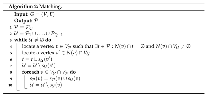
The general procedure is described in Algorithm 2. It needs all the partitions obtained in Algorithms 1, and 2 adequately pastes them.

Let ${\mathcal{P}}_Q$ be the partition of $B_Q$ obtained in Algorithm 1. Let $\mathcal{U}={\cup }_{i=1}^{Q-1}{\mathcal{P}}_i$ be the union of the rest of the partitions from Algorithm 1. Let $V_{{\mathcal{P}}_Q}={\cup }_{t\in {\mathcal{P}}_Q}t$ be the set of nodes of the ${\mathcal{P}}_Q$ elements and let $V_{\mathcal{U}}={\cup }_{t\in \mathcal{U}}t$ be the set of nodes of the $\mathcal{U}$ elements. For each v in V and each set $\mathcal{P}$ of sets of $V,$ let $s_{\mathcal{P}}\left(v\right)$ be a set in $\mathcal{P}$ that contains node $v.$ Algorithm 2 reads as follows.

Proposition 6.

While Algorithm 2 does not finish (while $\mathcal{U}\ne \varnothing$), it is possible to locate a vertex $v\in {\nu }_{\mathcal{P}}$ such that there exists a $t\in \mathcal{P}:N\left(v\right)\cap t=\varnothing$ and $N\left(v\right)\cap {\nu }_{\mathcal{U}}\ne \varnothing$, and also to locate a vertex $v^{\prime }\in N\left(v\right)\cap V_{\mathcal{U}}$ (lines 4 and 5 of Algorithm 2).

Proof. 

On the one hand, if there were no $t\in \mathcal{P}:N\left(v\right)\cap t=\varnothing$, that would mean the domatic partition has already been found. On the other hand, if there were $t\in \mathcal{P}:N\left(v\right)\cap t=\varnothing$ but $N\left(v\right)\cap {\nu }_{\mathcal{U}}=\varnothing$, that would mean it is not possible to find a domatic partition of G, which cannot happen according to the Propositions 4 and 5. □

Proposition 7.

Algorithm 2 gets a domatic partition of G from the partitions of the blocks provided by Algorithm 1.

Proof. 

First of all, note that $\mathcal{P}$ always has a domatic number of subsets. Second, since the algorithm successively finds a node v in $\mathcal{P}$ that is not dominated by a subset t, and given that according to Proposition 6 it is possible to incorporate into t a subset in $\mathcal{U}$ that dominates $v,$ then the Algorithm 2 obtains a domatic partition of G. □

Proposition 8.

Algorithm 1 returns a domatic partition of G.

Proof. 

Given that Algorithm 1 calls Algorithm 2, providing it with $d\left(G\right)$ allied domatic partitions of each block in $G,$ then according to Proposition 7, a domatic partition of G is obtained. □

4. Computational Experience

We carried out a computational experience in order to analyse the performance of the decomposition method proposed to compute the domatic partition in graphs with blocks. We tested our techniques over a set of 117 randomly generated instances. Specifically, these instances contain from 100 to 400 nodes, progressively increasing the size from 25 to 25, that is, 100, 125, …, 400 nodes. In turn, it generated nine different instances for each one of these node sizes, according to the densities $1.5$, $2.5$, $5.0$, $7.5$, $10.0$, $12.5$, $15.0$, $17.5$ and $20.0$. That is, we have nine instances of 100 nodes, and respectively 150, 250, 500, 750, 1000, 1250, 1500, 1750, 2000 edges; nine instances of 125 nodes and respectively 188, 313, 625, 938, 1250, 1563, 1875, 2188 and 2500 edges; and so on. Apart from the randomness employed to generate these instances, they were generated in such a way that a Hamiltonian cycle can be found in every one. Finally, each one of them were joined up with itself from the initial node in such a way that the final instances have two symmetrical blocks and they cover from 199 to 799 nodes progressively, increasing the sizes from 50 to 50.

Our experiments were conducted on a PC with a 2.60 GHz Intel Xeon, 64 GB of RAM, and Ubuntu 18.04.5 LTA operating system. The instances were solved twice by linear integer programming, using both the general method and the decomposition approach. To solve the linear integer models, we used the optimisation engine IBM ILOG CPLEX Interactive Optimiser 20.1.0.0, setting a max computing time per instance of 3600 s.

Table 2. Times of concluded instances by nodes.

Nodes	# Solved	DP Time	Algorithm 1 Time
199	7	13.29	2.86
249	8	322.12	96.50
299	7	118.14	41.43
349	6	513.17	50.67
399	6	4.67	1.00
449	7	236.43	107.71
499	7	516.43	10.57
549	6	521.67	4.67
599	5	0.60	0.00
649	5	0.20	0.80
699	5	0.80	0.00
749	5	0.80	0.00
799	6	390.33	9.33
Average		216.98	28.49

summarises the computational processing times grouped by nodes of the instances that were concluded by both methods during the processing time limit. Column # solved shows the number of nine instances solved both by the DP model and by Algorithm 1. Column DP time shows the average time in seconds it took to solve the model (DP), that gives the domatic number $d\left(G\right)$ and the domatic partition. Column Algorithm 1 time shows the average time in seconds it took to solve Algorithm 1, that also gives $d\left(G\right)$ and the partition. The last row shows the global average for both methods, which is clearly advantageous for the decomposition approach, with an average time of $28.49$ s versus $216.98$ s of the general method. The more prominent advantage was obtained in the instances of 549 nodes which needed an average of $521.67$ s to be solved by the optimisation model approach, whilst the decomposition approach only required an average of $4.67$ s.

Instances with 599 to 749 nodes may seem easy instances due to the average times listed. However, the fact is that a lot of instances of these groups did not conclude, and therefore only the times of the easy instances were taken into account. In this respect,

Table 3. Number of non-concluded instances by nodes.

Nodes	DP Model	Algorithm 1
199	2	2
249	1	1
299	2	2
349	3	3
399	3	2
449	2	1
499	2	1
549	3	2
599	4	2
649	4	3
699	4	4
749	4	2
799	3	3
Total	37	28

provides information about the instances that have not been completed for each group and method. The DP model could not solve 37 of the 117 instances within the time limit, whilst the instances not solved by the decomposition method were 28. Note how only five of the nine instances for the groups of 599 to 749 nodes were solved by the general method. Finally, the major advantage of the decomposition approach was obtained in the group of 599 instances where the decomposition method solved seven instances, whilst the general only solved five.

The instances that Algorithm 1 could not complete were not concluded by the DP model either. Conversely, there were nine instances concluded by the decomposition approach that could not be concluded by the DP model. The details of each one of these last instances are shown in

Table 4. Detail of non-concluded instances.

# Nodes	# Edges	LB (DP)	$\mathit{d}\left(\mathit{G}\right)$	Time
399	6000	8	8	2634
449	7876	6	8	1872
499	8750	7	8	1994
549	8250	6	8	3442
599	7500	5	6	2300
599	9000	6	7	2664
649	9750	5	6	2
749	9376	5	5	2
749	15,000	6	8	6

. Columns # nodes and # edges respectively indicate the number of nodes and edges of each instance, $LB\left(DP\right)$ the value of the best feasible solution found by the DP model, $d\left(G\right)$ the optimal value found by Algorithm 1, and finally, Column time indicates the solution time employed by Algorithm 1. Note that the best feasible solution found by the DP model just coincides with the optimal solution in the first instance. We also highlight that the solution time for the three last instances is very small.

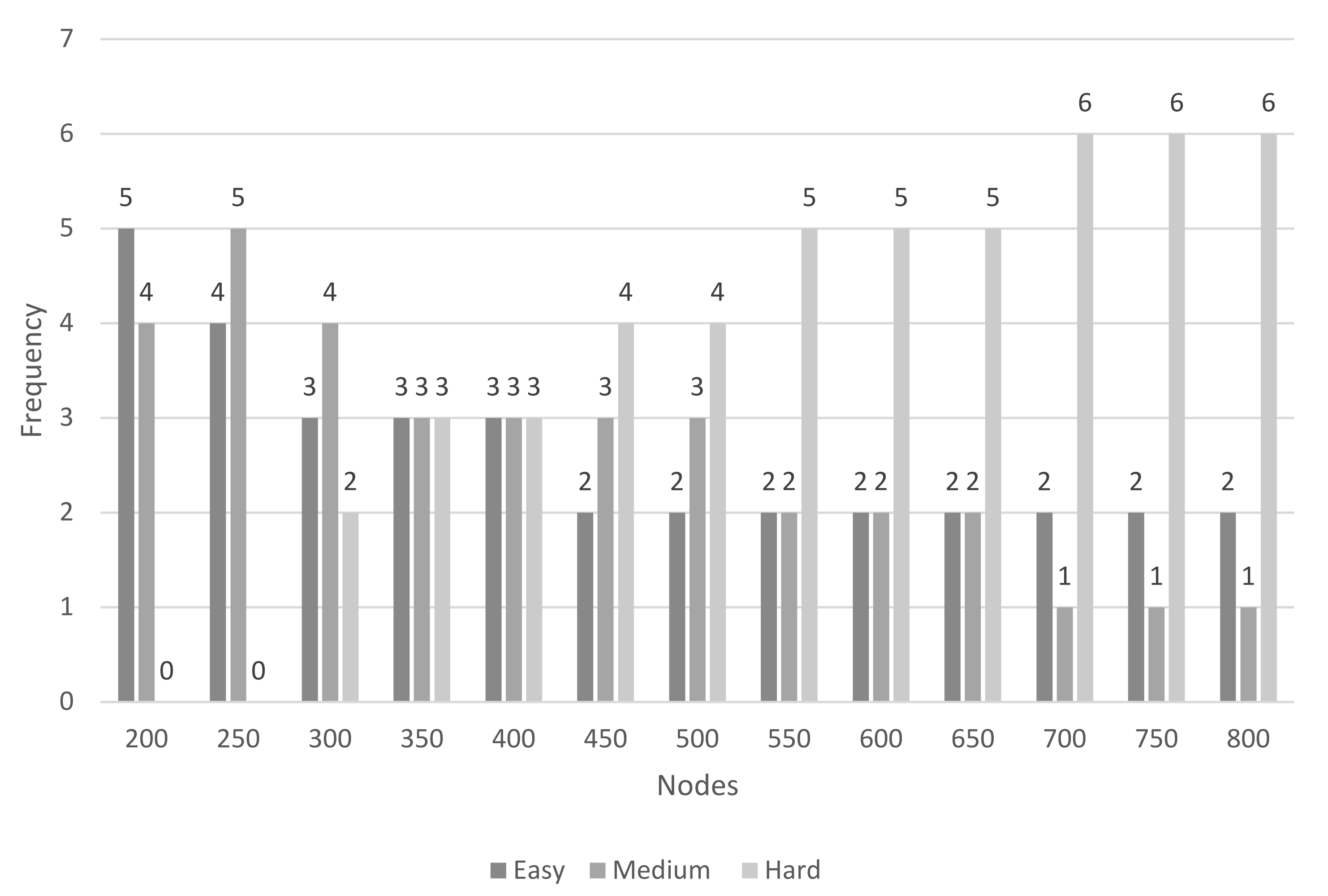
Given that the processing difficulty of the instances is more correlated to the number of edges than to the number of nodes, we have also obtained several tables summarising the results according to their number of edges. We classify the instances into three groups: easy, medium and hard.

Table 5. Classification of computational hardness.

Difficulty	Edges	# Instances
Easy	≤2000	34
Medium	2001–5000	34
Hard	≥5001	49
Total		117

shows the criteria followed to classify the instances according to the number of edges, as well as the number of instances belonging to each level of computational hardness.

There are easy instances with any number of nodes, but there are hard instances with only 300 nodes or more. Figure 6 shows the frequency of each type of instance for each number of nodes.

Table 6. Times of concluded instances by computational hardness.

Difficulty	DP Model	Algorithm 1
Easy	2.68	0.63
Medium	210.55	44.71
Hard	716.00	60.00
Average	216.98	28.49

and

Table 7. Number of non-concluded instances by computational hardness.

Difficulty	DP Model	Algorithm 1
Easy	0	0
Medium	3	3
Hard	34	25
Total	37	28

aggregate the information in Table 2 and Table 3 respectively by difficulty. The former gives the average time, and the second, the number of unsolved instances. The last rows (average and total) coincide with the last rows in Table 2 and Table 3. Observe that the DP model did not solve 34 of the 49 hard instances, whilst Algorithm 1 did not solve 25 of them.

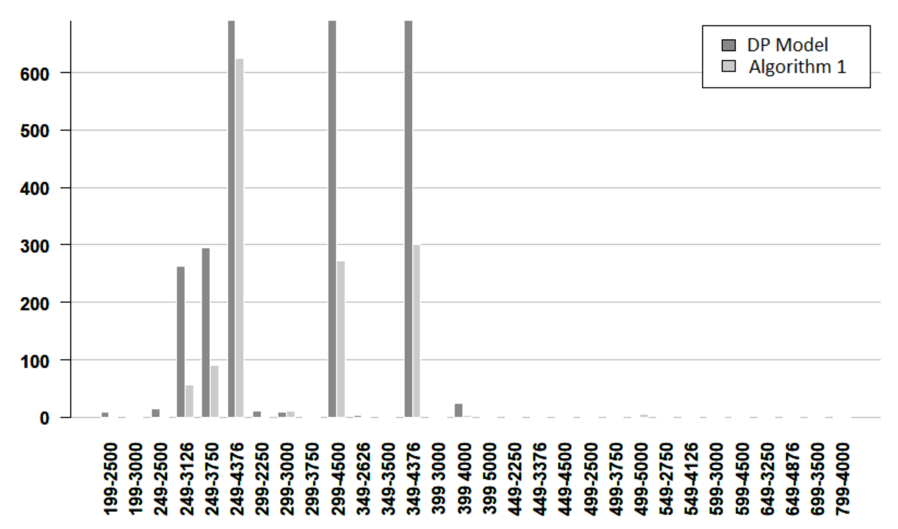
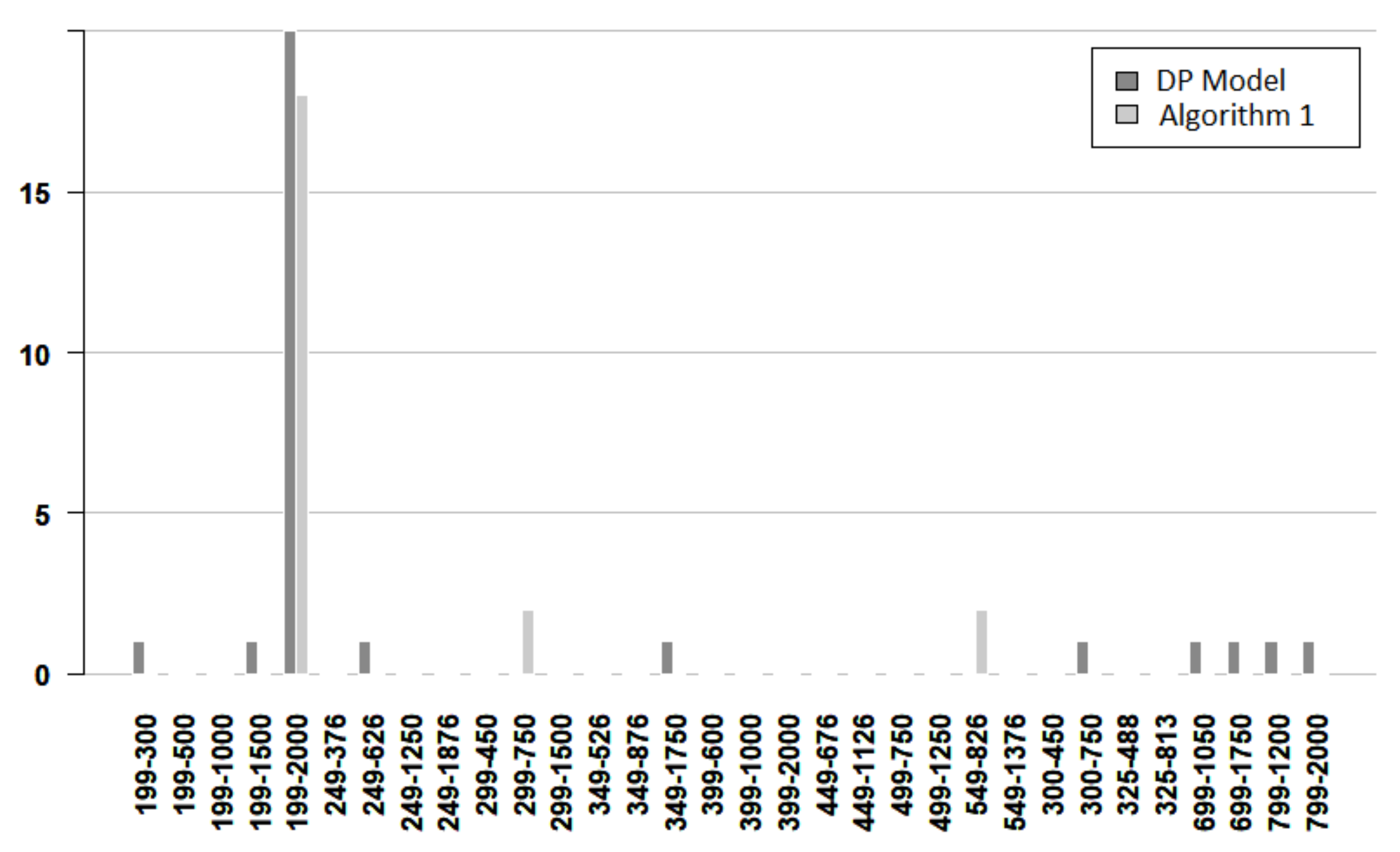
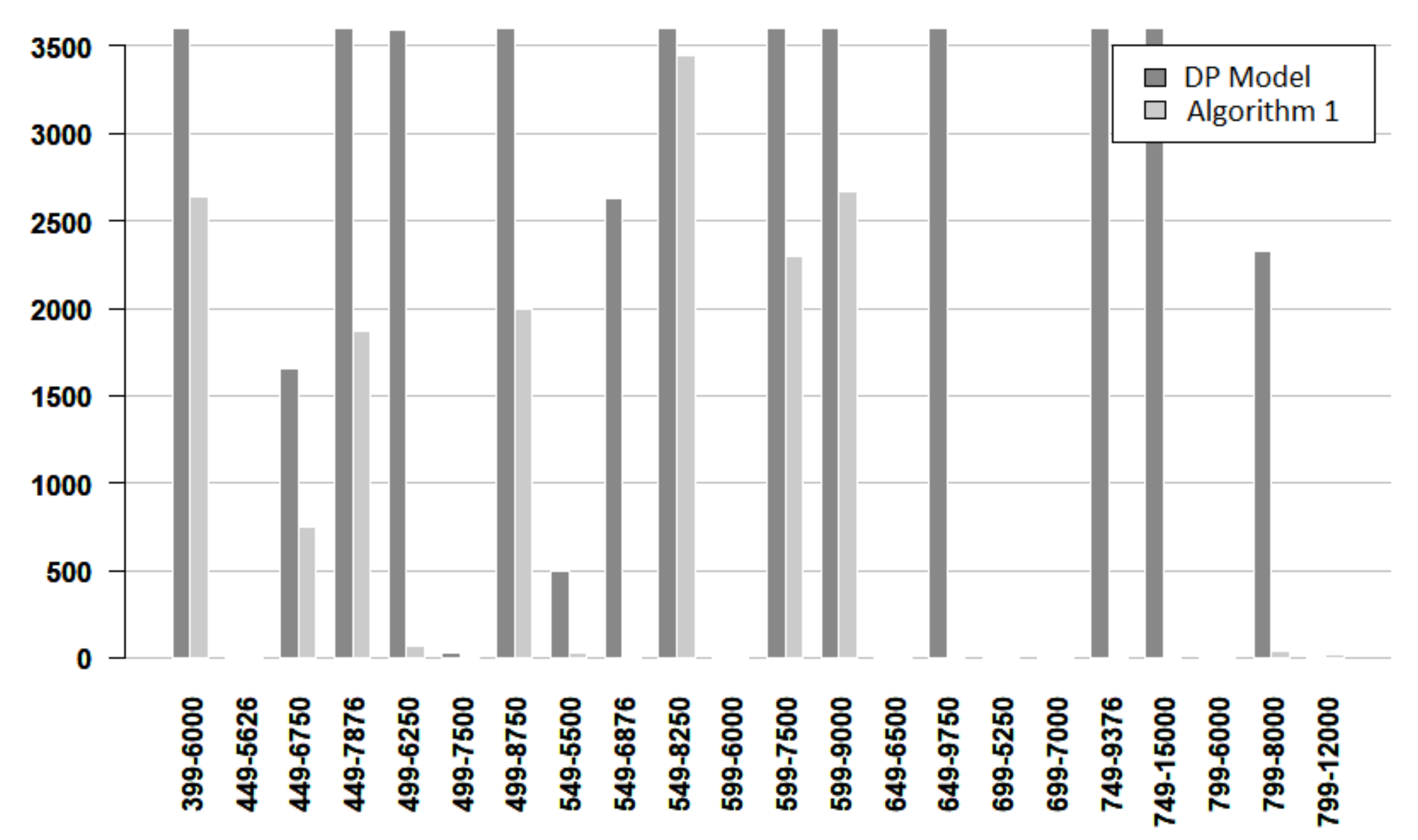
Figure 7, Figure 8 and Figure 9 give more details about the resolution time for solving the DP model and Algorithm 1. The vertical axis denotes the time and the horizontal axis indicates the instance. Each instance is named by its number of nodes and its number of edges. From these figures, it follows that most of the easy instances are solved in less than 5 s, and there are more DP bars than Algorithm bars. For easy instances, only one instance required more than 5 s, and the algorithm used less time for concluding. For medium instances, most of the times are very small, but when the time is larger than 10 s, the algorithm works faster. For hard instances, the bars for the DP model are always larger than the bars for the algorithm. Furthermore, in some cases, the algorithm time bar is negligible, while the DP time bar exceeds 2000 s.

5. Conclusions and Future Research

In this paper, we have introduced a new generalisation of domination named allied domination. Our motivation for its introduction was to improve the computational effort to calculate the domatic partition of a graph, and as a consequence, its domatic number by decomposing a graph into its blocks. An exact method for calculating the domatic partition is the major contribution of this paper. In addition, it is supported by extensive computational experience measuring its advantages.

On the one hand, future works can be focused on extending and deepening allied domination. Its properties can be studied by using both exact and approximation techniques. On the other hand, heuristic and approximation algorithms can also be developed in order to calculate not only the domatic number, but also related problems by taking advantage of the knowledge provided by the decomposition exact method proposed.