Beam-Influenced Attribute Selector for Producing Stable Reduct

Abstract

Attribute reduction is a critical topic in the field of rough set theory. Currently, to further enhance the stability of the derived reduct, various attribute selectors are designed based on the framework of ensemble selectors. Nevertheless, it must be pointed out that some limitations are concealed in these selectors: (1) rely heavily on the distribution of samples; (2) rely heavily on the optimal attribute. To generate the reduct with higher stability, a novel beam-influenced selector (BIS) is designed based on the strategies of random partition and beam. The scientific novelty of our selector can be divided into two aspects: (1) randomly partition samples without considering the distribution of samples; (2) beam-based selections of features can save the selector from the dependency of the optimal attribute. Comprehensive experiments using 16 UCI data sets show the following: (1) the stability of the derived reducts may be significantly enhanced by using our selector; (2) the reducts generated based on the proposed selector can provide competent performance in classification tasks.

1. Introduction

In the era of big data and artificial intelligence, the scale of data is growing massively [1]. Without loss of generality, high dimensionality has become one of the crucial characteristics of modern data [2]. For data analyses related to practical applications [3,4], such a characteristic may bring us huge challenges, which can be divided into the following two phases: (1) in the process of data production, redundant or irrelevant dimensions may lead to the low quality of data; (2) the storage and processing of data are facing tremendous difficulties because of the interference influenced by the numerous dimensions. Therefore, how to reasonably reduce the dimensions of data has become an urgent problem to be addressed.

As one of the effective technologies for realizing dimension reduction, feature selection [5,6,7,8] has been widely explored. Different from some other dimension reduction technologies, such as feature extraction, the aim of feature selection is to determine some informative features and then select them from the original features. Through using feature selection, it is expected that the selected features will provide better readability and interpretability [9,10] for the learning models. Presently, with respect to diverse requirements, various approaches with respect to feature selection are developed. Among most of the popular results, it is noteworthy that rough-set-based feature selection has been paid much attention. The reasons can be attributed to the following superiorities: (1) clear semantic explanation for such a technique is useful in terminating the process of feature selection; (2) the extensibility of rough set theory is extremely important because it offers us rich measurements for evaluating the significance of features.

Concerning rough-set-based feature selection, the output is frequently referred to as the reduct because such a feature selection is firstly named as attribute reduction by Pawlak [11] in the theory of rough set [11,12,13,14]. Through reviewing numerous results with respect to attribute reduction, it can be observed that most of the research is motivated by either the time efficiency of seeking the reduct or the generalization ability of the obtained reduct [15,16,17,18]. Nevertheless, to the best of our knowledge, few of the studies take the data perturbation into account. In other words, the stability of the obtained reduct [19,20] is seldom considered.

The stability of the reduct is defined as “sensitivity of reducts generated by an algorithm to the differences of training sets drawn from same generation distribution”. In simple terms, the reduct stability reflects the varying degree of reducts when data perturbation happens. The reduct with higher stability will bring us stable learning results, and it can enhance the confidence of domain experts when experimentally validating the selected attributes to interpret important discoveries. It is obvious that stability is one important metric for evaluating the performance of derived reducts. Therefore, the main research problem of this study is how to generate the reduct with higher stability when data perturbation happens.

In view of searching for a stable reduct, Yang and Yao [21] have firstly designed a naive ensemble selector. Though the framework of such a selector is rough, the multiple perspectives [22,23] for determining attributes with better adaptability have been preliminarily reported. Immediately, the reduct generated by using an ensemble selector may be more robust than those obtained by previous research.

However, through a critical review of the results related to ensemble selectors, some limitations may be easily revealed: (1) such a selector relies heavily on the distribution of samples; (2) such a selector also relies heavily on optimal attributes of each perspective. The former indicates that the multiple perspectives in the ensemble selector are constructed based on the distribution of samples. From this point of view, the critical requirement of following the raw distribution may greatly limit the applications of ensemble selectors in complex data. The latter implies the determination of the best attributes for each iteration in the mechanism of an ensemble selector. Therefore, the locally optimal solution instead of the globally optimal solution may be derived.

By considering the above limitations and the requirement of deriving a stable reduct, a beam-influenced attribute selector will be designed in the context of this paper. Such a selector contains two main keys: (1) randomly partition the samples [24], it can be regarded as the source of multiple beams; (2) add two or more potential attributes into each beam [25]. Therefore, different from the conventional ensemble selector, our selector is neither required to preserve the raw distribution of samples because the random partition over samples is employed nor asked to determine one and only one satisfactory attribute in each iteration because the beam is used to record multiple candidate attributes. Immediately, it is obvious that our beam-influenced attribute selector presents two different perspectives of the ensemble, one is from the perspective of the sample and the other is from the perspective of attributes. Therefore, more bases for realizing ensemble selection can be obtained and then the attribute with stronger adaptability can be determined. This is the inherent reason that our beam-influenced attribute selector may output a stable reduct.

The contribution of this study can be divided into the three phases as follows. Firstly, through analyzing the framework of an ensemble selector, some limitations of this framework are revealed. These limitations can be summarized into two aspects: (1) rely heavily on the distribution of samples; (2) rely heavily on the selection of optimal features. Secondly, to overcome these limitations in the ensemble selector, a novel beam-influenced selector (BIS) is developed. Finally, through the observation and analysis of extensive experimental results, it is verified that our selector can be effectively used to generate stable reducts, and these reducts generally possess competent classification performance.

The remainder of this paper is organized as follows. In Section 2, some basic concepts with respect to attribute reduction and measurement of stability are introduced briefly. In Section 3, ensemble selector-based attribute reduction and beam-influenced selector-based attribute reduction are presented elaborately. In Section 4, experimental results and corresponding analyses are reported clearly. Finally, some conclusions and suggestions for future work are offered in Section 5.

2. Preliminaries

2.1. Attribute Reduction

Currently, the relationship between attributes and labels not only provides guidance for constructing various attribute reduction-related constraints [11,26,27,28] in the field of attribute reduction [29,30,31] but also suggests positive heuristic information for generating a reduct based on appropriate attributes.

Up to now, it is well-known that many relationships and the corresponding constraints have been thoroughly explored and that the forms of attribute reduction vary considerably [32,33,34,35]. Different reducts possess different semantic explanations, which are closely determined by the used relationships.

However, though the forms of relationships and constraints are rich in previous research, it must be noted that the essence of attribute reduction can be further abstracted. Such an abstraction can not only reveal the clear framework of attribute reduction but also provide a broad space for introducing popular techniques into the study of attribute reduction-related topics. The following Definition 1 shows us a detailed abstraction [15].

Definition 1.

[36] Given a decision system $\mathcal{DS}=⟨U,AT\cup \left\{d\right\}⟩$, in which $AT$ and U are nonempty finite sets with respect to condition attributes and all samples, d is the decision attribute. Suppose that ${\mathcal{C}}_{\rho }^U$ is a constraint associated with a pre-defined measure ρ, $\forall A\subseteq AT$, A is considered as a ρ-reduct if and only if the following conditions are satisfied:

(1) 

A holds the constraint ${\mathcal{C}}_{\rho }^U$;

(2) 

$\forall B\subset A$, B does not hold the constraint ${\mathcal{C}}_{\rho }^U$.

In Def. 1, $\rho$ can be considered as a function that can map $P\left(U\right)\times P\left(AT\right)$ to a set of real numbers $\mathcal{R}$, where $P(.)$ is an operation of the power set.

Immediately, the natural problem is how to generate the satisfactory reduct. Because of its low time complexity, the heuristic-based greed searching strategy is paid much attention to. Most of the greedy searchings [30,37,38] can be grouped into the following three phases.

(1)

Forward greedy searching. For each iteration, one or more appropriate attributes can be selected based on the evaluations of the candidate attributes. Thereby, through using sufficient iterations, a satisfactory reduct can be generated.

(2)

Backward greedy searching. For each iteration, one or more inferior attributes will be removed from the set of the raw attributes based on the evaluations. Then, through using sufficient iterations, a justifiable reduct can also be obtained.

(3)

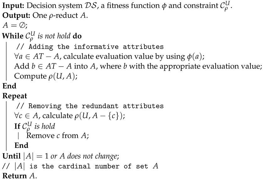
Forward-Backward greedy searching. In such a strategy, both the forward and backward strategies are employed for seeking a reasonable reduct. For example, firstly, a potential reduct can be generated based on the strategy of forward searching; secondly, the redundant attributes in such a potential reduct can be further removed by the backward searching.

Among the above strategies, forward-backward greedy searching is the well-trodden strategy. The reasons can be summarized as follows: such strategy not only guarantees that the informative attributes are added into the potential reduct preferentially but also makes sure that there are no redundant attributes in the obtained reduct. The details of forward-backward greedy searching are presented as follows.

In Algorithm 1, $\forall a\in AT$, the fitness value will be calculated by using the fitness function $\varphi$ ($\varphi$ map a to the set of real numbers) that can quantitatively characterize the significance of each candidate attribute. It must be pointed out that the fitness function is generally associated with the measure $\rho$ [36].

Algorithm 1: Forward-backward greedy searching for attribute reduction (FBGSAR).

2.2. Measurement of Stability

Following the above discussions, testing the performances of the derived reduct is an inevitable problem. In addition to generalization performances related to classifiers, the stability of the derived reduct is another performance that should be paid attention [21].

For instance, suppose that data perturbation results in significant variations of the reducts, it means that the generated reducts are unstable. Obviously, unstable reducts will lend to unstable results of learning.

In this paper, the stability represents the degree of reduct perturbation when data perturbation happens. From this point of view, the reduct stability [39,40] is defined as Definition 2.

Definition 2.

[21] Given a decision system $\mathcal{DS}$, if U is split into $U_1,U_2,\dots ,U_m$ ($|U_1|=|U_2|=\cdots =|U_m|$), then the stability of the reduct is

$${\mathrm{Sta}}_{\mathrm{Reducet}}=\frac{1}{m(m-1)}\sum _{i=1}^m\sum _{j=1,j\ne i}^m\frac{|A_i\cap A_j|}{|A_i\cup A_j|},$$

(1)

where $A_i$ is the reduct obtained over $U-U_i$.

3. Beam-Influenced Selector for Attribute Reduction

3.1. Ensemble Selector for Attribute Reduction

As shown in Algorithm 1, each candidate attribute is evaluated based on a single fitness function. Nevertheless, it is well-known that a single fitness function will bring the following challenges [41].

(1)

Single fitness function may lead to poorer adaptability. For example, a reduct generated based on a single granularity may fail to qualify as the reduct over other granularity, such as a slightly finer or coarser granularity [41] generated by a slight data perturbation.

(2)

Single fitness function may result in a poorer learning performance. For instance, in different classes, samples possess some distinct characteristics [31] that tend to optimize class-specific measurements. Nevertheless, revealing the differences among these differentiated characteristics using merely one fitness function is quite challenging.

To overcome the limitations mentioned above, a representative ensemble selector based attribute reduction has been designed by Yang and Yao [21]. Different from Algorithm 1, a set of fitness functions is used in the ensemble selector for evaluating each candidate attribute. The detailed process of the searching reduct based on the ensemble selector is shown as follows.

Actually, the fitness function is designed to measure the significance of each candidate attribute. Therefore, different perspectives can be constructed by using different fitness functions. For such a reason, the fitness function sets used in Algorithm 2 can be grouped into the following two broad categories.

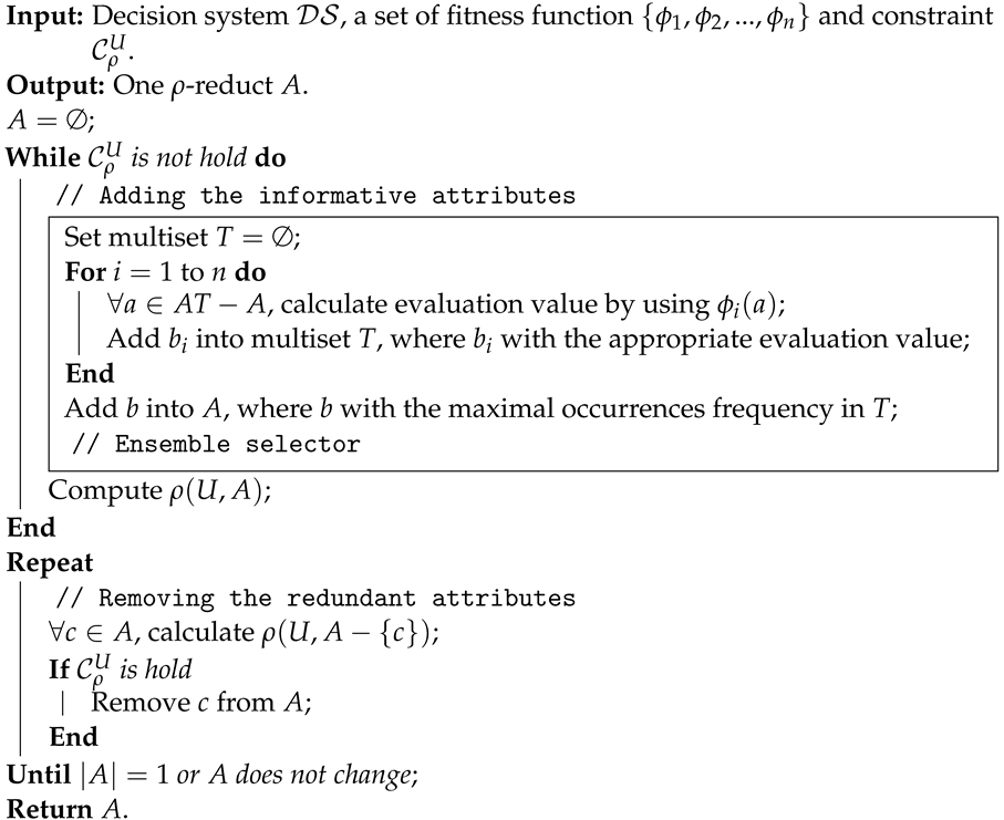
(1)

Homogenous fitness function set: the set of fitness function {${\varphi }_1,{\varphi }_2,\dots ,{\varphi }_n$} is constructed using same evaluation criterion. For instance, the fitness function set can be defined based on approximation qualities of different rough set models, and then the generated can better adapt to different models.

(2)

Heterogeneous fitness function set: the set of fitness function {${\varphi }_1,{\varphi }_2,\dots ,{\varphi }_n$} is built using different evaluation criteria. For example, the fitness function set can be defined based on many different measures of a rough set model, such as approximation quality and entropy, etc., and then, the derived reduct will better adapt to different constraints.

Algorithm 2: Ensemble selector-based attribute reduction (ESAR).

Algorithm 2 has substituted the set of fitness functions for a single fitness function. Therefore, compared with the conventional approach, the ensemble selector-based strategy may effectively improve the stability of the obtained reducts. The crucial reason is that the candidate attributes can be evaluated based on multiple perspectives, which makes the selected attributes may be equipped with more adaptability and generality.

Following the basic principle of Algorithm 2, some different forms of ensemble selectors [21,41,42] have also been investigated. However, it must be pointed out that most of these results suffer from a couple of limitations shown as follows.

(1)

Rely heavily on the distribution of samples. Take the classical ensemble selector proposed by Yang and Yao [21] as an example; each fitness function is constructed based on the samples with the same label. Therefore, the performance of the used fitness functions will be degraded if sample distribution is seriously unbalanced or the categories of samples are fewer.

(2)

Rely heavily on the selection of appropriate features. Take the selector proposed by Jiang et al. [42] as an example, only the optimal attribute will be selected based on each fitness function. Therefore, some candidate attributes with potential importance will be ignored, which indicates that some attributes with strong adaptability will be difficult to determine.

3.2. Beam-Influenced Selector-Based Attribute Reduction

Considering what has been pointed out in the above subsection, those limitations may lead to poor adaptability of the selected attributes. Motivated by this, two strategies called random partition [24] and beam [25] are employed in our attribute selector. The detailed structure of the beam-influenced selector (BIS) is shown in the following Figure 1.

Figure 1. The framework of beam-influenced selector (BIS).

The details of our beam-influenced selector (BIS) shown in Figure 1 can be elaborated as follows:

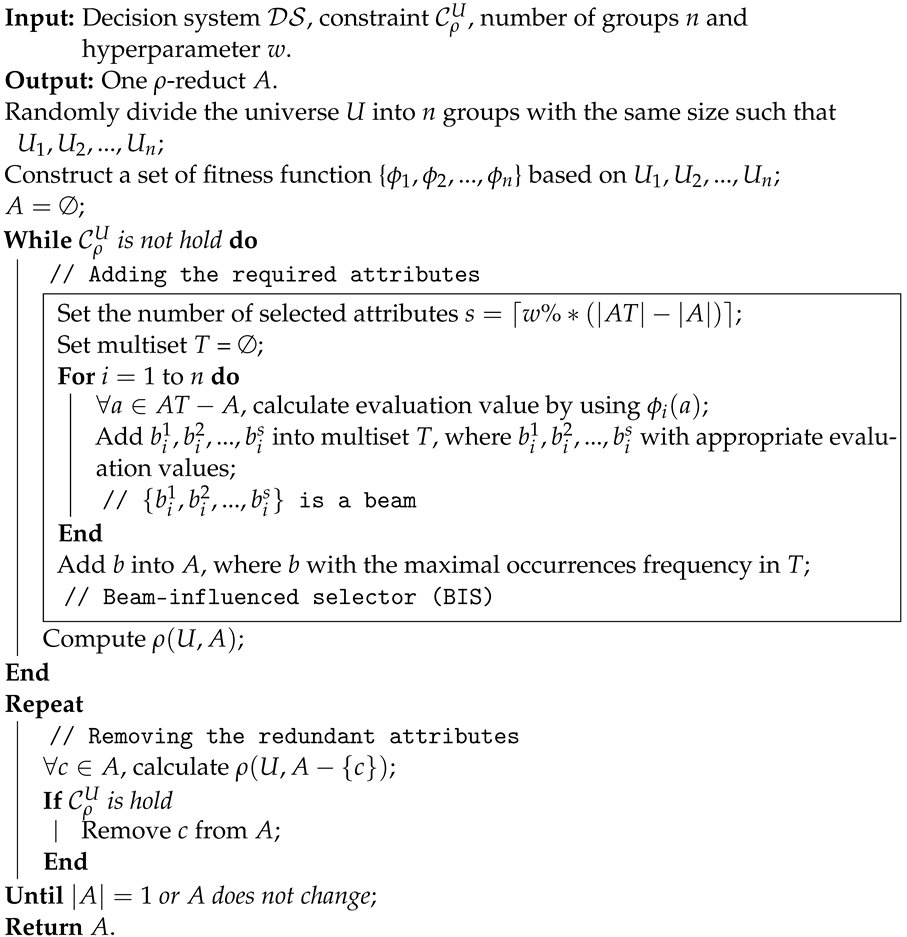
(1)

Divide the set of raw data into $n(n\in \{1,2,\dots ,\lceil \left|u\right|/5\rceil \left\}\right)$ groups in terms of the samples;

(2)

Different fitness functions ${\varphi }_1,{\varphi }_2,\dots ,{\varphi }_n$ are constructed based on different n groups of samples;

(3)

Each candidate attribute can be evaluated by different fitness functions, and then the top $w\%(0<w\le 50)$ of the attributes with respect to the evaluation results over each fitness function will be added into the multiset T;

(4)

Select an attribute b with the maximal frequency of occurrences in the multiset T.

Following the above discussions, our searching strategy may be equipped with the following superiorities. Firstly, it will not be influenced by the distribution of samples. This is mainly because the whole universe is randomly partitioned into n different groups and then the distribution of each local datum is not the key thing that should be paid the most attention. Secondly, more important attributes will be considered and added into the multiset T. Those attributes are determined by not only various local data-based fitness functions but also the beam-based top $w\%$ selection related to each local data. Immediately, the attribute with stronger adaptability may be selected for each iteration.

The following Algorithm 3 shows the specific process of deriving a reduct based on our beam-influenced selector.

Algorithm 3: Beam-influenced selector-based attribute reduction (BISAR).

In Algorithm 3, the set of homogeneous fitness functions is used, principally because: (1) those different fitness functions correspond to the local data derived from the random partition over the raw data; (2) although the local data are different, the evaluation mechanisms over those local data are same.

Compared with previous studies, it is obvious that the number of ensemble members can be adjusted freely by both the number of local data/fitness functions and the number of the beam-based top attributes. Put another way, each candidate attribute can be fully evaluated by more views. As a result, it is expected that the reduct generated by using Algorithm 3 may have a higher stability.

4. Experimental Analysis

4.1. Data Sets and Configuration

For verifying the validity and superiority of the proposed strategy, experimental comparisons are conducted in this section. All experiments were carried out on a personal computer with Windows 10, AMD 3750 (2.60 GHz) and 4.00 GB memory. The programming language is Matlab R2018b. Classifier packages (fitcecoc, fitcknn) used in the experiment are from the software of Matlab. The total run time of all experiments was about one month. Furthermore, Table 1 summarizes details of 16 UCI data sets that were used in our experiments.

Table 1. Data sets description.

ID	Data Sets	Samples	Attributes	Decision Classes
1	Breast Cancer Wisconsin (Diagnostic)	569	30	2
2	Breast Tissue	106	9	6
3	Congressional Voting Records	435	16	2
4	Forest Type Mapping	523	27	4
5	Ionosphere	315	34	2
6	LSVT Voice Rehabilitation	126	256	2
7	Lymphography	98	18	3
8	Madelon	2600	500	2
9	Musk (Version 1)	476	166	2
10	Parkinsons	195	23	7
11	Parkinson Speech Dataset with Multiple Types of Sound Recordings	1208	26	2
12	QSAR biodegradation	1055	41	2
13	Sonar	208	60	2
14	Statlog (Heart)	270	13	2
15	Synthetic Control Chart Time Series	600	60	6
16	Wine	178	13	3

4.2. Experimental Setup

The model that was used for deriving reducts during our experimentations is the neighborhood rough set [26,43]. Note that the results obtained using the neighborhood rough set model are closely dependent on the given radius. For such reason, to verify the universality of BIEAR, 20 radii were selected for the experiment; these are 0.02, 0.04, …, 0.40 [15,24,44].

Furthermore, the 5-fold cross-validation was applied for searching reducts. The strategy of 5-fold cross-validation will divide the whole samples into 5 disjoint groups, i.e., $U_1,U_2,\dots ,U_5$. For the first round of computation, $U_1\cup \cdots \cup U_4$ is considered as the set of training samples for searching for the reduct and then $U_5$ is considered as the set of testing samples for evaluating performances with respect to the generated reduct; …; $U_2\cup \cdots \cup U_5$ is considered as the set of training samples to search for the reduct and then $U_1$ is considered as the set of testing samples for evaluating performances with respect to the generated reduct [44]. Therefore, the experimental studies reported in this paper are quite reliable and aim to provide a solid basis for a thorough evaluation of BISAR’s effectiveness.

Moreover, it is worth noting that besides the above raw data sets, two types of noise have also been injected into the raw data for further testing the effectiveness of our BISAR.

(1)

Feature noise. Given raw data, if the noise ratio is $\omega \%$, then the injection is realized by randomly selecting $\omega \%(0<\omega <100)$ features and replacing the values over these features with random numbers (value range is [0, 1]).

(2)

Label noise. Given raw data, if the noise ratio is $\omega \%$, then the injection is realized by randomly selecting $\omega \%(0<\omega <100)$ samples and replacing the labels of these samples randomly.

Finally, the feature noise ratio and the label noise ratio are set as 20%, the hyperparameters n and w of BISAR are set as 20. The following five strategies for obtaining reducts are also reproduced for comparing with our BISAR.

(1)

Attribute group based attribute reduction (AGAR) [15];

(2)

Dissimilarity based attribute reduction (DAR) [45];

(3)

Data-guidance based attribute reduction (DGAR) [42];

(4)

Ensemble selector-based attribute reduction (ESAR) [21];

(5)

Forward-backward greedy searching based attribute reduction (FBGSAR) [15].

4.3. Comparisons of Stability-Based Reducts

In this subsection, the stabilities of different reducts driven by AGAR, DAR, DGAR, ESAR, FBGSAR and our proposed strategy will be compared. The stability is reflected by how data perturbation will influence the reduct. Therefore, stabilities of reducts obtained by different strategies can be computed based on 5-fold cross-validation. The computation of stability has been shown in Equation (1). Since 20 different radii are used to obtain reducts in our experiments, the following Table 2, Table 3 and Table 4 show us the mean value of stabilities based on 20 different reducts.

Table 2. The stabilities of reducts (raw data).

ID	AGAR	DAR	DGAR	ESAR	FBGSAR	BISAR
1	0.5116	0.6466	0.6446	0.5295	0.5830	0.7501
2	0.7708	0.8025	0.8336	0.9329	0.7882	0.9522
3	0.4259	0.6850	0.4091	0.6378	0.4116	0.6158
4	0.6150	0.7408	0.6306	0.7412	0.6316	0.8098
5	0.2807	0.3978	0.3669	0.4608	0.3340	0.6511
6	0.1103	0.2194	0.1133	0.1380	0.1133	0.6188
7	0.3868	0.6086	0.4620	0.5804	0.3790	0.7739
8	0.1938	0.5297	0.2558	0.1617	0.2863	0.2903
9	0.1539	0.3790	0.1835	0.1644	0.1720	0.4745
10	0.6410	0.7520	0.6732	0.7808	0.7015	0.9089
11	0.7343	0.8704	0.7937	0.7795	0.7897	0.8321
12	0.6175	0.8238	0.7584	0.7340	0.7504	0.8561
13	0.1176	0.2981	0.1360	0.1773	0.1360	0.4064
14	0.6271	0.7977	0.7885	0.7137	0.7279	0.8033
15	0.2442	0.4187	0.3343	0.5237	0.3503	0.3575
16	0.4448	0.6289	0.4940	0.5229	0.5821	0.6984
avg	0.4297	0.5999	0.4924	0.5362	0.4835	0.6750

Table 3. The stabilities of reducts (label noise).

ID	AGAR	DAR	DGAR	ESAR	FBGSAR	BISAR
1	0.5848	0.7555	0.6281	0.6193	0.6262	0.8081
2	0.7636	0.8302	0.7845	0.9234	0.7816	0.9458
3	0.7114	0.7385	0.7082	0.7228	0.7190	0.8988
4	0.6567	0.7937	0.6703	0.7292	0.6828	0.8493
5	0.4669	0.5529	0.4509	0.5955	0.4665	0.8205
6	0.0600	0.1926	0.0650	0.0838	0.0792	0.5738
7	0.3840	0.5854	0.4474	0.4809	0.4648	0.8300
8	0.1577	0.4950	0.2119	0.1310	0.2023	0.2668
9	0.1066	0.3240	0.1345	0.1494	0.1372	0.5461
10	0.6341	0.7588	0.7009	0.8062	0.6779	0.9239
11	0.7193	0.8477	0.7675	0.7773	0.7747	0.8538
12	0.6279	0.7981	0.6976	0.7188	0.6961	0.8670
13	0.1342	0.3135	0.1434	0.1814	0.1585	0.4770
14	0.6935	0.8111	0.7675	0.7788	0.7881	0.8927
15	0.1679	0.3861	0.2522	0.3840	0.2597	0.3887
16	0.5738	0.6975	0.5854	0.6395	0.5768	0.8134
avg	0.4652	0.6175	0.5010	0.5451	0.5057	0.7347

Table 4. The stabilities of reducts (feature noise).

ID	AGAR	DAR	DGAR	ESAR	FBGSAR	BISAR
1	0.4297	0.5841	0.5316	0.4826	0.4832	0.7231
2	0.6788	0.7523	0.7252	0.8747	0.6940	0.9172
3	0.3373	0.5795	0.3602	0.5081	0.3810	0.5808
4	0.5410	0.7313	0.5629	0.6856	0.5901	0.7971
5	0.2081	0.2960	0.2529	0.3771	0.2445	0.5329
6	0.0787	0.1938	0.0851	0.1070	0.1127	0.6256
7	0.3359	0.5344	0.3956	0.5449	0.3918	0.7752
8	0.0988	0.4505	0.1116	0.0572	0.1012	0.1652
9	0.0906	0.3071	0.1104	0.1255	0.1104	0.4379
10	0.5575	0.6977	0.6098	0.7375	0.5988	0.8958
11	0.6398	0.8258	0.7298	0.7222	0.7209	0.7797
12	0.5395	0.7564	0.6436	0.6642	0.6498	0.8194
13	0.1001	0.2304	0.1114	0.1165	0.1148	0.4163
14	0.5740	0.7204	0.6593	0.6568	0.6500	0.7690
15	0.1659	0.3550	0.2281	0.4777	0.2168	0.3288
16	0.3641	0.5585	0.3889	0.4736	0.4165	0.6743
avg	0.3588	0.5358	0.4067	0.4757	0.4048	0.6399

Following Table 2, Table 3 and Table 4, it is not difficult for us to observe for following.

• Compared with reducts generated by AGAR, DAR, DGAR, ESAR and FBGSAR, the reduct obtained by our proposed strategy can possess higher stability in most cases over raw data. Take the “LSVT Voice Rehabilitation (ID: 6)” data set as an example, the values with respect to stabilities of reducts obtained by AGAR, DAR, DGAR, ESAR, FBGSAR and our proposed strategy are 0.1003, 0.2194, 0.1133, 0.1380, 0.1133 and 0.6188, respectively. It is obvious that the reduct with higher stability can be effectively generated by our BISAR.
• Whether the label noise data or feature noise data are considered, the reduct obtained by our proposed strategy can always possess high stability. Take “LSVT Voice Rehabilitation (ID: 6)” data set as an example, over the label noise data, the values with respect to stabilities of reducts obtained by AGAR, DAR, DGAR, ESAR, FBGSAR and our proposed strategy are 0.0600, 0.1926, 0.0650, 0.0838, 0.0792 and 0.5738; over the feature noise data, the values are 0.0787, 0.1938, 0.0851, 0.1070, 0.1127 and 0.6256. It is not difficult to draw a conclusion that our proposed strategy can better adapt to the data with label noise or feature noise.

In addition, the Wilcoxon signed rank test is employed to characterize the differences of the stability among several strategies, in which the significance level is appointed as 0.05. The results with respect to the Wilcoxon signed rank test are shown in the following Table 5, Table 6 and Table 7.

Table 5. p-values for comparing stabilities (raw data).

ID	AGAR and BISAR	DAR and BISAR	DGAR and BISAR	ESAR and BISAR	FBGSAR and BISAR
1	$1.7815\times {10}^{-3}$	5.3081 $\times {10}^{-2}$	7.6417 $\times {10}^{-2}$	1.5479 $\times {10}^{-2}$	4.9864 $\times {10}^{-2}$
2	3.9832 $\times {10}^{-6}$	6.7574 $\times {10}^{-8}$	4.6827 $\times {10}^{-10}$	8.0126 $\times {10}^{-1}$	8.1705 $\times {10}^{-5}$
3	6.6815 $\times {10}^{-8}$	7.8760 $\times {10}^{-8}$	7.8321 $\times {10}^{-9}$	5.4804 $\times {10}^{-5}$	7.9626 $\times {10}^{-9}$
4	9.7384 $\times {10}^{-3}$	3.6480 $\times {10}^{-1}$	1.0530 $\times {10}^{-2}$	9.3183 $\times {10}^{-2}$	6.0143 $\times {10}^{-3}$
5	2.2178 $\times {10}^{-7}$	6.7765 $\times {10}^{-8}$	7.5774 $\times {10}^{-6}$	3.6372 $\times {10}^{-3}$	3.2931 $\times {10}^{-5}$
6	6.0148 $\times {10}^{-7}$	6.7765 $\times {10}^{-8}$	9.1266 $\times {10}^{-7}$	7.5774 $\times {10}^{-6}$	2.6898 $\times {10}^{-6}$
7	6.7478 $\times {10}^{-8}$	3.4070 $\times {10}^{-7}$	2.0047 $\times {10}^{-7}$	5.2376 $\times {10}^{-4}$	6.1004 $\times {10}^{-8}$
8	2.3413 $\times {10}^{-3}$	6.7765 $\times {10}^{-8}$	3.2348 $\times {10}^{-1}$	5.0907 $\times {10}^{-4}$	5.2499 $\times {10}^{-1}$
9	2.0616 $\times {10}^{-6}$	6.7765 $\times {10}^{-8}$	6.6737 $\times {10}^{-6}$	2.0616 $\times {10}^{-6}$	4.5401 $\times {10}^{-6}$
10	7.8552 $\times {10}^{-5}$	8.1003 $\times {10}^{-2}$	7.0110 $\times {10}^{-5}$	2.9521 $\times {10}^{-3}$	2.1571 $\times {10}^{-4}$
11	1.3303 $\times {10}^{-2}$	4.3165 $\times {10}^{-3}$	2.7454 $\times {10}^{-2}$	1.6648 $\times {10}^{-2}$	2.0711 $\times {10}^{-2}$
12	1.9943 $\times {10}^{-4}$	3.1036 $\times {10}^{-1}$	4.6986 $\times {10}^{-3}$	2.2273 $\times {10}^{-3}$	7.1081 $\times {10}^{-3}$
13	9.1266 $\times {10}^{-7}$	6.7765 $\times {10}^{-8}$	2.3557 $\times {10}^{-6}$	3.7051 $\times {10}^{-5}$	9.1266 $\times {10}^{-7}$
14	1.1590 $\times {10}^{-4}$	1.1982 $\times {10}^{-1}$	6.4561 $\times {10}^{-1}$	2.9223 $\times {10}^{-5}$	6.2163 $\times {10}^{-4}$
15	2.7986 $\times {10}^{-3}$	6.7765 $\times {10}^{-8}$	4.2488 $\times {10}^{-1}$	5.5605 $\times {10}^{-3}$	2.1841 $\times {10}^{-1}$
16	1.1582 $\times {10}^{-4}$	1.6236 $\times {10}^{-3}$	1.2265 $\times {10}^{-3}$	1.0373 $\times {10}^{-4}$	1.7824 $\times {10}^{-3}$

Table 6. p-values for comparing stabilities (label noise).

ID	AGAR and BISAR	DAR and BISAR	DGAR and BISAR	ESAR and BISAR	FBGSAR and BISAR
1	5.9907 $\times {10}^{-3}$	1.7500 $\times {10}^{-2}$	1.5377 $\times {10}^{-2}$	9.7693 $\times {10}^{-3}$	8.3396 $\times {10}^{-3}$
2	2.9400 $\times {10}^{-6}$	1.0400 $\times {10}^{-2}$	3.6085 $\times {10}^{-7}$	4.9537 $\times {10}^{-1}$	1.2440 $\times {10}^{-6}$
3	6.7669 $\times {10}^{-8}$	6.7600 $\times {10}^{-8}$	6.7669 $\times {10}^{-8}$	1.3731 $\times {10}^{-2}$	3.3273 $\times {10}^{-3}$
4	1.7612 $\times {10}^{-3}$	4.6500 $\times {10}^{-2}$	2.3147 $\times {10}^{-3}$	6.2200 $\times {10}^{-2}$	2.0407 $\times {10}^{-5}$
5	5.2507 $\times {10}^{-5}$	1.4400 $\times {10}^{-4}$	3.7020 $\times {10}^{-5}$	1.6571 $\times {10}^{-7}$	1.9177 $\times {10}^{-7}$
6	4.5390 $\times {10}^{-7}$	3.7500 $\times {10}^{-4}$	3.4156 $\times {10}^{-7}$	1.0646 $\times {10}^{-7}$	9.1728 $\times {10}^{-8}$
7	6.7956 $\times {10}^{-8}$	2.9400 $\times {10}^{-7}$	1.2346 $\times {10}^{-7}$	2.9249 $\times {10}^{-5}$	1.6669 $\times {10}^{-2}$
8	1.2941 $\times {10}^{-4}$	9.1300 $\times {10}^{-7}$	4.6792 $\times {10}^{-2}$	6.9166 $\times {10}^{-7}$	6.9166 $\times {10}^{-7}$
9	1.2346 $\times {10}^{-7}$	5.9000 $\times {10}^{-5}$	5.2269 $\times {10}^{-7}$	1.7933 $\times {10}^{-2}$	1.4359 $\times {10}^{-2}$
10	1.3304 $\times {10}^{-5}$	9.8700 $\times {10}^{-5}$	2.3045 $\times {10}^{-5}$	1.0113 $\times {10}^{-3}$	4.1420 $\times {10}^{-4}$
11	7.7061 $\times {10}^{-3}$	2.2900 $\times {10}^{-1}$	1.6659 $\times {10}^{-2}$	3.7020 $\times {10}^{-5}$	7.5699 $\times {10}^{-6}$
12	1.2922 $\times {10}^{-4}$	1.1400 $\times {10}^{-2}$	6.2126 $\times {10}^{-4}$	9.2428 $\times {10}^{-5}$	2.7360 $\times {10}^{-4}$
13	3.4958 $\times {10}^{-6}$	3.1500 $\times {10}^{-2}$	1.1045 $\times {10}^{-5}$	7.9720 $\times {10}^{-1}$	2.1393 $\times {10}^{-3}$
14	6.4965 $\times {10}^{-5}$	8.6200 $\times {10}^{-3}$	4.5414 $\times {10}^{-4}$	1.1829 $\times {10}^{-2}$	5.0924 $\times {10}^{-3}$
15	9.7480 $\times {10}^{-6}$	7.5600 $\times {10}^{-1}$	3.9662 $\times {10}^{-3}$	6.7193 $\times {10}^{-8}$	6.7193 $\times {10}^{-8}$
16	3.9425 $\times {10}^{-3}$	4.1000 $\times {10}^{-2}$	3.7796 $\times {10}^{-3}$	3.1556 $\times {10}^{-3}$	5.5013 $\times {10}^{-5}$

Table 7. p-values for comparing stabilities (feature noise).

ID	AGAR and BISAR	DAR and BISAR	DGAR and BISAR	ESAR and BISAR	FBGSAR and BISAR
1	5.0907 $\times {10}^{-4}$	6.7900 $\times {10}^{-2}$	2.2270 $\times {10}^{-2}$	2.2270 $\times {10}^{-2}$	3.1517 $\times {10}^{-2}$
2	2.5837 $\times {10}^{-4}$	3.3700 $\times {10}^{-2}$	1.4726 $\times {10}^{-3}$	8.7024 $\times {10}^{-1}$	7.2803 $\times {10}^{-5}$
3	3.4156 $\times {10}^{-7}$	9.0300 $\times {10}^{-1}$	1.2009 $\times {10}^{-6}$	2.3883 $\times {10}^{-2}$	4.3147 $\times {10}^{-3}$
4	3.6309 $\times {10}^{-3}$	1.0200 $\times {10}^{-2}$	5.1049 $\times {10}^{-3}$	4.3202 $\times {10}^{-3}$	1.1045 $\times {10}^{-5}$
5	5.2269 $\times {10}^{-7}$	7.4100 $\times {10}^{-5}$	8.5974 $\times {10}^{-6}$	2.9598 $\times {10}^{-7}$	3.6636 $\times {10}^{-7}$
6	6.7860 $\times {10}^{-8}$	5.8700 $\times {10}^{-6}$	6.7860 $\times {10}^{-8}$	1.2009 $\times {10}^{-6}$	6.7956 $\times {10}^{-8}$
7	6.7956 $\times {10}^{-8}$	1.6600 $\times {10}^{-7}$	6.7956 $\times {10}^{-8}$	1.8074 $\times {10}^{-5}$	1.2345 $\times {10}^{-2}$
8	3.6048 $\times {10}^{-2}$	6.8000 $\times {10}^{-8}$	8.1032 $\times {10}^{-2}$	1.3761 $\times {10}^{-6}$	9.1266 $\times {10}^{-7}$
9	6.7956 $\times {10}^{-8}$	3.3700 $\times {10}^{-2}$	6.7956 $\times {10}^{-8}$	1.3312 $\times {10}^{-2}$	1.5469 $\times {10}^{-2}$
10	1.2203 $\times {10}^{-5}$	1.5800 $\times {10}^{-4}$	4.5815 $\times {10}^{-5}$	7.7089 $\times {10}^{-3}$	3.0553 $\times {10}^{-3}$
11	7.7118 $\times {10}^{-3}$	2.8500 $\times {10}^{-1}$	3.1517 $\times {10}^{-2}$	1.1045 $\times {10}^{-5}$	9.7480 $\times {10}^{-6}$
12	3.3798 $\times {10}^{-4}$	6.0100 $\times {10}^{-2}$	4.3184 $\times {10}^{-3}$	3.0480 $\times {10}^{-4}$	1.6098 $\times {10}^{-4}$
13	1.2009 $\times {10}^{-6}$	2.5600 $\times {10}^{-3}$	3.0691 $\times {10}^{-6}$	3.6388 $\times {10}^{-3}$	1.7824 $\times {10}^{-3}$
14	2.9249 $\times {10}^{-5}$	1.4000 $\times {10}^{-2}$	1.9533 $\times {10}^{-3}$	1.4149 $\times {10}^{-5}$	9.1266 $\times {10}^{-7}$
15	7.5788 $\times {10}^{-4}$	5.7900 $\times {10}^{-1}$	1.7939 $\times {10}^{-2}$	1.0141 $\times {10}^{-3}$	2.9598 $\times {10}^{-7}$
16	1.8074 $\times {10}^{-5}$	3.6000 $\times {10}^{-2}$	2.9249 $\times {10}^{-5}$	6.7470 $\times {10}^{-3}$	1.2365 $\times {10}^{-5}$

Through carefully observing Table 5, Table 6 and Table 7, it is obvious that the returned p-values are less than 0.05 in most cases. Additionally, based on the results shown in Table 2, Table 3 and Table 4. It is obvious that the stability of derived reduct by using BISAR is significantly higher than that by using other approaches.

4.4. Comparisons of Classification Performances

In this subsection, the classification performances of different reducts derived by AGAR, DAR, DGAR, ESAR, FBGSAR and our proposed strategy will be compared. The k-nearest neighbor (KNN) classifier and the support vector machine (SVM) classifier are employed to test the classification performance.

Presently, although many classifiers have been designed [46,47,48], the SVM classifier and KNN classifier are still the two most commonly used in the field of feature selection [29,41,42,45,49]. The SVM classifier is a nonlinear classifier based on a sparse kernel. Such a classifier can map the data space from low-dimensional to high-dimensional and convert nonlinearly separable data into linearly separable data. Eventually, the task of classification will be completed based on the linearly separable data. Note that linear kernel is used in our experiment [49]. The KNN classifier is representative of lazy learning. Such classifier will calculate the distance between the test instance and each instance in the train set based on distance measures (such as Euclidean distance and Hamming distance), then k nearest neighbors of each test instance can be selected. Finally, the test instances will be classified based on the rule of the classification decision. In our experiment, the value of k is set to 5 [49].

Since 20 different radii are used to generate reducts in experiments, the following Table 8, Table 9, Table 10, Table 11, Table 12 and Table 13 show the mean accuracy related to 20 different reducts.

Table 8. Classification accuracies based on the KNN classifier (raw data).

ID	AGAR	DAR	DGAR	ESAR	FBGSAR	BISAR
1	0.9747	0.9401	0.9765	0.9782	0.9746	0.9770
2	0.6291	0.6152	0.6273	0.6441	0.6600	0.6364
3	0.9045	0.9563	0.9172	0.8644	0.8782	0.9084
4	0.8577	0.8494	0.8571	0.8780	0.8744	0.8807
5	0.9097	0.8741	0.9141	0.8883	0.8827	0.9070
6	0.8212	0.8356	0.8132	0.8492	0.8132	0.8144
7	0.7580	0.7540	0.7700	0.6811	0.7047	0.7330
8	0.6015	0.6344	0.5994	0.5776	0.6078	0.5842
9	0.7702	0.7287	0.7651	0.7182	0.7333	0.8013
10	0.0867	0.0703	0.0892	0.0631	0.0751	0.0846
11	0.6548	0.6895	0.6557	0.6659	0.6683	0.6621
12	0.8439	0.8204	0.8366	0.8350	0.8370	0.8498
13	0.7400	0.6963	0.7351	0.7534	0.7351	0.8176
14	0.7972	0.7413	0.8070	0.7809	0.7917	0.7846
15	0.8443	0.7909	0.8079	0.6478	0.7794	0.7515
16	0.9194	0.9506	0.9306	0.9243	0.9426	0.8954
avg	0.7571	0.7467	0.7564	0.7343	0.7474	0.7555

Table 9. Classification accuracies based on the KNN classifier (label noise).

ID	AGAR	DAR	DGAR	ESAR	FBGSAR	BISAR
1	0.9082	0.8768	0.9088	0.8987	0.9036	0.9069
2	0.4914	0.5786	0.4941	0.5805	0.5832	0.4823
3	0.8441	0.8613	0.8414	0.7934	0.7860	0.8536
4	0.8169	0.8043	0.8098	0.8259	0.8200	0.8249
5	0.8393	0.8076	0.8440	0.8307	0.8179	0.8400
6	0.6844	0.7168	0.6920	0.7228	0.6984	0.6848
7	0.6925	0.6965	0.7155	0.6863	0.6784	0.7120
8	0.5285	0.5684	0.5239	0.5211	0.5245	0.5212
9	0.6886	0.6751	0.6833	0.6696	0.6733	0.7192
10	0.0941	0.0764	0.0969	0.0903	0.0990	0.0887
11	0.6193	0.6383	0.6211	0.6266	0.6248	0.6243
12	0.7736	0.7525	0.7722	0.7610	0.7641	0.7719
13	0.6646	0.6251	0.6510	0.6663	0.6610	0.7090
14	0.7263	0.7020	0.7272	0.7172	0.7261	0.7215
15	0.7548	0.7147	0.7163	0.6141	0.6742	0.6539
16	0.8689	0.9161	0.8674	0.8560	0.8763	0.8360
avg	0.6872	0.6882	0.6853	0.6788	0.6819	0.6844

Table 10. Classification accuracies based on the KNN classifier (feature noise).

ID	AGAR	DAR	DGAR	ESAR	FBGSAR	BISAR
1	0.9734	0.9360	0.9732	0.9742	0.9741	0.9733
2	0.5750	0.5943	0.5682	0.5732	0.5782	0.5677
3	0.9061	0.9586	0.9053	0.8811	0.8910	0.8991
4	0.8531	0.8441	0.8533	0.8740	0.8681	0.8667
5	0.9049	0.8601	0.9074	0.8810	0.8690	0.8996
6	0.8108	0.8236	0.8192	0.8292	0.8316	0.8040
7	0.7505	0.7365	0.7580	0.7026	0.7121	0.7250
8	0.6079	0.6246	0.6160	0.5663	0.6069	0.5781
9	0.7398	0.7117	0.7331	0.7018	0.7078	0.7682
10	0.0879	0.0759	0.0915	0.0787	0.0897	0.0856
11	0.6465	0.6786	0.6503	0.6638	0.6649	0.6514
12	0.8337	0.8084	0.8294	0.8264	0.8261	0.8334
13	0.7215	0.6805	0.7146	0.7217	0.7212	0.7873
14	0.7889	0.7450	0.7948	0.7802	0.7870	0.7774
15	0.8234	0.7723	0.7988	0.6032	0.7584	0.7286
16	0.9174	0.9464	0.9220	0.9163	0.9351	0.8886
avg	0.7463	0.7373	0.7459	0.7234	0.7388	0.7396

Table 11. Classification accuracies based on SVM classifier (raw data).

ID	AGAR	DAR	DGAR	ESAR	FBGSAR	BISAR
1	0.9744	0.9419	0.9752	0.9854	0.9848	0.9779
2	0.5895	0.4952	0.5909	0.4495	0.4468	0.5909
3	0.9090	0.9540	0.9103	0.9057	0.9126	0.9080
4	0.8404	0.8491	0.8417	0.8805	0.8758	0.8555
5	0.8853	0.8441	0.8907	0.8720	0.8607	0.8886
6	0.8504	0.8720	0.8556	0.8696	0.8556	0.8148
7	0.8000	0.7410	0.8125	0.7189	0.7195	0.8595
8	0.5799	0.5606	0.5768	0.5724	0.5824	0.5775
9	0.7020	0.6687	0.7000	0.6044	0.6237	0.6635
10	0.0469	0.0718	0.0487	0.0941	0.0918	0.0269
11	0.6107	0.6527	0.6112	0.6689	0.6692	0.6124
12	0.8270	0.8092	0.8190	0.8176	0.8124	0.8265
13	0.6888	0.6680	0.7034	0.7112	0.7034	0.7456
14	0.8593	0.7691	0.8587	0.8085	0.8139	0.8407
15	0.8470	0.8138	0.8368	0.7283	0.8313	0.8183
16	0.9386	0.9489	0.9429	0.9203	0.9497	0.9203
avg	0.7468	0.7288	0.7484	0.7255	0.7334	0.7454

Table 12. Classification accuracies based on SVM classifier (label noise).

ID	AGAR	DAR	DGAR	ESAR	FBGSAR	BISAR
1	0.9602	0.9197	0.9607	0.9707	0.9706	0.9557
2	0.4091	0.4657	0.4077	0.4041	0.4009	0.4059
3	0.8910	0.9102	0.8876	0.8885	0.8660	0.9049
4	0.8278	0.8459	0.8242	0.8648	0.8582	0.8354
5	0.8736	0.8240	0.8676	0.8434	0.8261	0.8834
6	0.7476	0.8116	0.7412	0.7780	0.7396	0.7200
7	0.7550	0.7210	0.7645	0.6974	0.7142	0.7860
8	0.5557	0.5519	0.5512	0.5449	0.5539	0.5461
9	0.6598	0.6595	0.6619	0.5837	0.5819	0.6415
10	0.0815	0.1154	0.0913	0.1179	0.1174	0.0756
11	0.6042	0.6492	0.6034	0.6623	0.6628	0.6045
12	0.7889	0.7873	0.7863	0.7870	0.7929	0.7866
13	0.6300	0.6073	0.6293	0.6310	0.6432	0.6488
14	0.8070	0.7570	0.8069	0.7670	0.7707	0.7967
15	0.8031	0.7631	0.7888	0.6982	0.7627	0.7446
16	0.9280	0.9481	0.9309	0.9034	0.9211	0.9014
avg	0.7077	0.7086	0.7065	0.6964	0.6989	0.7023

Table 13. Classification accuracies based on SVM classifier (feature noise).

ID	AGAR	DAR	DGAR	ESAR	FBGSAR	BISAR
1	0.7390	0.6640	0.7188	0.7956	0.7902	0.7738
2	0.3377	0.4005	0.3441	0.3741	0.3427	0.3882
3	0.6971	0.6214	0.6953	0.5797	0.5637	0.7218
4	0.5337	0.5800	0.5284	0.6423	0.6084	0.6119
5	0.7654	0.6521	0.7650	0.6723	0.6517	0.7861
6	0.6944	0.8016	0.6960	0.7080	0.6976	0.7720
7	0.6310	0.5945	0.6045	0.6368	0.6163	0.7425
8	0.5004	0.4803	0.5024	0.4882	0.4895	0.4994
9	0.5895	0.5894	0.5895	0.4842	0.4842	0.5894
10	0.0710	0.1023	0.0754	0.1179	0.1208	0.0600
11	0.5909	0.5975	0.5909	0.5892	0.5892	0.5909
12	0.6777	0.6682	0.6775	0.6303	0.6303	0.6776
13	0.6020	0.5910	0.5890	0.5795	0.5766	0.5971
14	0.6411	0.6663	0.6424	0.5365	0.5511	0.6296
15	0.4345	0.4601	0.4027	0.3283	0.3836	0.3737
16	0.5657	0.5703	0.5483	0.5429	0.5180	0.5697
avg	0.5670	0.5650	0.5606	0.5441	0.5384	0.5865

With a thorough investigation of Table 8, Table 9, Table 10, Table 11, Table 12 and Table 13, we can observe that BISAR will not result in poorer classification accuracy over both KNN and SVM classifiers in most cases, whichever raw data or noise data are considered. Take the “Sonar (ID: 13)” data set as an example, over the raw data, the values with respect to classification accuracies based on the KNN classifier of reducts obtained by AGAR, DAR, DGAR, ESAR, FBGSAR and our proposed strategy are 0.7400, 0.6963, 0.7351, 0.7534, 0.7351 and 0.8176; over the label noise data, the values are 0.6646, 0.6251, 0.6510, 0.6663, 0.6610 and 0.7090; over the feature noise data, the values are 0.7215, 0.6805, 0.7146, 0.7217, 0.7212 and 0.7873. Obviously, the reduct obtained by our proposed strategy can always possess a justifiable classification ability.

Furthermore, the Wilcoxon signed rank test is also employed to compare the classification accuracies. The results with respect to the Wilcoxon signed rank test are shown in the following Table 14, Table 15 and Table 16.

Table 14. p-values for comparing classification accuracies (raw data).

ID		AGAR and BISAR	DAR and BISAR	DGAR and BISAR	ESAR and BISAR	FBGSAR and BISAR
1	KNN	2.0644 $\times {10}^{-1}$	5.2573 $\times {10}^{-8}$	2.1889 $\times {10}^{-1}$	9.8911 $\times {10}^{-1}$	1.6004 $\times {10}^{-1}$
	SVM	2.5723 $\times {10}^{-1}$	6.0814 $\times {10}^{-8}$	3.9437 $\times {10}^{-1}$	1.2039 $\times {10}^{-3}$	1.0070 $\times {10}^{-4}$
2	KNN	3.7135 $\times {10}^{-7}$	4.8863 $\times {10}^{-5}$	4.6827 $\times {10}^{-10}$	4.6921 $\times {10}^{-2}$	3.1837 $\times {10}^{-3}$
	SVM	1.5427 $\times {10}^{-9}$	5.2465 $\times {10}^{-9}$	4.6827 $\times {10}^{-10}$	6.6519 $\times {10}^{-9}$	7.2475 $\times {10}^{-9}$
3	KNN	3.6985 $\times {10}^{-2}$	6.8796 $\times {10}^{-9}$	6.8796 $\times {10}^{-9}$	6.8796 $\times {10}^{-9}$	6.8796 $\times {10}^{-9}$
	SVM	3.3772 $\times {10}^{-2}$	4.6827 $\times {10}^{-10}$	4.6827 $\times {10}^{-10}$	4.6827 $\times {10}^{-10}$	4.6827 $\times {10}^{-10}$
4	KNN	2.8056 $\times {10}^{-5}$	1.1806 $\times {10}^{-6}$	1.0481 $\times {10}^{-5}$	3.9018 $\times {10}^{-1}$	3.2251 $\times {10}^{-2}$
	SVM	2.0648 $\times {10}^{-3}$	3.5596 $\times {10}^{-1}$	8.5592 $\times {10}^{-4}$	3.9834 $\times {10}^{-4}$	9.0919 $\times {10}^{-4}$
5	KNN	5.2376 $\times {10}^{-1}$	1.3910 $\times {10}^{-7}$	6.3108 $\times {10}^{-2}$	6.6904 $\times {10}^{-5}$	1.9399 $\times {10}^{-6}$
	SVM	6.1545 $\times {10}^{-1}$	2.8044 $\times {10}^{-4}$	6.9196 $\times {10}^{-2}$	1.8908 $\times {10}^{-3}$	4.9346 $\times {10}^{-4}$
6	KNN	6.1605 $\times {10}^{-1}$	3.4279 $\times {10}^{-1}$	8.3896 $\times {10}^{-1}$	9.5712 $\times {10}^{-2}$	8.3896 $\times {10}^{-1}$
	SVM	1.7159 $\times {10}^{-1}$	3.1024 $\times {10}^{-2}$	1.4745 $\times {10}^{-1}$	1.0865 $\times {10}^{-2}$	1.4745 $\times {10}^{-1}$
7	KNN	1.9103 $\times {10}^{-2}$	1.0344 $\times {10}^{-1}$	4.7130 $\times {10}^{-7}$	6.2748 $\times {10}^{-4}$	3.1920 $\times {10}^{-4}$
	SVM	2.0188 $\times {10}^{-4}$	6.9204 $\times {10}^{-8}$	6.6483 $\times {10}^{-4}$	4.4311 $\times {10}^{-8}$	1.2975 $\times {10}^{-7}$
8	KNN	2.7326 $\times {10}^{-1}$	1.7193 $\times {10}^{-1}$	2.1841 $\times {10}^{-1}$	5.4271 $\times {10}^{-1}$	9.0892 $\times {10}^{-2}$
	SVM	2.5021 $\times {10}^{-1}$	1.3308 $\times {10}^{-2}$	3.2344 $\times {10}^{-1}$	7.2508 $\times {10}^{-1}$	1.2307 $\times {10}^{-1}$
9	KNN	1.4860 $\times {10}^{-2}$	1.0259 $\times {10}^{-5}$	5.0986 $\times {10}^{-3}$	1.1885 $\times {10}^{-6}$	1.0278 $\times {10}^{-5}$
	SVM	8.0246 $\times {10}^{-3}$	7.7617 $\times {10}^{-1}$	2.2257 $\times {10}^{-2}$	1.2221 $\times {10}^{-4}$	3.6325 $\times {10}^{-3}$
10	KNN	9.8914 $\times {10}^{-1}$	7.1531 $\times {10}^{-4}$	4.8874 $\times {10}^{-1}$	2.8783 $\times {10}^{-4}$	1.2076 $\times {10}^{-2}$
	SVM	1.5778 $\times {10}^{-7}$	1.8814 $\times {10}^{-8}$	1.2125 $\times {10}^{-7}$	1.8659 $\times {10}^{-8}$	1.8443 $\times {10}^{-8}$
11	KNN	8.6173 $\times {10}^{-4}$	1.3389 $\times {10}^{-6}$	7.9774 $\times {10}^{-3}$	9.5978 $\times {10}^{-2}$	4.6637 $\times {10}^{-2}$
	SVM	4.5248 $\times {10}^{-1}$	7.6986 $\times {10}^{-7}$	6.4350 $\times {10}^{-1}$	5.6611 $\times {10}^{-8}$	5.5477 $\times {10}^{-8}$
12	KNN	2.9258 $\times {10}^{-2}$	3.8833 $\times {10}^{-4}$	8.9614 $\times {10}^{-3}$	5.2758 $\times {10}^{-3}$	8.6188 $\times {10}^{-3}$
	SVM	8.6024 $\times {10}^{-1}$	7.4837 $\times {10}^{-4}$	9.8615 $\times {10}^{-2}$	9.1377 $\times {10}^{-4}$	6.8006 $\times {10}^{-4}$
13	KNN	1.7761 $\times {10}^{-4}$	7.8634 $\times {10}^{-7}$	1.0860 $\times {10}^{-4}$	1.7656 $\times {10}^{-3}$	1.0860 $\times {10}^{-4}$
	SVM	8.6270 $\times {10}^{-4}$	1.3444 $\times {10}^{-4}$	5.9977 $\times {10}^{-3}$	3.5839 $\times {10}^{-2}$	5.9977 $\times {10}^{-3}$
14	KNN	2.7905 $\times {10}^{-1}$	2.8985 $\times {10}^{-3}$	7.6348 $\times {10}^{-2}$	6.9469 $\times {10}^{-1}$	2.4437 $\times {10}^{-1}$
	SVM	4.8118 $\times {10}^{-2}$	2.7764 $\times {10}^{-6}$	1.3714 $\times {10}^{-2}$	1.4023 $\times {10}^{-1}$	2.5560 $\times {10}^{-1}$
15	KNN	6.2426 $\times {10}^{-6}$	8.1017 $\times {10}^{-2}$	3.2047 $\times {10}^{-4}$	2.6753 $\times {10}^{-6}$	5.6459 $\times {10}^{-2}$
	SVM	7.6417 $\times {10}^{-2}$	6.0715 $\times {10}^{-1}$	2.7909 $\times {10}^{-1}$	1.7788 $\times {10}^{-3}$	3.3682 $\times {10}^{-1}$
16	KNN	1.3842 $\times {10}^{-3}$	2.5667 $\times {10}^{-5}$	1.5250 $\times {10}^{-5}$	2.6838 $\times {10}^{-4}$	3.2508 $\times {10}^{-7}$
	SVM	2.3925 $\times {10}^{-2}$	9.1071 $\times {10}^{-4}$	5.0916 $\times {10}^{-3}$	9.3508 $\times {10}^{-1}$	1.7683 $\times {10}^{-4}$

Table 15. p-values for comparing classification accuracies (label noise).

ID		AGAR and BISAR	DAR and BISAR	DGAR and BISAR	ESAR and BISAR	FBGSAR and BISAR
1	KNN	9.6758 $\times {10}^{-1}$	2.5577 $\times {10}^{-5}$	7.6583 $\times {10}^{-1}$	3.8397 $\times {10}^{-2}$	2.8503 $\times {10}^{-1}$
	SVM	3.4925 $\times {10}^{-1}$	1.0400 $\times {10}^{-6}$	3.2929 $\times {10}^{-1}$	1.5927 $\times {10}^{-4}$	1.0273 $\times {10}^{-4}$
2	KNN	6.8455 $\times {10}^{-1}$	4.3762 $\times {10}^{-2}$	7.0463 $\times {10}^{-1}$	4.0877 $\times {10}^{-2}$	2.2126 $\times {10}^{-2}$
	SVM	8.9230 $\times {10}^{-1}$	2.2852 $\times {10}^{-1}$	9.5680 $\times {10}^{-1}$	8.8155 $\times {10}^{-1}$	7.0451 $\times {10}^{-1}$
3	KNN	3.9625 $\times {10}^{-2}$	2.9725 $\times {10}^{-1}$	2.9281 $\times {10}^{-2}$	2.0463 $\times {10}^{-7}$	6.7193 $\times {10}^{-8}$
	SVM	3.8144 $\times {10}^{-4}$	1.5830 $\times {10}^{-1}$	8.4363 $\times {10}^{-6}$	1.4276 $\times {10}^{-2}$	8.8909 $\times {10}^{-7}$
4	KNN	2.5016 $\times {10}^{-1}$	1.0159 $\times {10}^{-2}$	3.7157 $\times {10}^{-2}$	4.7338 $\times {10}^{-1}$	6.1668 $\times {10}^{-1}$
	SVM	2.7268 $\times {10}^{-1}$	2.2176 $\times {10}^{-2}$	8.0775 $\times {10}^{-2}$	1.2155 $\times {10}^{-3}$	4.6850 $\times {10}^{-3}$
5	KNN	9.7838 $\times {10}^{-1}$	8.1514 $\times {10}^{-4}$	8.2844 $\times {10}^{-1}$	2.1257 $\times {10}^{-1}$	9.3528 $\times {10}^{-3}$
	SVM	2.7204 $\times {10}^{-1}$	1.6557 $\times {10}^{-6}$	1.5516 $\times {10}^{-1}$	8.1531 $\times {10}^{-5}$	8.3383 $\times {10}^{-7}$
6	KNN	9.8919 $\times {10}^{-1}$	2.7375 $\times {10}^{-2}$	6.4524 $\times {10}^{-1}$	1.9909 $\times {10}^{-2}$	3.9377 $\times {10}^{-1}$
	SVM	9.0453 $\times {10}^{-2}$	1.0315 $\times {10}^{-7}$	1.2586 $\times {10}^{-1}$	3.1860 $\times {10}^{-4}$	1.2260 $\times {10}^{-1}$
7	KNN	9.2983 $\times {10}^{-2}$	3.5002 $\times {10}^{-1}$	8.4958 $\times {10}^{-1}$	4.6513 $\times {10}^{-2}$	5.6343 $\times {10}^{-2}$
	SVM	7.3803 $\times {10}^{-3}$	1.8509 $\times {10}^{-5}$	2.3371 $\times {10}^{-2}$	1.3708 $\times {10}^{-5}$	4.0766 $\times {10}^{-5}$
8	KNN	3.5059 $\times {10}^{-1}$	5.4754 $\times {10}^{-2}$	1.0000E+00	9.0308 $\times {10}^{-1}$	8.3920 $\times {10}^{-1}$
	SVM	9.0892 $\times {10}^{-2}$	2.7923 $\times {10}^{-1}$	3.9408 $\times {10}^{-1}$	8.3923 $\times {10}^{-1}$	1.8054 $\times {10}^{-1}$
9	KNN	3.0484 $\times {10}^{-3}$	2.5975 $\times {10}^{-4}$	9.1734 $\times {10}^{-4}$	7.3834 $\times {10}^{-5}$	1.4397 $\times {10}^{-4}$
	SVM	8.8203 $\times {10}^{-2}$	7.6362 $\times {10}^{-2}$	9.0786 $\times {10}^{-2}$	5.2252 $\times {10}^{-5}$	1.0909 $\times {10}^{-4}$
10	KNN	4.6370 $\times {10}^{-1}$	5.2357 $\times {10}^{-2}$	2.7107 $\times {10}^{-1}$	9.1346 $\times {10}^{-1}$	1.2847 $\times {10}^{-1}$
	SVM	3.8501 $\times {10}^{-1}$	4.6004 $\times {10}^{-5}$	5.1025 $\times {10}^{-2}$	8.0404 $\times {10}^{-5}$	4.3220 $\times {10}^{-5}$
11	KNN	1.2970 $\times {10}^{-1}$	6.2163 $\times {10}^{-4}$	4.6488 $\times {10}^{-1}$	5.4273 $\times {10}^{-1}$	9.8921 $\times {10}^{-1}$
	SVM	8.4962 $\times {10}^{-1}$	3.3218 $\times {10}^{-7}$	8.2833 $\times {10}^{-1}$	6.6344 $\times {10}^{-8}$	6.6344 $\times {10}^{-8}$
12	KNN	5.9769 $\times {10}^{-1}$	5.3213 $\times {10}^{-4}$	8.6035 $\times {10}^{-1}$	1.5152 $\times {10}^{-1}$	1.0743 $\times {10}^{-1}$
	SVM	4.2473 $\times {10}^{-1}$	4.8179 $\times {10}^{-1}$	7.6597 $\times {10}^{-1}$	4.9023 $\times {10}^{-1}$	3.5743 $\times {10}^{-1}$
13	KNN	1.0142 $\times {10}^{-2}$	1.3953 $\times {10}^{-5}$	1.7673 $\times {10}^{-3}$	6.2598 $\times {10}^{-3}$	4.6850 $\times {10}^{-3}$
	SVM	2.9740 $\times {10}^{-1}$	3.7131 $\times {10}^{-2}$	1.7173 $\times {10}^{-1}$	3.0999 $\times {10}^{-1}$	6.3558 $\times {10}^{-1}$
14	KNN	5.7874 $\times {10}^{-1}$	2.3835 $\times {10}^{-1}$	2.3886 $\times {10}^{-1}$	8.6031 $\times {10}^{-1}$	1.9816 $\times {10}^{-1}$
	SVM	1.5925 $\times {10}^{-1}$	1.1591 $\times {10}^{-3}$	2.6119 $\times {10}^{-1}$	4.6492 $\times {10}^{-1}$	5.2485 $\times {10}^{-1}$
15	KNN	2.0334 $\times {10}^{-5}$	1.3479 $\times {10}^{-3}$	1.2893 $\times {10}^{-4}$	1.6770 $\times {10}^{-1}$	2.5585 $\times {10}^{-1}$
	SVM	1.1865 $\times {10}^{-2}$	3.7202 $\times {10}^{-1}$	5.1451 $\times {10}^{-2}$	5.3378 $\times {10}^{-1}$	3.1685 $\times {10}^{-1}$
16	KNN	1.0943 $\times {10}^{-2}$	5.1395 $\times {10}^{-6}$	1.2186 $\times {10}^{-2}$	2.2854 $\times {10}^{-1}$	6.2524 $\times {10}^{-3}$
	SVM	9.5507 $\times {10}^{-3}$	4.5217 $\times {10}^{-4}$	1.5728 $\times {10}^{-2}$	7.1467 $\times {10}^{-1}$	8.2662 $\times {10}^{-2}$

Table 16. p-values for comparing classification accuracies (feature noise).

ID		AGAR and BISAR	DAR and BISAR	DGAR and BISAR	ESAR and BISAR	FBGSAR and BISAR
1	KNN	7.0398 $\times {10}^{-1}$	6.5411 $\times {10}^{-8}$	9.1365 $\times {10}^{-1}$	5.0717 $\times {10}^{-1}$	4.8974 $\times {10}^{-1}$
	SVM	1.5925 $\times {10}^{-1}$	4.6673 $\times {10}^{-4}$	1.2498 $\times {10}^{-1}$	3.0531 $\times {10}^{-1}$	4.6977 $\times {10}^{-1}$
2	KNN	4.5642 $\times {10}^{-1}$	1.5516 $\times {10}^{-1}$	8.9223 $\times {10}^{-1}$	8.4943 $\times {10}^{-1}$	5.7795 $\times {10}^{-1}$
	SVM	1.7171 $\times {10}^{-1}$	7.7621 $\times {10}^{-1}$	2.1819 $\times {10}^{-1}$	8.4971 $\times {10}^{-1}$	4.1681 $\times {10}^{-1}$
3	KNN	3.5397 $\times {10}^{-3}$	6.3219 $\times {10}^{-8}$	1.1612 $\times {10}^{-2}$	5.6754 $\times {10}^{-6}$	6.3220 $\times {10}^{-2}$
	SVM	6.8154 $\times {10}^{-2}$	8.2261 $\times {10}^{-7}$	4.9579 $\times {10}^{-2}$	1.0394 $\times {10}^{-7}$	2.3960 $\times {10}^{-8}$
4	KNN	1.3036 $\times {10}^{-2}$	1.7477 $\times {10}^{-5}$	1.0307 $\times {10}^{-3}$	1.0418 $\times {10}^{-2}$	3.6405 $\times {10}^{-1}$
	SVM	9.0967 $\times {10}^{-2}$	4.4830 $\times {10}^{-1}$	9.0967 $\times {10}^{-2}$	3.9382 $\times {10}^{-1}$	9.4603 $\times {10}^{-1}$
5	KNN	1.6233 $\times {10}^{-1}$	7.0537 $\times {10}^{-8}$	3.3053 $\times {10}^{-2}$	2.0454 $\times {10}^{-5}$	7.6509 $\times {10}^{-7}$
	SVM	7.3434 $\times {10}^{-2}$	3.5158 $\times {10}^{-8}$	3.7827 $\times {10}^{-2}$	9.5953 $\times {10}^{-7}$	3.0538 $\times {10}^{-8}$
6	KNN	7.0443 $\times {10}^{-1}$	3.0340 $\times {10}^{-1}$	3.4998 $\times {10}^{-1}$	1.9289 $\times {10}^{-1}$	1.9333 $\times {10}^{-1}$
	SVM	3.4680 $\times {10}^{-3}$	5.4426 $\times {10}^{-1}$	6.1335 $\times {10}^{-3}$	2.3396 $\times {10}^{-2}$	5.4144 $\times {10}^{-3}$
7	KNN	2.4799 $\times {10}^{-2}$	3.0220 $\times {10}^{-1}$	5.5464 $\times {10}^{-3}$	6.7339 $\times {10}^{-2}$	2.2780 $\times {10}^{-1}$
	SVM	2.8125 $\times {10}^{-6}$	2.4634 $\times {10}^{-6}$	8.9355 $\times {10}^{-7}$	2.0081 $\times {10}^{-5}$	5.8136 $\times {10}^{-7}$
8	KNN	7.6403 $\times {10}^{-2}$	3.7933 $\times {10}^{-1}$	1.4364 $\times {10}^{-2}$	7.6390 $\times {10}^{-2}$	2.6533 $\times {10}^{-2}$
	SVM	4.6566 $\times {10}^{-1}$	4.7933 $\times {10}^{-8}$	1.0859 $\times {10}^{-1}$	1.1641 $\times {10}^{-6}$	1.0113 $\times {10}^{-6}$
9	KNN	1.3807 $\times {10}^{-2}$	4.8136 $\times {10}^{-6}$	4.8708 $\times {10}^{-3}$	2.3429 $\times {10}^{-6}$	3.9666 $\times {10}^{-6}$
	SVM	1.0000 $\times {10}^0$	6.1469 $\times {10}^{-1}$	1.0000 $\times {10}^0$	1.1052 $\times {10}^{-9}$	1.1052 $\times {10}^{-9}$
10	KNN	6.7298 $\times {10}^{-1}$	1.1530 $\times {10}^{-1}$	3.7819 $\times {10}^{-1}$	3.2856 $\times {10}^{-1}$	7.1431 $\times {10}^{-1}$
	SVM	7.0818 $\times {10}^{-2}$	2.3496 $\times {10}^{-7}$	2.9515 $\times {10}^{-3}$	2.2516 $\times {10}^{-7}$	1.8580 $\times {10}^{-7}$
11	KNN	1.5929 $\times {10}^{-1}$	5.1822 $\times {10}^{-7}$	5.9774 $\times {10}^{-1}$	6.5521 $\times {10}^{-3}$	1.9495 $\times {10}^{-3}$
	SVM	1.0344 $\times {10}^{-1}$	1.4745 $\times {10}^{-1}$	2.1841 $\times {10}^{-1}$	2.8500 $\times {10}^{-1}$	2.1841 $\times {10}^{-1}$
12	KNN	7.8647 $\times {10}^{-1}$	3.3646 $\times {10}^{-4}$	4.2449 $\times {10}^{-1}$	2.9079 $\times {10}^{-1}$	1.6734 $\times {10}^{-1}$
	SVM	7.7617 $\times {10}^{-1}$	5.2499 $\times {10}^{-1}$	3.2348 $\times {10}^{-1}$	6.7298 $\times {10}^{-1}$	4.2488 $\times {10}^{-1}$
13	KNN	8.6853 $\times {10}^{-5}$	8.8203 $\times {10}^{-7}$	2.4109 $\times {10}^{-5}$	6.8995 $\times {10}^{-5}$	1.8640 $\times {10}^{-4}$
	SVM	5.5521 $\times {10}^{-1}$	8.8090 $\times {10}^{-1}$	8.5793 $\times {10}^{-1}$	2.6073 $\times {10}^{-1}$	2.1336 $\times {10}^{-1}$
14	KNN	1.3292 $\times {10}^{-1}$	2.6390 $\times {10}^{-3}$	4.5064 $\times {10}^{-2}$	4.4819 $\times {10}^{-1}$	1.9365 $\times {10}^{-1}$
	SVM	7.4115 $\times {10}^{-1}$	1.6209 $\times {10}^{-1}$	6.2268 $\times {10}^{-1}$	6.5337 $\times {10}^{-3}$	9.1050 $\times {10}^{-3}$
15	KNN	7.5328 $\times {10}^{-6}$	3.2544 $\times {10}^{-2}$	5.5354 $\times {10}^{-5}$	8.0248 $\times {10}^{-6}$	2.9395 $\times {10}^{-2}$
	SVM	4.2488 $\times {10}^{-1}$	1.0751 $\times {10}^{-1}$	5.4275 $\times {10}^{-1}$	2.5027 $\times {10}^{-1}$	8.0763 $\times {10}^{-1}$
16	KNN	9.9096 $\times {10}^{-4}$	7.4222 $\times {10}^{-6}$	2.6588 $\times {10}^{-4}$	4.5521 $\times {10}^{-3}$	1.1188 $\times {10}^{-5}$
	SVM	9.6750 $\times {10}^{-1}$	7.5551 $\times {10}^{-1}$	9.6755 $\times {10}^{-1}$	8.8125 $\times {10}^{-1}$	5.5859 $\times {10}^{-1}$

From Table 14, Table 15 and Table 16, in terms of the KNN classifier and SVM classifier, no matter which algorithm is compared with our BISAR, the returned p-values are higher than 0.05 in most cases. This result further illustrates that the reduct generated based on BISAR can provide well-matched performance in classification tasks.

5. Conclusions, Limitations, and Future Research

To generate a reduct with higher stability when data perturbation happens, the beam-influenced selector (BIS) is designed in this study. Different from other popular selectors: on the one hand, our selector will not consider the original samples’ distribution because the attribute evaluation is based on the local data obtained by the strategy of random partition; on the other hand, our selector will not rely heavily on the optimal attribute because each candidate attribute can be fully considered based on the strategy of the beam. Therefore, the attribute with stronger adaptability can be selected by using BIS, and then the reduct generated based on our selector will possess higher stability. The experimental results verify that our proposed selector can significantly enhance the stability of the derived reduct, and it will not lead to a poor generalization ability of the reduct. However, in terms of the hyperparameters selection and the time consumption of deriving the reduct, some limitations existed in our strategy. Consequently, the following topics deserve further investigation.

• The time consumption of deriving a reduct may be further reduced through fusing some acceleration strategies [15,18];
• The hyperparameters selection will be further optimized based on some parameter optimization approaches;
• The effectiveness of our strategy can be further verified by comparing other state-of-the-art strategies [50,51,52] of feature selection.

References

- Xu, W.H.; Yu, J.H. A novel approach to information fusion in multi-source datasets: A granular computing viewpoint. Inf. Sci. 2017, 378, 410–423. [Google Scholar] [CrossRef]
- Emani, C.K.; Cullot, N.; Nicolle, C. Understandable big data: A survey. Comput. Sci. Rev. 2015, 17, 70–81. [Google Scholar] [CrossRef]
- Xu, W.H.; Li, W.T. Granular computing approach to two-way learning based on formal concept analysis in fuzzy datasets. IEEE Trans. Cyber. 2016, 46, 366–379. [Google Scholar] [CrossRef] [PubMed]
- Yuan, K.H.; Xu, W.H.; Li, W.T.; Ding, W.Q. An incremental learning mechanism for object classificationbased on progressive fuzzy three-way concept. Inf. Sci. 2022, 584, 127–147. [Google Scholar] [CrossRef]
- Elaziz, M.A.; Abualigah, L.; Yousri, D.; Oliva, D.; Al-Qaness, M.A.A.; Nadimi-Shahraki, M.H.; Ewees, A.A.; Lu, S.; Ibrahim, R.A. Boosting atomic orbit search using dynamic-based learning for feature selection. Mathematics 2021, 9, 2786. [Google Scholar] [CrossRef]
- Khurma, R.A.; Aljarah, I.; Sharieh, A.; Elaziz, M.A.; Damaševičius, R.; Krilavičius, T. A review of the modification strategies of the nature inspired algorithms for feature selection problem. Mathematics 2022, 10, 464. [Google Scholar] [CrossRef]
- Li, J.D.; Liu, H. Challenges of feature selection for big data analytics. IEEE Intell. Syst. 2017, 32, 9–15. [Google Scholar] [CrossRef] [Green Version]
- Pérez-Martín, A.; Pérez-Torregrosa, A.; Rabasa, A.; Vaca, M. Feature selection to optimize credit banking risk evaluation decisions for the example of home equity loans. Mathematics 2020, 8, 1971. [Google Scholar] [CrossRef]
- Cai, J.; Luo, J.W.; Wang, S.L.; Yang, S. Feature selection in machine learning: A new perspective. Neurocomputing 2018, 300, 70–79. [Google Scholar] [CrossRef]
- Li, Y.; Li, T.; Liu, H. Recent advances in feature selection and its applications. Knowl. Inf. Syst. 2017, 53, 551–577. [Google Scholar] [CrossRef]
- Pawlak, Z. Rough Sets: Theoretical Aspects of Reasoning about Data; Kluwer Academic Publishers: Dordrecht, Netherlands, 1992. [Google Scholar]
- Ju, H.R.; Yang, X.B.; Yu, H.L.; Li, T.J.; Yu, D.J.; Yang, J.Y. Cost-sensitive rough set approach. Inf. Sci. 2016, 355–356, 282–298. [Google Scholar] [CrossRef]
- Liu, D.; Yang, X.; Li, T.R. Three-way decisions: Beyond rough sets and granular computing. Int. J. Mach. Learn. Cybern. 2020, 11, 989–1002. [Google Scholar] [CrossRef]
- Wang, C.Z.; Huang, Y.; Shao, M.W.; Fan, X.D. Fuzzy rough set-based attribute reduction using distance measures. Knowl. Based Syst. 2019, 164, 205–212. [Google Scholar] [CrossRef]
- Chen, Y.; Liu, K.Y.; Song, J.J.; Fujita, H.; Yang, X.B.; Qian, Y.H. Attribute group for attribute reduction. Inf. Sci. 2020, 535, 64–80. [Google Scholar] [CrossRef]
- Liu, K.Y.; Yang, X.B.; Yu, H.L.; Fujita, H.; Chen, X.J.; Liu, D. Supervised information granulation strategy for attribute reduction. Int. J. Mach. Learn. Cybern. 2020, 11, 2149–2163. [Google Scholar] [CrossRef]
- Liu, K.Y.; Yang, X.B.; Yu, H.L.; Mi, J.S.; Wang, P.X.; Chen, X.J. Rough set based semi-supervised feature selection via ensemble selector. Knowl. Based Syst. 2019, 165, 282–296. [Google Scholar] [CrossRef]
- Qian, Y.H.; Liang, J.Y.; Pedrycz, W.; Dang, C.Y. Positive approximation: An accelerator for attribute reduction in rough set theory. Artif. Intell. 2010, 174, 597–618. [Google Scholar] [CrossRef] [Green Version]
- Du, W.; Cao, Z.B.; Song, T.C.; Li, Y.; Liang, Y.C. A feature selection method based on multiple kernel learning with expression profiles of different types. BioData Min. 2017, 10, 4. [Google Scholar] [CrossRef] [Green Version]
- Goh, W.W.B.; Wong, L. Evaluating feature-selection stability in next generation proteomics. J. Bioinform. Comput. Biol. 2016, 14, 1650029. [Google Scholar] [CrossRef] [Green Version]
- Yang, X.B.; Yao, Y.Y. Ensemble selector for attribute reduction. Appl. Soft Comput. 2018, 70, 1–11. [Google Scholar] [CrossRef]
- Wu, W.Z.; Leung, Y. A comparison study of optimal scale combination selection in generalized multi-scale decision tables. Int. J. Mach. Learn. Cybern. 2020, 11, 961–972. [Google Scholar] [CrossRef]
- Wu, W.Z.; Qian, Y.H.; Li, T.J.; Gu, S.M. On rule acquisition in incomplete multi-scale decision tables. Inf. Sci. 2017, 378, 282–302. [Google Scholar] [CrossRef]
- Chen, Z.; Liu, K.Y.; Yang, X.B.; Fujitae, H. Random sampling accelerator for attribute reduction. Int. J. Approx. Reason. 2022, 140, 75–91. [Google Scholar] [CrossRef]
- Freitag, M.; Al-Onaizan, Y. Beam search strategies for neural machine translation. In Proceedings of the First Workshop on Neural Machine Translation, Vancouver, BC, Canada, 4 August 2017; pp. 56–60. [Google Scholar]
- Hu, Q.H.; Yu, D.R.; Xie, Z.X. Neighborhood classifiers. Expert Syst. Appl. 2008, 34, 866–876. [Google Scholar] [CrossRef]
- Wang, C.Z.; Hu, Q.H.; Wang, X.Z.; Chen, D.G.; Qian, Y.H.; Dong, Z. Feature selection based on neighborhood discrimination index. IEEE Trans. Neural Netw. Learn. Syst. 2018, 29, 2986–2999. [Google Scholar] [CrossRef] [PubMed]
- Zhang, X.; Mei, C.L.; Chen, D.G.; Li, J.H. Feature selection in mixed data: A method using a novel fuzzy rough set-based information entropy. Pattern Recognit. 2016, 56, 1–15. [Google Scholar] [CrossRef]
- Chen, Y.; Song, J.J.; Liu, K.Y.; Lin, Y.J.; Yang, X.B. Combined accelerator for attribute reduction: A sample perspective. Math. Probl. Eng. 2020, 2020, 2350627. [Google Scholar] [CrossRef]
- Jiang, Z.H.; Liu, K.Y.; Yang, X.B.; Yu, H.L.; Fujita, H.; Qian, Y.H. Accelerator for supervised neighborhood based attribute reduction. Int. J. Approx. Reason. 2020, 119, 122–150. [Google Scholar] [CrossRef]
- Xu, S.P.; Yang, X.B.; Yu, H.L.; Yu, D.J.; Yang, J.Y.; Tsang, E.C.C. Multi-label learning with label-specific feature reduction. Knowl. Based Syst. 2016, 104, 52–61. [Google Scholar] [CrossRef]
- Wu, W.Z. Attribute reduction based on evidence theory in incomplete decision systems. Inf. Sci. 2008, 178, 1355–1371. [Google Scholar] [CrossRef]
- Quafafou, M. α-RST: A generalization of rough set theory. Inf. Sci. 2000, 124, 301–316. [Google Scholar] [CrossRef]
- Skowron, A.; Rauszer, C. The discernibility matrices and functions in information systems. In Intelligent Decision Support: Handbook of Applications and Advances of the Rough Sets Theory; Springer: Dordrecht, The Netherlands, 1992; Volume 11, pp. 331–362. [Google Scholar]
- Zhang, W.X.; Wei, L.; Qi, J.J. Attribute reduction theory and approach to concept lattice. Sci. China F Inf. Sci. 2005, 48, 713–726. [Google Scholar] [CrossRef]
- Yan, W.W.; Chen, Y.; Shi, J.L.; Yu, H.L.; Yang, X.B. Ensemble and quick strategy for searching Reduct: A hybrid mechanism. Information 2021, 12, 25. [Google Scholar] [CrossRef]
- Xia, S.Y.; Zhang, Z.; Li, W.H.; Wang, G.Y.; Giem, E.; Chen, Z.Z. GBNRS: A Novel rough set algorithm for fast adaptive attribute reduction in classification. IEEE Trans. Knowl. Data Eng. 2020, 34, 1231–1242. [Google Scholar] [CrossRef]
- Yao, Y.Y.; Zhao, Y.; Wang, J. On reduct construction algorithms. Trans. Comput. Sci. II 2008, 5150, 100–117. [Google Scholar]
- Qian, Y.H.; Wang, Q.; Cheng, H.H.; Liang, J.Y.; Dang, C.Y. Fuzzy-rough feature selection accelerator. Fuzzy Sets Syst. 2015, 258, 61–78. [Google Scholar] [CrossRef]
- Yang, X.B.; Qi, Y.; Yu, H.L.; Song, X.N.; Yang, J.Y. Updating multigranulation rough approximations with increasing of granular structures. Knowl. Based Syst. 2014, 64, 59–69. [Google Scholar] [CrossRef]
- Liu, K.Y.; Yang, X.B.; Fujita, H.; Liu, D.; Yang, X.; Qian, Y.H. An efficient selector for multi-granularity attribute reduction. Inf. Sci. 2019, 505, 457–472. [Google Scholar] [CrossRef]
- Jiang, Z.H.; Dou, H.L.; Song, J.J.; Wang, P.X.; Yang, X.B.; Qian, Y.H. Data-guided multi-granularity selector for attribute reduction. Appl. Intell. 2021, 51, 876–888. [Google Scholar] [CrossRef]
- Xu, W.H.; Yuan, K.H.; Li, W.T. Dynamic updating approximations of local generalized multigranulation neighborhood rough set. Appl. Intell. 2022. [Google Scholar] [CrossRef]
- Ba, J.; Liu, K.Y.; Ju, H.R.; Xu, S.P.; Xu, T.H.; Yang, X.B. Triple-G: A new MGRS and attribute reduction. Int. J. Mach. Learn. Cybern. 2022, 13, 337–356. [Google Scholar] [CrossRef]
- Rao, X.S.; Yang, X.B.; Yang, X.; Chen, X.J.; Liu, D.; Qian, Y.H. Quickly calculating reduct: An attribute relationship based approach. Knowl. Based Syst. 2020, 200, 106041. [Google Scholar] [CrossRef]
- Borah, P.; Gupta, D. Functional iterative approaches for solving support vector classification problems based on generalized Huber loss. Neural Comput. Appl. 2020, 32, 9245–9265. [Google Scholar] [CrossRef]
- Borah, P.; Gupta, D. Unconstrained convex minimization based implicit Lagrangian twin extreme learning machine for classification (ULTELMC). Appl. Intell. 2020, 50, 1327–1344. [Google Scholar] [CrossRef]
- Adhikary, D.D.; Gupta, D. Applying over 100 classifiers for churn prediction in telecom companies. Multimed. Tools Appl. 2021, 80, 35123–35144. [Google Scholar] [CrossRef]
- Zhou, H.F.; Wang, X.Q.; Zhu, R.R. Feature selection based on mutual information with correlation coefficient. Appl. Intell. 2021. [Google Scholar] [CrossRef]
- Karakatič, S. EvoPreprocess-Data preprocessing gramework with nature-Inspired optimization algorithms. Mathematics 2020, 8, 900. [Google Scholar] [CrossRef]
- Karakatič, S.; Fister, I.; Fister, D. Dynamic genotype reduction for narrowing the feature selection search Space. In Proceedings of the 2020 IEEE 20th International Symposium on Computational Intelligence and Informatics (CINTI), Budapest, Hungary, 5–7 November 2020; pp. 35–38. [Google Scholar]
- Yan, D.W.; Chi, G.T.; Lai, K.K. Financial distress prediction and feature selection in multiple periods by lassoing unconstrained distributed lag non-linear models. Mathematics 2020, 8, 1275. [Google Scholar] [CrossRef]