Financial Stability Control for Business Sustainability: A Case Study from Food Production

Abstract

Conventional financial management methods, based on extrapolation approaches to financial analysis, often reach their limits due to violations of stationary controlled financial variables, for example, interventions in the economy and social life necessary to manage the COVID-19 pandemic. Therefore, we have created a procedure for controlling financial quantities, which respects the non-stationarity of the controlled quantity using the maximum control deviation covering the confidence interval of a random variable or random vector. For this interval, we then determined the algebraic criteria of the transfer functions using the Laplace transform. For the Laplace transform, we determined the theorem on the values of the stable roots of the characteristic equation, including the deductive proof. This theorem is directly usable for determining the stability of the management for selected financial variables. For the practical application, we used the consistency of the stable roots of the characteristic equation with the Stodola and Hurwitz stability conditions. We demonstrated the procedure for selected quantities of financial management in food production. In conclusion, we proposed a control mechanism for the convergence of regulatory deviation using a combination of proportional and integration schemes. We also determined the diversification of action interventions (into development, production, and marketing) using a factorial design.

1. Introduction

Human society is currently facing the great challenge of converging the spread of COVID-19 mutations to a global reproductive number of less than one as quickly as possible. The issue will include the need for restrictions and other interventions in social and business life. Thus, long-term reliable creditworthiness models and financial analysis models [1,2] or regression of economic variables using factor analysis [3,4] or data envelopment analysis [5,6] are often replaced by financial management models less sensitive to the non-stationarity of the development of controlled variables. These are control proposals using state learning and neural networks of artificial intelligence [5,6] and/or control systems of nonlinear systems using the description of symptomatic balance defined by A. Lyapunov [7,8]. Furthermore, approaches to the statistical regulation of flow quantities from the theory of W.A. Shewart’s control algorithm [9,10] or the control of stochastic systems using Markov’s transitions [11,12] are used to a limited extent. Another area for regulating financial variables in non-stationary conditions is the solution based on creating distributions of random variables of the extreme type [13,14,15,16].

According to [17], the system is stable if, after deviating from the equilibrium state and removing the excitation that caused the deviation, the system returns to the original equilibrium state. Incorporate management is the effort to keep processes in a specifically defined (often sustainable) state, which meets the requirements for maintaining management conditions within the given regulatory limits (economic, technological, legislative, and environmental impact) and remote optimization of, e.g., selected financial variables. The next goal of management is often to keep these defined management conditions in the original or new (equilibrium) states. According to [17,18], the stability of conditions is then declared as a necessary condition for the correct function of corporate governance and the effectiveness of the regulatory process.

Nonlinear dynamical systems can be regulated to fast convergence to equilibrium with a relatively small initial deviation to the range of the action variable. Thus, in this case, we consider them, according to [19], to be controllably stable. The controllably unstable nonlinear system is then under conditions of relatively large deviation from the equilibrium state.

In contrast to a nonlinear system, the stability of a linear dynamic system is independent of the input values, i.e., the initial control deviation. In a linear system, if we regulate a continuous quantity or approximate a discrete quantity using a continuous quantity, it is possible to describe an nth-order differential equation according to the relation:

$$y^n\left(t\right)+a_{n-1}\times y^{n-1}\left(t\right)+\dots +a_1\times y^{\prime }\left(t\right)+a_1\times y\left(t\right)=f\left(t\right)$$

(1)

where the coefficients of the derivative terms (a_i = 1, 2, 3,…, n) are real numbers, and the right-hand side of the equation f(t) depends on the inputs. The solution of this equation y(t) consists of a homogeneous part y_H(t) and a particular part y_P(t):

$$y\left(t\right)=y_H\left(t\right)+y_P\left(t\right)$$

(2)

the homogeneous part of the solution is obtained under the conditions of equality of the first side of Equation (2) to zero. Thus, f(t) = 0. Then, Equation (2) is modified:

$$a_n\times y^n\left(t\right)+a_{n-1}\times y^{n-1}\left(t\right)+\dots +a_1\times y^{\prime }\left(t\right)+a_1\times y\left(t\right)=0$$

(3)

The particular part of the solution y_P(t) is a constrained component of the solution, which depends on the course of inputs described by the right side f(t) of Equation (1). This component y_P(t) does not affect stability because stability is assessed only after the excitation (or after the disturbance has subsided, which will bring the given financial quantity out of equilibrium). In general terms, the financial quantity management system is stable if the homogeneous part of the solution expressed by Equation (3) converges to zero; i.e., suppose the output of the financial management system stabilizes at the constrained y_P(t) particular solution. Then, the asymptotic stability applies:

$$\underset{t\to \infty }{lim} y_{H\left(t\right)}=0$$

(4)

If at time y_H(t) it grows indefinitely, i.e.,

$$\underset{t\to \infty }{lim} y_{H\left(t\right)}=\infty$$

(5)

then it is an unstable system. The neutral system in terms of stability (res. system of financial management at the limit of stability) will then be in the case of solving a homogeneous part in the open interval between 0 and $\infty$:

$$\underset{t\to \infty }{lim} y_{H\left(t\right)}\in \left(0;\infty \right)$$

(6)

The general solution y_H(t) for Equation (3) is usually sought in the form of a characteristic equation

$$y_H\left(t\right)={{\displaystyle \sum }}_{i=1}^n{C}_i\times e^{s_i\times t}$$

(7)

where C_i, (i = 1, 2,…, n) are integration constants; and s_i (i = 1, 2,…, n) are the roots of the characteristic equation. Since the solutions of integration constants are complex numbers, it is useful to distinguish whether a certain subset of the solutions of complex numbers can be used as a stability criterion.

Theorem 1.

Let us have the set of roots M for the integration constants s_i, (i = 1, 2, …,n) where$s_i\mathbf{\in }\mathit{M}$is bounded by complex numbers:$\mathit{M}\mathbf{\subset }$ ℂ. Then:

$$\exists \mathit{M} where \forall s_i\in ℝ: \underset{t\to \infty }{lim}{y}_{H\left(t\right)}=0$$

(8)

Proof. 

The solution of Equation (3) is real or complex conjugate roots. By combining expressions (4) and (7), we obtain:

$$\underset{t\to \infty }{lim}\left(t\right)={\displaystyle \sum }_i\underset{t\to \infty }{lim}{\left(e\right)}^{s_i\times t}$$

(9)

After introducing a substitution expressing the complex character of the exhibit $s_i=a_i+j\times b_i$ and substituting into (9), we obtain

$$\underset{t\to \infty }{lim} y_{H\left(t\right)}={\displaystyle \sum }_{i=1}^n{C}_i\times \underset{t\to \infty }{lim} e^{\left(a_i\times j{b}_i\right)\times t}={\displaystyle \sum }_{i=1}^n\underset{t\to \infty }{lim}\left(e^{a_i\times t}\times e^{j{b}_i\times t}\right)=0$$

(10)

Since C_i is a complex constant, and the imaginary part of the limit $\left|e^{j{b}_i\times t}\right|=1,$ the limit (10) is equal to zero only when it satisfies the following:

$$\underset{t\to \infty }{lim} e^{a_i\times t}=0 \iff a_i<0 where i\in \left\{0,1,2,..,n\right\}$$

(11)

□

2. Materials and Methods

We used several methodological schemes for the solution that we describe in the following text.

(a) To overwhelm the principle of solving complex mathematical apparatus, we used the Laplace transform to describe the model and solve the differential equations.

(b) In accordance with Equation (8), we used the necessary condition of stability according to Stodola, supplementing the sufficient condition of stability according to Hurwitz. These allow you to decide on the stability of a dynamic system without finding the roots of the characteristic equation. According to [20], a necessary (not sufficient) condition for the stability of a dynamical system is that all coefficients a_i, i = 0, 1, …, n of the characteristic Equation (3) is nonzero and have the same sign. The proof is made in [20].

Furthermore, the dynamic system described by equation [20], is asymptotically stable according to [21,22] when the Stodola stability condition is met and all major minors (subdeterminants) of the Hurwitz matrix Hi are positive:

$$det H_i>0; i=1,2,\dots ,n$$

(12)

Theorem 2 

(according to [21]). Let a₀, and n be real numbers, and let a₀ > 0. Then a polynomial

$$a_0\times y^n+a_1\times y^{n-1}+\dots +a_{n-1}\times y+a_n$$

(13)

is Hurwitzian just when all the major subdeterminants of the matrix

$$\left(\begin{array}{ccc}{a}_1 a_{0 } 0& \cdots & 0\\ ⋮& \ddots & ⋮\\ a_{2n-1} a_{2n-2 }{a}_{2n-3 }& \cdots & a_{n }\end{array}\right)$$

(14)

are positive.

(c) We use the derivative operator (operator calculus) to simplify the expression of the profitability management system’s dynamic properties in food production. The operator calculus is an alternative to the conventionally used Laplace transform. According to the sources [22], the author of this operator is Cauchy, and according to sources [23] is Kirchhoff. Rottella provided evidence based on rigorous consistency on the operator in 2013. Our methodology for operator transfer is based on this calculus, which is slightly modified for a discrete variable control.

Thus, according to Rotella [22], the Cauchy derivative operator (operator calculus) m can be defined as

$$\frac{dy}{dt}=m\times y$$

(15)

Using this definition for the nth derivation, it is possible to write

$$\frac{d^{n}y}{d{t}^n}=m^n\times y$$

(16)

Using the Cauchy derivative operator, it is then possible to have a certain differential equation of nth order (with constant or in our case quasi-constant) coefficients a_i, where $i\in \{1,2,3,\dots ,n\}$; and bj, where $j\in \{1,2,3,\dots ,k\}$, while $n\ge k$. Then, the equation of the nth order, described by (16), can be modified into the form (17):

$$a_n\times \frac{d^{n}y}{d{t}^n}+a_{n-1}\times \frac{d^{n-1}y}{d{t}^{n-1}}+\dots +a_1\times \frac{dy}{dt}+a_0\times y=b_0\times u+b_1\times \frac{du}{dt}+\dots +b_k\times \frac{d^{k}u}{d{t}^k}$$

(17)

This Equation (17) of the nth order can then be written in the following operators (algebraic) form:

$$\left(a_n\times m^n+a_{n-1}\times m^{n-1}+\dots +a_1\times m+a_0\right)\times y=b_0+b_1\times m+\dots +b_k\times m^n)\times u$$

(18)

If we guarantee that the regulation (action variables) of yield profitability (P × R⁻¹) will not use the accumulation of profit/loss from previous periods, then we can assume that the zero initial condition is met. Then, (18) can be treated as an algebraic Equation (18), including a procedure for obtaining a solution of the output variable y (representing (P × R⁻¹) here). The operator transfer G(m) (obtained as the ratio of the output y to the input u (the value of the action (correction) quantity)) can then be replaced by a shape based on the shape of Equation (19) instead of (18). Thus, by dividing Equation (18) by the algebraic expression ($\left(a_n\times m^n+a_{n-1}\times m^{n-1}+\dots +a_1\times m+a_0\right)\times u)$, we obtain the form of the resulting transfer equation

$$G\left(m\right)=\frac{b_0+b_1\times m+\dots +b_k\times m^n }{a_0+a_1\times m+\dots +a_n\times m^n}$$

(19)

Additionally, the dependence of the output y on the control action variable u is:

$$G\left(m\right)\times u=y=\frac{b_0+b_1\times m+\dots +b_k\times m^n }{a_0+a_1\times m+\dots +a_n\times m^n}\times u$$

(20)

Before proposing our own solution, we analyzed the possibility of using alternative approaches to managing the stability of financial variables.

There are different distributions of the random variable different from the normal ones covering the uncertainty of production and distribution. The stability of financial variables is considered to be the main attribute of sustainability of a given business in invariant environmental conditions [24,25]. Statistical regulation requires a sufficient number of data and the normality of the data distribution, and the independence of the data (without the existence of autocorrelation) also requires a constant variance and mean value, monitoring of only one character (quantity) within financial management on a single product [26].

In the field of big data, as an option to design a financial stability control system, correlation analysis is a common technique used to analyze big data, drawing correlations by linking one variable to another to create a pattern. Their correlation does not always mean something substantial or meaningful. In fact, the fact that two variables are linked or correlated does not mean that there is an instrumental relationship between them. In short, a correlation may not always imply causation [27]. Applying Lyapunov’s approach to the stability of financial management leading to asymptotic equilibrium, it is necessary to meet the condition of continuity of quantities in the case of a system with variable inputs [28]. When using Markov chains, it is difficult to determine the rate of convergence to the equilibrium state for discrete quantities in the search for system stability, and it is also difficult to combine non-proportional control with state transitions [29,30].

Our design combines both static and dynamic approaches to eliminate some of the disadvantages of the previous approaches. Thus, we first determine the confidence interval of the controlled financial quantity (possible also for the unknown distribution of the random variable or random vector). We also determine the transfer functions among the main elements of the management system (demonstrated in food production by direct transferability to other areas of production). We assess the stability condition in an algebraic way, which agrees with the derived Equations (8)–(11) from Proof 1 for these transfer functions. Additionally, in the last step, we determine the optimal setting of the action variable for the individual functional units of the business.

The input data are listed in

Table 1. Data on revenues and profits of the company MP Krasno, Inc. (CZ).

Variable	Unit	Time
		2015	2016	2017	2018	2019
Company Revenue (R)	EUR × 103	60,526	64,610	63,562	69,040	77,509
Net Profit (P)	EUR × 103	1545	1691	1838	863	977
Profitability of revenues (P × R−1)	1	0.0254	0.0262	0.0289	0.0125	0.0126

.

3. Results

To manage food production’s stability and sustainability in the selected organization, we will be interested in the ratio of revenues (turnover) of the company and net profit. Revenues (turnover) (R) show, in time, the competitiveness of food production in terms of the ability to generate steady demand. The profit shows competitiveness sharply in terms of the effectiveness of transforming resources into the offered food products (P) while respecting tax and other levies. The profitability of revenues (P × R⁻¹) shows the competitiveness of production in terms of the efficiency of transforming resources under conditions where production generates time-stable demand. For simplification, we start from the microeconomic definitions for total revenues (TR), total profit (TP), and total costs (TC)—including total fixed costs (FC), in terms of change in production q, and the average variable (AVC):

$$TR=TP+AVC\times q$$

(21)

Additionally,

$$TP=TR-AVC\times q$$

(22)

The following relation (20) then defines the profitability of revenues (P × R⁻¹):

$$\frac{TP}{TR}=1-\frac{AVC\times q}{TR}$$

(23)

We first create a confidence interval for the mean value of return on sales mean($1-\frac{AVC\times q}{TR})$ to manage the stability of the return on sales, for the case when the data come from a credit file. Consequently, we use Student’s distribution of a random variable. We choose the usual interval of 95% reliability. To determine the confidence interval, we use the data from Table 1. From this table, we determine the position characteristic using the mean value mean mean($1-\frac{AVC\times q}{TR})$ and standard deviation sd($1-\frac{AVC\times q}{TR})$ at n − 1 degrees of freedom, where n is the number of periods (n = 5). Hence:

$$mean\left(1-\frac{AVC\times q}{TR}\right)=\frac{1}{n}{\sum }_{i=1}^{n=5}\left(1-\frac{AV{C}_i\times q_i}{T{R}_i}\right)$$

(24)

$$sd\left(1-\frac{AVC\times q}{TR}\right)={\left(\frac{1}{n-1}{\displaystyle \sum }_{i=1}^{n=5}\left({\left(1-\frac{AV{C}_i\times q_i}{T{R}_i}\right)}^2-n\times {\left(1-\frac{AVC\times q}{TR}\right)}^2\right)\right)}^{1/2}$$

(25)

After substituting the values from Table 1 into Relations (24) and (25), we obtain:

$mean\left(1-\frac{AVC\times q}{TR}\right)=0.02112; sd\left(1-\frac{AVC\times q}{TR}\right)=0.00793; \mathrm{degrees} \mathrm{of} \mathrm{freedom:} n-1=5-1=4$.

We then start from the test criterion t based on Student’s distribution of a random variable, derived by W. Gosset (usable, for example, for testing hypotheses about the equality of mean values).

$$T=\frac{M-\mu }{S}\times n^{1/2}$$

(26)

This test criterion t has a Student’s distribution t(n − 1), which is mainly used for testing the hypothesis ((H₀)—in the case of unknown dispersion of the whole population) on the equality of the mean values of the basic selected samples (H₀: μ = M). If |T| > tp(n − 1), where tp(n − 1) is the critical value of the test criterion, then we reject hypothesis H₀. In our case, we use the test criteria t in the inverse role, i.e., to estimate confidence intervals for the stability of the control variables “profitability of revenues” (P × R⁻¹). First, we denote the difference of the mean values between the basic and the sample as Δ:

$$\Delta =M-\mu =mean\left(1-\frac{AVC\times q}{TR}\right)-\mu$$

(27)

The probability that the difference Δ from the average value of the basic set of covers 95% of the empirical values can be (at a significance level α = 0.05) expressed as:

$$P\left(mean\left(1-\frac{AVC\times q}{TR}\right)-\Delta <\mu <mean\left(1-\frac{AVC\times q}{TR}\right)+\Delta \right)=\left(1-\alpha \right)=0.95$$

(28)

If we place the test criterion T equal to the critical value tp(n − 1), where the probability p is complementary to the certainty (certainty = 1) from the significance level α = 0.05. We divide this significance level α evenly into two sides (divide by two) because we are looking for a two-sided confidence interval for the mean value of μ; then, it is

$$T=t_{1-\frac{\alpha }{2},\left(n-1\right)}=t_{0.975\left(4\right)}=2.132$$

(29)

Substituting (26) into (25) and expressing Δ from (25), we obtain

$$\Delta =\frac{T\times S}{n^{1/2}}=\frac{t_{1-\frac{\alpha }{2},\left(n-1\right)}\times sd\left(1-\frac{AVC\times q}{TR}\right)}{n^{1/2}}$$

(30)

Substituting for Δ from (30) into Equation (28), we obtain

$$P\left(mean\left(1-\frac{AVC\times q}{TR}\right)-\frac{t_{1-\frac{\alpha }{2},\left(n-1\right)}\times sd\left(1-\frac{AVC\times q}{TR}\right)}{n^{\frac{1}{2}}}<\mu <mean\left(1-\frac{AVC\times q}{TR}\right)+\frac{t_{1-\frac{\alpha }{2},\left(n-1\right)}\times sd\left(1-\frac{AVC\times q}{TR}\right)}{n^{1/2}}\right)=\left(1-\alpha \right)=0.95$$

(31)

Equation (31) points to the factors of stability of economic management and marketing success in limiting variability of demand and efficiency offered by the transformation of resources into food products. For the stability of the source transformation control, we should move (according to [27]) within the regulatory limits μ $\pm mean\left(1-\frac{AVC\times q}{TR}\right)-\frac{t_{1-\frac{\alpha }{2},\left(n-1\right)}\times sd\left(1-\frac{AVC\times q}{TR}\right)}{n^{1/2}}$. After substituting the real values from Table 1 into Formula (11), we obtain the corresponding values of the confidence interval for the stability of food production in our case study:

$$P\left(0.02112-\frac{2.132\times 0.00793}{5^{1/2}}<\mu <0.02112+\frac{2.132\times 0.00793}{5^{1/2}}\right)=0.95$$

(32)

Additionally, thus

$$P\left(0.01356<\mu <0.02868\right)=0.95$$

(33)

For management stability, in terms of stable demand variability and efficiency of resource transformation, it is necessary to maintain the value of the profitability of revenues (P × R⁻¹) in the interval: $\left(P\times R^{-1}\right)\in$ $\left(0.01356;0.02868\right)$. Thus, the difference of mean values between the basic set (brainstorming standard) and the sample set is Δ = 0.00756, which should theoretically be achieved in 95 cases out of 100.

In terms of management stability, our economic efficiency is covered by the right management interval. It is not necessary to take it as a binding limit, i.e., $\left(P\times R^{-1}\right)\in$ $\left(0.02112;0.02868\right)$. This fact is based on the dimensionless quantity $\left(P\times R^{-1}\right)$, combining product competitiveness and production transformation efficiencies, which is a quantity with increasing value preference. It can be considered normal if, in one case, out of twenty (or one of the twenty monitored periods), the business activity exceeds the value of 0.02868. The more frequent occurrence of exceeding the value of 0.02868 is a signal that there are production efficiencies at the expense of market expansion. A conservative strategy has been chosen to benefit from the production scale, often associated with curbing innovation activities and reducing product diversification.

The aspect of stable sustainability of food production, on the other hand, is covered by the left interval $\left(P\times R^{-1}\right)\in$ $\left(0.01356;0.02112\right)$. If in more often than in 1 case out of 20 (or 1 of the 20 monitored periods), the business activity does not reach the value 0.02868, it is a certain signal for management. This signal often points to the possibility of high explicit costs of untapped opportunities, or is a real signal that penetration and other market coverage are too progressive in food production efficiency. From the point of view of the manageability of the company and the sustainability of market coverage and production efficiency, the relationship can be used statically (11). With increasing degrees of freedom (n − 1), the critical value of the factor $t_{1-\frac{\alpha }{2},\left(n-1\right)}$ will decrease, and the value of the denominator (n − 1) will further increase. Thus, for time consistency and to maintain controllability by the difference of the mean values between the base and selected samples, it is necessary to make a correction or consider the same time interval (or the same degrees of freedom). Then, it will be possible to stabilize the profitability of revenues in time by a targeted reduction in the variability of this quantity, i.e., by minimizing $sd\left(1-\frac{AVC\times q}{TR}\right)$.

This view is sometimes, in the literature or in published research (e.g., [24,25]), referred to as statistical stability regulation. For the stability of mass processes, it was derived and used, for example, in a ([15]) mass process based on the Six Sigma concept. In practical use, these concepts have obvious disadvantages. The target quantity is regulated directly without knowledge of the causality between the action variable (U) and the controlled variable (Y). Thus, this statistical approach generally does not make it possible to determine causality in the sense of distinguishing between causes and consequences. For this, it is possible to use the methodology of the operator description to determine the transfer functions. For transfer functions, it is possible to distinguish the consequences and causes and further determine the regulation method (e.g., proportional or integrating). For the selected regulation method, it is possible to determine the setting of action variables for the stability of a certain dynamic system (e.g., food production and sales). After analyzing the behavior of the system of development, production, and sale of food products in the company Krasno, Ltd. (CZ), it is possible to mark three control blocks according to the sequence of information flows. The first block (G1) represents the management of the distribution and sale of finished products (food); the second block (G2) represents the design of new food products (including technology design) and research into the quality and profitability of existing products; and the third block (G3) implements production management in terms of quality and productivity. In this area, we first derive the resulting transfer between the input request U(m) and the real output Y(m) when controlling the quantity (P × R⁻¹), where m means the monthly sampling period, i.e., the frequency of control actions. The designed block diagram of the control circuit is shown in Figure 1.

The first block (G1) implements production management in terms of quality and productivity; the second block (G2) represents the design of new food products (including technology design) and research into the quality and profitability of existing products; the third block (G3) represents the management of the distribution and sale of finished products (food).

The resulting transmission is determined from the link between input U and output Y:

$$G\left(m\right)=\frac{Y\left(m\right)}{U\left(m\right)}$$

(34)

Next, we denote the outputs of the sum members. According to Figure 1, we have two sum terms. One (upper) sum member is denoted Y(m); the other (lower) sum member is denoted A(m). Further, all the internal transfers G_i and relationships are indicated in Figure 1. The following relation applies to the upper sum relation:

$$A\left(m\right)=U\left(m\right)+G_1\left(m\right)\times G_2\left(m\right)\times G_2\left(m\right)\times A\left(m\right)$$

(35)

The following relation applies to the lower sum member:

$$Y\left(m\right)=G_1\left(m\right)\times A\left(m\right)\times G_1\left(m\right)\times G_3\left(m\right)\times A\left(m\right)$$

(36)

Substituting adjusted (35) so that U(m) is separated on one side of the equation and further substituting (35) into (34), we obtain

$$G\left(m\right)=\frac{G_1\left(m\right)\times A\left(m\right)+G_1\left(m\right)\times G_3\left(m\right)\times A\left(m\right)}{A\left(m\right)-G_1\left(m\right)\times G_2\left(m\right)\times G_2\left(m\right)\times A\left(m\right)}$$

(37)

Excluding A(m) from Equation (37), we obtain

$$G\left(m\right)=\frac{G_1\left(m\right)+G_1\left(m\right)\times G_3\left(m\right)}{1-G_1\left(m\right)\times G_2\left(m\right)\times G_2\left(m\right)}=\frac{G_1\left(m\right)\times \left(1+G_3\left(m\right)\right)}{1-G_1\left(m\right)\times G_2\left(m\right)\times G_2\left(m\right)}$$

(38)

We also determined the individual transfers G₁(m), G₂(m), and G₃(m) using the complete factorial design. We always determine individual transfers as the relative benefit (value added—EV) of a given value block related to the sales volume in monetary terms. E.g., for block G₁(m), it is the difference between the output value and the total input costs (direct and indirect) drawn on the output value:

$$G_i\left(m\right)=\frac{T{R}_i-T{C}_i}{T{R}_i}=\frac{E{V}_i}{T{R}_i},\hspace{1em}\mathrm{where}\hspace{1em} i\in \{1;2;3\}$$

(39)

The block (transmission) of G₁(m) of production directly affects the size of demand and thus directly the size of TR sales and indirectly the costs of TC in the stable current output. The transfer of G₂(m) development/research directly affects the demand for new products on the market. Additionally, G₃(m) marketing and sales transmission act as regulators to direct production and analysis concerning current demand by generating negative feedback leading to the upper summing term. After deducting the output G₃(m), the difference between the plan and the reality of the regulated variables (here, the ratio of profit and sales) are reassessed. Therefore, the G₃(m) transmission has a negative value.

G₁ = 0.015 m⁻¹; G₂ = 155.39 m⁻¹; G₃ = −0.44.

Substituting individual transfers G₁, G₂, and G₃ into (38), we obtain:

$$G\left(m\right)=\frac{\frac{0.015}{m}\left(1+155.39\right)}{1-\frac{0.015}{m}\times \frac{155.39}{m}\times \left(-0.44\right)}$$

(40)

After adjustment (40), we obtain G(m):

$$G\left(m\right)=\frac{2.34585 m}{m^2+1.02557}$$

(41)

From the resulting transmission, (40) is the desired differential equation in the form

$$\ddot{y}\left(m\right)+1.02557\dot{y}\left(m\right)=2.34585 \dot{u}\left(m\right)$$

(42)

4. Determining the Conditions of Stability of the Control Circuit of the Profitability of Production

The system described by the differential Equation (42) is controlled proportionally and integrally by a controller. It means that the management responds proportionally to the instantaneous deviation and integrally to the accumulated deviation E(m) of the actual from the planned $\frac{TP}{TR}$ ratio with the transmission in the form

$$R\left(m\right)=\frac{U\left(m\right)}{E\left(m\right)}=r_0+\frac{r_1}{m}$$

(43)

We determine the equation of a closed control circuit by excluding the internal variables u and e from (39) and (40), where e(t) = w(t) − y(t):

$$a_2\times \stackrel{⃛}{y} \left(t\right)+a_1\times \ddot{y}\left(t\right)+r_0\times \dot{y}\left(t\right)+r_1\times y\left(t\right)=r_0\times \dot{w}\left(t\right)+r_1\times w\left(t\right)$$

(44)

Using the derivative operator (or Laplace transform) expressed by formula (18), we create a characteristic equation of the control circuit:

$$a_2\times m^3+a_1\times m^2+r_0\times m+r_1=0$$

(45)

We use the Hurwitz stability criterion, explained in [27], to determine the stability conditions of the regulation of relative profitability in food production. According to formula (14), the matrix H₃ has the form

$$H_3=\left(\begin{array}{ccc}{a}_1& r_1& 0\\ a_2& r_0& 0\\ 0& a_1& r_1\end{array}\right)$$

(46)

Because the Stodola condition (explained in [28]) was met, it is possible to meet the following requirement instead of the condition (11).

$$det{H}_i>0\hspace{1em}\forall i \in \{2,3,4,\dots ,n-1\}$$

(47)

It is sufficient for the stability and sustainability of the relative profitability of TP/TR regarding relation (46) to apply to the following:

$$det{H}_2=\left|\begin{array}{cc}{a}_1& r_1\\ a_2& r_0\end{array}\right|=a_1\times r_0-a_2\times r_1>0$$

(48)

We convert the control characteristic r₀ and r₁ to the left side. Then, we obtain the following expression:

$$\frac{r_0}{r_1}>\frac{a_2}{a_1}$$

(49)

From (49), it is then possible to separate r₁:

$$r_1<\frac{a_1}{a_2}\times r_0$$

(50)

From Equations (48) and (49), the parameters a₂ = 1 m²; a₁ = 1.02557 m. Additionally, the initial deviation of the transient characteristic is then r₀ = 1 − G3 = 1 − 0.44 = 0.56 m. From these values, the magnitude of the action variable of the controller r₁ is already clear:

$$r_1<\frac{1}{1.02557m}\times 0.56 m$$

(51)

Thus,

$$r_1<0.546$$

(52)

For the sustainability and stability of the $\frac{TP}{TR}$ ratio, which is the current $\frac{TP }{TR}$ = 0.02112 ÷ 0.44 = 0.048 (profit margin stable and long-term sustainable), the ratio between proportional and integration gain of the action variable (investment in G_i transmissions) must be:

$$\frac{r_0}{r_1}>\frac{a_2}{a_1}=\frac{1 m^2}{1.02557m}=0.975 \mathrm{m}$$

(53)

Thus, the action variable u is decomposed into a proportional form (the current deviation of the controlled variable $\frac{TP}{TR}$ causes the controller gain (r₀)) and into an integrative form (the total deviation $\frac{TP}{TR}$ during the control time causes the controller gain (r₁)). This setting of the action variable U must be performed according to (33). Therefore, the proportional gain $r_0$ is

$$r_0>\frac{a_2}{a_1}\times r_1$$

(54)

Thus, the equation of the dependence of the action variable u(t) on the deviation of the regulation in time e(t), proportional (r₀), integration (r₁), and time constant T, the gain of the controller is:

$$u\left(t\right)=r_0\times \left(e\left(t\right)+\frac{1}{T}\times \underset{0}{\overset{t}{{\displaystyle \int }}}e\left(t\right) dt\right)+u\left(0\right)=r_0\times e\left(t\right)+r_1\times \underset{0}{\overset{t}{{\displaystyle \int }}}e\left(t\right) dt+u\left(0\right)$$

(55)

If we want to act with u(t) investments in the total amount of 750 × 10³ EUR on the regulatory deviation of the proportional e(t) = 0.048 − 0.0126 = 0.0354 (for the year 2019), and we also want to act on the regulatory deviation of the integration 0.02112 × 5 = 0.1056 (number of periods: 2015–2019), then the action variable u(t) has the relation

$$u\left(t\right)=r_0\times 0.0354+r_1\times 0.1056=750\times {10}^3 \mathrm{EUR}$$

(56)

At the limit of stability, the following will apply:

$$\frac{r_0}{r_1}=\frac{a_2}{a_1}=0.975 m$$

(57)

Then, we substitute, for r₀ = 0.975 r₁:

$$u\left(t\right)=0.975\times 0.0354\times r_1+r_1\times 0.1056=750\times {10}^3 \mathrm{EUR}$$

(58)

Thus,

r₁ = 5352.75 × 10³ EUR; and r₀ = 0.975 r₁ = 5218.9375 × 10³ EUR

(59)

From the r₀/r₁ ratios, u(t) is

$$\begin{array}{c}u\left(t\right)=0.975\times r_1+r_1=750\times {10}^3 \mathrm{EUR}\\ r_1=379.747\times {10}^3 \mathrm{EUR}\\ r_0=0.975\times r_1=0.975\times 370.253\times {10}^3 \mathrm{EUR}=361.000\times {10}^3 \mathrm{EUR}\end{array}$$

(60)

5. Implication

Where u₁(t) is an integrative action (investment in brand strengthening), and u₀(t) is an investment in boosting sales and profit margins of a product, it is still necessary to determine the investment distribution in individual transfers of production, research, and marketing. For this purpose, we will use a mixing design with the DOE methodology.

The results of the analysis are shown in

Table 2. Regression model for mixtures design for Y(m).

Term	Coef	p-Value	VIF
G1 (Production)	2.890	0.003	1.50
G2 (Development–Technology)	1.250	0.008	1.50
G3 (Marketing)	1.40	0.019	1.50
G1 (Production) × G2 (Development–Technology)	1.80	0.372	1.50
G1 (Production) × G3 (Marketing)	0.8200	0.215	1.50
G2 (Development–Technology) × G3 (Marketing)	2.300	0.194	1.50
Model Summary S	R-sq 94.71%

. For the significance test, it was decided to select significance levels of a = 5% (0.05). If the p-value was less than the significance level (0.05), the factor or interaction effect was then regarded to be statistically significant. For the present experiment, the main effects of G1 (Production), G2 (Development–Technology), and G3 (Marketing) were statistically significant, see Figure 2. The second column represents the regression coefficient (i.e., a half effect of each factor). We used overlaid contour plots in binary form to jointly evaluate multiple responses. Overlaid contour plots can help to identify component settings that optimize a single response or set of responses. This plot showed us the function membership of a feasible set of responses’ revenue profitability %.

The

Table 3. Bounds of mixture components.

Component	Amount		Proportion		Pseudocomponent
	Lower	Upper	Lower	Upper	Lower	Upper
A	0	1	0	1	0	1
B	0	1	0	1	0	1
C	0	1	0	1	0	1

, which is mentioned below, shows the design points in the pseudo components, along with the corresponding setting for the original components.

Furthermore, optimizing the setting of the investment ratios in production, research, and marketing to optimize (approach) the target (and stably sustainable) profitability, TP/TR = 2.75% is performed. The optimal investment setting (action variables u(m)) is summarized in

Table 4. Global solution for optimal setting of the action variable portfolio.

Components
G1 (Production)	=	0.656537
G2 (Development)	=	0.00200
G3 (Marketing)	=	0.341463

.

According to Figure 2 and Table 4, for the initial setting of revenue profitability, it is necessary to minimize the Technology development component and set the Production component to twice the value of Sales Marketing. The initial equilibrium value will be subject to regular updating following the dynamic management of economic variables.

6. Discussion

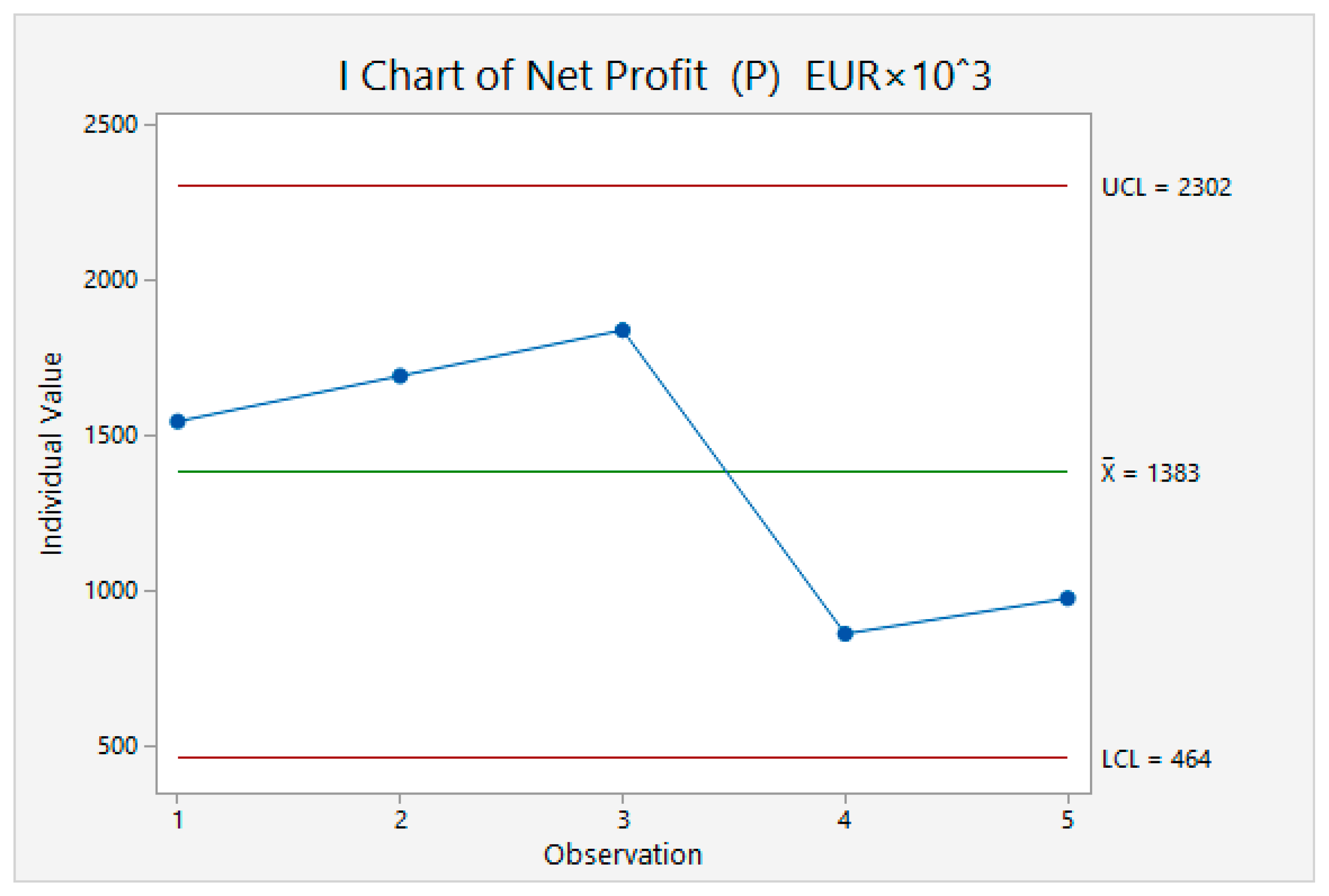
We determined the control diagrams for the three financial variables with which we operate in the design part of the article to verify the usefulness of the proposed solution in comparing the conventional procedure of statistical regulation applied to financial variables. These are revenues of R over time (Figure 3), profits P over time (Figure 4), and net profitability of revenues P/R over time. In these all quantities are stable in the observed time during the reference period. After the third time period, revenues grew, but profits declined. This fact indicates a reduction in efficiency to generate profit through demand. Here, the apparent reason is the high unit cost relative to the average price of the product, thus indicating a total decline in product competitiveness. In the fourth period, the situation was stabilized; thus, it returned to normal relations of financial quantities.

Interestingly, we cannot determine the correct causality between profit and yield by statistical regulation or the analysis of categorical data (it turns out that there is a negative correlation (i.e., causally is wrong)), both according to Pearson (=−0.600) and Spearman (=−0.753). This finding slightly disadvantages the credibility in the statistical regulation of the stability of selected variables of production profitability management. Additionally, it shows the importance of a compliant management approach, combining both statistical and dynamic processes, including the determination of transfer functions and algebraic conditions for the stability of financial regulation. Therefore, we approached dynamic stability control using the time expression of transfer functions.

In the discussion, it is also appropriate to summarize the theoretical, practical, and methodological benefits of the proposed solution.

At the theoretical level, sufficient conditions for the stability of a dynamical system have been formulated if we use Laplace transforms of differential equations supplemented by the proof of the theorem. There is a plan for subsequent research (or, more precisely, a method proposal) to determine the stability conditions of a discrete system that does not have a known parametric distribution of random vector and that is subject to extreme (jump) changes in disturbance and load variables. This situation is typical of some areas of today’s business (for example, the hotel and hospitality industry) due to sudden restrictions due to the fight against the COVID-19 pandemic.

At the practical level, the procedure was demonstrated on a case study of food production, a typical representative of the mass output, characterized by instability caused by the excessive variability of material inputs due to the high variability of animal characteristics. Because the data from the income statement, which is the financial analysis input, is used, this procedure is data-intensive. In addition, because the data of standardized financial quantities are used, this procedure is easily transferable to other industrial areas (e.g., mechanical engineering). Transferability to the field of services is possible only after modifying the attribute of production and research because it is not a matter of mass transformation. It is only necessary to design other transfer functions.

From a methodological point of view, this is an anti-parallel method. We determine the transfer functions of the main components of the business model in the sequence of the statistical estimate of the interval of stability of financial variables, which enable the subsequent regulation and determination of dynamic stability conditions. Subsequently, a control mechanism is created for this in an integral and proportional form, which prevents the emergence of a permanent control deviation. In the last step, we determine the diversification of the action. The whole methodology can be regulated, and the correctness of the settings can be verified by the speed of convergence of the control deviation to its equilibrium value. The way to determine the convergence rate is the area of subsequent methodological research.

7. Conclusions

The former simplification assumed that the primary goal of business is to achieve maximum profit. Even today, the business goal formulated and the general decision-making criterion is often emphasized, especially in a company’s statistical microeconomic models. In the current unstable and coincidentally affected pandemic, it is the subject of critical objections because it is a statistical approach that does not consider the time dimension—it does not distinguish at which point the profit was made. The company’s profit, reported in the accounts, is strongly influenced by the chosen concept of income and expenses, the depreciation method, the creation, and the release of reserves and prepaid expenses. Therefore, the need to use cash flows to evaluate the company and investment options is emphasized. Profit maximization is a fundamental business goal that does not consider the different degrees of risk with which the profit is achieved. It assumes that higher yields are achieved with the same degree of risk. This is currently an unrealistic assumption. The overall result must therefore be assessed in terms of the sustainability of the business. For this purpose, it is necessary to determine the stability conditions of the gain quantity concerning the influence of various environmental disturbances. When determining the conditions of stability and the distribution of the investment portfolio, it is possible to achieve the newly formulated business goal (and thus the company’s financial goal), which is currently based on maximizing the company’s market value over time, both in terms of the amount of profit and the risk associated with achieving that profit. To this end, it is necessary to determine the conditions of stability in achieving profit over time. An unconventional and, at the same time, functional method for this stabilization of the profit variable was presented in the Results section of this article.