Linear and Energy-Stable Method with Enhanced Consistency for the Incompressible Cahn–Hilliard–Navier–Stokes Two-Phase Flow Model

Abstract

The Cahn–Hilliard–Navier–Stokes model is extensively used for simulating two-phase incompressible fluid flows. With the absence of exterior force, this model satisfies the energy dissipation law. The present work focuses on developing a linear, decoupled, and energy dissipation-preserving time-marching scheme for the hydrodynamics coupled Cahn–Hilliard model. An efficient time-dependent auxiliary variable approach is first introduced to design equivalent equations. Based on equivalent forms, a BDF2-type linear scheme is constructed. In each time step, the unique solvability and the energy dissipation law can be analytically estimated. To enhance the energy stability and the consistency, we correct the modified energy by a practical relaxation technique. Using the finite difference method in space, the fully discrete scheme is described, and the numerical solutions can be separately implemented. Numerical results indicate that the proposed scheme has desired accuracy, consistency, and energy stability. Moreover, the flow-coupled phase separation, the falling droplet, and the dripping droplet are well simulated.

1. Introduction

Two-phase fluid flows extensively exist in the natural world. The front-tracking method and volume-of-fluid (VOF) method are two typical approaches to model two-phase fluids. Based on the front-tracking method, Masiri [1] investigated the pairwise interaction of two droplets in simple shear flow. Goodarzi et al. [2] adopted the VOF method to numerically study the binary collision of droplets in a horizontal channel. The Cahn–Hilliard (CH) equation [3] is one of the typical models in phase-field field. It was originally derived by Cahn and Hilliard [4] to describe the spinodal decomposition of binary alloys. The phase-field model not only captures the two-phase interface in an implicit manner but also has smooth and conservative solution. Thanks to these features, the phase-field model has been extensively used in multi-phase fluid simulation [5,6,7,8,9,10], image processing [11], topology optimization [12], and computational biology [13,14], etc. Furthermore, the CH equation satisfies the thermodynamics-consistent energy dissipation law. This energy dissipation property is thermodynamically consistent. To numerically meet this physical property, it is suitable to design energy structure-preserving numerical schemes.

To preserve the energy dissipation property of the CH model, the main difficulty is how to discretize the nonlinear term in time. Both fully explicit and fully implicit treatments cannot satisfy the unconditional energy stability. The convex splitting method (CSM) is one of the popular tools for treating the nonlinear term. Based on CSM, various linear and nonlinear time-marching schemes have been constructed in the past decade, see [15,16,17,18] and reference therein. For the purposes of efficiency, energy stability, and high-order accuracy, the auxiliary variable-type methods [19,20] are popular in recent years.

Two-phase incompressible fluid flows exist widely in natural world, such as droplet formation in micro-fluid device [21,22], liquid sloshing in ship and ocean engineering [23], and fluid instability [24], etc. The Cahn–Hilliard–Navier–Stokes (CHNS) model is practical to describe the interfacial change and fluid motion. For this model, the total energy of the system consists of the free energy for phase-field variable and the kinetic energy for velocity field. The coupling terms related to advection and surface tension lead to some difficulties for designing energy-stable numerical schemes. Recently, some researchers [25,26,27] adopted the original SAV approach to develop linear and energy-stable schemes for the flow-coupled phase-field problems. This idea used an introduced auxiliary variable to cancel the inner products related to coupling terms. Therefore, the energy dissipation property can be easily estimated. However, the original SAV method requires extra computational costs to achieve totally decoupled computation. To fix this drawback, Liu and Li [28] proposed a highly efficient variant of SAV method for generalized dissipative system. In their proposed schemes, all variables were decoupled in time and were updated in a step-by-step manner. Later, Zheng and Li [29] extended this method to Cahn–Hilliard–Brinkman (CHB) model describing two-phase creeping flow. Yang and Kim [30] used the similar method to develop efficient and stable algorithm for the ternary CHNS model. We note that another drawback of auxiliary variable-type methods is the resulting discrete version of energy dissipation law corresponds to a modified energy functional instead of the original one. Therefore, the consistency between original energy and modified energy is hard to theoretically satisfy. To overcome this, Jiang et al. [31] recently developed a simple energy relaxation method to enhance the consistency. By following similar idea, Zhang and Shen [32] constructed a novel relaxation technique for the efficient variants of SAV method. The present auxiliary variable methods with energy relaxation are only applied for phase-field models with the absence of fluid flows. In this work, we aim to develop a new variant with enhanced consistency, energy stability, and efficient algorithm for the CHNS two-phase fluid model.

The main scientific contributions of this work are: (i) all variables are totally decoupled by introducing an appropriate time-dependent auxiliary variable; (ii) the solution algorithm is highly efficient because we only need to solve several linear elliptic equations; (iii) the energy stability with respect to modified energy can be easily proved; (iv) the stability and consistency are improved using a correction technique. To the best of our knowledge, this is the first work focusing on an efficiently linear, energy-stable, and highly consistent time-marching scheme for the incompressible CHNS fluid model.

The rest is organized as follows. In Section 2, the incompressible CHNS model is briefly described. In Section 3, we introduce the equivalent forms and propose the linearly decoupled scheme. The energy stability is estimated, and the fully discrete implementation is given. In Section 4, various numerical simulations are performed to verify the accuracy, stability, and capability. The concluding remarks are drawn in Section 5.

2. Cahn–Hilliard–Navier–Stokes Model

Some notations are introduced here, we denote the $L^2$-inner product of two functions as $(f_1,f_2)={\int }_{\Omega }{f}_1{f}_{2}d\mathbf{x}$, where $f_1=f_1(\mathbf{x})$ and $f_2=f_2(\mathbf{x})$. The $L^2$-norm of $f_1$ is denoted as $\parallel f_1{\parallel }^2=(f_1,f_1)$.

Let $\Omega$ be a computational domain in ${\mathbb{R}}^d$, where d is the dimensional of space. In particular, the rectangular domain is used in two-dimensional space. The domain $\Omega$ is filled with two incompressible and immiscible fluids. The phase-field variable (order parameter) $\varphi =\varphi (\mathbf{x},t)$ is used to represent two fluids. Here, $\mathbf{x}$ and t are spatial and temporal variables. In the bulk of one fluid, we define $\varphi =1$ and let $\varphi =-1$ in another bulk. The phase-field method assumes that a smooth and narrow transition layer exists across the interface between two fluids. The thickness of the transition layer is controlled by a small positive constant $ϵ$. After the non-dimensionalization as in [33], the CHNS model describing two-phase incompressible fluid flow is expressed as

$$\begin{array}{ccc}& & \frac{\partial \mathbf{u}}{\partial t}+\mathbf{u}·\nabla \mathbf{u}=-\nabla p+\frac{1}{Re}\Delta \mathbf{u}-\frac{1}{We}\varphi \nabla \mu ,\hfill \end{array}$$

(1)

$$\begin{array}{ccc}& & \nabla ·\mathbf{u}=0,\hfill \end{array}$$

(2)

$$\begin{array}{ccc}& & \frac{\partial \varphi }{\partial t}+\nabla ·(\mathbf{u}\varphi )=\frac{1}{Pe}\Delta \mu ,\hfill \end{array}$$

(3)

$$\begin{array}{ccc}& & \mu =\lambda (F^{\prime }(\varphi )-{ϵ}^2\Delta \varphi ),\hfill \end{array}$$

(4)

where $\mathbf{u}$ is velocity field. In 2D space, we have $\mathbf{u}=(u,v)$, u and v are velocity components along x- and y-directions. The pressure is p, $\varphi \nabla \mu$ represents the surface tension. Non-dimensional numbers are Reynolds number $Re$, Weber number $We$, and Peclet number $Pe$. The chemical potential is $\mu$, $F(\varphi )=0.25{({\varphi }^2-1)}^2$ is a nonlinear potential which accounts for phase separation, $F^{\prime }(\varphi )={\varphi }^3-\varphi$, $\lambda >0$ is a constant. To obtain the desired energy dissipation property, we consider the periodic boundary condition or the following boundary conditions on $\partial \Omega$

$$\begin{array}{c}\hfill {\nabla \varphi ·\mathbf{n}|}_{\partial \Omega }{=\nabla \mu ·\mathbf{n}|}_{\partial \Omega }=\nabla p·\mathbf{n}{{|}_{\partial \Omega }=\mathbf{u}·\mathbf{n}|}_{\partial \Omega }=0.\end{array}$$

It is worth noting that the periodic condition and the above conditions are used to eliminate the boundary effects in energy estimations. The initial conditions are ${\mathbf{u}|}_{t=0}={\mathbf{u}}^0$, ${p|}_{t=0}=p^0$, and ${\varphi |}_{t=0}={\varphi }^0$.

Theorem 1. 

With the assumptions of existence and enough smoothness of solution ϕ, the mass conservation (i.e., $\frac{d}{dt}{\int }_{\Omega }\varphi d\mathbf{x}=0$) holds.

Proof. 

By taking the $L^2$-inner product of Equation (3) with $\mathbf{1}$, we have

$$\begin{array}{ccc}\hfill \frac{d}{dt}{\int }_{\Omega }\varphi d\mathbf{x}& =& {\int }_{\Omega }\left[\frac{1}{Pe}\Delta \mu -\nabla ·(\mathbf{u}\varphi )\right]d\mathbf{x}\hfill \end{array}$$

(5)

$$\begin{array}{ccc}& =& \frac{1}{Pe}{\int }_{\partial \Omega }\nabla \mu ·\mathbf{n}ds-{\int }_{\partial \Omega }(\mathbf{u}\varphi )·\mathbf{n}ds=0,\hfill \end{array}$$

(6)

where the divergence theorem and appropriate boundary condition are used. The proof is completed.    □

Theorem 2. 

The CHNS model satisfies the energy dissipation law with respect to the following total energy

$$\begin{array}{c}\hfill E(\mathbf{u},\varphi )={\int }_{\Omega }\left[\frac{We}{2}{|\mathbf{u}|}^2+\lambda \left(\frac{{ϵ}^2}{2}{|\nabla \varphi |}^2+F(\varphi )\right)\right]d\mathbf{x},\end{array}$$

(7)

Proof. 

By taking the $L^2$-inner product of Equation (1) with $We\mathbf{u}$, we have

$$\begin{array}{c}\hfill \frac{d}{dt}{\int }_{\Omega }\frac{We}{2}{|\mathbf{u}|}^{2}d\mathbf{x}=-\frac{We}{Re}{\parallel \nabla \mathbf{u}\parallel }^2-(\varphi \nabla \mu ,\mathbf{u}),\end{array}$$

(8)

where $(\mathbf{u}·\nabla \mathbf{u},\mathbf{u})=0$ and $(\nabla p,\mathbf{u})=0$ are used. Based on appropriate boundary conditions of $\mathbf{u}$ and p, these two equalities have been analytically proved in previous works, see [34,35] for some details.

By taking the $L^2$-inner product of Equation (3) with $\mu$, of Equation (4) with $\frac{\partial \varphi }{\partial t}$, we have

$$\begin{array}{ccc}& & \left(\frac{\partial \varphi }{\partial t},\mu \right)+(\nabla ·(\mathbf{u}\varphi ),\mu )=-\frac{1}{Pe}{\parallel \nabla \mu \parallel }^2.\hfill \end{array}$$

(9)

$$\begin{array}{ccc}& & \left(\mu ,\frac{\partial \varphi }{\partial t}\right)=\frac{d}{dt}{\int }_{\Omega }\lambda \left(\frac{{ϵ}^2}{2}{|\nabla \varphi |}^2+F(\varphi )\right)d\mathbf{x}.\hfill \end{array}$$

(10)

By combining Equations (8)–(10), we derive

$$\begin{array}{c}\hfill \frac{d}{dt}E(\mathbf{u},\varphi )=-\frac{We}{Re}{\parallel \nabla \mathbf{u}\parallel }^2-\frac{1}{Pe}{\parallel \nabla \mu \parallel }^2\le 0,\end{array}$$

(11)

where $(\nabla ·(\mathbf{u}\varphi ),\mu )+(\varphi \nabla \mu ,\mathbf{u})=0$ is used. Based on appropriate boundary conditions, Zhu et al. [35] proved this equality in detail. The proof is completed.    □

3. Numerical Scheme, Analysis, and Implementation

3.1. Time-Marching Scheme for the CHNS Model

In this work, we aim to develop a linearly decoupled, second-order time-accurate, and unconditionally energy-stable method for the CHNS system. However, the desired properties (i.e., linearly decoupled computation, second-order accuracy, and energy law) are hard to satisfy if we directly design time-marching scheme for Equations (1)–(4). To overcome this difficulty, a natural approach is to transform the original equations into equivalent forms by introducing appropriate auxiliary variables. Herein, the time-dependent auxiliary variables are defined as $R=E(\mathbf{u},\varphi )$ and $q=R/E(\mathbf{u},\varphi )$, we rewrite Equations (1)–(4) to be

$$\begin{array}{ccc}& & \frac{\partial \mathbf{u}}{\partial t}+Q\mathbf{u}·\nabla \mathbf{u}=-\nabla p+\frac{1}{Re}\Delta \mathbf{u}-\frac{Q}{We}\varphi \nabla \mu ,\hfill \end{array}$$

(12)

$$\begin{array}{ccc}& & \nabla ·\mathbf{u}=0,\hfill \end{array}$$

(13)

$$\begin{array}{ccc}& & \frac{\partial \varphi }{\partial t}+Q\nabla ·(\mathbf{u}\varphi )=\frac{1}{Pe}\Delta \mu ,\hfill \end{array}$$

(14)

$$\begin{array}{ccc}& & \mu =\lambda (Q{F}^{\prime }(\varphi )-{ϵ}^2\Delta \varphi ),\hfill \end{array}$$

(15)

$$\begin{array}{ccc}& & q=\frac{R}{E(\mathbf{u},\varphi )},Q=q(2-q)\hfill \end{array}$$

(16)

$$\begin{array}{ccc}& & \frac{dR}{dt}=-\frac{R}{E(\mathbf{u},\varphi )}\left(\frac{We}{Re}{\parallel \nabla \mathbf{u}\parallel }^2+\frac{1}{Pe}{\parallel \nabla \mu \parallel }^2\right).\hfill \end{array}$$

(17)

From the definition of R, we observe that $q=\frac{R}{E(\mathbf{u},\varphi )}=1$. Because $Q=q(2-q)$, it is obvious that $Q=1$. Therefore, Equations (12)–(15) and Equations (1)–(4) are equivalent. For the introduced variable R, Equation (17) provides its evolutional equation. Since R is an equivalent form of total energy, the right-hand side of Equation (17) is derived from (11). Let T and $N^T$ be the total computational time and the number of time iteration, respectively. The uniform time step is defined as $\Delta t=T/N^T$. The proposed temporally second-order accurate scheme based on second-order backward difference formula (BDF2) consists of two steps.

Step 1. Let ${(·)}^{n+1}$ be a variable at $(n+1)$-th time level. With the computed variables at n-th and $(n-1)$-th time levels, we update ${\tilde{\mathbf{u}}}^{n+1}$, $p^{n+1}$, ${\mathbf{u}}^{n+1}$, ${\varphi }^{n+1}$, and ${\tilde{R}}^{n+1}$ by

$$\begin{array}{ccc}& & \frac{3{\tilde{\mathbf{u}}}^{n+1}-4{\mathbf{u}}^n+{\mathbf{u}}^{n-1}}{2\Delta t}+Q^{n+1}{\mathbf{u}}^{*}·\nabla {\mathbf{u}}^{*}=-\nabla p^n+\frac{1}{Re}\Delta {\tilde{\mathbf{u}}}^{n+1}-\frac{Q^{n+1}}{We}{\varphi }^{*}\nabla {\mu }^{*},\hfill \end{array}$$

(18)

$$\begin{array}{ccc}& & \frac{3{\mathbf{u}}^{n+1}-3{\tilde{\mathbf{u}}}^{n+1}}{2\Delta t}=-\nabla (p^{n+1}-p^n),\hfill \end{array}$$

(19)

$$\begin{array}{ccc}& & \nabla ·{\mathbf{u}}^{n+1}=0,\hfill \end{array}$$

(20)

$$\begin{array}{ccc}& & \frac{3{\varphi }^{n+1}-4{\varphi }^n+{\varphi }^{n-1}}{2\Delta t}+Q^{n+1}\nabla ·({\mathbf{u}}^{*}{\varphi }^{*})=\frac{1}{Pe}\Delta {\mu }^{n+1},\hfill \end{array}$$

(21)

$$\begin{array}{ccc}& & {\mu }^{n+1}=\lambda \left(Q^{n+1}{F}^{\prime }({\varphi }^{*})-{ϵ}^2\Delta {\varphi }^{n+1}+S({\varphi }^{n+1}-{\varphi }^{*})\right),\hfill \end{array}$$

(22)

$$\begin{array}{ccc}& & q^{n+1}=\frac{{\tilde{R}}^{n+1}}{E({\mathbf{u}}^{*},{\varphi }^{*})},Q^{n+1}=q^{n+1}(2-q^{n+1}),\hfill \end{array}$$

(23)

$$\begin{array}{ccc}& & \frac{{\tilde{R}}^{n+1}-R^n}{\Delta t}=-\frac{{\tilde{R}}^{n+1}}{E({\mathbf{u}}^{*},{\varphi }^{*})}\left(\frac{We}{Re}\parallel \nabla {\mathbf{u}}^{*}{\parallel }^2+\frac{1}{Pe}{\parallel \nabla {\mu }^{*}\parallel }^2\right).\hfill \end{array}$$

(24)

Here, ${(·)}^{*}=2{(·)}^n-{(·)}^{n-1}$ is the explicit extrapolation, ${\tilde{\mathbf{u}}}^{n+1}$ is the intermediate velocity field. On $\partial \Omega$, we consider the periodic or the following boundary conditions

$$\begin{array}{c}\hfill {\mathbf{u}}^{n+1}{·\mathbf{n}|}_{\partial \Omega }=0,{\tilde{\mathbf{u}}}^{n+1}{|}_{\partial \Omega }=0,\nabla {\varphi }^{n+1}{·\mathbf{n}|}_{\partial \Omega }=\nabla {\mu }^{n+1}{·\mathbf{n}|}_{\partial \Omega }=0,\nabla p^{n+1}·\mathbf{n}{{|}_{\partial \Omega }=\nabla p^n·\mathbf{n}|}_{\partial \Omega }.\end{array}$$

Note Equation (24) is a temporally first-order accurate scheme, which means $q^{n+1}$ is a first-order approximation to 1. From the definition of $Q^{n+1}$ in Equation (23), we observe $Q^{n+1}$ is a second-order approximation to 1. Therefore, the second-order accuracy of Equations (18)–(22) is still satisfied. Although $R=E(\mathbf{u},\varphi )$ holds in continuous version, the discrete value of ${\tilde{R}}^n$ is not equal to the discrete version of original energy (i.e., $E({\mathbf{u}}^n,{\varphi }^n)$). Although the energy stability of the above scheme can be estimated by following the similar procedure as in [30], the resulting modified energy and its original version are not consistent. The inconsistent energy will destroy the desired energy stability. To enhance the consistency, we next perform the correction step as follows.

Step 2. Inspired by [31,32], we correct the energy to be

$$\begin{array}{c}\hfill R^{n+1}={\xi }_0{\tilde{R}}^{n+1}+(1-{\xi }_0)E({\mathbf{u}}^{n+1},{\varphi }^{n+1}),{\xi }_0\in \mathcal{I},\end{array}$$

(25)

where $R^{n+1}$ is the corrected energy, ${\tilde{R}}^{n+1}$ is a modified energy, and $E({\mathbf{u}}^{n+1},{\varphi }^{n+1})$ is the discrete original energy. Here,

$$\begin{array}{c}\hfill \mathcal{I}=\left\{\xi \in [0,1]s.t.\frac{R^{n+1}-{\tilde{R}}^{n+1}}{\Delta t}\le -{\theta }^{n+1}\left(\frac{1}{Pe}\parallel \nabla {\mu }^{n+1}{\parallel }^2+\frac{We}{Re}{\parallel \nabla {\mathbf{u}}^{n+1}\parallel }^2\right)\right.\\ \hfill \left.+\frac{{\tilde{R}}^{n+1}}{E({\mathbf{u}}^{*},{\varphi }^{*})}\left(\frac{1}{Pe}\parallel \nabla {\mu }^{*}{\parallel }^2+\frac{We}{Re}{\parallel \nabla {\mathbf{u}}^{*}\parallel }^2\right)\right\}.\end{array}$$

(26)

Here, ${\theta }^{n+1}\ge 0$ and $\mathcal{I}$ is not empty because $\xi =1$ is in $\mathcal{I}$. It is worth noting that the inequality in Equation (26) is used to choose an appropriate value of $\xi$ such that the corrected energy $R^{n+1}$ strictly satisfies the energy dissipation law. Please refer to the proof of Theorem 4 for some details. By substituting $R^{n+1}$ in Equation (26) by Equation (25), we obtain

$$\begin{array}{ccc}\hfill ({\tilde{R}}^{n+1}-E({\mathbf{u}}^{n+1},{\varphi }^{n+1})){\xi }_0& \le & {\tilde{R}}^{n+1}-E({\mathbf{u}}^{n+1},{\varphi }^{n+1})-\Delta t{\theta }^{n+1}\left(\frac{1}{Pe}\parallel \nabla {\mu }^{n+1}{\parallel }^2+\frac{We}{Re}{\parallel \nabla {\mathbf{u}}^{n+1}\parallel }^2\right)\hfill \\ & & +\frac{\Delta t{\tilde{R}}^{n+1}}{E({\mathbf{u}}^{*},{\varphi }^{*})}\left(\frac{1}{Pe}\parallel \nabla {\mu }^{*}{\parallel }^2+\frac{We}{Re}{\parallel \nabla {\mathbf{u}}^{*}\parallel }^2\right).\hfill \end{array}$$

(27)

The possible choices of ${\xi }_0$ and ${\theta }^{n+1}$ are as follows:

(i)

If ${\tilde{R}}^{n+1}=E({\mathbf{u}}^{n+1},{\varphi }^{n+1})$, we let ${\xi }_0=0$ and ${\theta }^{n+1}=\frac{{\tilde{R}}^{n+1}(\frac{1}{Pe}\parallel \nabla {\mu }^{*}{\parallel }^2+\frac{We}{Re}\parallel \nabla {\mathbf{u}}^{*}{\parallel }^2)}{E({\mathbf{u}}^{*},{\varphi }^{*})(\frac{1}{Pe}\parallel \nabla {\mu }^{n+1}{\parallel }^2+\frac{We}{Re}\parallel \nabla {\mathbf{u}}^{n+1}{\parallel }^2)}$,

(ii)

If ${\tilde{R}}^{n+1}>E({\mathbf{u}}^{n+1},{\varphi }^{n+1})$, we let ${\xi }_0=0$ and

$$\begin{array}{c}\hfill {\theta }^{n+1}=\frac{{\tilde{R}}^{n+1}-E({\mathbf{u}}^{n+1},{\varphi }^{n+1})}{\Delta t(\frac{1}{Pe}\parallel \nabla {\mu }^{n+1}{\parallel }^2+\frac{We}{Re}\parallel \nabla {\mathbf{u}}^{n+1}{\parallel }^2)}+\frac{{\tilde{R}}^{n+1}(\frac{1}{Pe}\parallel \nabla {\mu }^{*}{\parallel }^2+\frac{We}{Re}\parallel \nabla {\mathbf{u}}^{*}{\parallel }^2)}{E({\mathbf{u}}^{*},{\varphi }^{*})(\frac{1}{Pe}\parallel \nabla {\mu }^{n+1}{\parallel }^2+\frac{We}{Re}\parallel \nabla {\mathbf{u}}^{n+1}{\parallel }^2)},\end{array}$$

(iii)

If ${\tilde{R}}^{n+1}<E({\mathbf{u}}^{n+1},{\varphi }^{n+1})$ and

$$\begin{array}{c}\hfill {\tilde{R}}^{n+1}-E({\mathbf{u}}^{n+1},{\varphi }^{n+1})+\frac{\Delta t{\tilde{R}}^{n+1}}{E({\mathbf{u}}^{*},{\varphi }^{*})}\left(\frac{1}{Pe}\parallel \nabla {\mu }^{*}{\parallel }^2+\frac{We}{Re}{\parallel \nabla {\mathbf{u}}^{*}\parallel }^2\right)\ge 0,\end{array}$$

we let ${\xi }_0=0$ and ${\theta }^{n+1}$ take the same value in (ii).

(iv)

If ${\tilde{R}}^{n+1}<E({\mathbf{u}}^{n+1},{\varphi }^{n+1})$ and

$$\begin{array}{c}\hfill {\tilde{R}}^{n+1}-E({\mathbf{u}}^{n+1},{\varphi }^{n+1})+\frac{\Delta t{\tilde{R}}^{n+1}}{E({\mathbf{u}}^{*},{\varphi }^{*})}\left(\frac{1}{Pe}\parallel \nabla {\mu }^{*}{\parallel }^2+\frac{We}{Re}{\parallel \nabla {\mathbf{u}}^{*}\parallel }^2\right)<0,\end{array}$$

we let ${\theta }^{n+1}=0$ and

$$\begin{array}{c}\hfill {\xi }_0=1-\frac{\Delta t{\tilde{R}}^{n+1}(\frac{1}{Pe}\parallel \nabla {\mu }^{*}{\parallel }^2+\frac{We}{Re}\parallel \nabla {\mathbf{u}}^{*}{\parallel }^2)}{E({\mathbf{u}}^{*},{\varphi }^{*})(E({\mathbf{u}}^{n+1},{\varphi }^{n+1})-{\tilde{R}}^{n+1})}.\end{array}$$

Theorem 3. 

Equations (18)–(24) admit unique solutions: ${\varphi }^{n+1}$, ${\mathbf{u}}^{n+1}$, and $p^{n+1}$.

Proof. 

From Equation (24), we obtain

$$\begin{array}{c}\hfill {\tilde{R}}^{n+1}=R^n/\left[1+\frac{\Delta t}{E({\mathbf{u}}^{*},{\varphi }^{*})}\left(\frac{We}{Re}\parallel \nabla {\mathbf{u}}^{*}{\parallel }^2+\frac{1}{Pe}{\parallel \nabla {\mu }^{*}\parallel }^2\right)\right].\end{array}$$

(28)

It is obvious that $E({\mathbf{u}}^{*},{\varphi }^{*})\ge 0$, thus the denominator in Equation (28) is larger than zero, ${\tilde{R}}^{n+1}$ can be directly updated. Next, we estimate the unique solvability for ${\varphi }^{n+1}$. By combining Equations (21) and (22), we have

$$\begin{array}{ccc}\hfill \frac{3{\varphi }^{n+1}-4{\varphi }^n+{\varphi }^{n-1}}{2\Delta t}+Q^{n+1}\nabla ·({\mathbf{u}}^{*}{\varphi }^{*})& =& \frac{\lambda }{Pe}\Delta \left[Q^{n+1}{F}^{\prime }({\varphi }^{*})-{ϵ}^2\Delta {\varphi }^{n+1}+S({\varphi }^{n+1}-{\varphi }^{*})\right].\hfill \end{array}$$

(29)

A convex functional is defined as

$$\begin{array}{c}\hfill \mathcal{F}(\varphi )={\int }_{\Omega }\left[\frac{3}{4\Delta t}{|\varphi |}^2+\frac{S\lambda }{2Pe}{|\nabla \varphi |}^2+\frac{{ϵ}^2\lambda }{2Pe}{|\Delta \varphi |}^2+s^{n,n-1}\psi \right]d\mathbf{x},\end{array}$$

(30)

where

$$\begin{array}{c}\hfill s^{n,n-1}=\frac{-4{\varphi }^n+{\varphi }^{n-1}}{2\Delta t}+\frac{\lambda Q^{n+1}}{Pe}\Delta F^{\prime }({\varphi }^{*})-\frac{S\lambda }{Pe}\Delta {\varphi }^{*}+Q^{n+1}\nabla ·({\mathbf{u}}^{*}{\varphi }^{*}).\end{array}$$

By taking the variational approach for $\mathcal{F}(\varphi )$ at $(n+1)$-th time level, we obtain

$$\begin{array}{c}\hfill \frac{\delta \mathcal{F}}{\delta \varphi }{|}_{\varphi ={\varphi }^{n+1}}=\frac{3}{2\Delta t}{\varphi }^{n+1}-\frac{S\lambda }{Pe}\Delta {\varphi }^{n+1}+\frac{{ϵ}^2\lambda }{Pe}{\Delta }^2{\varphi }^{n+1}+s^{n,n-1}.\end{array}$$

(31)

For a convex functional, its unique minimum value exists as $\delta \mathcal{F}/\delta \varphi =0$. In this sense, the minimization of $\mathcal{F}({\varphi }^{n+1})$ and the solution of Equation (29) are equivalent. We complete the estimation of unique solvability for ${\varphi }^{n+1}$. The unique solvability for ${\mathbf{u}}^{n+1}$ can be estimated in a similar manner. To keep the presentation short, we omit these steps and interested readers can refer to [30] for some details.    □

Theorem 4. 

The solutions of Equations (18)–(24) and Equation (25) dissipate a modified energy ${\tilde{R}}^n$ and a corrected energy $R^n$. Furthermore, ${\tilde{R}}^n$ and $R^n$ satisfy the bounded-from-below condition.

Proof. 

With an initial value $R^0\ge 0$, we know ${\tilde{R}}^1\ge 0$ from Equation (28). Based on the facts: ${\xi }_0\in [0,1]$ and $E({\mathbf{u}}^1,{\varphi }^1)\ge 0$, we can obtain $R^1\ge 0$ from Equation (25). By the induction, we easily derive $R^n>0$. From Equation (24), we have

$$\begin{array}{c}\hfill \frac{{\tilde{R}}^{n+1}-R^n}{\Delta t}=-\frac{{\tilde{R}}^{n+1}}{E({\mathbf{u}}^{*},{\varphi }^{*})}\left(\frac{We}{Re}\parallel \nabla {\mathbf{u}}^{*}{\parallel }^2+\frac{1}{Pe}{\parallel \nabla {\mu }^{*}\parallel }^2\right)\le 0,\end{array}$$

(32)

where ${\tilde{R}}^{n+1}\ge 0$ and $E({\mathbf{u}}^{*},{\varphi }^{*})\ge 0$ are used. The above inequality indicates the modified energy law, i.e., ${\tilde{R}}^{n+1}\le R^n$. By combining (24) and (26), we have

$$\begin{array}{c}\hfill \frac{R^{n+1}-R^n}{\Delta t}=-{\theta }^{n+1}\left(\frac{1}{Pe}\parallel \nabla {\mu }^{n+1}{\parallel }^2+\frac{We}{Re}{\parallel \nabla {\mathbf{u}}^{n+1}\parallel }^2\right)\le 0,\end{array}$$

(33)

which indicates the corrected energy law, i.e., $R^{n+1}\le R^n$. Based on ${\xi }_0\in [0,1]$, ${\tilde{R}}^{n+1}\ge 0$, and Equation (25), we derive $R^{n+1}\ge 0$. We complete the estimation.    □

In each time step, the calculations are summarized as follows:

• Calculate ${\tilde{R}}^{n+1}$ from Equation (24);
• Calculate $q^{n+1}$ and $Q^{n+1}$ from Equation (23);
• Update ${\varphi }^{n+1}$ by solving Equations (21) and (22);
• Update ${\mathbf{u}}^{n+1}$ and $p^{n+1}$ from Equations (18)–(20);
• Update $R^{n+1}$ from Equation (25).

3.2. Fully Discrete Implementation

We discretize the space using marker-and-cell (MAC) finite difference method (FDM) [36,37] in which $\varphi$ and p locate at cell centers, the velocity components locate at cell edges. Let the domain be $\Omega =(0,L_x)\times (0,L_y)$. The uniform mesh size is $h=L_x/N_x=L_y/N_y$, where $N_x$ and $N_y$ are positive even integers. Let ${\varphi }_{ij}^n$, ${\mu }_{ij}^n$, and $p_{ij}^n$ be approximations of $\varphi (x_i,y_j,n\Delta t)$, $\mu (x_i,y_j,n\Delta t)$, and $p(x_i,y_j,n\Delta t)$, respectively. The spatial points are $x_i=\left(i-\frac{1}{2}\right)h$, $y_j=\left(j-\frac{1}{2}\right)h$, $i=1,2,\cdots ,N_x$, and $j=1,2,\cdots ,N_y$. Let $u_{i+\frac{1}{2},j}^n$ and $v_{i,j+\frac{1}{2}}^n$ be the approximations of $u(x_{i+\frac{1}{2}},y_j,n\Delta t)$ and $v(x_i,y_{j+\frac{1}{2}},n\Delta t)$, respectively.

At first, ${\tilde{R}}^{n+1}$ is updated by

$$\begin{array}{c}\hfill \frac{{\tilde{R}}^{n+1}-R^n}{\Delta t}=-\frac{{\tilde{R}}^{n+1}}{E^d({\mathbf{u}}^{*},{\varphi }^{*})}\left(\frac{We}{Re}\parallel {\nabla }_d{\mathbf{u}}^{*}{\parallel }_d^2+\frac{1}{Pe}{\parallel \nabla {\mu }^{*}\parallel }_d^2\right).\end{array}$$

(34)

The fully discrete version of total energy is

$$\begin{array}{ccc}\hfill E^d({\mathbf{u}}^n,{\varphi }^n)& =& \frac{We{h}^2}{2}\left(\sum _{i=0}^{N_x}\sum _{j=1}^{N_y}|u_{i+\frac{1}{2},j}^n{|}^2+\sum _{i=1}^{N_x}\sum _{j=0}^{N_y}{|v_{i,j+\frac{1}{2}}^n|}^2\right)\hfill \\ & +& \frac{{ϵ}^2\lambda h^2}{2}\left(\sum _{i=0}^{N_x}\sum _{j=1}^{N_y}|D_x{\varphi }_{i+\frac{1}{2},j}^n{|}^2+\sum _{i=1}^{N_x}\sum _{j=0}^{N_y}{|D_y{\varphi }_{i,j+\frac{1}{2}}^n|}^2\right)+\lambda h^2\sum _{i=1}^{N_x}\sum _{j=1}^{N_y}F({\varphi }_{ij}^n),\hfill \end{array}$$

(35)

where

$$\begin{array}{c}\hfill D_x{\varphi }_{i+\frac{1}{2},j}^n=\frac{{\varphi }_{i+1,j}^n-{\varphi }_{ij}^n}{h},D_y{\varphi }_{i,j+\frac{1}{2}}^n=\frac{{\varphi }_{i,j+1}^n-{\varphi }_{ij}^n}{h}.\end{array}$$

The discrete norms in Equation (34) are

$$\begin{array}{c}\hfill \parallel {\nabla }_d{\mathbf{u}}^{*}{\parallel }_d^2={\nabla }_d{\mathbf{u}}^{*}:{\nabla }_d{\mathbf{u}}^{*},{\parallel \nabla {\mu }^{*}\parallel }_d^2=h^2\left(\sum _{i=0}^{N_x}\sum _{j=1}^{N_y}|D_x{\mu }_{i+\frac{1}{2},j}^{*}{|}^2+\sum _{i=1}^{N_x}\sum _{j=0}^{N_y}{|D_y{\mu }_{i,j+\frac{1}{2}}^{*}|}^2\right),\end{array}$$

where: is the double dot product in tensor operation. Next, we update ${\varphi }_{ij}^{n+1}$ from the following fully discrete system

$$\begin{array}{ccc}& & \frac{3{\varphi }_{ij}^{n+1}-4{\varphi }_{ij}^n+{\varphi }_{ij}^{n-1}}{2\Delta t}+Q^{n+1}{\nabla }_d·{({\mathbf{u}}^{*}{\psi }^{*})}_{ij}=\frac{1}{Pe}\Delta {\mu }_{ij}^{n+1},\hfill \end{array}$$

(36)

$$\begin{array}{ccc}& & {\mu }_{ij}^{n+1}=\lambda \left(Q^{n+1}{F}^{\prime }({\varphi }_{ij}^{*})-{ϵ}^2{\Delta }_d{\varphi }_{ij}^{n+1}+S({\varphi }_{ij}^{n+1}-{\varphi }_{ij}^{*})\right),\hfill \end{array}$$

(37)

where the discrete versions of divergence and Laplacian operators are

$$\begin{array}{ccc}\hfill {\nabla }_d·{(\mathbf{u}\varphi )}_{ij}& =& \frac{u_{i+\frac{1}{2},j}({\varphi }_{i+1,j}+{\varphi }_{ij})-u_{i-\frac{1}{2},j}({\varphi }_{ij}+{\varphi }_{i-1,j})}{2h}\hfill \\ & & +\frac{v_{i,j+\frac{1}{2}}({\varphi }_{i,j+1}+{\varphi }_{ij})-v_{i,j-\frac{1}{2}}({\varphi }_{ij}+{\varphi }_{i,j-1})}{2h},\hfill \\ \hfill {\Delta }_d{\varphi }_{ij}& =& \frac{{\varphi }_{i+1,j}+{\varphi }_{i-1,j}+{\varphi }_{i,j+1}+{\varphi }_{i,j-1}-4{\varphi }_{ij}}{h^2}.\hfill \end{array}$$

The discrete velocity components are updated from the following fully discrete momentum equations

$$\begin{array}{cc}\hfill \frac{3{\tilde{u}}_{i+\frac{1}{2},j}^{n+1}-4u_{i+\frac{1}{2},j}^n+u_{i+\frac{1}{2},j}^{n-1}}{2\Delta t}+Q^{n+1}{(u{u}_x+v{u}_y)}_{i+\frac{1}{2},j}^{*}& =-\frac{p_{i+1,j}^n-p_{ij}^n}{h}+\frac{1}{Re}{\Delta }_d{\tilde{u}}_{i+\frac{1}{2},j}^{n+1}\hfill \\ & -\frac{Q^{n+1}}{2hWe}({\varphi }_{i+1,j}^{*}+{\varphi }_{ij}^{*})({\mu }_{i+1,j}^{*}-{\mu }_{ij}^{*}),\hfill \end{array}$$

(38)

$$\begin{array}{cc}\hfill \frac{3{\tilde{v}}_{i,j+\frac{1}{2}}^{n+1}-4v_{i,j+\frac{1}{2}}^n+v_{i,j+\frac{1}{2}}^{n-1}}{2\Delta t}+Q^{n+1}{(u{v}_x+v{v}_y)}_{i,j+\frac{1}{2}}^{*}& =-\frac{p_{i,j+1}^n-p_{ij}^n}{h}+\frac{1}{Re}{\Delta }_d{\tilde{v}}_{i,j+\frac{1}{2}}^{n+1}\hfill \\ & -\frac{Q^{n+1}}{2hWe}({\varphi }_{i,j+1}^{*}+{\varphi }_{ij}^{*})({\mu }_{i,j+1}^{*}-{\mu }_{ij}^{*}).\hfill \end{array}$$

(39)

The central difference [38,39] is effective to construct energy-stable discretizations for ${(u{u}_x+v{u}_y)}_{i+\frac{1}{2},j}^{*}$ and ${(u{v}_x+v{v}_y)}_{i,j+\frac{1}{2}}^{*}$. To avoid oscillation, the second-order ENO scheme [40] will be a good choice. By taking the discrete divergence operation to Equation (19) and using the discrete divergence-free condition, $p_{ij}^{n+1}$ is updated by solving

$$\begin{array}{ccc}\hfill \frac{p_{i+1,j}^{n+1}+p_{i-1,j}^{n+1}+p_{i,j+1}^{n+1}+p_{i,j-1}^{n+1}-4p_{ij}^{n+1}}{h^2}& =& \frac{p_{i+1,j}^n+p_{i-1,j}^n+p_{i,j+1}^n+p_{i,j-1}^n-4p_{ij}^n}{h^2}\hfill \\ & +& \frac{3}{2\Delta t}\left(\frac{{\tilde{u}}_{i+\frac{1}{2},j}^{n+1}-{\tilde{u}}_{i-\frac{1}{2},j}^{n+1}}{h}+\frac{{\tilde{v}}_{i,j+\frac{1}{2}}-{\tilde{v}}_{i,j-\frac{1}{2}}}{h}\right).\hfill \end{array}$$

(40)

To accelerate the convergence, we herein adopt the linear multigrid algorithm [41].

Remark 1. 

In phase-field model, the thickness of two-phase diffuse interface is controlled by a small positive constant ϵ. Since the governing equations are discretized on spatial grids with uniform mesh size h, Choi et al. [42] presented the following relation to link ϵ and mesh size

$$\begin{array}{c}\hfill ϵ={ϵ}_m=\frac{hm}{2\sqrt{2}{tanh}^{-1}(0.9)}.\end{array}$$

(41)

The above equality indicates that the diffuse interface approximately occupies m grids. The choice of ϵ in the next section follows this formulation.

4. Numerical Simulations

In this section, we first perform some experiments to confirm the temporal accuracy, energy stability, and consistency. To verify the capability, the simulations of flow-coupled phase separation, falling droplet, and liquid jet are conducted. Along x-direction, the periodic boundary condition is used. Along y-direction, we set homogeneous Neumann boundary condition for $\varphi$ and no-slip boundary condition for velocity field.

4.1. Accuracy in Time

In the previous section, the BDF2-type linear discretization was used to construct temporal scheme and the desired accuracy is second-order. To confirm this, we perform the convergence tests to show the accuracy for phase-field variable $\varphi$, velocities u and v, and auxiliary variable Q. In the domain $\Omega =(0,2)\times (0,2)$, the following initial conditions are used

$$\begin{array}{cc}\hfill \varphi (x,y,0)& =tanh\left(\frac{0.3-\sqrt{{(x-1)}^2+{(y-0.7)}^2}}{\sqrt{2}ϵ}\right)\hfill \\ & +tanh\left(\frac{0.3-\sqrt{{(x-1)}^2+{(y-1.3)}^2}}{\sqrt{2}ϵ}\right)+1,\hfill \end{array}$$

(42)

$$\begin{array}{ccc}\hfill u(x,y,0)& =& 0,v(x,y,0)=0,p(x,y,0)=0,Q(0)=1.\hfill \end{array}$$

(43)

To obtain the reference solutions, we use a finer time step $\delta t=0.005h^2$, where $h=1/128$ is the mesh size. The simulations are performed until $t=1.56\times {10}^{-4}$ with different time steps: $\Delta t=2\delta t$, $4\delta t$, $8\delta t$, $16\delta t$, and $32\delta t$. The $L^2$-error is calculated from the difference between the reference and numerical solutions. The parameters are set to be: $ϵ=0.0075$, $\lambda =0.01$, $Pe=1$, $Re=1$, $S=2$, $We=1$. Figure 1a–c plot the errors for $\varphi$, velocities, and Q, respectively. The results indicate that the proposed scheme has second-order accuracy in time.

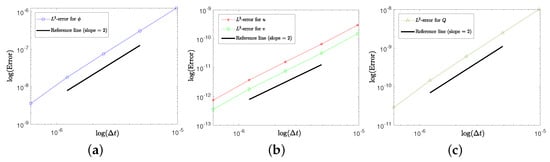
Figure 1. $L^2$-errors for $\varphi$ (a), velocities (b), and Q (c) under different time steps. Here, the log-log view is displayed.

4.2. Energy Stability

The property of energy stability indicates that the total energy of fluid system dissipates in time even if a relatively large time step is used. In discrete version, the correction technique adopted in the previous section is helpful to enhance the stability and consistency. To confirm the desired energy dissipation property and consistency, we consider the evolutions of two adjacent droplets in $\Omega =(0,2)\times (0,2)$. The initial conditions are defined as

$$\begin{array}{cc}\hfill \varphi (x,y,0)& =tanh\left(\frac{0.28-\sqrt{{(x-0.7)}^2+{(y-1)}^2}}{\sqrt{2}ϵ}\right)\hfill \\ & +tanh\left(\frac{0.28-\sqrt{{(x-1.3)}^2+{(y-1)}^2}}{\sqrt{2}ϵ}\right)+1,\hfill \end{array}$$

(44)

$$\begin{array}{ccc}\hfill u(x,y,0)& =& 0,v(x,y,0)=0,p(x,y,0)=0,Q(0)=1.\hfill \end{array}$$

(45)

The parameters are set to be: $h=1/64$, $ϵ=0.015$, $\lambda =0.01$, $Pe=Re=We=1$, and $S=2$. Figure 2a plots the evolutions of corrected energy $R^n$ under different time steps. As we can see, the energy curves are non-increasing in time. In (b), we plot the original energy $E({\mathbf{u}}^n,{\varphi }^n)$ and modified energy ${\tilde{R}}^n$ with a relatively large time step: $\Delta t=0.25$ and without correction technique. We find that the modified energy does not satisfy the dissipative property. In (c), the original energy, modified energy, and corrected energy with correction technique and time step: $\Delta t=0.25$ are plotted. The results indicate that three energy curves are monotonically non-increasing in time. The original energy and corrected energy are highly consistent. The top and bottom rows of Figure 3 display the snapshots of $\varphi$ and velocity field with $\Delta t=0.01$. Under the driven force from surface tension, the initially adjacent droplets merge with each other to form a bigger one.

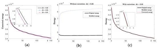
Figure 2. Evolutions of corrected energy under different time steps are shown in (a). With $\Delta t=0.25$, the energy curves without and with correction are plotted in (b,c), respectively.

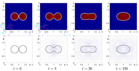
Figure 3. Snapshots of $\varphi$ and velocity field are shown in the top and bottom rows. The computational moments are illustrated under each figure.

4.3. Flow-Coupled Phase Separation

When we consider a homogeneous distribution of $\varphi$ with small perturbation at initial stage, the growth of concentration leads to the formation of two-phase state. This phenomenon is known as phase separation (spinodal decomposition). Phase separation is a basic dynamics of flow-coupled CH system and the pattern formation will be affected by average concentration. In this subsection, we first simulate phase separation with different average concentrations: $\overline{\varphi }=0$ and $0.3$. The domain is $\Omega =(0,2)\times (0,2)$. The initial conditions are defined to be

$$\begin{array}{ccc}\hfill \varphi (x,y,0)& =& \overline{\varphi }+0.001\mathrm{rand}(x,y),\hfill \end{array}$$

(46)

$$\begin{array}{ccc}\hfill u(x,y,0)& =& 0,v(x,y,0)=0,p(x,y,0)=0,Q(0)=1,\hfill \end{array}$$

(47)

where the random value between $-1$ and 1 is denoted by rand$(x,y)$. The parameters are: $\Delta t=0.01$, $h=1/128$, $ϵ=0.0094$, $\lambda =Pe=Re=We=1$, and $S=2$. The top and bottom rows of Figure 4 show the snapshots of $\varphi$ with respect to $\overline{\varphi }=0$ and $0.3$, respectively. It can be observed that the different values of $\overline{\varphi }$ have significant effects on the evolutional dynamics. In Figure 5a, the original, modified, and corrected energy curves with respect to $\overline{\varphi }=0$ are plotted. The results with respect to $\overline{\varphi }=0.3$ are shown in (b). In (c), the evolutions of $Q^n$ are plotted. We observe that the energy curves are non-increasing, the modified energy and corrected energy are highly consistent. In discrete version, our proposed scheme solves an accurate problem because $Q^n$ is close to 1.

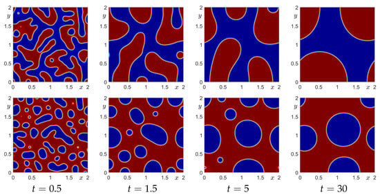
Figure 4. The top and bottom rows display the snapshots of $\varphi$ with respect to $\overline{\varphi }=0$ and $0.3$. The computational moments are illustrated under each figure.

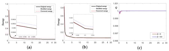
Figure 5. Evolutions of energy curves with respect to $\overline{\varphi }=0$ and $0.3$ are shown in (a,b). Evolutions of $Q^n$ under different average concentrations are plotted in (c).

Next, we investigate the flow-coupled nucleation process. The following initial condition of $\varphi$ is used

$$\begin{array}{ccc}\hfill \varphi (x,y,0)& =& y-1+0.01\mathrm{rand}(x,y).\hfill \end{array}$$

(48)

The initial velocity and pressure are zero. The above initial condition indicates that the magnitude of $\varphi$ takes larger value near the upper and lower boundaries and takes smaller value near the domain center. The parameters are unchanged except $\lambda =0.1$. The snapshots of $\varphi$ and velocity field are shown in the top and bottom rows of Figure 6, respectively. We observe that the phase separation occurs in the nearby region of domain center. With time evolution, the formed droplets gradually disappear because the energy dissipation leads to the shrink of total interfacial length. During this process, the energy curves are non-increasing, the mass is conserved, and $Q^n$ is close to 1. These are reflected in Figure 7a–c.

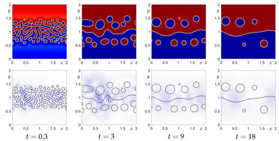
Figure 6. The top and bottom rows display the snapshots of $\varphi$ and velocity field for nucleation process. The computational moments are illustrated under each figure.

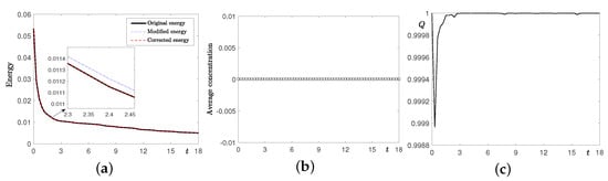
Figure 7. Evolutions of energy curves, average concentration, and $Q^n$ are plotted in (a–c), respectively.

4.4. Droplet Impacting on a Liquid-Liquid Interface

To investigate the capability of our proposed method, we consider a typical two-phase flow problem including the combined effects of surface tension and gravity. For convenience, we assume the density ratio of two fluids is small. The Boussinesq approximation [43] is adopted to recast the momentum equation as

$$\begin{array}{c}\hfill {\rho }_{*}\left(\frac{\partial \mathbf{u}}{\partial t}+\mathbf{u}·\nabla \mathbf{u}\right)=-\nabla p+\frac{1}{Re}\Delta \mathbf{u}-\frac{1}{We}\varphi \nabla \mu +(\rho (\varphi )-{\rho }_{*})\mathbf{g},\end{array}$$

(49)

Here, the background density is ${\rho }^{*}$ and we set ${\rho }^{*}={\rho }_2$. The density functional is $\rho (\varphi )={\rho }_1(1+\varphi )/2+{\rho }_2(1-\varphi )/2$. The gravitational acceleration is $\mathbf{g}=(0,-1)$. Here, we consider ${\rho }_1:{\rho }_2=1.6:1$. The simulation is performed in $\Omega =(0,1)\times (0,4)$. The initial conditions are defined as

$$\begin{array}{ccc}\hfill \varphi (x,y,0)& =& tanh\left(\frac{0.2-\sqrt{{(x-0.5)}^2+{(y-2.4)}^2}}{\sqrt{2}ϵ}\right)+tanh\left(\frac{2-y}{\sqrt{2}ϵ}\right)+1,\hfill \end{array}$$

(50)

$$\begin{array}{ccc}\hfill u(x,y,0)& =& 0,v(x,y,0)=0,p(x,y,0)=0,Q(0)=1.\hfill \end{array}$$

(51)

The parameters are set to be: $\Delta t=0.001$, $h=1/64$, $ϵ=0.015$, $Pe=1/ϵ$, $\lambda =1$, $Re=30$, $We=100$, and $S=2$. The top and middle rows of Figure 8 show the snapshots of $\varphi$ and velocity field at different moments. Here, the red and dark blue regions are occupied by heavier and lighter fluids. Under gravity, the heavier droplet falls. After the impact, the droplet is gradually absorbed into the heavy fluid region. During this process, we find from the bottom row of Figure 8 that $Q^n$ is close to 1.

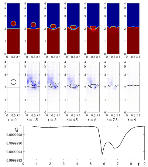
Figure 8. The top and middle rows display the snapshots of $\varphi$ and velocity field. The computational moments are shown under each figure. The bottom row plots the evolution of $Q^n$.

4.5. Dripping Droplet under Gravity

In this subsection, we investigate the dripping droplet under gravity. With the assumption of small density ratio, we still adopt the Boussinesq approximation. The domain is $\Omega =(0,1)\times (0,4)$. The initial conditions are defined to be

$$\begin{array}{ccc}\hfill \varphi (x,y,0)& =& tanh\left(\frac{0.42-\sqrt{{(x-0.5)}^2+{(y-4.2)}^2}}{\sqrt{2}ϵ}\right),\hfill \end{array}$$

(52)

$$\begin{array}{ccc}\hfill u(x,y,0)& =& 0,v(x,y,0)=0,p(x,y,0)=0,Q(0)=1.\hfill \end{array}$$

(53)

The parameters are: $h=1/64$, $\Delta t=0.002$, $ϵ=0.015$, $\lambda =1$, $Pe=1/ϵ$, $Re=30$, $We=1000$, and $S=2$. The density ratio is ${\rho }_1:{\rho }_2=1.6:1$. Under gravity, we can observe the formation of elongated liquid filament. Finally, the pinch-off appears. The snapshots of $\varphi$ are shown in the top row of Figure 9. The middle row displays the velocity field at different moments. The circulation evolves according to the dripping process. From the bottom row, the result indicates that $Q^n$ is close to 1.

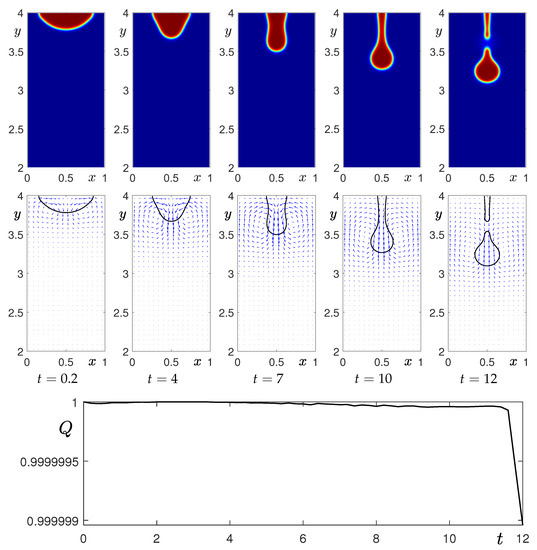
Figure 9. The top and middle rows display the snapshots of $\varphi$ and velocity field for dripping droplet. The computational moments are shown under each figure. The bottom row plots the evolution of $Q^n$.

5. Conclusions

Based on an efficient auxiliary variable approach and a simple energy correction technique, we herein developed a linearly decoupled, second-order time-accurate, and energy-stable scheme for the incompressible CHNS model. Because all variables are decoupled in time, the numerical implementation can be performed in a step-by-step manner. The unique solvability and energy stability in each time step were analytically proved. The fully discrete scheme based on FDM was described in detail. The numerical simulations indicated that the proposed scheme achieved desired second-order accuracy in time. The energy correction technique was essential to enhance the stability and consistency. Furthermore, some typical two-phase flow problems, such as flow-coupled phase separation, falling droplet, and dripping droplet, were well simulated. In the upcoming works, the proposed scheme will be extended for N-phase ($N\ge 3$) fluid systems [44,45,46].

References

- Masiri, S.M.; Bayareh, M.; Nadooshan, A.A. Pairwise interaction of drops in shear-thinning inelastic fluids. Korea-Aust. Rheol. J. 2019, 31, 25–34. [Google Scholar] [CrossRef]
- Goodarzi, Z.; Nadooshan, A.A.; Bayareh, M. Numerical investigation of off-center binary collision of droplets in a horizontal channel. J. Braz. Soc. Mech. Sci. Eng. 2018, 40, 156. [Google Scholar] [CrossRef]
- Lee, C.; Jeong, D.; Yang, J.; Kim, J. Nonlinear multigrid implementation for the two-dimensional Cahn–Hilliard equation. Mathematics 2020, 8, 97. [Google Scholar] [CrossRef]
- Cahn, J.W.; Hilliard, J.E. Free energy of a non-uniform system I: Interfacial free energy. J. Chem. Phys. 1958, 28, 258–267. [Google Scholar] [CrossRef]
- Budiana, E.P. Meshless numerical model based on radial basis function (RBF) method to simulate the Rayleigh–Taylor instability (RTI). Comput. Fluids 2020, 201, 104472. [Google Scholar] [CrossRef]
- Hu, Y.; He, Q.; Li, D.; Li, Y.; Niu, X. On the total mass conservation and the volume presenvation in the diffuse interface method. Comput. Fluids 2019, 193, 104291. [Google Scholar] [CrossRef]
- Liang, H.; Xia, Z.; Huang, H. Late-time description of immiscible Rayleigh–Taylor instability: A lattice Boltzmann study. Phys. Fluids 2021, 33, 082103. [Google Scholar] [CrossRef]
- Chen, J.; Gao, P.; Xia, Y.T.; Li, E.; Liu, H.; Ding, H. Early stage of delayed coalescence of soluble paired droplets: A numerical study. Phys. Fluids 2021, 33, 092005. [Google Scholar] [CrossRef]
- Nishida, H.; Kohashi, S.; Tanaka, M. Construction of seamless immersed boundary phase-field method. Comput. Fluids 2018, 164, 41–49. [Google Scholar] [CrossRef]
- Yang, J.; Li, Y.; Kim, J. A correct benchmark problem of a two-dimensional droplet deformation in simple shear flow. Mathematics 2022, 10, 4092. [Google Scholar] [CrossRef]
- Yang, W.; Huang, Z.; Zhu, W. Image segmentation using the Cahn–Hilliard equation. J. Sci. Comput. 2019, 79, 1057–1077. [Google Scholar] [CrossRef]
- Bartels, A.; Kurzeja, P.; Mosler, J. Cahn–Hilliard phase field theory coupled to mechanics: Fundamentals, numerical implementation and application to topology optimization. Comput. Methods Appl. Mech. Eng. 2021, 383, 113918. [Google Scholar] [CrossRef]
- Khain, E.; Sander, L.M. Generalized Cahn–Hilliard equation for biological applications. Phys. Rev. E 2008, 77, 051129. [Google Scholar] [CrossRef] [PubMed]
- Jeong, D.; Kim, J. A phase-field model and its hybrid numerical scheme for the tissue growth. Appl. Numer. Math. 2017, 117, 22–35. [Google Scholar] [CrossRef]
- Guo, J.; Wang, C.; Wise, S.; Yue, X. An H2 convergence of a second-order convex-splitting, finite difference scheme for the three-dimensional Cahn–Hilliard equation. Commun. Math. Sci. 2016, 14, 489–515. [Google Scholar] [CrossRef]
- Chen, W.; Liu, Y.; Wang, C.; Wise, S. Convergence analysis of a fully discrete finite difference scheme for Cahn–Hilliard–Hele–Shaw equation. Math. Comput. 2016, 85, 2231–2257. [Google Scholar] [CrossRef]
- Diegel, A.; Wang, C.; Wise, S. Stability and convergence of a second order mixed finite element method for the Cahn–Hilliard equation. IMA J. Numer. Anal. 2016, 36, 1867–1897. [Google Scholar] [CrossRef]
- Lee, S.; Shin, J. Energy stable compact scheme for Cahn–Hilliard equation with periodic boundary condition. Comput. Math. Appl. 2019, 77, 189–198. [Google Scholar] [CrossRef]
- Shen, J.; Xu, J.; Yang, J. The scalar auxiliary variable (SAV) approach for gradient flows. J. Comput. Phys. 2018, 353, 407–416. [Google Scholar] [CrossRef]
- Zhang, C.; Ouyang, J.; Wang, C.; Wise, S.M. Numerical comparison of modified-energy stable SAV-type schemes and classical BDF methods on benchmark problems for the functionalized Cahn–Hilliard equation. J. Comput. Phys. 2020, 423, 109772. [Google Scholar] [CrossRef]
- Mu, K.; Si, T.; Li, E.; Xu, R.; Hang, D. Numerical study on droplet generation in axisymmetric flow focusing upon actuation. Phys. Fluids 2018, 30, 012111. [Google Scholar] [CrossRef]
- Huang, B.; Liang, H.; Xu, J. Lattice Boltzmann simulation of binary three-dimensional droplet coalescence in a confined shear flow. Phys. Fluids 2022, 34, 032101. [Google Scholar] [CrossRef]
- Korkmaz, F.C. Damping of sloshing impact on bottom-layer fluid by adding a viscous top-layer fluid. Ocean Eng. 2022, 254, 111357. [Google Scholar] [CrossRef]
- Lee, H.G.; Kim, J. Numerical simulation of the three-dimensional Rayleigh–Taylor instabilty. Comput. Math. Appl. 2013, 66, 1466–1474. [Google Scholar] [CrossRef]
- Li, X.; Shen, J. On fully decoupled MSAV schemes for the Cahn–Hilliard–Navier–Stokes model of two-phase fncompressible flows. Math. Model Meth. Appl. Sci. 2022, 32, 457–495. [Google Scholar] [CrossRef]
- Ye, Q.; Ouyang, Z.; Chen, C.; Yang, X. Efficient decoupled second-order numerical scheme for the flow-coupled Cahn–Hilliard phase-field model of two-phase flows. J. Comput. Appl. Math. 2022, 405, 113875. [Google Scholar] [CrossRef]
- Li, M.; Xu, C. New efficient time-stepping schemes for the Navier–Stokes–Cahn–Hilliard equations. Comput. Fluids 2021, 231, 105174. [Google Scholar] [CrossRef]
- Liu, Z.; Li, X. A highly efficient and accurate exponential semi-implicit scalar auxiliary variable (ESI-SAV) approach for dissipative system. J. Comput. Phys. 2021, 447, 110703. [Google Scholar] [CrossRef]
- Zheng, N.; Li, X. New efficient and unconditionally energy stable schemes for the Cahn–Hilliard–Brinkman system. Appl. Math. Lett. 2022, 128, 107918. [Google Scholar] [CrossRef]
- Yang, J.; Kim, J. Numerical study of the ternary Cahn–Hilliard fluids by using an efficient modified scalar auxiliary variable approach. Commun. Nonlinear Sci. Numer. Simulat. 2021, 102, 105923. [Google Scholar] [CrossRef]
- Jiang, M.; Zhang, Z.; Zhao, J. Improving the accuracy and consistency of the scalar auxiliary variable (SAV) method with relaxation. J. Comput. Phys. 2022, 456, 110954. [Google Scholar] [CrossRef]
- Zhang, Y.; Shen, J. A generalized SAV approach with relaxation for dissipative systems. J. Comput. Phys. 2022, 464, 111311. [Google Scholar] [CrossRef]
- Kim, J. Phase-field models for multi-component fluid flows. Commun. Comput. Phys. 2012, 12, 613–661. [Google Scholar] [CrossRef]
- Zhu, G.; Chen, H.; Yao, J.; Sun, S. Efficiet energy-stable schemes for the hydrodynamics coupled phase-field model. Appl. Math. Model 2019, 70, 82–108. [Google Scholar] [CrossRef]
- Yang, J.; Kim, J. An efficient stabilized multiple auxiliary variables method for the Cahn–Hilliard–Darcy two-phase flow system. Comput. Fluids 2021, 223, 104948. [Google Scholar] [CrossRef]
- Harlow, F.H.; Welch, J.E. Numerical calculation of time-dependent viscous incompressible flow of fluid with free surface. Phys. Fluids 1965, 8, 2182–2189. [Google Scholar] [CrossRef]
- Jeong, D.; Kim, J. Conservative Allen–Cahn–Navier–Stokes system for incompressible two-phase fluid flows. Comput. Fluids 2017, 156, 239–246. [Google Scholar] [CrossRef]
- Zhu, G.; Chen, H.; Li, A.; Sun, S.; Yao, J. Fully discrete energy stable scheme for a phase-field moving contact line model with variable densities and viscosities. Appl. Math. Model 2020, 83, 614–639. [Google Scholar] [CrossRef]
- Pan, X.; Kim, K.H.; Choi, J.I. Monolithic projection-based method with staggered time discretization for solving non-Oberbck–Boussinesq natural convection flows. J. Comput. Phys. 2022, 463, 111238. [Google Scholar] [CrossRef]
- Kim, J. An augmented projection method for the incompressible Navier–Stokes equations in arbitrary domains. Int. J. Comput. Method 2005, 2, 1–12. [Google Scholar] [CrossRef]
- Lee, C.; Jeong, D.; Shin, J.; Li, Y.; Kim, J. A fourth-order spatial accurate and practically stable compact scheme for the Cahn–Hilliard equation. Physica A 2014, 409, 17–28. [Google Scholar] [CrossRef]
- Choi, J.W.; Lee, H.G.; Jeong, D.; Kim, J. An unconditionally gradient stable numerical method for solving the Allen–Cahn equation. Physica A 2009, 388, 1791–1803. [Google Scholar] [CrossRef]
- Lee, H.G.; Kim, J. A comparison stusy of the Boussinesq and the full variable density models on buoyancy-driven flows. J. Eng. Math. 2012, 75, 15–27. [Google Scholar] [CrossRef]
- Aihara, S.; Takaki, T.; Takada, N. Multi-phase-field modeling using a conservative Allen–Cahn equation for multiphase flow. Comput. Fluids 2019, 178, 141–151. [Google Scholar] [CrossRef]
- Yang, J.; Lee, C.; Kim, J. Reduction in vacuum phenomenon for the triple junction in the ternary Cahn–Hilliard model. Acta Mech. 2021, 232, 4485–4495. [Google Scholar] [CrossRef]
- Haghani-Hassan-Abadi, R.; Rahimian, M.H. Axisymmetric lattice Boltzmann model for simulation of ternary fluid flows. Acta Mech. 2020, 231, 2323–2334. [Google Scholar] [CrossRef]
Publisher’s Note: MDPI stays neutral with regard to jurisdictional claims in published maps and institutional affiliations. |
© 2022 by the authors. Licensee MDPI, Basel, Switzerland. This article is an open access article distributed under the terms and conditions of the Creative Commons Attribution (CC BY) license (https://creativecommons.org/licenses/by/4.0/).