Article

A Method of Optimizing Cell Voltage Based on STA-LSSVM Model

1
School of Automation, Guangdong Polytechnic Normal University, Guangzhou 510665, China
2
Guangzhou Intelligent Building Equipment Information Integration and Control Key Laboratory, Guangzhou 510665, China
*
Author to whom correspondence should be addressed.
Mathematics 2022, 10(24), 4710; https://doi.org/10.3390/math10244710
Submission received: 19 October 2022 / Revised: 3 December 2022 / Accepted: 8 December 2022 / Published: 12 December 2022
(This article belongs to the Special Issue Advanced Control Theory with Applications)

Abstract

:
It is challenging to control and optimize the aluminum electrolysis process due to its non-linearity and high energy consumption. Reducing the cell voltage is crucial for energy consumption reduction. This paper presents an intelligent method of predicting and optimizing cell voltage based on the evaluation of modeling the comprehensive cell state. Firstly, the Savitzky–Golay filtering algorithm(SGFA) is adopted to denoise the sample data to improve the accuracy of the experimental model. Due to the influencing factors of the cell state, a comprehensive evaluation model of the cell state is established. Secondly, the model of the least squares supports vector machine (LSSVM) is proposed to predict the cell voltage. In order to improve the accuracy of the model, the state transition algorithm (STA) is employed to optimize the structure parameters of the model. Thirdly, the optimization and control model of the cell voltage is developed by an analysis of the technical conditions. Then, the STA is used to realize the optimization of the front model. Finally, the actual data were applied to the experiments of the above method, and the proposed STA was compared with other methods. The results of experiments show that this method is efficient and satisfactory. The optimization value of average cell voltage based on the STA-LSSVM is 3.8165v, and it can be used to guide process operation. The DC power consumption is 11,971 KW·h per tonne of aluminum, with a reduction in power consumption of 373 KW·h. This result guarantees the reduction of aluminum electrolysis energy consumption.

1. Introduction

The aluminum electrolysis industry uses an enormous amount of electricity, with electricity costs accounting for 30–40% of the total production costs. Aluminum electrolysis production becomes more expensive as the cost of electricity rises. As a result, one of the primary goals of aluminum factories is to achieve energy-efficient production in aluminum electrolysis [1,2]. The primary approach to energy reduction is to reduce the DC power in the aluminum electrolysis process. Academic and industry researchers have conducted various studies. Lan et al. [3] analyzed the effects of aluminum level, alumina concentration, cell temperature, mole ratio, and noise value on current efficiency and proposed a theoretical method to improve current efficiency by optimizing the relevant technical conditions. Li et al. [4] proposed a modal analysis method to clarify how the anode-cathode distance (ACD) and length–width ratio of cells affected interfacial stability; the results indicate that the stability is enhanced as the increase of ACD for a 500-KA electrolysis cell and the critical ACD is derived as 0.041 m, which is preferable for stabilizing the cell and reducing energy consumption. Tu et al. [5] proposed a monitoring method of equivalent series resistance (ESR) and capacitance to stabilize aluminum electrolytic production by timely detection of problematic aluminum electrolytic capacitors and indirectly improve the current efficiency. The theoretical methods to reduce the DC power consumption of aluminum electrolysis are proposed in the above literature. However, with the development of modern process digitization, the above-mentioned methods have become difficult to apply to modern aluminum electrolysis processes.
Aluminum electrolysis production is a high-energy, non-linear process with many parameters that affect the cell state during operation. These parameters are an important basis for determining the current state of the aluminum electrolytic cell. When the cell state is good, the production is stable, the current efficiency is high, and the probability of failure is low. Therefore, determining the aluminum electrolytic cell state is necessary. To address the challenge of classifying cell state, Zhang et al. [6] used current efficiency as a basis for evaluating cell state. Cui et al. [7] simply divide the aluminum electrolytic cell state into a cold stroke, normal, and hot stroke according to the temperature range of different cells. Lin et al. [8] extracted the features of the cell state from the cell voltage transient curve and used an artificial neural network for cell state diagnosis. Most of the current methods of classifying cell states are based on single indicators, such as current efficiency, electrolyte temperature, and instantaneous voltage, without judging it from a global perspective.
With the development of modern industrial digitization, data mining is widely used for complex industrial control. Fan et al. [9] proposed an NSGA-II algorithm based on a function-based evolutionary operator and obtained the optimal set of Pareto solutions with uniform distribution to achieve the purpose of efficiency and consumption reduction. Li et al. [10] proposed a multi-objective optimal control strategy based on quantum optimization to optimize the current efficiency and DC power consumption of the aluminum electrolysis process. Xu et al. [11] established a genetic algorithm-multiple extreme learning machine (ELM) based model for optimizing the cell voltage in the electrolytic aluminum production process to reduce power consumption. Yi et al. [12] built a deep learning-based anode effect prediction model to optimize aluminum electrolysis production. These research methods have poor practicality and do not better reduce energy consumption.
During actual production, when the cell state is poor, the operator can change the electrolytic cell from poor to excellent by adjusting the process parameters, and when the cell is in a good state, energy consumption can be further reduced by reducing the cell voltage. The relationship between the cell voltage and the relevant technical conditions cannot simply be modeled by mathematical expressions [13]. LSSVM [14], an extension of support vector machine (SVM) [15], exhibits good generalization performance, low computational complexity, and high prediction accuracy, which is suitable for non-linear, high-dimensional, and small sample application scenarios. The cell voltage prediction model using this algorithm can well describe the relationship between cell voltage and technical conditions. Currently, researchers usually optimize the LSSVM parameters [16,17,18,19] or construct suitable kernel functions [20,21,22] to improve the performance of LSSVM algorithms. STR is a new intelligent optimization algorithm proposed by Dr. Zhou in 2012 [23,24]. This algorithm is a new intelligent randomness global optimization algorithm, compared with some algorithms that are easy to fall into local optimality and have a general search range. The algorithm aims to solve optimization problems and find the optimal global solution or the approximate optimal solution [25,26]. However, these methods only provide the analysis of cell state and produce good results in dealing with the problem of a single objective optimization. This makes it difficult to obtain satisfactory optimization.
In the aluminum electrolysis process, simply reducing cell voltage without considering other parameters can affect the current efficiency and stability of the electrolytic cell. This will result in decreasing the amount of product in the electrolysis process. So, this paper explains a comprehensive model of evaluating the cell state and presents a method of optimizing the cell voltage from a global perspective. First, applying the data of actual aluminum production, in this paper, the cell state was divided into excellent, good, and poor cell states based on K-means++. In order to improve the accuracy of the cell state evaluation model, SGFA was used to remove noise from the original data. The experimental results show that the evaluation model has high accuracy. In the case of a good cell state, the cell voltage is modeled by the LSSVM, and the model parameters are optimized by STA. To verify the effectiveness of the model, we compared the optimized LSSVM with the traditional LSSVM, backpropagation (BP) neural network, and extreme learning machines (ELM). After achieving the cell voltage estimation model, a cell voltage optimization model was constructed, then the STA was applied to optimize cell voltage and search for a set of optimized operation parameters, which can make the cell state turn to the optimal state. The optimal cell voltage can reach 3.8165 v, and the direct consumption per ton of aluminum production can be reduced by 373 KW·h in theory. These results demonstrate the validity of the method.

2. Data Processing Based on DBSCAN Algorithm

2.1. The Processing of Aluminum Electrolysis

Charles Martin Hall and Paul Heroult invented a method for the electrolysis of primary aluminum, which is the only method of producing metallic aluminum in the contemporary industry [27]. An electrolytic cell is an aluminum electrolysis reaction device, mainly divided into electrical insulation, cathode structure, superstructure, and busbar structure; the schematic diagram of an electrolytic cell is depicted in Figure 1. With carbon material as two poles and alumina-cryolite melting as an electrolyte, the electrochemical reaction is carried out on the two poles in the electrolytic cell after a strong direct current is applied. Aluminum ions are released after the addition of alumina dissolution, while an electrochemical reaction occurs near the anode to generate intermediate products, which react with the carbon anode as shown in Equation (1). Under the electrolyte layer, there is a layer of liquid aluminum, which is set in a performed carbon liner. At this time, the number of aluminum cations at the metal/electrolyte interface gradually decreases, and a reduction reaction takes place. The reaction is shown in Equation (2). Equation (3) presents the total reaction. The electrochemical reaction between molten alumina and carbon during electrolysis produces liquid aluminum and gaseous carbon dioxide, the exhaust gas is purified and vented, and the recovered fluoride is returned to the electrolytic cell [28].
On the anode:
3 O 2 + 1 . 5 C - 6 e = 1 . 5 CO 2
On the cathode:
2 Al 3 + + 6 e = 2 Al
The total reaction:
AL 2 O 3 + 1.5 C = 2 Al + 1.5 CO 2
The work conducted by the current is the product of current, voltage, and time. Under the premise of a certain current, the DC power consumption = 2980 * (average cell voltage)/(current efficiency). The energy consumption of aluminum electrolysis is closely related to cell voltage; the lower the voltage, the lower the power consumption. So it is crucial to control the cell voltage in production. The reduction of energy consumption is achieved by controlling the production of aluminum electrolysis at low voltage under good cell conditions in this paper and a certain current.

2.2. Experimental Data Preprocessing

Due to the inherent defects of the electrolysis cell acquisition equipment and the changes in the production environment of the cell, the collected data signal is always inevitably contaminated by noise. The accuracy cannot be satisfying if the signal is fed to the model without denoising. In this subsection, the SGFA is used to denoise the aluminum electrolysis data. The SGFA is improved from the moving smoothing algorithm proposed by Savitzky and Golay [29] and is also called local least squares polynomial-based smoothing [30]. It has been widely used in various fields of data smoothing and denoising since its publication [31,32,33]. This algorithm can remove noise while preserving the information of the original data signal and the shape of the curve. The expression of SGFA, which is essentially window sliding convolution, is as follows.
y ^ i = j = n n ω j y i + j
where y ^ i ( i = 1 , , N ) is the result of SGFA, ω j ( j = n , , n ) is the SGFA weight, y i + j is the corresponding original time signal value, n is the half window size of SGFA, ω j is calculated using a local least squares fit of a polynomial function over the window.
f ( t ) = c 1 φ 1 ( t ) + c 2 φ 2 ( t ) + + c M φ M ( t )
where φ 1 ( t ) , φ 2 ( t ) , , φ M ( t ) is the fitted basis function, and the coefficients c 1 , c 2 , , c M can be obtained by (6).
c = ( A T A ) 1 A T b
Considering the size of the computation and the goodness of the fit, Formula (7) is applied to the sliding window to do the fitting operation on the data points in it.
f ( t ) = c 1 + c 2 t + c 3 t 2
where φ 1 ( t ) = 1, φ 2 ( t ) = t, φ 1 ( t ) = t 2 . When the window width is 2 n + 1 , then the matrix A is:
A = [ ω 1 ω 1 t 1 ω 1 t 1 2 ω 2 ω 2 t 2 ω 2 t 2 2 ω 2 n + 1 ω 2 n + 1 t 2 n + 1 ω 2 n + 1 t 2 n + 1 2 ]
According to Formulas (5) and (7)~(9), the SGFA weights in the following equation can be obtained.
w = B ( A T A ) 1 A T d i a g ( ω ) y
where B = [ 1   t i   t i 2 ] is a set of row vectors composed of the corresponding timing points of the SGFA result y i ^ , d i a g ( ω ) is a diagonal matrix composed of ω i weights, y is a vector of 2 n + 1 values among the corresponding sliding window.
Data normalization [34] can improve the efficiency of the algorithm and can reduce the proportion of the distance accounted for by different attributes of overly large values and relatively small initial values in the data domain, so the data were scaled between 0 and 1 to facilitate a comprehensive comparative evaluation of each indicator of the aluminum electrolysis data and to visualize the aluminum electrolysis production. In this paper, the data are de-scaled using Equation (10).
x i * = x i x min x max x min
where x min and x max denote the minimum and maximum values of the parameter variables, x i and x i * denote the data before and after the normalization of the variable, respectively.

3. Cell State Evaluation Analysis Model

3.1. Comprehensive Evaluation Index of Cell State

The aluminum electrolytic cell states show the good or bad production condition of the electrolysis cell, a better cell state indicates higher current aluminum production efficiency, and the aluminum yield and quality can be improved. However, in the process of electrolysis, maintaining the heat balance and material balance of the electrolysis cell are two key factors for the production of aluminum. If the balance is disrupted, the state of the electrolysis cell will develop in the direction of a sick cell, with failures such as hot or cold cell, anode effect, and even accidents, resulting in casualties. Therefore, in order to correctly evaluate the current state of the electrolysis cell and to issue specific instructions for different cell states, a cell state evaluation model based on the K-means++ algorithm is proposed in this paper.
In order to more conveniently and qualitatively determine the cell state, a comprehensive evaluation index d of the cell state, which consists of DC power consumption W and current efficiency η , is defined. The closer the current efficiency is to 100%, the more efficient the electrolysis cell production. The definition of the cell state space is shown in Equation (11).
( u , v ) = ( W W opt W opt , 1 η )
where W opt is the optimized DC power consumption of 12,200 kW per ton of aluminum [35], ( u , v ) is the distance W and η from the ideal state, the distance reflects the level of the cell state, i.e., the closer, the better. The comprehensive evaluation index of the cell state is defined in (12).
d = u 2 + v 2
where the size of d measures the good or bad state of the cell; the closer d is to 0, the better the cell state; the larger d is, the worse the cell state.

3.2. Evaluation Model of Cell State Based on K-Means++ Algorithm

The change of cell voltage in the actual production of electrolysis cell affects the DC power consumption and current efficiency, so it is necessary to control the cell voltage in a reasonable range in order to ensure aluminum production. Noise caused by the anode effect disrupts the balance in the cell. The material balance is the balance between the aluminum fluoride feeding amount and aluminum discharge amount, and the aluminum discharge amount is directly related to the current efficiency calculation formula. If the electrolysis temperature is too high, the current efficiency reduces, and the power consumption increases. It is important to maintain a reasonable level of electrolyte and aluminum because they affect the balance of the thermal field and magnetic field in the cell, which is crucial to the smooth and effective operation of the cell and, eventually, the quantity and quality of aluminum.
To sum up the mechanism analysis, the important process parameters affecting DC power consumption and current efficiency include cell voltage, noise, aluminum fluoride feeding amount, electrolyte temperature, electrolyte level, aluminum level, and aluminum output. In this paper, these parameters are used as the relevant parameters for the cluster evaluation of cell states.
K-means++ algorithm [36], an improved version of the K-means algorithm, follows the principle of “the farther the cluster centers are, the better”. It aggregates data with the same characteristics into clusters and determines the number of clusters efficiently.
(1) Determine the number of clusters. The Elbow method and silhouette coefficient method are both methods to evaluate the clustering effect of the current clustering number K. The value of the current clustering number K can be weighed by the two methods.
The elbow method [37] is also called the error square sum method. Its core idea is that the increase of the clustering classification number K makes the degree of similarity within each class higher and the degree of similarity between classes smaller. When the value of K increases to a certain point, the value of the error square sum drops sharply. When the shape of the inflection point on the SSE and K relationship graph is similar to the elbow, and the curve slope reaches the maximum, the current K value can be preliminarily determined as the best. The calculation formula of the square sum of the elbow method error is shown in Equation (13).
S S E = i = 1 K p C i | p m i | 2
where p is the samples in category i , m i is the mean value of the samples in cluster i .
The silhouette coefficient method is another important method to evaluate the cluster value. The calculation formula is shown in (14). The higher the S ( i ) value, the lower the similarity between clusters, the higher the similarity within clusters, and the better the clustering effect. The highest number of clusters in S ( i ) indicates that the current K value of the cluster is the best choice.
S ( i ) = b ( i ) a ( i ) max { a ( i ) , b ( i ) }
where a ( i ) is the intra-cluster dissimilarity, which refers to the average of the dissimilarity between vector i and each sample point within the cluster, b ( i ) is the inter-cluster dissimilarity, which refers to the minimum of the average dissimilarity of vector i and other clusters, reflecting the degree of separation, and S ( i ) is the silhouette coefficient value.
(2) Select the initial cluster center. This part is the main difference between K-means++ and K-means algorithm. K-means++ algorithm can obtain more satisfying clustering results by setting different locations as aggregation centers with higher probability distance. Assume that the eigenvector samples of n aluminum electrolytic cell state data are U = { u 1 , u 2 , u n } . Each sample is composed of cell state-associated parameter characteristics: u i = [ v i 1 , v i 2 , v i 3 , v i 4 , v i 5 , v i 6 , v i 7 ] , the data samples are divided into K categories, the cluster center of each category is C = { c 1 , c 2 , , c K } , and the composition of each cluster center is c i = [ p i 1 , p i 2 , p i 3 , p i 4 , p i 5 , p i 6 , p i 7 ] .
The realization steps of K-means++ algorithm is described as follows:
Step 1: Randomly select a sample point in the sample group as the initial cluster center z 1 .
Step 2: Calculate the distance D between each sample point u i and the nearest cluster center c k . The calculation Formula (15) is as follows:
D ( u i , c k ) = j = 1 7 ( v i j p k j ) 2
Step 3: Calculate the probability of each sample point being selected as a new cluster center. The calculation formula of probability P is shown in Formula (16), and then select the next cluster center according to the roulette method.
P = D ( u ) 2 u U D ( u ) 2
Step 4: Repeat Step 2 and Step 3 until K initial cluster centers are selected.
(3) Judge the attribution of feature vector samples and update the cluster center. After selecting the initial clustering center C 0 = { c 1 0 , c 2 0 , , c k 0 } , the standard K-means algorithm is used to calculate the Euclidean distance from each feature vector to the aggregation center:
D ( u i , c k 0 ) = j = 1 7 ( v i j p k j ) 2
After calculating the Euclidean distance, each feature vector is assigned to the nearest cluster. After calculating the attribution of each feature sample, the average value of each feature is calculated according to the sample vector in each cluster, and the cluster center C is updated. Repeat the above steps until the change of the cluster center is less than the set threshold, then the clustering ends.
(4) Calculate the value range of d of all cell states according to the clustering results.

4. Optimization of Cell Voltage

4.1. Soft Sensing Modeling of Cell Voltage Based on STA-LSSVM

When the evaluation results of the cell state are excellent and good, energy consumption can be reduced by lowering the cell voltage. In the current electrolytic cell industry, lowering the cell voltage means reducing the pole distance. However, simply reducing the pole distance will definitely affect the current efficiency and stability of the aluminum electrolytic cell and ultimately reduce aluminum production. Therefore, in order to reduce the cell voltage without decreasing the current efficiency, the parameters that affect the cell voltage can only be adjusted within a reasonable range.
There are many cell voltage parameters that affect the change of aluminum electrolysis. Cell resistance and current intensity directly reflect the change in cell voltage. Alumina concentration, electrolyte temperature, and molecular ratio have significant effects on the change of electrolyte conductivity, thus affecting the stability of cell voltage. Moreover, an important reason for the anode effect is that the cell voltage rises rapidly when the alumina concentration is low, which destroys the balance state of the electrolytic cell; The electrode distance is the distance from the anode bottom to the cathode aluminum liquid mirror. It has a direct impact on cell resistance, resulting in cell voltage change. The temperature of the electrolyte is affected by the height of the aluminum liquid. The height of aluminum liquid changes the thermal balance of the electrolytic cell and then changes the voltage stability of the cell; less anode wetted area causes the anode effect, so the electrolyte level needs to be maintained in a reasonable range to prevent the anode effect from affecting the voltage. When the aluminum level is too high, the heat dissipation in the cell increases, causing the cell bottom to become cold, affecting the thermal balance of the cell and thus affecting the cell voltage stability. Based on the above analysis, the parameters that affect the cell voltage ( y ) are the pole distance ( x 1 ), electrolyte level ( x 2 ), cell resistance ( x 3 ), alumina concentration ( x 4 ), aluminum level ( x 5 ), current intensity ( x 6 ), and molecular ratio ( x 7 ).
In this paper, we use the least squares support vector machine to build a cell voltage prediction model. The LSSVM algorithm has a strong classification capability and requires less training time to train non-linear data with a large time delay and strong coupling. Based on the previous research, we found that the STA is better and more effective in reducing energy consumption by comparing the average value of the cell voltage optimized by ALO and STA [38], so we decided to optimize the LSSVM prediction model by STA. The specific aluminum electrolyzer voltage prediction schematic is shown in Figure 2.
STA treats a solution to the optimization problem as a state and finds the optimal solution by iterating and updating the state, which is regarded as a state transition process. The STA framework is shown as follows:
{ x k + 1 = A k x k + B k u k y k + 1 = f ( x k + 1 )
where x k = [ x 1 , x 2 , , x n ] T is a current state, it represents a candidate solution of the current optimization scheme, A k or B k is a state transition matrix with randomness and an operator of the basic state transition algorithm, u k is a function of x k containing historical state; f ( ) is the objective function or evaluation function; y k is the fitness function value at point x k .
The state transfer-based optimization-seeking algorithm uses four state transformation operators [39], including rotation transformation, translation transformation, expansion transformation, and axial transformation, to solve a continuous optimization problem through evolution.
(1)
(rotation transformation, RT):
x k + 1 = x k + α 1 n x k 2 R r x k
(2)
(translation transformation, TT):
x k + 1 = x k + β R t x k x k 1 x k x k 1 2
(3)
(expansion transformation, ET):
x k + 1 = x k + γ R e x k
(4)
(axesion transformation, AT):
x k + 1 = x k + δ R a x k
where x k R n , α are the rotation factor, β is the translation factor, γ and δ are the stretch factor and coordinate factor, respectively. They are all positive numbers greater than zero. R r R n × n is a random matrix whose elements obey a uniform distribution of [−1,1], x k 2 is a Euclidean or 2-parametric number; R t R is a random variable whose elements obey a uniform distribution between [ 0 , 1 ] . The translation transformation is an algorithm for a line search, mainly along the vector direction from x k 1 to point x k and with x k as the starting point for a line search of maximum length β . R e R n × n is a random diagonal array whose internal elements follow a standard normal distribution. R a R n × n represents a random diagonal sparse matrix with non-zero elements only at one position and the elements absolutely obeying the standard normal distribution. Finally, for the properties of these four operators: the rotation transform is able to control the accuracy of the solution and accomplish the performance of the local search. It guarantees the optimal solution within a hypersphere of maximum radius α . The translation transform not only balances the local search and the global search but also refines the one-dimensional search. The stretching transformation is theoretically able to stretch each element in x k to the range of ( , + ) , allowing a global search to be completed.
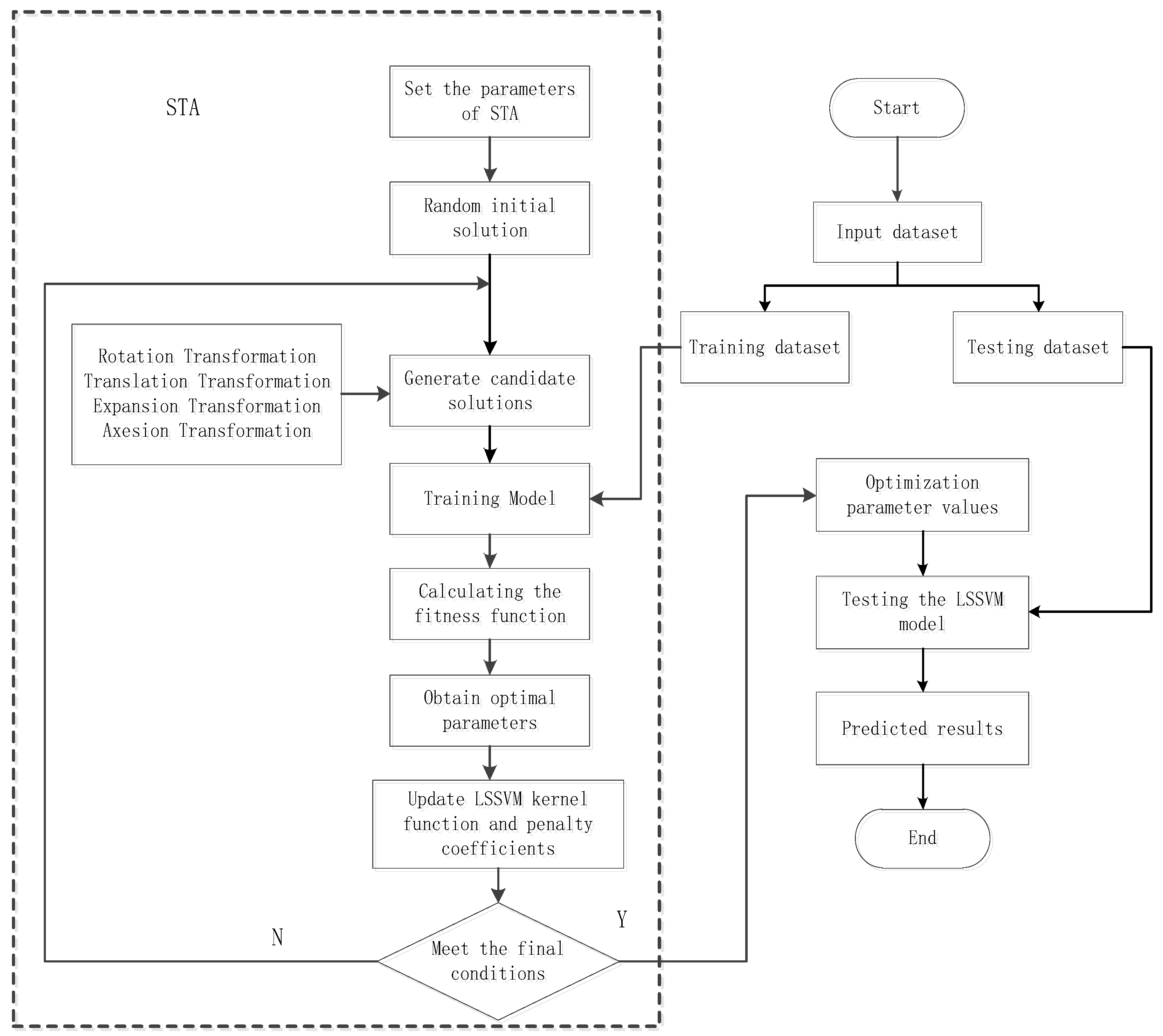
The parameters of LSSVM should be chosen reasonably for the reasons that these parameters uniquely define a specific model and, at the same time, determine the model’s precision that greatly affects the accuracy and effectiveness of cell voltage optimization. In this paper, with RBF is chosen as the kernel function of LSSVM, there are only two parameters that need to be determined, the kernel function’s parameter σ and punishment factor γ . The STA algorithm is used to find the optimal parameters for better learning performance of LSSVM.
The realization steps of the STA-LSSVM algorithm are as follows:
Step 1: The input training set is divided into a training set and a test set.
Step 2: The parameters of the LSSVM model, the parameter σ of the Gaussian radial basis kernel function, and the punishment factor γ , are used as the two merit-seeking parameters to be identified for each set of the state transfer algorithm.
Step 3: Set STA parameters, such as iteration number and search enforcement (SE), Rotation factor α , translation factor β , expansion factor and coordinate factor δ .
Step 4: Generate the initial solution. Each solution of STA represents the combination option of two parameters ( σ , γ ) that determine the LSSVM performance.
Step 5: During each iteration, the STA uses four operational operators in turn to generate candidate solutions, and the solution with a better fitness value for the training set is reserved for the next iteration.
Step 6: If the termination condition is met, the algorithm optimization process stops, and the LSSVM model training is completed. If the termination condition is not met, return to Step 5.
Step 7: In the test dataset, the STA-LSSVM model was used to predict the cell voltage and output the prediction results.
The flow chart of STA-LSSVM to build a cell voltage prediction model implementation is shown in Figure 3.

4.2. Cell Voltage Optimization Model Based on STA

After the LSSVM prediction model is established, to realize the optimal control of the cell voltage and achieve the purpose of consumption reduction, it is necessary to find the optimal cell voltage y and its corresponding optimal technical conditions X under normal operating conditions.
Under normal operating conditions, the adjustment of the pole distance is an important tool for regulating the energy balance of the cell. The variation in the length of the pole distance directly affects the cell voltage. In various types of electrolytic cells, the pole distance is generally kept between 3.6~5 cm; a very important condition for the stable and efficient operation of electrolytic cells in aluminum production is to maintain a reasonable electrolyte level, which is between 14~23 cm. The alumina concentration represents the material balance in the cell and ranges from 1.9%~3.5%; in the production of aluminum electrolysis, the aluminum level can significantly affect the current efficiency. The molecular ratio is used to measure the acidity and alkalinity of the electrolyte and is traditionally characterized by the molecular ratio of NaF to AlF3. The molecular ratio should be maintained in the range of 2.1~2.7 and should not be at a lower level. In summary, the seven variables for the mechanistic analysis are set as pole distance ( x 1 ), electrolyte level ( x 2 ), cell resistance ( x 3 ), alumina concentration ( x 4 ), aluminum level ( x 5 ), current intensity ( x 6 ), molecular ratio ( x 7 ), and the optimal control model for cell voltage is established as shown in Equation (23).
Based on the above analysis, the mathematical description of the optimization model can be stated as follows:
min y = g ( x 1 , x 2 , x 3 , x 4 , x 5 , x 6 , x 7 ) s . t . { 3.9 x 1 5 18 x 2 22 11 x 3 13 0.015 x 4 0.035 20 x 5 28 171 x 6 174 2.1 x 7 2.7
The objective of Formula (15) is to find the lowest value of cell voltage under the seven constraints obtained from process analysis and gray correlation analysis, which can be regarded as a multi-objective optimization problem with multiple constraints. In this paper, STA is used to optimize the cell voltage optimization control model. Its optimization steps are:
Step 1: Random initialisation. Set the basic parameters of the algorithm and randomly generate SE = 50 states within a set range, each state representing a set of 7 × 1 cell voltage parameters.
Step 2: Using the cell state parameters in each initial state as input to the cell voltage prediction model, the fitness function value for each initial state is obtained, and the state with the lowest fitness value is taken as the current optimal set parameter value, with the corresponding fitness value taken as the optimal cell voltage.
Step 3: The iteration starts. The state is transformed according to the four optimization operators of the STA, and the value of the fitness function is calculated for the transformed state. The current state is changed only when the optimal value is obtained, updating the cell voltage value and the optimal setting parameters; otherwise, the optimal state is maintained.
Step 4: Determine if the difference between the adaptation value is less than the set threshold or if the maximum number of iterations is 1000, the algorithm ends if one of these criteria is met and the cell voltage optimization value y * is obtained; otherwise, go to Step 3.
The flowchart of optimization based on STA cell voltage is shown in Figure 4.

5. Analysis of Experimental Results

5.1. Data Clustering Analysis

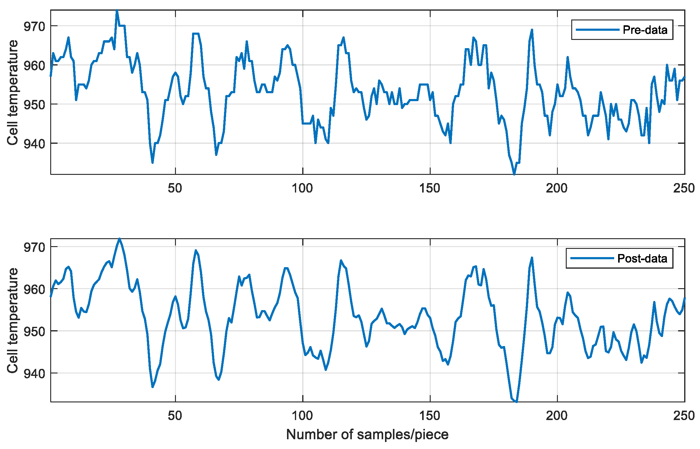
The experiments were carried out on a platform of MATLAB2020a. Moreover, the data used in these experiments were collected from an aluminum factory in China. The accuracy of the experimental model can be improved by using SGFA to denoise the temperature data of the aluminum electrolytic cell.
The time-domain waveform in Figure 5 shows the comparison of results before and after noise removal. There are slight burrs on the curve before data preprocessing. After the SGFA filters the noise, the curve becomes smooth, the random error is reduced, and the side effects of noise on the model convergence speed and accuracy are eliminated.

5.2. Cell State Evaluation

After preprocessing and normalizing the data samples, the cell state is evaluated to obtain a cell state evaluation standard based on comprehensive indicators. After the elbow method and silhouette coefficient method have determined that the optimal cluster number is three categories, the production data is divided into three cell states according to the principle that the cluster centers of the K-means++ algorithm should be as far apart as possible, and the final cluster centers are determined through continuous iteration. The parameter indexes of each cluster center are shown in Table 1.
When the number of clusters is set to three categories, the degree of sample division is high. Among 276 samples, 96 samples are classified as Class 1, at this time, d is the smallest, and they are rated as excellent cells; 102 samples are classified as Class 2, and d value is in the middle, and they are rated as good cell; 78 samples are classified as Class 3, and d is the larger value, which is rated as a poor cell. The comprehensive indicator of cell state is used to evaluate the cell state of each category. Through the indicator, we can classify the cell state data collected in real-time. The specific cell state evaluation results are shown in Table 2.
After the clustering analysis of samples, the coordinate system is established based on three characteristics of normalized electrolyte level, electrolyte temperature, and aluminum output, and the clustering distribution is shown in Figure 6. It can be seen that three colors represent different cell state cluster groups. Samples can be clearly divided into three clusters in high-dimensional space, showing a good clustering effect.
After obtaining the training sample cluster center in Table 1, we verify the cell state evaluation model with 40 additional groups of data and calculate the Euclidean distance between the on-site data samples and the cluster center of the three cell states. The current calculation sample is put to the class whose cluster center is the nearest. Note that the sample classification cell state is the real cell state at this time. The predicted cell state of the sample at this time is evaluated according to the comprehensive evaluation parameter d of the cell state of the sample if the evaluation parameter d of the cell state of the sample is not in the range of cell state evaluation. While the current sample prediction cell state should be categorized into the class using Table 1 by judging which type of d value is the closest to the test sample. The final experimental results are shown in Table 3.
Table 3 shows that in the verification experiment of 40 groups of sample data, the cell state of one Class 1 data was wrongly judged, 39 groups were judged correctly, and the final accuracy rate was 97.5%.

5.3. Prediction of Cell Voltage

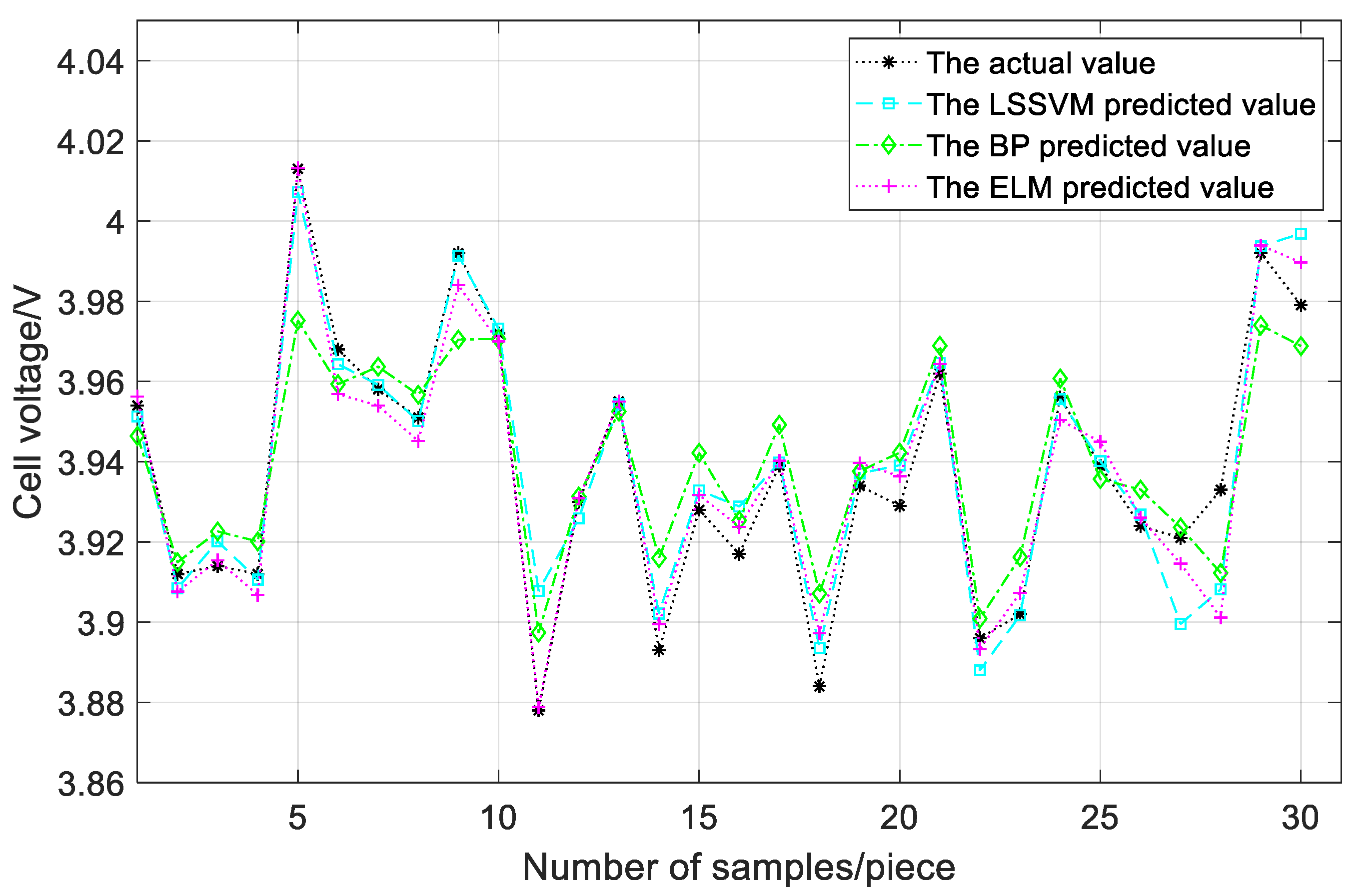
The STA-LSSVM model, LSSVM model, BP model, and ELM model are used to predict the cell voltage respectively and compared with the expected value.
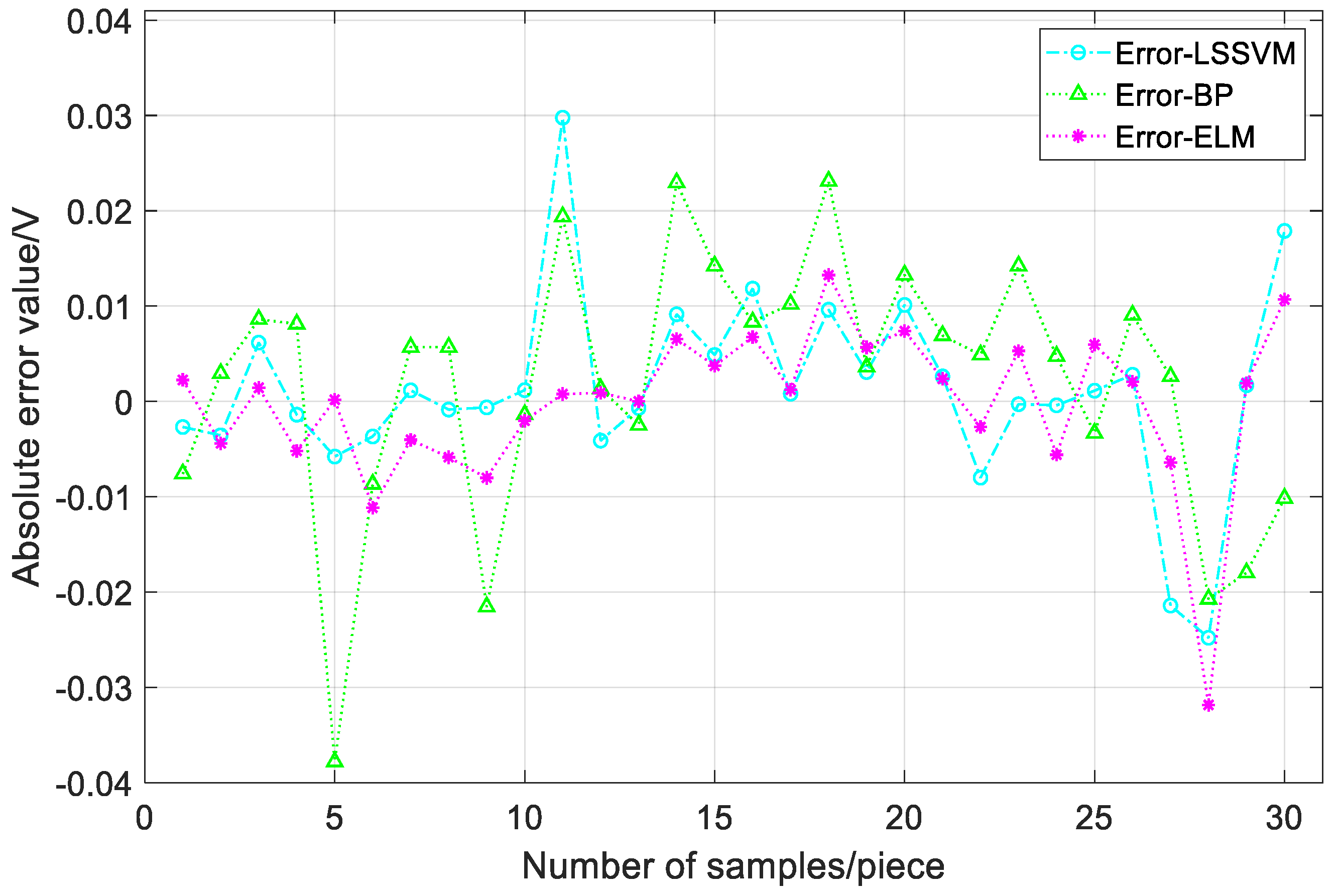
In order to verify the prediction performance of STA-LSSVM, LSSVM before optimization, ELM, and BP neural network, were used to compare with it in this paper. The experimental data were obtained from an aluminum factory in China, and the cell states were all excellent or good. A total of 165 sets of training data and 30 sets of test data were used to train and validate the STA-LSSVM model, respectively. The seven indicators were used as input data and will be used as output data to train the LSSVM model. The parameters of each model are: the empirical method selects the LSSVM kernel function parameter is 20, and the punishment coefficient is 20; the extreme learning machine has 15 hidden layers and the activation function the Sigmoid function; the BP neural network has 5 hidden layers and a learning rate of 0.1 and a training number of 100 rounds with a target threshold of 0.00001. The structure of the LSSVM after STA optimization parameters was ( σ , γ ) = ( 80.6 , 46.8 ) . In order to predict the accuracy of the model prediction, the mean absolute error (MAE) and mean square error (MSE), and the coefficient of determination (R2) was selected as evaluation criteria in this paper to judge the prediction and regression effect comprehensively. The model’s prediction result curve is shown in Figure 7 and Figure 8. The performance evaluation indicators and the prediction result indicators are shown in Table 4.
From Figure 7 and Figure 8, it can be seen that the LSSVM model without STA optimization has a poor prediction effect. For better prediction of cell voltage, this paper optimizes the LSSVM prediction model using the STA algorithm. We compared the results with ALO-LSSVM, BP, ELM, and LSSVM, as shown in Table 4.
As can be seen from the accuracy indicators in Table 4, the STA-LSSVM inherited the learning ability and the robustness of the LSSVM. The method outperforms the other algorithms in terms of MAE, MSE, and R2 evaluation indexes. It has a better fit and can accurately determine the trend of the true value. The results show that the proposed model has good prediction accuracy and can be used for the optimization of aluminum electrolytic voltage.
In summary, the cell voltage soft-measurement model established by STA-LSSVM has better learning ability and generalization ability and has higher precision, which can accurately predict the cell voltage of the aluminum electrolysis process.

5.4. Optimization of Cell Voltage

In the cell voltage prediction experiment, the optimal LSSVM parameters ( σ , γ ) = ( 80.6 , 46.8 ) are obtained after training. In order to further verify the effectiveness and stability of the STA algorithm, the cell voltage was optimized 30 times separately by STA, ALO, SCA, and GWO. Then, the experimental results are compared in Figure 9 and Table 5. V represents the average value of the optimized voltage, S t d represents the standard deviation.
As we can see in Figure 9 and Table 5 hat the cell voltage optimized by ALO, SCA and GWO is not only larger but also has more fluctuation than STA, which indicates that ALO, SCA, and GWO are more likely to obtain the optimal local solution during the process of searching for optimal cell voltage. Therefore, when aiming at the optimization problem of cell voltage, STA has a better searching ability than ALO, SCA, and GWO. After the experiment, the technical conditions of the optimized cell voltage by STA are shown in Table 6. y* is value of optimal cell voltage, and xi* (i = 1,…7) is the corresponding technical condition.
The average current efficiency in the actual production process of the electrolysis cell is about 95%. The DC power consumption = 2980 * (average cell voltage)/(current efficiency), assuming that the actual production maintains the optimal cell voltage value of the experimental results, the DC power consumption value can be calculated using the DC power consumption equation with a current efficiency of 95%. Table 7 shows the DC power consumption before and after optimization.
The cell voltage optimization method proposed in this paper has a DC power consumption of 11,971 KW·h per tonne of aluminum, with a reduction in power consumption of 373 KW·h, while maintaining the same current efficiency for energy saving and consumption reduction. Given the fact that in the aluminum electrolysis process, with the cell life increasing and the electrolysis conditions varying, an aluminum electrolytic cell will change accordingly. These impact the mapping relations between cell voltage and relevant technical conditions. Therefore, in order to maintain self-adaptability, the cell voltage estimation model should be updated and optimized regularly.

6. Discussion

In the era of industrial digitalization, using data mining technology to control cell voltage optimally can significantly improve aluminum electrolysis production efficiency and make the aluminum electrolysis process more intelligent. In this work, we aim to reduce energy consumption by reducing the cell voltage and maintaining a certain DC current while the aluminum electrolytic cell is in good condition. The experimental results show that the energy consumption of aluminum electrolysis production can be significantly reduced through this method.
The DC power consumption of the aluminum electrolysis production process is directly related to the average cell voltage and current efficiency. The energy consumption is reduced by optimizing the relevant technical conditions to improve the current efficiency [3,5,10]. With the development of modern industrial digitalization, by establishing an optimal control model of the cell voltage and optimizing the cell voltage in the electrolytic aluminum production process, production can be optimized [11,12]. Under the condition that the average voltage is as small as possible and the current efficiency is as large as possible, the consumption reduction of aluminum electrolysis can be achieved. At the same time, based on the findings from the literature review and our experiment, we know that the cell voltage can only be reduced to a certain limit. Only when the voltage is reduced and the cell condition is kept in a good state can the stable and reduced consumption production of aluminum electrolysis be achieved.
In real production, aluminum electrolysis data collection can be difficult, which leads to uneven distribution of experimental samples or even unlabeled data. In the follow-up study, we can consider conducting aluminum electrolysis data augmentation experiments to better solve the problems of uneven samples and unlabeled learning. In addition, we should continue the in-depth analysis of cell voltage and look for a better cell voltage design scheme.

7. Conclusions

With the research on saving energy by optimizing the cell voltage as the background, this paper proposes a method to optimize cell voltage based on the cell voltage estimation model. Because it is difficult to select parameters for LSSVM, the STA is adopted to optimize the parameters of LSSVM by establishing the cell voltage estimation model. In addition to improving the accuracy of the cell voltage estimate model, our method thoroughly synthesizes the learning and generalization capabilities of LSSVM and is effective in finding the ideal optimal cell voltage value. To sum up, the proposed cell voltage intelligent optimization method can not only minimize the dependence on the operators’ actual production experience but also reduce power consumption effectively.

Author Contributions

Methodology, C.X. and Z.T.; Software, W.Z.; Validation, W.Z.; Formal analysis, C.X.; Resources, C.X. and W.Z.; Data curation, C.X.; Writing—original draft, Z.T.; Project administration, J.C., J.X. and N.W.; Funding acquisition, J.C., J.X. and N.W. All authors have read and agreed to the published version of the manuscript.

Funding

This work was supported in part by the National Natural Science Foundation of China under Grant 62073090, in part by the Innovative Team Project of Ordinary University of Guangdong Province under Grant 2020KCXTD017 and the Guangdong Polytechnic Normal University School Level Scientific Research Project No. 2021SDKYA118.

Data Availability Statement

Not applicable.

Conflicts of Interest

The authors declare no conflict of interest.

References

  1. Liu, F.Q.; Qiu, D.S.; Gu, S.Q. Analysis on the Competitiveness and Development Trend of China’s Aluminum Smelting Industry. J. Eng. Sci. 2022, 44, 561–572. [Google Scholar]
  2. Liu, J.P. Analysis on the energy-saving and consumption reducing technology strategy of the structure of aluminum electrobath. Xinjiang Nonferrous Met. 2022, 45, 9–10. [Google Scholar]
  3. Lan, H.B.; Le, K.Q.; Du, Q.S. Factors affecting the current efficiency of 320KA prebaked aluminum electrolytic cell and methods to improve it. Sichuan Nonferrous Met. 2022, 36, 36–39. [Google Scholar]
  4. Li, M.; Ma, S.; Li, H.; Hou, W.; Cheng, B.; Hu, T.; Wang, Y. Mode Coupling Analysis of Interfacial Stability and Critical Anode–Cathode Distance in a 500-kA Aluminum Electrolysis Cell. JOM 2021, 73, 2741–2751. [Google Scholar] [CrossRef]
  5. Tu, C.M.; Cai, M.; Yu, X.P. ESR and capacitance monitoring method based on the discharge pattern of aluminum electrolytic capacitors. Power Autom. Equip. 2020, 40, 108–115. [Google Scholar]
  6. Zhang, Y.R.; Yang, C.H.; Zhu, H.Q. Data-based classification of aluminum electrolytic cell states. Comput. Eng. Appl. 2015, 51, 233–237. [Google Scholar]
  7. Cui, G.M.; Xue, F.Y.; Liu, P.L. Research on prediction of aluminum electrolytic current efficiency based on cell state classification. Comput. Emul. 2017, 34, 288–291. [Google Scholar]
  8. Lin, J.D.; Wang, F.; Liao, X.Y. Aluminum cell state prediction based on wavelet neural network. Control. Eng. 2012, 2, 7. [Google Scholar]
  9. Fan, Q.; Long, W.; Yao, L.Z. Multi-objective optimization of aluminum electrolysis based on function-based evolutionary operators. J. Sichuan Univ. 2021, 58, 90–98. [Google Scholar]
  10. Li, J.J.; Wang, Z.J.; Zhu, J.L. Theoretical study of multi-objective control system for aluminum electrolysis based on quantum optimization. Light Met. 2016, 6, 24–29. [Google Scholar]
  11. Xu, C.H.; Ping, J.M.; Lin, X.F. Voltage optimization of aluminum electrolysis cell based on multiple extreme learning machine based on genetic algorithm. CPCC 2017, 55, 37–46. [Google Scholar]
  12. Yi, G.; Chen, G.; He, W.; Tang, Y.; He, F.; Luo, B. Anode effect prediction method of aluminum electrolytic cell based on SDAE and random forest. Chin. J. Rare Met. 2021, 45, 428–436. [Google Scholar]
  13. Lundby, E.T.; Rasheed, A.; Gravdahl, J.T.; Halvorsen, I.J. A novel hybrid analysis and modeling approach applied to aluminum electrolysis process. J. Process Control 2021, 105, 62–77. [Google Scholar] [CrossRef]
  14. Lee, M.H.L.; Ser, Y.C.; Selvachandran, G. Comparative study of forecasting electricity consumption using machine learning models. Mathematics 2022, 10, 1329. [Google Scholar] [CrossRef]
  15. Yan, S.; Zhang, Y.; Liu, X. Rock burst intensity classification prediction model based on a bayesian hyperparameter optimization support vector machine. Mathematics 2022, 10, 3276. [Google Scholar] [CrossRef]
  16. Bonah, E.; Huang, X.; Yi, R.; Aheto, J.H.; Yu, S. Vis-NIR hyperspectral imaging for the classification of bacterial foodborne pathogens based on pixel-wise analysis and a novel CARS-PSO-SVM model. Infrared Phys. Technol. 2020, 105, 103220. [Google Scholar] [CrossRef]
  17. Chen, H.G.; Shen, J.Y.; Chen, W.H. Grinding chatter detection and ident cation based on BEMD and LSSVM. Chin. J. Mech. Eng. 2019, 32, 90–102. [Google Scholar] [CrossRef] [Green Version]
  18. Jebakumari, V.S.; Saravanan, D.S.; Devaraj, D. Seizure detection in EGG signal with novel optimization algorithm for selecting optimal thresholded offset Gaussian feature. Biomed. Signal Process. Control 2020, 56, 101708. [Google Scholar] [CrossRef]
  19. Song, C.; Yao, L.; Hua, C. A water quality prediction model based on variational mode decomposition and the least squares support vector machine optimized by the sparrow search algorithm (VMD-SSA-LSSVM) of the Yangtze River. Environ. Monit. Assess. 2021, 193, 263. [Google Scholar] [CrossRef]
  20. Chen, F.Y.; Zhou, X.; Chen, Y.Y. Estimating biochemical component contents of diverse plant leaves with different kernel based support vector regression models and VNIR spectroscopy. Spectrosc. Spectr. Anal. 2019, 39, 428–434. [Google Scholar]
  21. Li, C.M.; Zhou, M.M.; Liu, Y.J. Multi-level fault diagnosis of transformer based on neighborhood rough set and multiple kernel support vector machine. High Volt. Eng. 2018, 44, 3474–3482. [Google Scholar]
  22. Yang, C.; Oh, S.-K.; Yang, B.; Pedrycz, W.; Fu, Z. Fuzzy quasi-linear SVM classifier: Design and analysis. Fuzzy Sets Syst. 2020, 413, 42–63. [Google Scholar] [CrossRef]
  23. Rajalakshmi, M.; Saravanan, V.; Arunprasad, V. Machine Learning for Modeling and Control of Industrial Clarifier Process. Intell. Autom. Soft Comput. 2022, 32, 339–359. [Google Scholar] [CrossRef]
  24. Rajalakshmi, M.; Jeyadevi, S.; Karthik, C. Computer-Aided Controller Design for a Nonlinear Process Using a Lagrangian-Based State Transition Algorithm. Circuits Syst. Signal Process. 2020, 39, 977–996. [Google Scholar]
  25. Wang, Y.L.; Yi, K.; Wang, K. A neighborhood-adaptive state transition algorithm for operational optimization of residue hydrogenation fractionation process. Int. J. Energy Res. 2021, 45, 12740–12757. [Google Scholar] [CrossRef]
  26. Dumka, A.; Sathian, D.; Ramasamy, M. Nonlinear system parameter estimation of drying process using modified state transition algorithm in cloud environment. Int. J. Commun. Netw. Distrib. Syst. 2020, 24, 123–142. [Google Scholar]
  27. Feng, X.L.; Mao, H.J.; Liu, C.R. The control system of friction welding machine for 5000kN karge electrolytic aluminum prebaked anode conductor. J. Phys. Conf. Ser. 2021, 1748, 52016. [Google Scholar] [CrossRef]
  28. Xin, Y.; Li, Y.; Cai, Z.R. On line monitoring of elements in molten aluminum by laser induced breakdown spectroscopy and liquid metal composition analyzer. Metall. Anal. 2019, 1, 15–20. [Google Scholar]
  29. Savitzky, A.; Golay, M.J.E. Smoothing and differentiation of data by simplified least squares procedures. Anal. Chem. 1964, 36, 1627–1639. [Google Scholar] [CrossRef]
  30. Chen, L.; Zhang, W.W.; Ye, H.M. Accurate workload prediction for edge data centers: Savitzky-Golay filter, CNN and BiLSTM with attention mechanism. Appl. Intell. 2022, 52, 13027–13042. [Google Scholar] [CrossRef]
  31. Raheja, N.; Manocha, A.K. Removal of Artifcats in Electrocardiograms using Savitzky-Golay Filter: An Improved Approach. J. Inf. Technol. Manag. 2021, 12, 62–75. [Google Scholar]
  32. Indrajit, G.R. An optimal Savitzky-Golay derivative filter with geophysical applications: An example of self-potential data. Geophys. Prospect. 2020, 68, 1041–1056. [Google Scholar]
  33. Hadi, K.; Zhang, C.W.; Mahdi, S. Beam Damage Detection Under a Moving Load Using Random Decrement Technique and Savitzky-Golay Filter. Sensors 2019, 20, 243. [Google Scholar]
  34. Basan, E.; Nekrasov, A.; Fidge, C. A Data Normalization Technique for Detecting Cyber Attacks on UAVs. Drones 2022, 6, 245. [Google Scholar] [CrossRef]
  35. Zhang, Y.N.; Cai, D.P.; Shi, Z.R. Industrial Popularization and Application of New Energy Saving Technology for Aluminum Electrolytic Cells with Stable Current and Thermal Insulation. Nonferrous Met. 2018, 7, 21–24. [Google Scholar]
  36. Yang, J.C.; Zhao, C. A Review of K-Means Clustering Algorithm Research. Comput. Eng. Appl. 2019, 55, 7–14. [Google Scholar]
  37. Kanaparthi, T.; Ramesh, S.; Yarrabothu, S.R. K-Means Cluster-Based Interference Alignment With Adam Optimizer in Convolutional Neural Networks. Int. J. Inf. Secur. Priv. 2022, 16, 1–18. [Google Scholar] [CrossRef]
  38. Xu, C.H.; Zhang, J.Z.; Cheng, J.R. A ALO-LSSVM Model for the Cell Voltage Optimization in Aluminum Electrolysis Process. In Proceedings of the 39th China Control Conference, Shenyang, China, 27–29 July 2020; pp. 1431–1436. [Google Scholar]
  39. Zhou, X.J.; Yang, C.H.; Gui, W.H. Principle and application of state transition algorithm. J. Autom. 2020, 46, 2260–2274. [Google Scholar]
  40. Xu, Z.H.; Huang, X.Y.; Lin, L. BP neural networks and random forest models to detect damage by Dendrolimus punctatus Walker. J. For. Res. 2020, 31, 107–121. [Google Scholar] [CrossRef]
  41. Riazi, M.; Mehrjoo, H.; Nakhaei, R. Modelling rate of penetration in drilling operations using RBF, MLP, LSSVM, and DT models. Sci. Rep. 2022, 12, 11650. [Google Scholar] [CrossRef]
  42. Youssef, H.; Bardhan, A.; Kaloop, M. Optimizing energy consumption patterns of smart home based on Sine Cosine Algorithm. IET Gener. Transm. Distrib. 2021, 16, 984–999. [Google Scholar] [CrossRef]
  43. Badr, E.; Almotairi, S.; Salam, M. New Sequential and Parallel Support Vector Machine with Grey Wolf Optimizer for Breast Cancer Diagnosis. Alex. Eng. J. 2022, 61, 162–175. [Google Scholar] [CrossRef]
Figure 1. The schematic of aluminum electrolytic cell.
Mathematics 10 04710 g001
Figure 2. The schematic of aluminum electrolyzer voltage prediction.
Mathematics 10 04710 g002
Figure 3. The schematic of STA-LSSVM algorithm flow.
Mathematics 10 04710 g003
Figure 4. The schematic of cell voltage optimization flow-based STA.
Mathematics 10 04710 g004
Figure 5. SGFA noise removal.
Mathematics 10 04710 g005
Figure 6. Schematic diagram of cell state clustering effect.
Mathematics 10 04710 g006
Figure 7. Prediction result for cell voltage with different models.
Mathematics 10 04710 g007
Figure 8. Prediction error for cell voltage with different models.
Mathematics 10 04710 g008
Figure 9. Comparison of the results of STA, ALO, SCA, and GWO optimization.
Mathematics 10 04710 g009
Table 1. Cluster sample center.
CategoryCell Voltage/VNoise/mVAluminum Fluoride Feeding Amount/kgElectrolyte Temperature/°CElectrolyte Level/cmAluminum Level/cmAluminum Output/kgd
Class 14.03519.7417.72952.6017.1128.2913320.0499
Class 24.01021.4323.61960.6319.7824.6012800.1021
Class 34.04819.4521.38961.0819.7724.1812000.2312
Table 2. Evaluation results of the status of aluminum electrolytic cells.
Level Comprehensive INDICATORS dState Reaction
Class 10.0183~0.0665(Excellent cell) High current efficiency, low energy consumption, and stability
Class 20.0835~0.1387(good cell) High current efficiency, medium energy consumption
Class 30.1848~0.3012(poor cell) Low current efficiency, high energy consumption, and instability
Table 3. Evaluation results of the status of aluminum electrolytic cells.
Level Number of Sample Cell StatesNumber of Correct Classifications
Class 12019
Class 21010
Class 31010
Table 4. Index of the voltage estimation with different models.
ModelMSEMAER2
BP [40]0.797 × 10−40.00680.9254
ELM [11]1.29 × 10−40.00860.8825
LSSVM [41]0.981 × 10−40.00640.9100
ALO-LSSVM [38]0.99 × 10−40.00490.9426
STA-LSSVM0.505 × 10−40.00460.9562
Table 5. Comparison of the results of STA, ALO, SCA, and GWO optimization.
ModelV(v)Std (10−4)
STA3.81757.6761
ALO [38]3.820320
SCA [42]3.826629
GWO [43]3.822914
Table 6. Results of the cell voltage optimization.
Technical Conditionsy*
3.9795 cm3.8165 V
x 2 22.0000 cm
x 3 0.0121 m Ω
x 4 3.5%
x 5 22.7850 cm
x 6 171.5982 kA
x 7 2.7000
Table 7. Comparison table of DC power consumption before and after optimization.
IndexPre-OptimizationPost-Optimization
W12,344 kW·h/t11,971KW·h/t
ΔW373KW·h/t
Publisher’s Note: MDPI stays neutral with regard to jurisdictional claims in published maps and institutional affiliations.