The Natural Boundary Element Method of the Uniform Transmission Line Equation in 2D Unbounded Region

Abstract

Herein, we are mainly concerned with the natural boundary element (NBE) method of the uniform transmission line (UTL) equation defined in the two-dimensional (2D) boundless region, which has a real physical background. We first create the time semi-discretized scheme of the UTL equation, as well as analyze the convergence and stability for the series of time semi-discretized solutions. Then, we create a fully discretized NBE format by means of a natural boundary reduction and analyze the stability and errors between the fully discretized NBE solutions and the analytical solution. Lastly, we employ two numerical examples to verify the effectiveness of the NBE method.

1. Introduction

For convenience and without loss of generality, we suppose that $\Omega \subset R^2$ is a bounded and single connected region with smooth boundary $\Gamma :=\partial \Omega$, ${\Omega }^c:=R^2\setminus \overline{\Omega }$ is the outer region of $\Omega$ (see Figure 1), $\mathit{z}=(x,y)$, and $\left|\mathit{z}\right|=\sqrt{x^2+y^2}$.

Figure 1. The inner region $\Omega$ and the outer region ${\Omega }^c=R^2\setminus \overline{\Omega }={\Omega }_1\cup {\overline{\Omega }}_2$.

For given time upper limit T, we study the following initial boundary value problem of the uniform transmission line (UTL) equation in the two-dimensional (2D) boundless outer region.

Problem 1.

Find $u(\mathit{z},t)$ such that

$$\left\{\begin{array}{cc}{\displaystyle u_{tt}(\mathit{z},t)-\alpha \Delta u(\mathit{z},t)+\gamma u_t(\mathit{z},t)+\beta u(\mathit{z},t)=f(\mathit{z},t),}\hfill & (\mathit{z},t)\in {\Omega }^c\times [0,T],\hfill \\ {\displaystyle \frac{\partial u(\mathit{z},t)}{\partial \mathit{n}}=g(\mathit{z},t),}\hfill & (\mathit{z},t)\in \Gamma \times [0,T],\hfill \\ {\displaystyle u(\mathit{z},0)=u_0\left(\mathit{z}\right),u_t(\mathit{z},0)=u_1\left(\mathit{z}\right),}\hfill & \mathit{z}\in {\Omega }^c,\hfill \end{array}\right.$$

(1)

where $\Delta u={\partial }^{2}u/\partial x^2+{\partial }^{2}u/\partial y^2$, $u_{tt}={\partial }^{2}u/\partial t^2$, $u_t=\partial u/\partial t$, α, γ, and β are three positive constants, $f(\mathit{z},t)$ and $g(\mathit{z},t)$ represent, respectively, the source term and the boundary value, $u_0\left(\mathit{z}\right)$ and $u_1\left(\mathit{z}\right)$ stand for the initial value functions, $\partial /\partial \mathit{n}$ is the exterior normal derivative operation, and $\mathit{n}$ stands for a unit normal vector on boundary Γ from the region ${\Omega }^c$ toward the interior of region Ω. Additionally, we suppose that the function $u(\mathit{z},t)$ at infinity is bounded.

The UTL equation, which is also known as the telegraph equation, has an important physical background. It can not only be used in communication engineering, but also can describe chemical diffusion, population dynamical systems, heat conduction, and other physical phenomena, even being more suitable for describing reaction diffusion problems in physics, chemistry, and biology than other diffusion equations. Thereby, it is very meaningful to research the numerical method for solving the UTL equation.

However, the UTL equation defined in the 2D boundless outer region is not easily solved by the standard finite element (FE) method or finite difference (FD) scheme since the FE and FD methods can only be used to find the numeric solutions for the inner problem defined in the bounded region. The usual boundary element (BE) method, namely the boundary integration equation method (see [1,2]) can only solve the inner problem on the bounded region. It basically converts the integration in the inner region $\Omega$ into the integration on the boundary $\partial \Omega$. Fortunately, the natural boundary element (NBE) method, which was created at the late 1970s by Feng and Yu (see [3,4,5,6,7]) and is also referred to as the natural boundary integration equation method, is a novel type of BE method. It is not only distinguished from the FE method and the FD scheme, but is also different from the usual BE method. It can be used to solve the outer problem with the infinity region so that it is most suitable for solving the outer problem for the UTL equation in the 2D unbound region in this paper.

More specifically, the NBE method consists of the boundary value problem for the differential equation defined in the outer region ${\Omega }^c$ being converted into the integration equation on the boundary, and then, the integration equation on the boundary is discretized by the FE method. More precisely, by introducing an artificial boundary of a proper large finite spatial domain, the calculated region ${\Omega }^c$ is divided into two subregions (see Figure 1): a bounded region ${\Omega }_1$, which is a bounded annular region between boundaries ${\Gamma }_0$ and $\Gamma$, and another regular boundless region ${\Omega }_2$ outside of circle ${\Gamma }_0$ (see [8,9,10,11]); we build the natural integrating equation on the boundary $\Gamma$, as well as the Poisson integration formulation corresponding to the subproblem on the boundless region ${\Omega }_2$ with the natural boundary reduction such that the numerical solutions can be easily obtained. The NBE method has been successfully applied to finding the numerical solutions for the outer problems such as the Sobolev equation, the standard parabolic equation and hyperbolic equation, as well as the second-order elliptic equation defined in the 2D unbounded region (see [5,6,7,8,10,11,12]).

Unfortunately, at the moment, the UTL equation has not yet been solved with the NBE method. The UTL equation is coupled by the hyperbolic and parabolic equations. It not only contains the first derivative of time, but also the second derivatives of the time and spatial variables, so that it is completely distinguished from other equations such as the standard parabolic equations, Sobolev equations, and hyperbolic equations. Hence, both the establishment of the NBE format and the theoretical analysis for the convergence and stability of the NBE solutions to the UTL equation require more skills and face more difficulties than the other equations as mentioned above, but the UTL equation defined in the 2D boundless region possesses very significant applications. Thereby, it is well worth researching the NBE method of the UTL equation defined in the 2D boundless region.

The remainder herein is arranged in the following manner. In Section 2, we create the time semi-discretized formulation of the UTL equation defined in the 2D boundless region, as well as analyze the errors for the time semi-discretized solutions. Next, in Section 3, we employ the natural boundary reduction principle to create the fully discretized NBE formulation based on the Poisson integration formulation and the natural integration equation for the problem and analyze the errors between the fully discretized NBE solutions and the analytical solution. Then, in Section 4, we employ two numerical examples to verify that the numerical computing results are accordant with the theory results. Lastly, we summarize the obtained main conclusions for the study in Section 5.

2. Semi-Discretized Formulation about Time and Error Estimate for the Time Semi-Discretized Solutions of the UTL Equation Defined in the 2D Boundless Region

The Sobolev spaces and norms herein are standard. Using the Green formula, we may create the following weak form of the UTL equation.

Problem 2.

For $t\in (0,T)$, seek $u\left(t\right)\in H^1\left({\Omega }^c\right)$ satisfying

$$\begin{array}{c}\hfill {\displaystyle (u_{tt},\nu )+\alpha (\nabla u,\nabla \nu )+\gamma (u_t,\nu )+\beta (u,\nu )=(f,\nu )+\alpha ⟨g,\nu ⟩,\forall \nu \in H^1\left({\Omega }^c\right);}\end{array}$$

(2)

here, $(·,·)$ and $⟨·,·⟩$ represent the inner product in $L^2\left({\Omega }^c\right)$ and $L^2(\Gamma )$, respectively.

The existence and uniqueness of the solution to Problem 2 were proven in [1].

Let N be the positive integer, and let $\tau =T/N$ be the time step. If $u_{tt}^k$ are approximated by $(u^{k+1}-2u^k+u^{k-1})/{\tau }^2$, $u_t^k$ are approximated by $(u^{k+1}-u^{k-1})/2\tau$, and $u^k$ are approximated by $(u^{k+1}+u^{k-1})/2$ $(1⩽k⩽N)$, we obtain the following semi-discretized iterative scheme about time.

Problem 3.

Find $u^k\in H^1\left({\Omega }^c\right)$ $(1⩽k⩽N)$ satisfying

$$\begin{array}{}\mathrm{(3)}& \begin{array}{l}{\displaystyle (u^{k+1}-2u^k+u^{k-1},\nu )+\frac{{\tau }^2\alpha }{2}(\nabla (u^{k+1}+u^{k-1}),\nabla \nu )+\frac{\tau \gamma }{2}(u^{k+1}-u^{k-1},\nu )}\\ {\displaystyle +\frac{{\tau }^2\beta }{2}(u^{k+1}+u^{k-1},\nu )={\tau }^2(f^k,\nu )+\alpha {\tau }^2⟨g^k,\nu ⟩,\forall v\in H^1\left({\Omega }^c\right),k=1,2,\cdots ,N-1,}\end{array}\mathrm{(4)}& \begin{array}{c}{\displaystyle u^0=u_0\left(\mathit{z}\right),u^1=u_0\left(\mathit{z}\right)+\tau u_1\left(\mathit{z}\right),\mathit{z}\in {\Omega }^c;}\hfill \end{array}\end{array}$$

herein, $f^k=f(\mathit{z},t_k)$ and $g^k=g(\mathit{z},t_k)$.

For the time semi-discretized scheme, namely Problem 3, the following result holds.

Theorem 1.

If $f\in L^2(0,T;L^2\left({\Omega }^c\right))$, $g\in L^2(0,T;H^{-1}(\Gamma ))$, and $u_0,u_1\in H^1\left({\Omega }^c\right)$, then Problem 3 has a unique set of solutions ${\left\{u^k\right\}}_{k=1}^N\subset H^1\left({\Omega }^c\right)$ satisfying

$$\begin{array}{l}{\displaystyle \parallel u^k{\parallel }_1⩽M^{-\frac{1}{2}}\left(2T{\gamma }^{-1}(\parallel f^k{\parallel }_0^2+C_0{\alpha }^2\parallel g^k{\parallel }_{-1,\Gamma }^2)+\beta \parallel u_0{\parallel }_0^2\right.}\\ {\left.+(2+\beta )\parallel u_1{\parallel }_0^2+\alpha (\parallel \nabla u_0{\parallel }_0^2+\parallel \nabla u_1{\parallel }_0^2)\right)}^{\frac{1}{2}},k=1,2,\cdots ,N,\end{array}$$

(5)

where $M=min\{\alpha ,\beta \}$ and $C_0$ is the positive constant in the trace theorem. Thereby, the solutions to Problem 3 are unconditionally stable and continuously dependent on the source term f, boundary value g, and initial values $u_0$ and $u_1$. Additionally, when $u\in H^4(0,T;L^2(\Omega ))\cap H^2(0,T;H^2(\Omega ))$, the following error estimates hold:

$$\begin{array}{c}{\displaystyle \parallel \nabla (u\left(t_k\right)-u^k){\parallel }_0⩽C{\tau }^2,k=1,2,\cdots ,N,}\hfill \end{array}$$

(6)

where $C^2=T{\alpha }^{-1}[\frac{1}{72\gamma }\parallel (u^{\left(4\right)}\left({\xi }_1^k\right){\parallel }_0^2+\frac{C\alpha }{8\gamma }\parallel \Delta u_{tt}\left({\xi }_3^k\right){\parallel }_0^2+\frac{\gamma }{18}\parallel u^{\left(3\right)}\left({\xi }_2^k\right){\parallel }_0^2+\frac{\beta }{8\gamma }\parallel u_{tt}\left({\xi }_3^k\right){\parallel }_0^2]$.

Proof. 

Because (3) in Problem 3 is a system of linear equations with respect to unknown functions $u^k$, to prove the existence and uniqueness of the solutions of Problem 3, it is only needed to prove that it has only a zero solution when $f=g=u_0=u_1=0$.

Taking $\nu =u^{k+1}-u^{k-1}$ in Problem 3 and using the Cauchy–Schwarz and Hölder inequalities together with the trace theorem (see [13]), we obtain:

$$\begin{array}{l}{\displaystyle \parallel u^{k+1}-u^k{\parallel }_0^2-\parallel u^k-u^{k-1}{\parallel }_0^2+\frac{{\tau }^2\alpha }{2}[\parallel \nabla u^{k+1}{\parallel }_0^2-\parallel \nabla u^{k-1}{\parallel }_0^2]}\\ {\displaystyle +\frac{{\tau }^2\beta }{2}[\parallel u^{k+1}{\parallel }_0^2-\parallel u^{k-1}{\parallel }_0^2]}\\ {\displaystyle ⩽{\tau }^3{\gamma }^{-1}[\parallel f^k{\parallel }_0^2+C_0{\alpha }^2\parallel g^k{\parallel }_{-1,\Gamma }^2],}\end{array}$$

(7)

where $C_0$ stands for the positive constant in the trace theorem (see [13]). Summing from 1 to k for (7), we obtain

$$\begin{array}{l}{\displaystyle \parallel u^{k+1}-u^k{\parallel }_0^2+\frac{{\tau }^2\alpha }{2}[\parallel \nabla u^{k+1}{\parallel }_0^2+\parallel \nabla u^k{\parallel }_0^2]+\frac{{\tau }^2\beta }{2}[\parallel u^{k+1}{\parallel }_0^2+\parallel u^k{\parallel }_0^2]}\\ {\displaystyle ⩽{\tau }^2{\gamma }^{-1}T[\parallel f^k{\parallel }_0^2+C_0{\alpha }^2\parallel g^k{\parallel }_{-1,\Gamma }^2]+{\tau }^2{\parallel u_1\parallel }_0^2}\\ {\displaystyle +\frac{{\tau }^2\alpha }{2}[\parallel \nabla u^0{\parallel }_0^2+\parallel \nabla u^1{\parallel }_0^2]+\frac{{\tau }^2\beta }{2}[\parallel u^1{\parallel }_0^2+\parallel u^0{\parallel }_0^2],1⩽k⩽N-1.}\end{array}$$

(8)

Thereby, when $f=g=u_0=u_1=0$, by (8), we obtain $\parallel \nabla u^k{\parallel }_0=0$ ($1⩽k⩽N$). It follows that $u^k=0$ ($1⩽k⩽N$). Thereupon, Problem 3 has a unique set of solutions.

Let $M=min\{\alpha ,\beta \}$; from (8), we obtain

$$\begin{array}{l}{\displaystyle \parallel u^k{\parallel }_1^2⩽M^{-1}[2T{\gamma }^{-1}(\parallel f^k{\parallel }_0^2+C_0{\alpha }^2\parallel g^k{\parallel }_{-1,\Gamma }^2\left)\right]+(2+\beta )\parallel u_1{\parallel }_0^2}\\ {\displaystyle +\alpha (\parallel \nabla u_0{\parallel }_0^2+\parallel \nabla u_1{\parallel }_0^2)+\beta \parallel u_0{\parallel }_0^2].}\end{array}$$

(9)

By Taylor’s expansion, we obtain

$$\begin{array}{}\mathrm{(10)}& \begin{array}{c}{\displaystyle u_{tt}\left(t_k\right)=\frac{u\left(t_{k+1}\right)-2u\left(t_k\right)+u\left(t_{k-1}\right)}{{\tau }^2}-\frac{{\tau }^2}{12}{u}^{\left(4\right)}\left({\xi }_1^k\right),t_{k-1}⩽{\xi }_1^k⩽t_{k+1};}\hfill \end{array}\mathrm{(11)}& \begin{array}{c}{\displaystyle u_t\left(t_k\right)=\frac{u\left(t_{k+1}\right)-u\left(t_{k-1}\right)}{2\tau }-\frac{{\tau }^2}{6}{u}^{\left(3\right)}\left({\xi }_2^k\right),t_{k-1}⩽{\xi }_2^k⩽t_{k+1};}\hfill \end{array}\mathrm{(12)}& \begin{array}{c}{\displaystyle u\left(t_k\right)=\frac{u\left(t_{k+1}\right)+u\left(t_{k-1}\right)}{2}-\frac{{\tau }^2}{4}{u}_{tt}\left({\xi }_3^k\right),t_{k-1}⩽{\xi }_3^k⩽t_{k+1}.}\hfill \end{array}\end{array}$$

From Problem 2, we obtain

$$\begin{array}{l}{\displaystyle (u\left(t_{k+1}\right)-u\left(t_k\right),\nu )-(u\left(t_k\right)-u\left(t_{k-1}\right),\nu )}\\ {\displaystyle +\frac{\alpha {\tau }^2}{2}(\nabla (u\left(t_{k+1}\right)+u\left(t_{k-1}\right)),\nabla \nu )}\\ {\displaystyle +\frac{\beta {\tau }^2}{2}((u\left(t_{k+1}\right)+u\left(t_{k-1}\right)),\nu )+\frac{\gamma \tau }{2}((u\left(t_{k+1}\right)-u\left(t_{k-1}\right)),\nu )}\\ {\displaystyle =({\tau }^{2}f\left(t_k\right),\nu )+{\tau }^2\alpha ⟨g\left(t_k\right),\nu ⟩+\frac{{\tau }^4}{12}(u^{\left(4\right)}\left({\xi }_1^k\right),\nu )+\frac{\alpha {\tau }^4}{4}(\nabla u_{tt}\left({\xi }_3^k\right),\nabla \nu )}\\ {\displaystyle +\frac{\gamma {\tau }^4}{6}(u^{\left(3\right)}\left({\xi }_2^k\right),\nu )+\frac{\beta {\tau }^4}{4}(u_{tt}\left({\xi }_3^k\right),\nu ),\forall \nu \in H^1\left({\Omega }^c\right).}\end{array}$$

(13)

Let $e^k=u\left(t_k\right)-u^k$. Subtracting (13) from (3) after taking $t=t_{k+1}$, we obtain

$$\begin{array}{l}{\displaystyle (e^{k+1}-e^k,\nu )+(e^k-e^{k-1},\nu )+\frac{\alpha {\tau }^2}{2}(\nabla (e^{k+1}+e^{k-1}),\nabla \nu )}\\ {\displaystyle +\frac{\beta {\tau }^2}{2}(e^{k+1}+e^{k-1},\nu )+\frac{\gamma \tau }{2}(e^{k+1}-e^{k-1},\nu )}\\ {\displaystyle =\frac{{\tau }^4}{12}(u^{\left(4\right)}\left({\xi }_1^k\right),\nu )+\frac{\alpha {\tau }^4}{4}(\nabla u_{tt}\left({\xi }_3^k\right),\nabla \nu )}\\ {\displaystyle +\frac{\gamma {\tau }^4}{6}(u^{\left(3\right)}\left({\xi }_2^k\right),\nu )+\frac{\beta {\tau }^4}{4}(u_{tt}\left({\xi }_3^k\right),\nu ).}\end{array}$$

(14)

Taking $\nu =e^{k+1}-e^{k-1}$ in (14), we can obtain

$$\begin{array}{l}{\displaystyle \parallel e^{k+1}-e^k{\parallel }_0^2-\parallel e^k-e^{k-1}{\parallel }_0^2+\frac{\alpha {\tau }^2}{2}(\parallel \nabla e^{k+1}{\parallel }_0^2-\parallel \nabla e^{k-1}{\parallel }_0^2)}\\ {\displaystyle \hspace{1em}+\frac{\beta {\tau }^2}{2}(\parallel e^{k+1}{\parallel }_0^2-\parallel e^{k-1}{\parallel }_0^2)+\frac{\gamma \tau }{2}{\parallel e^{k+1}-e^{k-1}\parallel }_0^2}\\ {\displaystyle ⩽\frac{{\tau }^4}{12}\parallel (u^{\left(4\right)}\left({\xi }_1^k\right){\parallel }_0\parallel e^{k+1}-e^{k-1}{\parallel }_0+\frac{\alpha {\tau }^4}{4}\parallel \Delta u_{tt}\left({\xi }_3^k\right){\parallel }_0{\parallel e^{k+1}-e^{k-1}\parallel }_0}\\ {\displaystyle +\frac{\gamma {\tau }^4}{6}\parallel u^{\left(3\right)}\left({\xi }_2^k\right){\parallel }_0\parallel e^{k+1}-e^{k-1}{\parallel }_0+\frac{\beta {\tau }^4}{2}\parallel u_{tt}\left({\xi }_3^k\right){\parallel }_0{\parallel e^{k+1}-e^{k-1}\parallel }_0.}\end{array}$$

(15)

Using the Cauchy–Schwarz and Hölder inequalities, we obtain

$$\begin{array}{l}{\displaystyle \parallel e^{k+1}-e^k{\parallel }_0^2-\parallel e^k-e^{k-1}{\parallel }_0^2+\frac{\alpha {\tau }^2}{2}(\parallel \nabla e^{k+1}{\parallel }_0^2-\parallel \nabla e^{k-1}{\parallel }_0^2)}\\ {\displaystyle +\frac{\beta {\tau }^2}{2}(\parallel e^{k+1}{\parallel }_0^2-\parallel e^{k-1}{\parallel }_0^2)}\\ {\displaystyle ⩽\frac{{\tau }^7}{72\gamma }\parallel (u^{\left(4\right)}\left({\xi }_1^k\right){\parallel }_0^2+\frac{\alpha {\tau }^7}{8\gamma }{\parallel \Delta u_{tt}\left({\xi }_3^k\right)\parallel }_0^2}\\ {\displaystyle +\frac{\gamma {\tau }^7}{18}\parallel u^{\left(3\right)}\left({\xi }_2^k\right){\parallel }_0^2+\frac{\beta {\tau }^7}{8\gamma }{\parallel u_{tt}\left({\xi }_3^k\right)\parallel }_0^2.}\end{array}$$

(16)

Summing for (16) from 1 to k, we obtain

$$\begin{array}{l}{\displaystyle \parallel e^{k+1}-e^k{\parallel }_0^2+\frac{\alpha {\tau }^2}{2}(\parallel \nabla e^{k+1}{\parallel }_0^2+\parallel \nabla e^k{\parallel }_0^2)+\frac{\beta {\tau }^2}{2}(\parallel e^{k+1}{\parallel }_0^2+\parallel e^k{\parallel }_0^2)}\\ {\displaystyle ⩽T{\tau }^6[\frac{1}{72\gamma }\parallel u^{\left(4\right)}\left({\xi }_1^k\right){\parallel }_0^2+\frac{\alpha }{8\gamma }\parallel \Delta u_{tt}\left({\xi }_3^k\right){\parallel }_0^2+\frac{\gamma }{18}\parallel u^{\left(3\right)}\left({\xi }_2^k\right){\parallel }_0^2+\frac{\beta }{8\gamma }\parallel u_{tt}\left({\xi }_3^k\right){\parallel }_0^2].}\end{array}$$

It follows that

$$\begin{array}{c}\hfill {\displaystyle \parallel \nabla e^k{\parallel }_0={\parallel \nabla (u\left(t_k\right)-u^k)\parallel }_0⩽C{\tau }^2,}\end{array}$$

(17)

in which $C^2=T{\alpha }^{-1}[\frac{1}{72\gamma }\parallel (u^{\left(4\right)}\left({\xi }_1^k\right){\parallel }_0^2+\frac{\alpha }{8\gamma }\parallel \Delta u_{tt}\left({\xi }_3^k\right){\parallel }_0^2+\frac{\gamma }{18}\parallel u^{\left(3\right)}\left({\xi }_2^k\right){\parallel }_0^2+\frac{\beta }{8\gamma }\parallel u_{tt}\left({\xi }_3^k\right){\parallel }_0^2]$. Theorem 1 is proven.  □

3. Natural Boundary Reduction on the Outside Circle Area Together with Error Estimates of the Fully Discretized NBE Solutions

When we discretize the governing equation for Problem 1 in time, we need simultaneously to discretize its boundary condition. If we define $\mu ={\left[{\tau }^2\alpha /(2+\gamma \tau +\beta {\tau }^2)\right]}^{-1/2}$, ${\tilde{u}}^{k+1}=\frac{2}{2+\gamma \tau +\beta {\tau }^2}(2u^k-u^{k-1}+\frac{{\tau }^2\alpha }{2}\Delta u^{k-1}+\frac{\tau \gamma }{2}{u}^{k-1}-\frac{{\tau }^2\beta }{2}{u}^{k-1})$, and ${\tilde{f}}^{k+1}=-{\tilde{u}}^{k+1}-{\tau }^2{f}^k$, then we obtain

$$\left\{\begin{array}{c}\Delta u^{k+1}-{\mu }^2{u}^{k+1}={\mu }^2{\tilde{f}}^{k+1},\mathit{z}\in {\Omega }^c,k=0,1,2,\cdots ,N-1,\hfill \\ \frac{\partial u^{k+1}}{\partial n}=g^{k+1},\mathit{z}\in \Gamma =\partial \Omega ,k=0,1,2,\cdots ,N-1,\hfill \\ |u^{k+1}|<+\infty ,|\mathit{z}|\to +\infty ,k=0,1,2,\cdots ,N-1.\hfill \end{array}\right.$$

(18)

It follows from (18) that the next task is to settle the elliptic boundary value problems at all time nodes $t_k$ ($k=0,1,2,\cdots ,N-1$).

If we set $I_n\left(x\right)$ and $K_n\left(x\right)$ ($n=0,1,2,\cdots$) as the first and second type of modified Bessel functions, respectively (see [14]), and ${\Im }_{\mu }$ and ${\Re }_{\mu }$ as the Poisson integration operator and natural operator, respectively (see [7,8,10]), then by using the NBE method (see [3,4,6,12]), we can deduce that the relationship between Neumann boundary values $\frac{\partial u^{k+1}}{\partial \mathit{n}}$ with Dirichlet boundary values ${\widehat{u}}_0^{k+1}$ is the following:

$$\begin{array}{l}{\displaystyle \frac{\partial u^{k+1}}{\partial \mathit{n}}+\mathcal{N}(\mu ,r;{\tilde{f}}^{k+1},\theta )={\Re }_{\mu }{\widehat{u}}_0^{k+1},}\end{array}$$

(19)

and that the relationship between the solutions $u^{k+1}$ to Problem 3 with its Dirichlet boundary values ${\widehat{u}}_0^{k+1}$ is the following:

$$\begin{array}{l}{\displaystyle u^{k+1}={\Im }_{\mu }{\widehat{u}}_0^{k+1}+\mathcal{F}(\mu ,r;{\tilde{f}}^{k+1},R,\theta ),}\end{array}$$

(20)

in which

$$\begin{array}{ccc}& & {\displaystyle \mathcal{N}(\mu ,r;{\tilde{f}}^{k+1},\theta )=\frac{{\mu }^2}{2}\sum _{n=0}^{+\infty }{\xi }_n{\int }_r^{+\infty }{\overline{G}}_n(\mu ,r;\sigma )\left[{\tilde{f}}_n^{k+1,c}\left(\sigma \right)cosn\theta \right.}\hfill \\ \hfill & & {\displaystyle \left.+{\tilde{f}}_n^{k+1,s}\left(\sigma \right)sinn\theta \right]\mathrm{d}\sigma ,{\xi }_0=1;{\xi }_n=2,n=1,2,\cdots ,}\hfill \\ \hfill & & {\displaystyle {\overline{G}}_n(\mu ,r;\sigma )=-\frac{K_n\left(\mu \sigma \right)}{K_n\left(\mu r\right)}·\frac{\sigma }{r},n=0,1,2,\cdots ,}\hfill \\ \hfill & & {\displaystyle \mathcal{F}(\mu ,r;{\tilde{f}}^{k+1},R,\theta )=\frac{{\mu }^2}{2}\sum _{n=0}^{+\infty }{\xi }_n{\int }_r^{+\infty }{\sigma }^2{G}_n(R,\sigma )\left[{\tilde{f}}_n^{k+1,c}\left(\sigma \right)cosn\theta \right.}\hfill \\ \hfill & & {\displaystyle \left.+{\tilde{f}}_n^{k+1,s}\left(\sigma \right)sinn\theta \right]\mathrm{d}\sigma ,}\hfill \\ \hfill & & {\displaystyle {\sigma }^2{G}_n(R,\sigma )=\left\{\begin{array}{cc}{\displaystyle \frac{{\varphi }_n\left(\sigma \right){\psi }_n\left(R\right)}{E_n\left(\sigma \right)},}\hfill & R⩽\sigma ,\hfill \\ {\displaystyle \frac{{\psi }_n\left(\sigma \right){\varphi }_n\left(R\right)}{E_n\left(\sigma \right)},}\hfill & R⩾\sigma ,\hfill \end{array}\right.n=0,1,2,\cdots ,}\hfill \\ \hfill & & {\displaystyle {\varphi }_n\left(\sigma \right)=K_n\left(\mu \sigma \right),}\hfill \\ \hfill & & {\displaystyle {\psi }_n\left(\sigma \right)=I_n\left(\mu \sigma \right)K_n\left(\mu r\right)-K_n\left(\mu \sigma \right)I_n\left(\mu r\right),n=0,1,2,\cdots ,}\hfill \\ \hfill & & {\displaystyle E_n\left(\sigma \right)={\psi }_n\left(\sigma \right){\varphi }_n^{\prime }\left(\sigma \right)-{\varphi }_n\left(\sigma \right){\psi }_n^{\prime }\left(\sigma \right),n=0,1,2,\cdots ,}\hfill \\ \hfill & & {\displaystyle {\tilde{f}}_n^{k+1,c}\left(\sigma \right)=\frac{1}{\pi }{\int }_0^{2\pi }{\tilde{f}}^{k+1}(\sigma ,\theta )cosn\theta \mathrm{d}\theta ,n=0,1,2,\cdots ,}\hfill \\ \hfill & & {\displaystyle {\tilde{f}}_n^{k+1,s}\left(\sigma \right)=\frac{1}{\pi }{\int }_0^{2\pi }{\tilde{f}}^{k+1}(\sigma ,\theta )sinn\theta \mathrm{d}\theta ,n=1,2\cdots .}\hfill \end{array}$$

Herein, Equations (19) and (20) are known as the natural integration equation and the Poisson integration formula, respectively. Thereby, Equation (19) is equivalent to the following variational problem.

Find $u_0^{k+1}\in H^{\frac{1}{2}}(\Gamma )$ ($1⩽k⩽N$) satisfying

$$\begin{array}{ccc}& & {\displaystyle \widehat{B}(u_0^{k+1},{\upsilon }^{k+1})=⟨g^{k+1}(r,\theta )+\mathcal{N}(\mu ,r;{\tilde{f}}^{k+1},\theta ),{\upsilon }^{k+1}⟩,\forall {\upsilon }^{k+1}\in H^{\frac{1}{2}}(\Gamma ),}\hfill \end{array}$$

(21)

where $\widehat{B}(u_0^{k+1},{\upsilon }^{k+1})=⟨{\Re }_{\mu }{\widehat{u}}_0^{k+1},{\upsilon }^{k+1}⟩=:{\int }_{\Gamma }\left({\Re }_{\mu }{\widehat{u}}_0^{k+1}\right){\upsilon }^{k+1}\mathrm{d}s$, and $⟨\omega ,\ell ⟩=:{\int }_{\Gamma }\omega \ell \mathrm{d}s$.

3.1. Natural Boundary Reduction on the External Circle Area

For the sake of convenience and without loss of generality, we may suppose that the region $\Omega$ is a circle with radius r and center at origin (see Figure 1). For the convenience of discussion, we also assume that the solutions $u^{k+1}$ to Problem 3 are properly smooth. By using the polar coordinates, we obtain $\Gamma =\left\{\right(R,\theta ):R=r,\theta \in [0,2\pi \left]\right\}$ and ${\Omega }^c=\{(R,\theta ):R=|\mathit{z}|>r,\theta \in [0,2\pi ]\}$, as well as the outer normal derivative operator on $\Gamma$ satisfying $\partial /\partial \mathit{n}=-\partial /\partial R$. The solutions to Equation (19) in the polar coordinates can be denoted as follows:

$$\begin{array}{ccc}& & {\displaystyle U^{k+1}(R,\theta )=\frac{1}{2}{a}_0\left(R\right)+\sum _{n=1}^{+\infty }\left[b_n\left(R\right)sinn\theta +a_n\left(R\right)cosn\theta \right].}\hfill \end{array}$$

(22)

It follows that

$$\begin{array}{ccc}& & {\displaystyle U^{k+1}(r,\theta )=\frac{1}{2}{a}_0\left(r\right)+\sum _{n=1}^{+\infty }\left[b_n\left(r\right)sinn+a_n\left(r\right)cosn\theta \theta \right],}\hfill \end{array}$$

(23)

in which

$$\begin{array}{ccc}& & {\displaystyle b_n\left(r\right)=\frac{1}{\pi }{\int }_0^{2\pi }{u}^{k+1}(r,\theta )sinn\theta \mathrm{d}\theta ,n=1,2,\cdots ;}\hfill \\ \hfill & & {\displaystyle a_n\left(r\right)=\frac{1}{\pi }{\int }_0^{2\pi }{u}^{k+1}(r,\theta )cosn\theta \mathrm{d}\theta ,n=0,1,2,\cdots .}\hfill \end{array}$$

By calculation, we obtain the solutions $u^{k+1}(R,\theta )$ to Equation (18) as follows.

$$\begin{array}{}\mathrm{(24)}& \begin{array}{l}{\displaystyle u^{k+1}(R,\theta )=\mathcal{F}(\mu ,r;{\tilde{f}}^{k+1},R,\theta )}\\ \hspace{1em}\hspace{1em}\hspace{1em}\hspace{1em}\hspace{1em}\hspace{1em}+\frac{1}{2\pi }{\displaystyle \sum _{n=0}^{+\infty }}{\xi }_n{\int }_0^{2\pi }\frac{K_n\left(\mu R\right)}{K_n\left(\mu r\right)}{u}^{k+1}(r,{\theta }^{\prime })cosn(\theta -{\theta }^{\prime })\mathrm{d}{\theta }^{\prime },R>r,\end{array}\mathrm{(25)}& \begin{array}{l}{\displaystyle \mathcal{N}(\mu ,r;{\tilde{f}}^{k+1},\theta )+\frac{\partial u^{k+1}(r,\theta )}{\partial \mathit{n}}=\frac{\mu }{2\pi }{\int }_0^{2\pi }{u}^{k+1}(r,{\theta }^{\prime }){\overline{K}}_n(\mu ,r;\theta -{\theta }^{\prime })\mathrm{d}{\theta }^{\prime },}\end{array}\end{array}$$

in which ${\overline{K}}_n(\mu ,r;\theta -{\theta }^{\prime })=-{\sum }_{n=0}^{+\infty }{\xi }_n{K}_n^{\prime }\left(\mu r\right)/K_n\left(\mu r\right)·cosn(\theta -{\theta }^{\prime })$.

3.2. Error Estimates of NBE Solutions

In order to build the NBE formulation, it is necessary to divide the circumference $\Gamma$ into some regular arc segments. For convenient computing, we adopt the uniform subdivision and assume that the length of the longest arc is h and ${\mathcal{S}}_h(\Gamma )\subset$ $H^{1/2}(\Gamma )$ is an FE subspace formed with some basis functions. Thereupon, the NBE solutions for Problem 2 can be stated as the following.

Problem 4.

Seek $u_{0h}^{k+1}\in {\mathcal{S}}_h(\Gamma )$ ($1⩽k⩽N$) satisfying

$$\begin{array}{ccc}& & {\displaystyle \widehat{B}(u_{0h}^{k+1},{\upsilon }^{k+1})=⟨g^{k+1}(r,\theta )+\mathcal{N}(\mu ,r;{\tilde{f}}^{k+1},\theta ),{\upsilon }^{k+1}⟩,\forall {\upsilon }^{k+1}\in {\mathcal{S}}_h(\Gamma ),}\hfill \end{array}$$

(26)

and

$$\begin{array}{l}{u}_h^{k+1}(R,\theta )=\mathcal{F}(\mu ,r;{\tilde{f}}^{k+1},R,\theta )\hfill \\ {\displaystyle +\frac{1}{2\pi }\sum _{n=0}^{+\infty }{\xi }_n{\int }_0^{2\pi }\frac{K_n\left(\mu R\right)}{K_n\left(\mu r\right)}{u}_{0h}^{k+1}(r,{\theta }^{\prime })cosn(\theta -{\theta }^{\prime })\mathrm{d}{\theta }^{\prime },R>r.}\end{array}$$

(27)

In order to analyze the errors of the NBE solutions to Problem 4, it is necessary to define the following natural projection.

Definition 1.

An operator $P_h:H^{1/2}(\Gamma )\to {\mathcal{S}}_h(\Gamma )$ is known as the natural projection; if $\forall v\in H^{1/2}(\Gamma )$, there is a unique $P_{h}v\in {\mathcal{S}}_h(\Gamma )$ that satisfies

$$\begin{array}{ccc}& & {\displaystyle \widehat{B}(v-P_{h}v,v_h)=0,\forall v_h\in {\mathcal{S}}_h(\Gamma ).}\hfill \end{array}$$

The above natural projection has the following property (see [15,16]).

Lemma 1.

If $v\in H^2(\Gamma )$ and the subspace ${\mathcal{S}}_h(\Gamma )$ is formed with piecewise linear polynomials, then the natural projection $P_h$ has the following property:

$$\begin{array}{ccc}& & {\displaystyle \parallel v-P_h{v\parallel }_n⩽C{h}^{2-n}{\parallel v\parallel }_{2,\Gamma },n=-1,0,1,}\hfill \end{array}$$

in which C is the generic positive constant independent of h and τ.

For Problem 4, the following result holds.

Theorem 2.

If ${\mathcal{S}}_h(\Gamma )$ is formed with the piecewise linear polynomial subspace and the solutions of (21) $u_0^{k+1}\in H^2(\Gamma )$, then the error estimates between the solutions $u_0^{k+1}$ of (21) and the solutions $u_{0h}^{k+1}$ of (21) and (26) are the following:

$$\begin{array}{ccc}\hfill & & {\displaystyle \Vert u_0^{k+1}-u_{0h}^{k+1}{\Vert }_{0,\Gamma }⩽C{h}^2,k=1,2,\cdots ,N.}\hfill \end{array}$$

(28)

Proof. 

Subtracting (26) from (21) and taking ${\upsilon }^{k+1}={\upsilon }_h^{k+1}$, we obtain

$$\begin{array}{l}{\displaystyle \widehat{B}(u_0^{k+1}-u_{0h}^{k+1},{\upsilon }_h^{k+1})}\\ {\displaystyle =⟨\frac{{\mu }^2}{2\pi }\sum _{n=0}^{+\infty }{\xi }_n{\int }_r^{+\infty }{\overline{G}}_n(\mu ,r;\sigma )\frac{2}{2+\tau \gamma +{\tau }^2\beta }\left[{\int }_0^{2\pi }[2(u_0^k-u_{0h}^k)\right.}\\ {\displaystyle -(u_0^{k-1}-u_{0h}^{k-1})+\frac{{\tau }^2\alpha }{2}\Delta (u_0^{k-1}-u_{0h}^{k-1})+\frac{\tau \gamma }{2}(u_0^{k-1}-u_{0h}^{k-1})}\\ {\displaystyle -\frac{{\tau }^2\beta }{2}(u_0^{k-1}-u_{0h}^{k-1})]cosn\widehat{\theta }\mathrm{d}\widehat{\theta }cosn\theta +{\int }_0^{2\pi }[2(u_0^k-u_{0h}^k)-(u_0^{k-1}-u_{0h}^{k-1})}\\ {\displaystyle -\frac{{\tau }^2\alpha }{2}\Delta (u_0^{k-1}-u_{0h}^{k-1})+\frac{\tau \gamma }{2}(u_0^{k-1}-u_{0h}^{k-1})}\\ {\displaystyle \left.-\frac{{\tau }^2\beta }{2}(u_0^{k-1}-u_{0h}^{k-1})]sinn\widehat{\theta }\mathrm{d}\widehat{\theta }sinn\theta \right]\mathrm{d}\sigma ,{\upsilon }_h^{k+1}⟩,\forall {\upsilon }_h^{k+1}\in {\mathcal{S}}_h(\Gamma ).}\end{array}$$

(29)

Owing to the positive definiteness of $\widehat{B}(·,·)$ in $H^{\frac{1}{2}}(\Gamma )\times H^{\frac{1}{2}}(\Gamma )$ (see [4]), by the Hölder inequality and the natural–projection, we obtain

$$\begin{array}{l}{\displaystyle M\parallel P_h{u}_0^{k+1}-u_{0h}^{k+1}{\parallel }_{0,\Gamma }^2⩽\left|\widehat{B}(P_h{u}_0^{k+1}-u_{0h}^{k+1},P_h{u}_0^{k+1}-u_{0h}^{k+1})\right|}\\ {\displaystyle =|\widehat{B}(u_0^{k+1}-u_{0h}^{k+1},P_h{u}_0^{k+1}-u_{0h}^{k+1})|}\\ {\displaystyle =\left|⟨\frac{{\mu }^2}{2\pi }\right.\sum _{n=0}^{+\infty }{\xi }_n{\int }_r^{+\infty }{\overline{G}}_n(\mu ,r;\sigma )\frac{2}{2+\tau \gamma +{\tau }^2\beta }\left[{\int }_0^{2\pi }[2(u_0^k-u_{0h}^k)-(u_0^{k-1}-u_{0h}^{k-1})\right.}\\ {\displaystyle +\frac{{\tau }^2\alpha }{2}\Delta (u_0^{k-1}-u_{0h}^{k-1})+\frac{\tau \gamma }{2}(u_0^{k-1}-u_{0h}^{k-1})-\frac{{\tau }^2\beta }{2}(u_0^{k-1}-u_{0h}^{k-1})]cosn\widehat{\theta }\mathrm{d}\widehat{\theta }cosn\theta }\\ {\displaystyle +{\int }_0^{2\pi }\left[2(u_0^k-u_{0h}^k)-(u_0^{k-1}-u_{0h}^{k-1})+\frac{{\tau }^2\alpha }{2}\Delta (u_0^{k-1}-u_{0h}^{k-1})+\frac{\tau \gamma }{2}(u_0^{k-1}-u_{0h}^{k-1})\right.}\\ {\displaystyle \left.\left.\left.-\frac{{\tau }^2\beta }{2}(u_0^{k-1}-u_{0h}^{k-1})\right]sinn\widehat{\theta }\mathrm{d}\widehat{\theta }sinn\theta \right]\mathrm{d}\sigma ,P_h{u}_0^{k+1}-u_{0h}^{k+1}⟩\right|.}\end{array}$$

(30)

From [8,11], we can immediately deduce

$$\begin{array}{c}\hfill {\overline{G}}_n(\mu ,r;\sigma )=-\frac{K_n\left(\mu \sigma \right)}{K_n\left(\mu r\right)}\frac{\sigma }{r}\to 0,n\to \infty .\end{array}$$

Therefore, we can conclude that $\frac{{\mu }^2}{2}{\displaystyle \sum _{n=0}^{+\infty }}{\xi }_n{\int }_r^{+\infty }{\overline{G}}_n(\mu ,r;\sigma )\mathrm{d}\sigma ⩽C\tau (n\to \infty )$. Thus, we obtain

$$\begin{array}{c}\hfill {\displaystyle \parallel P_h{u}_0^{k+1}-u_{0h}^{k+1}{\parallel }_{0,\Gamma }^2⩽C\tau \parallel u_0^k-u_{0h}^k{\parallel }_{0,\Gamma }{\parallel P_h{u}_0^{k+1}-u_{0h}^{k+1}\parallel }_{0,\Gamma }.}\end{array}$$

(31)

By (31) and Lemma 1, we obtain

$$\begin{array}{l}{\displaystyle \Vert P_h{u}_0^{k+1}-u_{0h}^{k+1}{\Vert }_{0,\Gamma }⩽C\tau {\parallel u_0^k-u_{0h}^k\parallel }_{0,\Gamma }}\\ {\displaystyle ⩽C\tau (\parallel u_0^k-P_h{u}_0^k{\parallel }_{0,\Gamma }+\parallel P_h{u}_0^k+u_{0h}^k{\parallel }_{0,\Gamma })}\\ {\displaystyle ⩽C\tau h^2+C\tau {\parallel P_h{u}_0^k+u_{0h}^k\parallel }_{0,\Gamma }.}\end{array}$$

(32)

Summing from 1 to k for (32), by the Gronwall lemma (see [16,17]), we obtain

$$\begin{array}{ccc}& & {\displaystyle \Vert P_h{u}_0^{k+1}-u_{0h}^{k+1}{\Vert }_{0,\Gamma }⩽C{h}^2.}\hfill \end{array}$$

Thus, by Lemma 1, we obtain

$$\begin{array}{ccc}& & {\displaystyle \Vert u_0^{k+1}-u_{0h}^{k+1}{\Vert }_{0,\Gamma }⩽\parallel u_0^{k+1}-P_h{u}_0^{k+1}{\parallel }_{0,\Gamma }+{\Vert P_h{u}_0^{k+1}-u_{0h}^{k+1}\Vert }_{0,\Gamma }⩽C{h}^2.}\hfill \end{array}$$

(33)

Theorem 2 is proven. □

For the solutions to Equation (27), the following result holds.

Theorem 3.

If $u^{k+1}$ and $u_h^{k+1}$ are, respectively, the solutions of (23) and (27), then the following error estimations hold:

$$\begin{array}{ccc}& & \Vert u^{k+1}-u_h^{k+1}{\Vert }_{0,\infty ,{\Theta }^c}⩽C{h}^2,k=1,2,...,N-1.\hfill \end{array}$$

(34)

Proof. 

From the literature [14], we may conclude that

$$\begin{array}{ccc}& & {\displaystyle K_n\left(z\right)=\sqrt{\frac{\pi }{2n}}{\left(\frac{2n}{ez}\right)}^n[1+o\left(n^{-1}\right)],n\to +\infty .}\hfill \end{array}$$

Thus, ${\displaystyle K_n\left(\mu R\right)/K_n\left(\mu r\right)\to 0}$ and ${\sigma }^2{G}_n(R,\sigma )\to 0$ $(r<R)$. Hence, we can assume that $\frac{1}{2\pi }{\sum }_{n=0}^{+\infty }{\xi }_n{\int }_0^{2\pi }\frac{K_n\left(\mu R\right)}{K_n\left(\mu r\right)}\mathrm{d}{\theta }^{\prime }⩽C\tau$ and $\frac{{\mu }^2}{2}{\sum }_{n=0}^{+\infty }{\int }_r^{+\infty }{\sigma }^2{G}_n(R,\sigma )\mathrm{d}\sigma ⩽C\tau$ in the following discussion. Therefore, we obtain

$$\begin{array}{l}\parallel u^{k+1}-u_h^{k+1}{\parallel }_0⩽\frac{1}{2\pi }\left|{\displaystyle \sum _{n=0}^{+\infty }}{\xi }_n{\int }_0^{2\pi }\frac{K_n\left(\mu R\right)}{K_n\left(\mu r\right)}cosn(\theta -{\theta }^{\prime })·(u_0^{k+1}-u_{0h}^{k+1})\mathrm{d}{\theta }^{\prime }\right|\\ {\displaystyle +\frac{{\mu }^2}{2\pi }\sum _{n=0}^{+\infty }{\xi }_n{\int }_r^{+\infty }{\sigma }^2{G}_n(R,\sigma )\frac{2}{2+\tau \gamma +{\tau }^2\beta }\left\{\left[{\int }_0^{2\pi }\left|2(u^k-u_h^k)\right|cosn\widehat{\theta }\mathrm{d}\widehat{\theta }\right.\right.}\\ {\displaystyle +{\int }_0^{2\pi }\left|-(u^{k-1}-u_h^{k-1})+\frac{{\tau }^2\alpha }{2}\Delta (u^{k-1}-u_h^{k-1})+\frac{\tau \gamma }{2}(u^{k-1}-u_h^{k-1})\right.}\\ {\displaystyle \left.\left.-\frac{{\tau }^2\beta }{2}\Delta (u^{k-1}-u_h^{k-1})\right|cosn\widehat{\theta }\mathrm{d}\widehat{\theta }\right]cosn\theta }\\ {\displaystyle +\left[{\int }_0^{2\pi }\left|2(u^k-u_h^k)-(u^{k-1}-u_h^{k-1})+\frac{{\tau }^2\alpha }{2}\Delta (u^{k-1}-u_h^{k-1})\right|sinn\widehat{\theta }\mathrm{d}\widehat{\theta }\right.}\\ {\displaystyle \left.\left.+{\int }_0^{2\pi }\left|\frac{\tau \gamma }{2}(u^{k-1}-u_h^{k-1})-\frac{{\tau }^2\beta }{2}(u^{k-1}-u_h^{k-1})\right|sinn\widehat{\theta }\mathrm{d}\widehat{\theta }\right]sinn\theta \right\}\mathrm{d}\sigma }\\ {\displaystyle ⩽C\tau \parallel u_0^{k+1}-u_{0h}^{k+1}{\parallel }_{0,\Gamma }+\frac{C\tau }{2+\tau \gamma +{\tau }^2\beta }(6+\alpha {\tau }^2+\gamma \tau +{\tau }^2\beta ){\parallel u^k-u_h^k\parallel }_0.}\end{array}$$

(35)

Summing for (35) from 1 to k, by (28), we gain

$$\begin{array}{l}{\displaystyle \parallel u^{k+1}-u_h^{k+1}{\parallel }_0⩽C{h}^2+\frac{C\tau (6+\alpha {\tau }^2+\gamma \tau +{\tau }^2\beta )}{2+\tau \gamma +{\tau }^2\beta }\sum _{i=0}^{k-1}{\parallel u^{i+1}-u_h^{i+1}\parallel }_0.}\end{array}$$

(36)

By the Gronwall lemma, we immediately obtain

$$\begin{array}{ccc}& & {\displaystyle \parallel u^{k+1}-u_h^{k+1}{\parallel }_0⩽C{h}^2,k=1,2,...,N-1.}\hfill \end{array}$$

(37)

Theorem 3 is proven. □

For Problem 4, namely the fully discretized NBE formulation, the following result holds.

Theorem 4.

If $u_0,u_1\in H^1\left({\Omega }^c\right)$, $f^k\in L^2\left({\Omega }^c\right)$, and $g\in L^2(\Gamma )$, Problem 4 has a unique solution $u_{0h}^{k+1}\in {\mathcal{S}}_h(\Gamma )$ satisfying

$$\begin{array}{l}{\displaystyle \parallel u_{0h}^{k+1}{\parallel }_0}\\ {\displaystyle ⩽\frac{1}{M}(\sum _{i=0}^k\parallel g^{i+1}{\parallel }_{0,\Gamma }+C{\tau }^3\parallel f^i{\parallel }_0)·exp\left(C\tau (6+\alpha \tau +\beta {\tau }^2)\right),k=1,2,...,N-1.}\end{array}$$

(38)

This means that the solutions to Problem 4 are unconditionally stable and continuously dependent on the source term f and boundary value g. Furthermore, the following error estimates hold:

$$\begin{array}{ccc}& & {\displaystyle \Vert u\left(t_k\right)-u_h^k{\Vert }_{0,{\Theta }^c}⩽C({\tau }^2+h^2),1⩽k⩽N.}\hfill \end{array}$$

(39)

Proof. 

Owing to the symmetry, continuity, and positive definiteness of $\widehat{B}(·,·)$ on $H^{\frac{1}{2}}(\Gamma )\times H^{\frac{1}{2}}(\Gamma )$ (see [7,8]), it follows by Lax–Milgram’s theorem (see [7,8,16]) that Problem 4 has a unique set of solutions.

Taking ${\upsilon }_h^{k+1}=u_{0h}^{k+1}$ in (29), by using the Hölder inequality, we obtain

$$\begin{array}{l}{\displaystyle M\parallel u_{0h}^{k+1}{\parallel }_{0,\Gamma }^2⩽|\widehat{B}(u_{0h}^{k+1},u_{0h}^{k+1})|=|⟨\mathcal{N}(\mu ,r;{\tilde{f}}^{k+1}+g^{k+1}(r,\theta ),\theta ),u_{0h}^{k+1}⟩|}\\ {\displaystyle ⩽\left[\parallel g^{k+1}{\parallel }_{0,\Gamma }+\parallel \frac{{\mu }^2}{2\pi }\sum _{n=0}^{+\infty }{\xi }_n{\int }_r^{+\infty }{\overline{G}}_n(\mu ,r;\sigma )\frac{2}{2+\tau \gamma +{\tau }^2\beta }\{{\int }_0^{2\pi }\left[2u_{0h}^k-u_{0h}^{k-1}\right.\right.}\\ {\displaystyle \left.+\frac{{\tau }^2\alpha }{2}\Delta u_{0h}^{k-1}+\frac{\tau \gamma }{2}{u}_{0h}^{k-1}-\frac{{\tau }^2\beta }{2}{u}_{0h}^{k-1}+{\tau }^2{f}^k\right]·cosn\widehat{\theta }\mathrm{d}\widehat{\theta }cosn\theta }\\ {\displaystyle +{\int }_0^{2\pi }[2u_{0h}^k-u_{0h}^{k-1}+\frac{{\tau }^2\alpha }{2}\Delta u_{0h}^{k-1}+\frac{\tau \gamma }{2}{u}_{0h}^{k-1}-\frac{{\tau }^2\beta }{2}{u}_{0h}^{k-1}}\\ {\displaystyle \left.+{\tau }^2{f}^k]sinn\widehat{\theta }\mathrm{d}\widehat{\theta }sinn\theta {\}\mathrm{d}\sigma \parallel }_{0,\Gamma }\right]{\parallel u_{0h}^{k+1}\parallel }_{0,\Gamma }}\\ {\displaystyle ⩽\left[\frac{C\tau (6+\alpha {\tau }^2+\beta {\tau }^2)}{2+\tau \gamma +{\tau }^2\beta }\parallel u_{0h}^k{\parallel }_{0,\Gamma }+C{\tau }^3\parallel f^k{\parallel }_{0,{\Omega }^c}+{\parallel g^{k+1}\parallel }_{0,\Gamma }\right]{\parallel u_{0h}^{k+1}\parallel }_{0,\Gamma }.}\end{array}$$

(40)

It follows that

$$\begin{array}{l}{\displaystyle \parallel u_{0h}^{k+1}{\parallel }_0⩽\frac{1}{M}\left[\frac{C\tau (6+\alpha {\tau }^2+\beta {\tau }^2)}{2+\tau \gamma +{\tau }^2\beta }\parallel u_{0h}^k{\parallel }_{0,\Gamma }+C{\tau }^3\parallel f^k{\parallel }_{0,{\Omega }^c}+{\parallel g^{k+1}\parallel }_{0,\Gamma }\right].}\end{array}$$

(41)

Summing for (41) from 1 to k, by Gronwall’s lemma (see [16,17]), we obtain

$$\begin{array}{l}{\displaystyle \parallel u_{0h}^{k+1}{\parallel }_0⩽\frac{1}{M}\left[\sum _{i=1}^k(\parallel g^{i+1}{\parallel }_{0,\Gamma }+C{\tau }^3\parallel f^i{\parallel }_{0,{\Theta }^c})\right]·exp\left(\frac{C\tau (6+\alpha {\tau }^2+\beta {\tau }^2)}{2+\tau \gamma +{\tau }^2\beta }\right).}\end{array}$$

(42)

Using the following triangle inequality:

$$\begin{array}{l}{\displaystyle \Vert u\left(t_k\right)-u_h^k{\Vert }_{0,{\Omega }^c}⩽\parallel u\left(t_k\right)-u^k{\parallel }_{0,{\Omega }^c}+{\parallel u^k-u_h^k\parallel }_{0,\infty ,{\Omega }^c},}\end{array}$$

(43)

and combining (6) and (34) with (43), we can acquire (39). Theorem 4 is proven. □

4. Two Numerical Examples

In this section, the effectiveness of the NBE method and the validity of the theoretical results are certified by two numerical examples for which the UTL equation has an analytical solution in the 2D boundless region, but has usually no analytical solution if the source term and initial values are complex.

In order to show the variation in the magnetic field generated around a wire with radius 2, we take $\alpha =\gamma =\beta =c$ in the UTL equation, and the boundary and initial values are chosen as $g(\mathit{z},t)=0$, $u_0\left(\mathit{z}\right)=\frac{1}{R}sin\left(\pi R\right)$, and $u_1\left(\mathit{z}\right)=-\frac{\sqrt{c}}{R}sin\left(\pi R\right)e^{-\sqrt{c}t}$, respectively. Let ${\Omega }^c$ be the external region outside the circle (see Figure 1). The source term is chosen as $f(\mathit{z},t)=\left(2c{R}^{-1}+c{\pi }^2{R}^{-1}-c{R}^{-3}-\sqrt{c^3}{R}^{-1}\right)sin\left(\pi R\right)e^{-\sqrt{c}t},$ where $R=\left|\mathit{z}\right|=\sqrt{x^2+y^2}⩾2$. The analytical solution to this problem is $u=R^{-1}sin\left(\pi R\right)e^{-\sqrt{c}t}$. Set ${\Gamma }_r=\{(x,y)\in R^2:R=2\}$. We approximately replace ${\sum }_{n=1}^{+\infty }$ with ${\sum }_{n=1}^M$ and use the numeric integration to compute $\mathcal{N}(\mu ,r;{\tilde{f}}^k,\theta )$ and $\mathcal{F}(\mu ,r;{\tilde{f}}^k,R,\theta )$ in the numerical simulations.

The circumference $\Gamma$ is divided into 64 regular segmental arcs with length $\Delta \theta =\frac{\pi }{32}$. We chose the time step $\tau =0.0125$ and $M=120$.

4.1. The First Numerical Example, Namely the Case When $\alpha =\gamma =\beta =10$

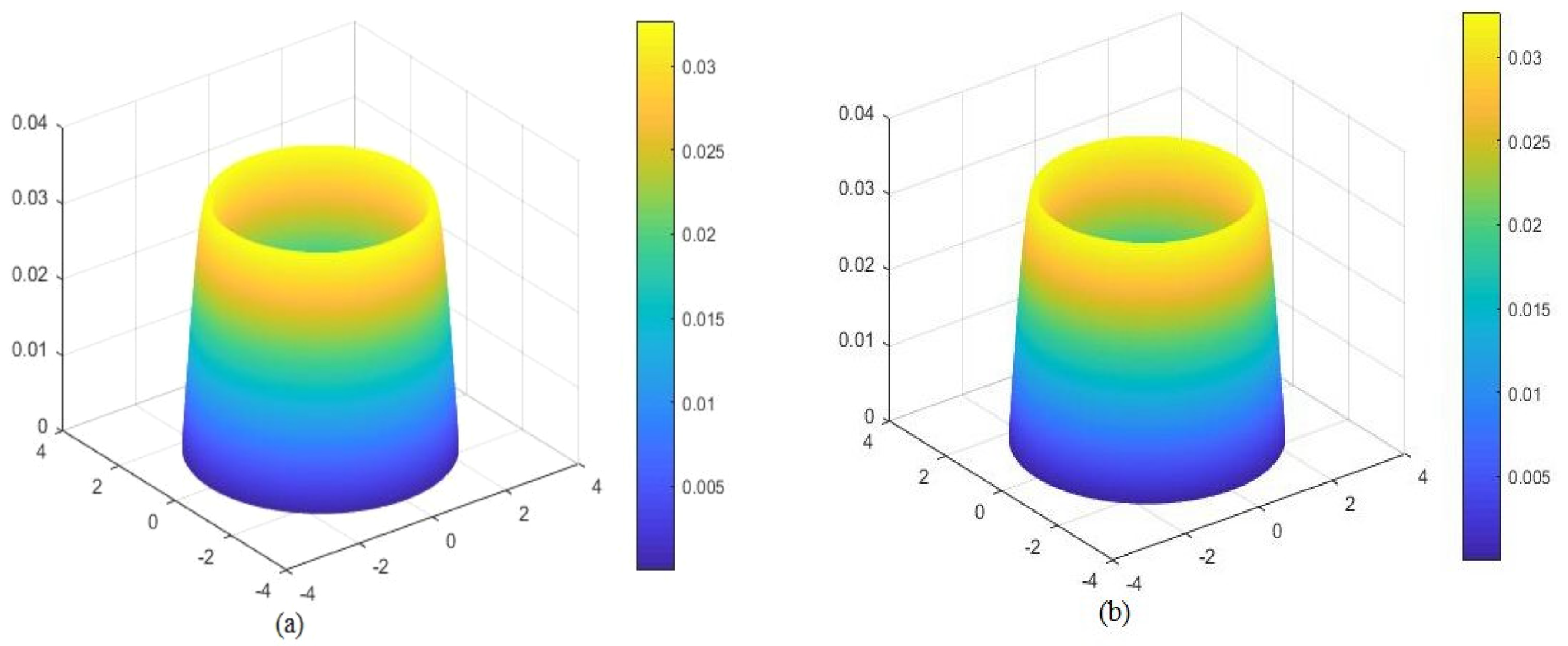
When $\alpha =\gamma =\beta =10$, we obtain the NBE solutions $u_h^k$ and the analytical solution $u(\mathit{z},t_k)$ at time $t=0.2$, $0.4$, $0.6$, $0.8$, $1.0,$ and $1.2$ and exhibit them in (a) and (b) of Figure 2, Figure 3, Figure 4, Figure 5, Figure 6 and Figure 7, respectively. From each pair of images in Figure 2, Figure 3, Figure 4, Figure 5, Figure 6 and Figure 7, we can clearly observe that the analytical solutions are basically the same as the NBE solutions.

Figure 2. (a) The NBE solution $u^k$ at $t=0.2$. (b) The analytical solution $u_h^k$ at $t=0.2$.

Figure 3. (a) The NBE solution $u^k$ at $t=0.4$. (b) The analytical solution $u_h^k$ at $t=0.4$.

Figure 4. (a) The NBE solution $u^k$ at $t=0.6$. (b) The analytical solution $u_h^k$ at $t=0.6$.

Figure 5. (a) The NBE solution $u^k$ at $t=0.8$. (b) The analytical solution $u_h^k$ at $t=0.8$.

Figure 6. (a) The NBE solution $u^k$ at $t=1$. (b) The analytical solution $u_h^k$ at $t=1$.

Figure 7. (a) The NBE solution $u^k$ at $t=1.2$. (b) The analytical solution $u_h^k$ at $t=1.2$.

4.2. The Second Numerical Example, Namely the Case at $\alpha =\gamma =\beta =100$

When $\alpha =\gamma =\beta =100$, we also obtain the NBE solutions $u_h^k$ and the analytical solution $u(\mathit{z},t_k)$ at time $t=0.2$, $0.4$, $0.6$, $0.8$, $1.0,$ and $1.2$ and exhibit them in (a) and (b) of Figure 8, Figure 9, Figure 10, Figure 11, Figure 12 and Figure 13, respectively. Comparing each pair of images in Figure 8, Figure 9, Figure 10, Figure 11, Figure 12 and Figure 13, we can also clearly observe that the NBE solutions are basically the same as the analytical solutions.

Figure 8. (a) The NBE solution $u^k$ at $t=0.2$. (b) The analytical solution $u_h^k$ at $t=0.2$.

Figure 9. (a) The NBE solution $u^k$ at $t=0.4$. (b) The analytical solution $u_h^k$ at $t=0.4$.

Figure 10. (a) The NBE solution $u^k$ at $t=0.6$. (b) The analytical solution $u_h^k$ at $t=0.6$.

Figure 11. (a) The NBE solution $u^k$ at $t=0.8$. (b) The analytical solution $u_h^k$ at $t=0.8$.

Figure 12. (a) The NBE solution $u^k$ at $t=1.0$. (b) The NBE solution $u_h^k$ at $t=1.0$.

Figure 13. (a) The NBE solution $u^k$ at $t=1.2$. (b) The analytical solution $u_h^k$ at $t=1.2$.

The $L^2$-norm errors between the NBE solutions $u_h^k$ and the analytical solution $u(\mathit{z},t_k)$ at $t=0.2$, $0.4$, $0.6$, $0.8$, $1.0$, and $1.2$ for the two cases are shown graphically in Figure 14. It has been certified that the numerical simulation results accord with the theory results since both errors reach $O\left({10}^{-4}\right)$. This sufficiently indicates that the NBE method is feasible and effective at finding the numerical solutions of the UTL equation defined in the 2D boundless region and is “robust”.

Figure 14. The $L^2$-norm errors between the analytical solutions and the NBE solutions at $t\in [0.2,1.2]$.

5. Conclusions

Herein, we created the time semi-discretized formulation of the UTL equation defined in the 2D boundless region and analyzed the errors of second-order convergence for the time semi-discretized solutions. Then, we established the fully discretized NBE formulation and discussed the errors between the fully discretized NBE solutions and the analytical solution. We also employed two numerical examples to show that the NBE method is feasible and effective. The most important of all is that the NBE method for solving the UTL equation defined in the 2D boundless region has been first proposed by us and is original and new. Besides, the method can be also used to settle many real-world issues, such as the Allen–Cahn equations [18] and the viscoelastic wave equation [19].