Dynamical Analysis of a One- and Two-Scroll Chaotic System

Abstract

In this paper, a three-dimensional (3D) autonomous chaotic system is introduced and analyzed. In the system, each equation contains a quadratic crossproduct. The system possesses a chaotic attractor with a large chaotic region. Importantly, the system can generate both one- and two-scroll chaotic attractors by choosing appropriate parameters. Some of its basic dynamical properties, such as the Lyapunov exponents, Lyapunov dimension, Poincaré maps, bifurcation diagram, and the chaotic dynamical behavior are studied by adjusting different parameters. Further, an equivalent electronic circuit for the proposed chaotic system is designed according to Kirchhoff’s Law, and a corresponding response electronic circuit is also designed for identifying the unknown parameters or monitoring the changes in the system parameters. Moreover, numerical simulations are presented to perform and complement the theoretical results.

1. Introduction

Since the first discovery of chaotic attractors by Lorenz in 1963 [1], chaos has attracted attention and interest for its useful speciality and application in information and computer science [2]. The proposals of new chaotic systems have been extensively studied by scientists in the past decades. In 1976, Rössler found a new simple 3D quadratic autonomous chaotic system with only one quadratic nonlinearity on the right-hand side [3].

In 1999, Chen found another chaotic attractor [4]. Recently, Lü and Chen further found a new chaotic system, which represented the transition between the Lorenz and the Chen system [5]. Moreover, Liu and Chen introduced a new chaotic system with three quadratic nonlinearities on the right-hand side in 2003 [6], which displayed two- and four-scroll attractors for different parameters. Then, Lü and Chen constructed another simple 3D system, which displayed two chaotic attractors simultaneously [7].

During the past few years, some new 3D chaotic systems have been analyzed [8,9,10,11,12,13,14,15,16,17,18,19,20]. To classify these 3D autonomous chaotic systems, Vaněček and Čelikoshý [21] gave a divertive classification by separating the linear and quadratic parts of a 3D autonomous system. The linear part was described by a constant matrix $A={\left[a_{ij}\right]}_{3\times 3}$. The Lorenz system satisfied $a_{12}{a}_{21}>0$, the Chen system satisfied $a_{12}{a}_{21}<0$, and the Lü system satisfied $a_{12}{a}_{21}=0$. As is known, the Lorenz system and Chen system display a two-scroll chaotic attractor separately. In this paper, we introduce a 3D autonomous system, in which each equation contains a quadratic crossproduct, and the constant matrix of the linear part satisfies $a_{12}{a}_{21}=0$. Different from Lorenz-like systems, the proposed system can display different numbers of scroll chaotic attractors simultaneously. The system is described by:

$$\left\{\begin{array}{c}\dot{x}=ay-yz,\hfill \\ \dot{y}=-bz+zx,\hfill \\ \dot{z}=cx+xy-dz,\hfill \end{array}\right.$$

(1)

in which ${(x,y,z)}^T\in {\Re }^3$, and $a,b,c,$ and d are real parameters. Though system (1) has three quadratic nonlinearities on the right-hand side, it can display only one-scroll attractor in contrast to the Rössler attractor and Sprott’s attractor [22,23]. Simultaneously, with the appropriate parameters, the system (1) can display a two-scroll attractor in contrast to the famous Lorenz attractor. This system is a supplement to the discovery of two-scroll band structure attractors.

Further, according to Kirchhoff’s law, we design an equivalent electronic circuit for the proposed chaotic system to show its practical applications. The system parameters of an electronic circuit maybe unknown or uncertain. Thus, based on the parameter identification and adaptive synchronization of drive–response systems, we design a corresponding response electronic circuit to identify the unknown parameters or monitor the changes in the system parameters.

The outline of this paper is as follows. In Section 2, the basic dynamical behavior in the parameter space is discussed, and some parameter examples for generating chaos are given. In Section 3, bifurcation analysis and the simulation results of the chaotic system are presented. In Section 4, a vector map is employed to generalized different attractors with the same parameters in the system. In Section 5, the adaptive synchronization problem between the drive–response systems with fully unknown parameters is studied. Finally, conclusions are drawn in Section 6.

2. Basic Dynamical Behavior of the System

The divergence of system (1) is

$$\nabla \dot{V}=\frac{\partial \dot{x}}{\partial x}+\frac{\partial \dot{y}}{\partial y}+\frac{\partial \dot{z}}{\partial z}=0+0-d=-d.$$

(2)

Therefore, when parameter d is positive, system (1) is dissipative.

The equilibria of system (1) can be obtained by solving the following algebraic equations:

$$ay-yz=0,-bz+xz=0,cx+xy-dz=0.$$

When $bd\ne 0$, the system has three equilibria:

$$S_1={(0,0,0)}^T,S_2={(b,\frac{ad-bc}{b},a)}^T,S_3={(b,0,\frac{bc}{d})}^T.$$

In addition, under the condition $b=0$ (or $d=0$), the system has a unique equilibrium $S_{01}^{\ast }={(0,0,0)}^T$ (or $S_{02}^{\ast }={(b,-c,a)}^T$). In the following, we let $b\ne 0$ and $d>0$. The Jacobian matrix of system (1) at the three equilibria $S_1$, $S_2$, and $S_3$ are

$$J_1=\left(\begin{array}{ccc}0& a& 0\\ 0& 0& -b\\ c& 0& -d\end{array}\right),J_2=\left(\begin{array}{ccc}0& 0& \frac{bc-ad}{b}\\ a& 0& 0\\ \frac{ad}{b}& b& -d\end{array}\right),$$

$$J_3=\left(\begin{array}{ccc}0& \frac{ad-bc}{d}& 0\\ \frac{bc}{d}& 0& 0\\ c& b& -d\end{array}\right).$$

The characteristic equations of $J_1$, $J_2$, and $J_3$ are

$${\lambda }^3+d{\lambda }^2+abc=0,$$

(3)

$${\lambda }^3+d{\lambda }^2+\frac{a^2{d}^2-abcd}{b^2}\lambda +a^{2}d-abc=0,$$

(4)

$$(\lambda +d)({\lambda }^2+\frac{b^2{c}^2-abcd}{d^2})=0.$$

(5)

Obviously, from Equation (5), the equilibrium $S_3$ is a saddle for $bc(bc-ad)<0$ and is a center for $bc(bc-ad)>0$.

According to the Routh–Hurwitz criterion [24,25], for a cubic characteristic equation

$${\lambda }^3+a_1{\lambda }^2+a_2\lambda +a_3=0,$$

(6)

the real part of the roots of the cubic Equation (6) is negative if and only if $a_1>0$, $a_3>0$, $a_1{a}_2-a_3>0$, i.e., (6) satisfies the condition $\left|arg\right(\lambda \left)\right|>\pi /2$. Then, the equilibrium point of system (1) is locally asymptotically stable.

Comparing Equation (3) with Equation (6), it is impossible to satisfy the conditions $abc>0$ and $-abc>0$ simultaneously, i.e., when $abc>0$ (or $abc<0$) and $d>0$, the equilibrium $S_1$ is unstable. For instance, when $a=0.4$, $b=60$, $c=16$, and $d=10$, the three eigenvalues corresponding to $S_1=(0,0,0)$ are ${\lambda }_1=-12.4696$ and ${\lambda }_{2,3}=1.2348\pm 5.4102i$, and the system has a chaotic attractor at the unstable equilibrium $S_1$ for the initial value ${(0.01,0.01,0.01)}^T$ as shown in Figure 1.

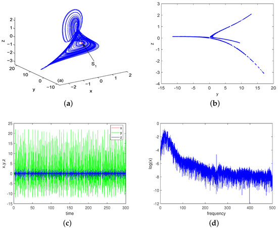
Figure 1. (a) Chaotic attractor of system (1) with $(a,b,c,d)=(0.4,60,16,10)$ at the initial values ${(0.01,0.01,0.01)}^T$. (b) The corresponding Poincaré map on plane $x=0$. (c) The time series of the $x,y,z$ states. (d) The power spectrum of the x state.

Similarly, comparing Equation (4) with Equation (6), when one or two of the three conditions (i.e., $a(ad-bc)>0$, $d^2-b^2>0$, and $d>0$) are not satisfied, the equilibrium $S_2$ is unstable, and system (1) can generate chaos at $S_1$ and $S_2$. For instance, when $a=5$, $b=50$, $c=-6$, and $d=13$, the three eigenvalues corresponding to $S_2={(50,7.3,5)}^T$ are ${\lambda }_1=-18.0662$ and ${\lambda }_{2,3}=2.5331\pm 9.7263i$, and the three eigenvalues corresponding to $S_3={(50,0,-23.0769)}^T$ are ${\lambda }_1=-13$ and ${\lambda }_{2,3}=\pm 25.4544i$. The system has a chaotic attractor at unstable equilibrium $S_2$, as shown in Figure 2.

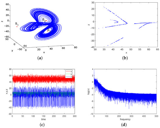
Figure 2. (a) Chaotic attractor of system (1) with $(a,b,c,d)=(5,50,-6,13)$ at the initial values ${(50.01,7.31,5.01)}^T$. (b) The corresponding Poincaré map on plane $y=5$. (c) The time series of the $x,y,z$ states. (d) The power spectrum of the x state.

3. Bifurcation Analysis

As is known, for a 3D autonomous system, its three Lyapunov exponents $L_1$, $L_2$, and $L_3$ can be obtained by using the Wolf algorithm [26]. For the equilibrium points, $L_3<L_2<L_1<0$, for the periodic orbits, $L_3<L_2<0$, $L_1=0$, and for the chaotic attractor, $L_3<0,L_2=0$, $L_1>0$. In the following, the Lyapunov exponent spectrum and the corresponding bifurcation diagram of state variable x with respect to different parameters are shown, and the basic dynamics of the chaotic system (1) are summarized as follows. In addition, the Lyapunov exponents $L_i$ and the Lyapunov dimension $D_L$ are listed, in which the Lyapunov dimension of chaos attractors is a fractional dimension, described as:

$$D_L=j+\frac{1}{\mid L_{j+1}\mid }\sum _{i=1}^j{L}_i=2+\frac{L_1+L_2}{\mid L_3\mid }.$$

(7)

In this section, system (1) is investigated under the condition that the four parameters are all positive, as shown in Table 1. Some examples according to different conditions of the parameters are shown in Table 1 and Table 2, which cause system (1) to display chaotic attractors at $S_1$ and $S_2$, respectively.

Table 1. Parameter examples and Lyapunov exponents for chaotic system (1) that generate chaos at the equilibrium $S_1$.

$\mathbf{abc}>0$ and $\mathit{d}>0$	Parameter Examples	Lyapunov Exponents	${\mathit{D}}_{\mathit{L}}$	Initial Values
	$a=0.3,b=60,c=16,d=10$	$L_1=0.422,L_2=0,L_3=-10.419$	2.0404	${(0.01,0.01,0.01)}^T$
$a>0,b>0,c>0$,	$a=0.45,b=62,c=16.1,d=9$	$L_1=0.883,L_2=0,L_3=-9.883$	2.0897	${(0.01,0.01,0.01)}^T$
	$a=1.2,b=18,c=15,d=8$	$L_1=0.776,L_2=0,L_3=-8.775$	2.0885	${(0.01,0.01,0.01)}^T$
	$a=0.85,b=-20,c=-16,d=10$	$L_1=0.314,L_2=0,L_3=-10.314$	2.0306	${(0.01,0.01,0.01)}^T$
$a>0,b<0,c<0$,	$a=0.85,b=-30,c=-19,d=1$	$L_1=0.895,L_2=0,L_3=-10.891$	2.0821	${(0.01,0.01,0.01)}^T$
	$a=0.65,b=-30,c=-16,d=10$	$L_1=0.443,L_2=0,L_3=-10.441$	2.0424	${(0.01,0.01,0.01)}^T$
	$a=-2,b=-21,c=16,d=10$	$L_1=1.022,L_2=0,L_3=-11.020$	2.0931	${(0.01,0.01,0.01)}^T$
$a<0,b<0,c>0$,	$a=-2,b=-15,c=16,d=9$	$L_1=0.881,L_2=0,L_3=-9.882$	2.0896	${(0.01,0.01,0.01)}^T$
	$a=-10,b=-8,c=9,d=8$	$L_1=1.115,L_2=0,L_3=-9.115$	2.1236	${(0.01,0.01,0.01)}^T$
	$a=-1,b=40,c=-18,d=12$	$L_1=0.924,L_2=0,L_3=-12.918$	2.0715	${(0.01,0.01,0.01)}^T$
$a<0,b>0,c<0$,	$a=-0.7,b=30,c=-16,d=10$	$L_1=0.570,L_2=0,L_3=-10.568$	2.0539	${(0.01,0.01,0.01)}^T$
	$a=-1.2,b=20,c=-16,d=9$	$L_1=0.743,L_2=0,L_3=-9.742$	2.0763	${(0.01,0.01,0.01)}^T$

Table 2. Parameter examples and Lyapunov exponents for chaotic system (1) that generate chaos at the equilibrium $S_1$.

$\mathbf{abc}<0$ and $\mathit{d}>0$	Parameter Examples	Lyapunov Exponents	${\mathit{D}}_{\mathit{L}}$	Initial Values
$a(ad-bc)>0,$	$a=5,b=50,c=-6,d=13$	$L_1=1.283,L_2=0,L_3=-14.261$	2.0906	${(50.01,7.31,5.01)}^T$
$d^2-b^2<0,b>0$	$a=12,b=50,c=-6.1,d=13$	$L_1=1.586,L_2=0,L_3=-14.574$	2.1093	${(50.01,7.31,5.01)}^T$
	$a=-16,b=60,c=3,d=9$	$L_1=1.328,L_2=0,L_3=-10.328$	2.1290	${(50.01,7.31,5.01)}^T$
$a(ad-bc)>0,$	$a=16,b=-60,c=3,d=9$	$L_1=1.365,L_2=0,L_3=-10.367$	2.1277	${(-50.01,7.31,5.01)}^T$
$d^2-b^2<0,b<0$	$a=10,b=-50,c=3,d=10$	$L_1=1.376,L_2=0,L_3=-11.366$	2.1212	${(-50.01,7.31,5.01)}^T$
	$a=20,b=-70,c=3,d=10$	$L_1=1.383,L_2=0,L_3=-11.379$	2.1216	${(-50.01,7.31,5.01)}^T$

We fixed $b=60$, $c=16$, and $d=10$, and the Lyapunov exponent spectrum with respect to a is shown in Figure 3. When the parameter a varied in the small interval $(0,0.66)$, system (1) had very rich dynamical behaviors, i.e., when $a\in (0,0.171)\cup (0.219,0.231)\cup (0.257,0.269)\cup (0.473,0.526)$, the maximum Lyapunov exponent equaled zero, and system (1) had periodic orbits, and when $a\in (0.171,0.219)\cup (0.231,0.257)\cup (0.269,0.473)\cup (0.526,0.66)$, there was one positive Lyapunov exponent, and system (1) was chaotic.

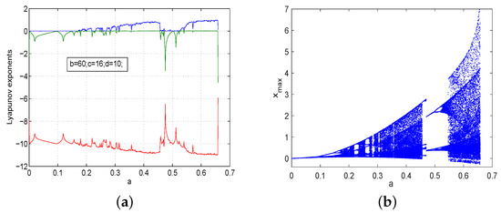
Figure 3. The Lyapunov exponents spectrum and the bifurcation diagram of system (1) with $(b,c,d)=(60,16,10)$ and $0<a<0.66$ at the initial values ${(0.01,0.01,0.01)}^T$: (a) Lyapunov exponents; (b) bifurcation diagram.

We fixed a, c, and d, and the Lyapunov exponent spectrum with respect to b is shown in Figure 4 and Figure 5. We fixed $a=0.4,c=16,$ and $d=10$; when b varied in the interval $(0,97)$, system (1) had very rich dynamical behaviors at the initial values ${(0.01,0.01,0.01)}^T$, i.e., when $b\in (0,25.7)\cup (29.3,30.2)\cup (32.9,35)\cup (39.3,41)\cup (68.5,78.5)$, the maximum Lyapunov exponent equaled zero, and system (1) had periodic orbits, and when $b\in (25.7,29.3)\cup (30.2,32.9)\cup (35,39.3)\cup (41,68.5)\cup (78.5,97)$, there was one positive Lyapunov exponent, and system (1) was chaotic. On the other hand, we fixed $a=5,c=-6,$ and $d=13$; when b varied in the interval $(45,60)$, system (1) had very rich dynamical behaviors at the initial values ${(50.01,7.31,5.01)}^T$ as well, i.e., when $b\in (45.6,46.9)\cup (50.3,50.5)\cup (54.6,55.2)$, the maximum Lyapunov exponent equaled zero, and system (1) had periodic orbits, and when $b\in (45,45.6)\cup (46.9,50.3)\cup (50.5,54.6)\cup (55.2,56.82)$, there was one positive Lyapunov exponent, and system (1) was chaotic.

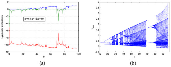
Figure 4. The Lyapunov exponents spectrum and the bifurcation diagram of system (1) with $(a,c,d)=(0.4,16,10)$ and $0<b<97$ at the initial values ${(0.01,0.01,0.01)}^T$: (a) Lyapunov exponents; (b) bifurcation diagram.

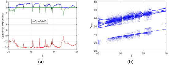
Figure 5. The Lyapunov exponents spectrum and the bifurcation diagram of system (1) with $(a,c,d)=(5,-6,13)$ and $45<b<60$ at the initial values ${(50.01,7.31,5.01)}^T$: (a) Lyapunov exponents; (b) bifurcation diagram.

We fixed $a=0.4,b=60,$ and $d=10$; when c varied in the interval $(2.7,20.2)$, system (1) had very rich dynamical behaviors, i.e., when $c\in (2.7,9.1)\cup (10.12,10.21)\cup (11.7,12.1)\cup (17.38,17.77)$, the maximum Lyapunov exponent equaled zero, and system (1) had periodic orbits, and when $c\in (9.1,10.12)\cup (10.21,11.7)\cup (12.1,17.38)\cup (17.77,20.2)$, there was one positive Lyapunov exponent, and system (1) was chaotic. The corresponding Lyapunov exponent and bifurcation diagram are shown in Figure 6.

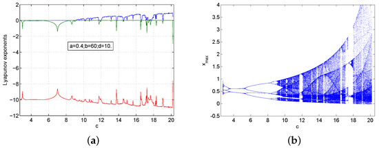
Figure 6. The Lyapunov exponents spectrum and the bifurcation diagram of system (1) with $(a,b,d)=(0.4,60,10)$ and $2.7<c<20.2$ at the initial values ${(0.01,0.01,0.01)}^T$: (a) Lyapunov exponents; (b) bifurcation diagram.

We fixed $a=0.4,b=60,$ and $c=16$; when d varied in the interval $(8.49,20)$, system (1) had very rich dynamical behaviors at the initial values ${(0.01,0.01,0.01)}^T$, i.e., when $d\in (9.35,9.65)\cup (11.58,20)$, the maximum Lyapunov exponent equaled zero, and system (1) had periodic orbits, and when $d\in (8.49,9.35)\cup (9.65,11.58)$, there was one positive Lyapunov exponent. and system (1) was chaotic. The corresponding Lyapunov exponent and bifurcation diagram are shown in Figure 7 and Figure 8. On the other hand, we fixed $a=5,b=50,$ and $c=-6$; when d varied in the interval $(5,30)$, system (1) had very rich dynamical behaviors at the initial values ${(50.01,7.31,5.01)}^T$ as well, i.e., when $b\in (5,5.4)\cup (11.9,12.2)\cup (13.3,13.6)\cup (13.8,14.1)\cup (14.8,15.1)\cup (16.6,16.8)\cup (17.8,23.1)\cup (24.9,30)$, the maximum Lyapunov exponent equaled zero, and system (1) had periodic orbits, and when $b\in (5.4,11.9)\cup (12.2,13.3)\cup (13.6,13.8)\cup (14.1,14.9)$ $\cup (15.1,16.6)\cup (16.8,17.8)\cup (23.1,24.9)$, there was one positive Lyapunov exponent, and system (1) was chaotic.

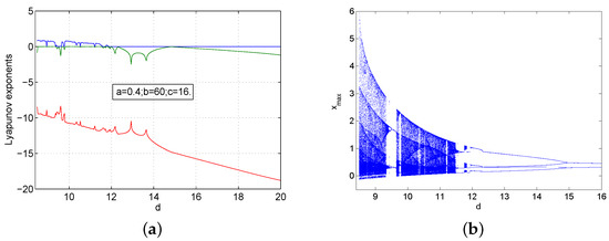
Figure 7. The Lyapunov exponents spectrum and the bifurcation diagram of system (1) with $(a,b,c)=(0.4,60,16)$ and $8.49<d<20$ at the initial values ${(0.01,0.01,0.01)}^T$: (a) Lyapunov exponents; (b) bifurcation diagram.

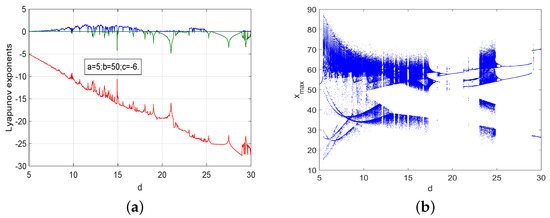
Figure 8. The Lyapunov exponents spectrum and the bifurcation diagram of system (1) with $(a,b,c)=(5,50,-6)$ and $5<d<30$ at the initial values ${(50.01,7.31,5.01)}^T$: (a) Lyapunov exponents; (b) bifurcation diagram.

In Figure 9, some simulation results of system (1) with different parameter values are given in the $x-y-z$ space.

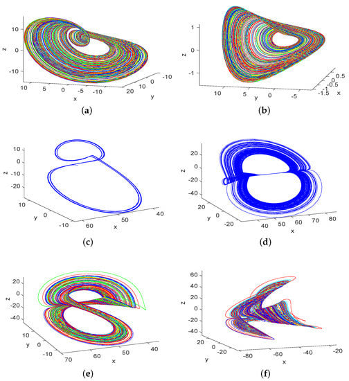
Figure 9. The phase portrait of system (1) with different parameter values: (a) $a=5.8,b=9,c=15,d=11$; (b) $a=0.4,b=60,c=10,d=10$; (c) $a=5,b=50,c=-6,d=25.5$; (d) $a=5,b=60,c=-6,d=34$; (e) $a=5,b=55,c=-6,d=16$; (f) $a=16,b=-60,c=3,d=9$.

4. Chaotic Systems Generalized by a Vector Map

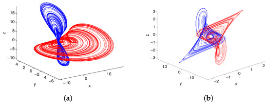
In this section, we introduce several chaotic systems generalized by a vector map. Firstly, system (1) can be written as:

$$\left(\begin{array}{c}\dot{x}\\ \dot{y}\\ \dot{z}\end{array}\right)=\left(\begin{array}{ccc}0& y& 0\\ 0& 0& z\\ x& 0& 0\end{array}\right)A+\left(\begin{array}{ccc}x& 0& 0\\ 0& y& 0\\ 0& 0& z\end{array}\right)B+\left(\begin{array}{ccc}yz& 0& 0\\ 0& xz& 0\\ 0& 0& xy\end{array}\right)C,$$

(8)

where $A={(c,a,-b)}^T$, $B={(0,0,-d)}^T$, and $C={(-1,1,1)}^T$ are the parameter vectors. Now, we define the following vector maps ${\varphi }_i:{\Re }^3\to {\Re }^3,i=1,2:$

$$\begin{array}{c}\hfill {\varphi }_1\left({(x_1,x_2,x_3)}^T\right)={(x_2,x_3,x_1)}^T,\\ \hfill {\varphi }_2\left({(x_1,x_2,x_3)}^T\right)={(x_3,x_1,x_2)}^T.\end{array}$$

(9)

Then, system (10) is chaotic for the same parameters as (8):

$$\begin{array}{c}\hfill \left(\begin{array}{c}\dot{x}\\ \dot{y}\\ \dot{z}\end{array}\right)=\left(\begin{array}{ccc}0& y& 0\\ 0& 0& z\\ x& 0& 0\end{array}\right){\varphi }_i\left(A\right)+\left(\begin{array}{ccc}x& 0& 0\\ 0& y& 0\\ 0& 0& z\end{array}\right){\varphi }_i\left(B\right)\\ \hfill +\left(\begin{array}{ccc}yz& 0& 0\\ 0& xz& 0\\ 0& 0& xy\end{array}\right){\varphi }_i\left(C\right).\end{array}$$

(10)

Substituting Equation (9) into (10) yields two chaotic systems (11) and (12) with $a=1,b=22,c=16$, and $d=10$ and the initial value ${(0.1,0.1,0.1)}^T$. The two chaotic attractors are shown in Figure 10a.

$$\left\{\begin{array}{c}\dot{x}=-by+yz,\hfill \\ \dot{y}=cz+zx-dy,\hfill \\ \dot{z}=ax-xy,\hfill \end{array}\right.$$

(11)

$$\left\{\begin{array}{c}\dot{x}=cy+yz-dx,\hfill \\ \dot{y}=az-zx,\hfill \\ \dot{z}=-bx+xy.\hfill \end{array}\right.$$

(12)

Figure 10. (a) The red plot corresponds to system (11), and the blue plot corresponds to system (12), with (a,b,c,d)=(1,22,16,10). (b) The red plot corresponds to system (13), and the blue plot corresponds to system (1), with $(a,b,c,d)=(0.4,50,16,10)$.

In addition, if we only revise $C={(1,-1,-1)}^T$ in system (8), system (13) is chaotic for the same parameters as system (1), when we have the parameters $a=0.4,b=50,c=16$, and $d=10$ and the initial value ${(0.1,0.1,0.1)}^T$. The two chaotic attractors are shown in Figure 10b.

$$\left\{\begin{array}{c}\dot{x}=ay+yz,\hfill \\ \dot{y}=-bz-xz,\hfill \\ \dot{z}=cx-xy-dz.\hfill \end{array}\right.$$

(13)

5. Electronic Circuit Design

In this section, we present an equivalent electronic circuit for the proposed chaotic system (1). The circuit implementation shows that it can be practically used in technological applications. In order to implement the equations, we considered the analog circuit design using Multisim software, as depicted in Figure 11, with AD712KN operational amplifiers and AD633 analog multipliers all powered by $\pm 15$ V symmetric voltages.

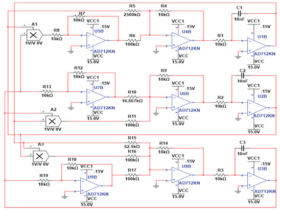
Figure 11. Electronic circuit schematics of the chaotic system (1).

Using the Kirchhoff Law for the analog circuit, the generated nonlinear equations are described as

$$\left\{\begin{array}{c}\dot{x}=\frac{R_4}{R_1{R}_5{C}_1}y+\frac{R_4{R}_7}{R_1{R}_6{R}_8{C}_1}yz,\hfill \\ \dot{y}=-\frac{R_9{R}_{12}}{R_2{R}_{10}{R}_{13}{C}_2}z+\frac{R_9}{R_2{R}_{11}{C}_2}zx,\hfill \\ \dot{z}=\frac{R_{14}}{R_3{R}_{15}{C}_3}x+\frac{R_{14}}{R_3{R}_{16}{C}_3}xy-\frac{R_{14}{R}_{18}}{R_3{R}_{17}{C}_3}z.\hfill \end{array}\right.$$

(14)

Comparing Equation (14) with Equation (1), the common circuital component values were selected as $C_1=C_2=C_3=10$ nF, $R_i=10$ k$\mathrm{\Omega }$ $(i=1,2,3,4,9,14)$, $R_i=100$ k$\mathrm{\Omega }$ $(i=6,11,16)$, and $R_i=10$ k$\mathrm{\Omega }$ $(i=7,8,12,13,18,19)$. When we chose $R_5=2500$ k$\mathrm{\Omega }$, $R_{10}=16.67$ k$\mathrm{\Omega }$, $R_{15}=62.5$ k$\mathrm{\Omega }$, and $R_{17}=100$ k$\mathrm{\Omega }$, we obtained a one-scoll chaotic attractor similar to the one obtained by numerical simulation with $(a,b,c,d)=(0.4,60,16,10)$, and the Multisim results on oscilloscope are shown as Figure 12a,b. When we chose $R_5=200$ k$\mathrm{\Omega }$, $R_{10}=20$ k$\mathrm{\Omega }$, $R_{15}=166.67$ k$\mathrm{\Omega }$, and $R_{17}=76.92$ k$\mathrm{\Omega }$, and modified the connection $R_{15}$ to $R_1$, we obtained a two-scoll chaotic attractor similar to the one obtained by numerical simulation with $(a,b,c,d)=(5,50,-6,13)$, and the Multisim results on the oscilloscope are shown as Figure 12c,d.

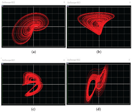
Figure 12. Phase spaces of the chaotic system (1) on an oscilloscope obtained from the analog circuit: (a) x-z; (b) y-z; (c) x-z; (d) y-z.

6. Parameter Identification

In this section, we supposed that the parameters $a,b,c,$ and$d$ of system (1) were unknown and needed to be identified. We regarded system (1) as the drive system. The response system with adaptive controllers and updating laws was designed as:

$$\left\{\begin{array}{c}\dot{x_1}=a_1{y}_1-y_1{z}_1+u_1,\hfill \\ \dot{y_1}=-b_1{z}_1+z_1{x}_1+u_2,\hfill \\ \dot{z_1}=c_1{x}_1+x_1{y}_1-d_1{z}_1+u_3,\hfill \end{array}\right.$$

(15)

where $a_1,b_1,c_1,$ and$d_1$ were the estimations of $a,b,c,$ and$d$, and $u_1,u_2,$ and$u_3$ were controllers to be designed.

Theorem 1. 

If we design the controllers $u_1,u_2,$ and$u_3$ in (15) as

$$\left\{\begin{array}{c}{u}_1=-k_1{e}_x,\hfill \\ u_2=-k_2{e}_y-x_1{e}_z,\hfill \\ u_3=-k_3{e}_z-x{e}_y,\hfill \\ {\dot{k}}_1={\alpha }_1{e}_x^2,\hfill \\ {\dot{k}}_2={\alpha }_2{e}_y^2,\hfill \\ {\dot{k}}_3={\alpha }_3{e}_z^2,\hfill \end{array}\right.$$

(16)

where ${\alpha }_1,{\alpha }_2,$ and${\alpha }_3$ are positive constants, and the updating laws of $a_1,b_1,c_1,$ and$d_1$ as

$$\left\{\begin{array}{c}{\dot{a}}_1=-{\theta }_1{y}_1{e}_x,\hfill \\ {\dot{b}}_1={\theta }_2{z}_1{e}_y,\hfill \\ {\dot{c}}_1=-{\theta }_3{x}_1{e}_z,\hfill \\ {\dot{d}}_1={\theta }_4{z}_1{e}_z,\hfill \end{array}\right.$$

(17)

where ${\theta }_1,{\theta }_2,{\theta }_3,$ and${\theta }_4$ are positive constants, then the adaptive synchronization between the drive–response systems (1) and (15) is achieved, and the unknown parameters $a,b,c,$ and$d$ in (1) are identified by $a_1,b_1,c_1,$ and$d_1$ in (15), with controllers (16) and updating laws (17).

Proof. 

Let $e_x=x_1-x,e_y=y_1-y,$ and $e_z=z_1-z$; then, one has

$$\left\{\begin{array}{c}\dot{e_x}=(a_1-a)y_1+a{e}_y-y_1{e}_z-e_{y}z+u_1,\hfill \\ \dot{e_y}=-(b_1-b)z_1-b{e}_z+x_1{e}_z+e_{x}z+u_2,\hfill \\ \dot{e_z}=(c_1-c)x_1+c{e}_x+e_x{y}_1+x{e}_y-(d_1-d)z_1-d{e}_z+u_3.\hfill \end{array}\right.$$

(18)

We consider the following Lyapunov function

$$\begin{array}{cc}\hfill V\left(t\right)=& \frac{e_x^2+e_y^2+e_z^2}{2}+\frac{{(a_1-a)}^2}{2{\theta }_1}+\frac{{(b_1-b)}^2}{2{\theta }_2}\hfill \\ \hfill & +\frac{{(c_1-c)}^2}{2{\theta }_3}+\frac{{(d_1-d)}^2}{2{\theta }_4}+\sum _{i=1}^3\frac{{(k_i-k_i^{\ast })}^2}{2{\alpha }_i},\hfill \end{array}$$

(19)

where $k_1^{\ast },k_2^{\ast },$ and $k_3^{\ast }$ are arbitrary positive constants to be determined.

Then, the derivative of $V\left(t\right)$ along the trajectories of (18) gives

$$\begin{array}{cc}\hfill \dot{V}\left(t\right)=& e_x{\dot{e}}_x+e_y{\dot{e}}_y+e_z{\dot{e}}_z+\frac{(a_1-a){\dot{a}}_1}{{\theta }_1}+\frac{(b_1-b){\dot{b}}_1}{{\theta }_2}\hfill \\ \hfill & +\frac{(c_1-c){\dot{c}}_1}{{\theta }_3}+\frac{(d_1-d){\dot{d}}_1}{{\theta }_4}+\sum _{i=1}^3\frac{(k_i-k_i^{\ast }){\dot{k}}_i}{{\alpha }_i}\hfill \\ \hfill =& e^T(P-K)e,\hfill \end{array}$$

where $e={(e_x,e_y,e_z)}^T$,

$$P=\left(\begin{array}{ccc}0& \frac{a}{2}& \frac{c}{2}\\ \frac{a}{2}& 0& -\frac{b}{2}\\ \frac{c}{2}& -\frac{b}{2}& -d\end{array}\right),K=\left(\begin{array}{ccc}{k}_1^{\ast }& 0& 0\\ 0& k_2^{\ast }& 0\\ 0& 0& k_3^{\ast }\end{array}\right).$$

Then, one can choose $k_1^{\ast },k_2^{\ast },$ and $k_3^{\ast }$ large enough such that $P-K<0$, i.e., $\dot{V}\left(t\right)<0$, which implies that the adaptive synchronization is achieved, and the unknown parameters $a,b,c,$ and$d$ are identified by $a_1,b_1,c_1,$ and$d_1$. Thus, the proof is complete. □

In the simulations, we designed the corresponding electronic circuit with controllers (16) and updating laws (17) to identify the unknown parameters using Multisim software. Figure 13 shows the electronic circuit design with the AD712KN operational amplifiers and AD633 analog multipliers all powered by $\pm 15$ V symmetric voltages. We supposed that the resistances $R_{22},R_{12},R_{14},$ and $R_{17}$ of the drive system corresponding to the parameters $a=0.4,b=60,c=16,$ and$d=10$ of system (1) were unknown and needed to be identified. We chose the following resistances of the updating laws $R_a=R_b=R_c=R_d=50$ k$\mathrm{\Omega }$ and the following resistances of the controllers $R_{K_1}=R_{K_2}=R_{K_3}=100$ k$\mathrm{\Omega }$. The Multisim results on the oscilloscope are shown as Figure 14a,b. Clearly, the unknown parameters $a,b,c,$ and$d$ were well identified by $a_1,b_1,c_1,$ and$d_1$.

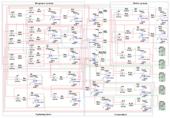
Figure 13. Electronic circuit schematics of the parameter identification.

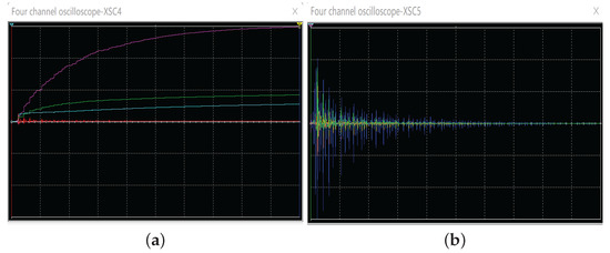
Figure 14. Identification of $a_1,b_1,c_1,$ and $d_1$ by an electronic circuit.

7. Conclusions

In this paper, we introduced and studied a new 3D autonomous chaotic system, which could generate one-scroll and two-scroll chaotic attractors with different parameters. The dynamical behaviors and properties of this chaotic system were investigated both theoretically and numerically. The Lyapunov exponent spectrum and the corresponding bifurcation diagram, with respect to different parameters, were presented, and these validated the correctness of our results. Spectral analysis showed that the system had a large chaos region. Moreover, a vector map was employed to the generalized chaotic system. Compared with the famous Rössler, Sprott, and Lorenz attractors, this system is a supplement to the discovery of one-scroll and two-scroll attractors. Further, we designed an equivalent electronic circuit for the proposed chaotic system based on Kirchhoff’s Law to show its practical applications. We designed a corresponding response electronic circuit to identify the unknown parameters or monitor the changes in the system parameters as well. Finally, numerical simulations were presented to perform and complement the theoretical results.

References

- Lorenz, E.N. Deterministic Nonperiodic Flow. J. Atmos. Sci. 1963, 20, 130–141. [Google Scholar] [CrossRef]
- Fallahi, K.; Leung, H. A chaos secure communication scheme based on multiplication modulation. Commun. Nonlinear Sci. Numer. Simul. 2010, 15, 368–383. [Google Scholar] [CrossRef]
- Rössler, O.E. An equation for continuous chaos. Phys. Lett. A 1976, 57, 397–398. [Google Scholar] [CrossRef]
- Chen, G.; Ueta, T. Yet another chaotic attractor. Int. J. Bifurc. Chaos 1999, 9, 1465–1466. [Google Scholar] [CrossRef]
- Lü, J.; Chen, G.; Cheng, D.; Celikovsky, S. Bridge the gap between the Lorenz system and the Chen system. Int. J. Bifurc. Chaos Appl. Sci. Eng. 2002, 12, 2917–2926. [Google Scholar] [CrossRef]
- Liu, W.; Chen, G. A new chaotic system and its generation. Int. J. Bifurc. Chaos Appl. Sci. Eng. 2003, 13, 261–267. [Google Scholar] [CrossRef]
- Lü, J.; Chen, G.; Cheng, D. A New Chaotic System and Beyond: The Generalized Lorenz-like System. Int. J. Bifurc. Chaos 2004, 14, 1507–1537. [Google Scholar] [CrossRef]
- Dong, G.; Du, R.; Tian, L.; Jia, Q. A novel 3D autonomous system with different multilayer chaotic attractors. Phys. Lett. Sect. A: Gen. At. Solid State Phys. 2009, 373, 3838–3845. [Google Scholar] [CrossRef]
- Wang, Z.; Qi, G.; Sun, Y.; Van Wyk, B.J.; Van Wyk, M.A. A new type of four-wing chaotic attractors in 3-D quadratic autonomous systems. Nonlinear Dyn. 2010, 60, 443–457. [Google Scholar] [CrossRef][Green Version]
- Wei, Z.; Yang, Q. Dynamical analysis of a new autonomous 3-D chaotic system only with stable equilibria. Nonlinear Anal. Real World Appl. 2011, 12, 106–118. [Google Scholar] [CrossRef]
- Liu, Y. Analysis of global dynamics in an unusual 3D chaotic system. Nonlinear Dyn. 2012, 70, 2203–2212. [Google Scholar] [CrossRef]
- Wang, X.; Chen, G. Constructing a chaotic system with any number of equilibria. Nonlinear Dyn. 2013, 71, 429–436. [Google Scholar] [CrossRef]
- Li, C.; Sprott, J.C.; Xing, H. Constructing chaotic systems with conditional symmetry. Nonlinear Dyn. 2017, 87, 1351–1358. [Google Scholar] [CrossRef]
- Wang, G.; Yuan, F.; Chen, G.; Zhang, Y. Coexisting multiple attractors and riddled basins of a memristive system. Chaos 2018, 28, 013125. [Google Scholar] [CrossRef]
- Zhang, X.; Wang, C.; Yao, W.; Lin, H. Chaotic system with bondorbital attractors. Nonlinear Dyn. 2019, 97, 2159–2174. [Google Scholar] [CrossRef]
- Xie, Q.; Zeng, Y. Generating different types of multi-double-scroll and multi-double-wing hidden attractors. Eur. Phys. J. Spec. Top. 2020, 229, 1361–1371. [Google Scholar] [CrossRef]
- Gong, L.; Wu, R.; Zhou, N. A New 4D Chaotic System with Coexisting Hidden Chaotic Attractors. Int. J. Bifurc. Chaos 2020, 30, 2050142. [Google Scholar] [CrossRef]
- Zhou, L.; You, Z.; Tang, Y. A new chaotic system with nested coexisting multiple attractors and riddled basins. Chaos Solitons Fractals 2021, 148, 111057. [Google Scholar] [CrossRef]
- Ma, C.; Mou, J.; Xiong, L.; Banerjee, S.; Liu, T.; Han, X. Dynamical analysis of a new chaotic system: Asymmetric multistability, offset boosting control and circuit realization. Nonlinear Dyn. 2021, 103, 2867–2880. [Google Scholar] [CrossRef]
- Wang, R.; Li, C.; Kong, S.; Jiang, Y.; Lei, T. A 3D memristive chaotic system with conditional symmetry. Chaos Soliton Fractal 2022, 158, 111992. [Google Scholar] [CrossRef]
- Vanecek, A.; Celikoshy, S. Control Systems: From Linear Analysis to Synthesis of Chaos; Prentice-Hall: London, UK, 1996. [Google Scholar]
- Sprott, J.C. Some simple chaotic flows. Phys. Rev. E 1994, 50, R647–R650. [Google Scholar] [CrossRef] [PubMed]
- Sprott, J.C. Simplest dissipative chaotic flow. Phys. Lett. Sect. A: Gen. At. Solid State Phys. 1997, 228, 271–274. [Google Scholar] [CrossRef]
- Huang, K.; Yang, Q. Stability and Hopf bifurcation analysis of a new system. Chaos Solitons Fractals 2009, 39, 567–578. [Google Scholar] [CrossRef]
- Zheng, S.; Dong, G.; Bi, Q. A new hyperchaotic system and its synchronization. Appl. Math. Comput. 2010, 215, 3192–3200. [Google Scholar] [CrossRef]
- Wolf, A.; Swift, J.B.; Swinney, H.L.; Vastano, J.A. Determining Lyapunov exponents from a time series. Phys. D: Nonlinear Phenom. 1985, 16, 285–317. [Google Scholar] [CrossRef]
Publisher’s Note: MDPI stays neutral with regard to jurisdictional claims in published maps and institutional affiliations. |
© 2022 by the authors. Licensee MDPI, Basel, Switzerland. This article is an open access article distributed under the terms and conditions of the Creative Commons Attribution (CC BY) license (https://creativecommons.org/licenses/by/4.0/).