A Double Penalty Model for Ensemble Learning

Abstract

Modern statistical learning techniques often include learning ensembles, for which the combination of multiple separate prediction procedures (ensemble components) can improve prediction accuracy. Although ensemble approaches are widely used, work remains to improve our understanding of the theoretical underpinnings of aspects such as identifiability and relative convergence rates of the ensemble components. By considering ensemble learning for two learning ensemble components as a double penalty model, we provide a framework to better understand the relative convergence and identifiability of the two components. In addition, with appropriate conditions the framework provides convergence guarantees for a form of residual stacking when iterating between the two components as a cyclic coordinate ascent procedure. We conduct numerical experiments on three synthetic simulations and two real world datasets to illustrate the performance of our approach, and justify our theory.

1. Introduction

Ensemble learning [1] uses multiple learning algorithms together to produce an improved prediction rule. Early work on ensemble learning [2] emphasized diversity of ensemble learning components [3], while much subsequent literature concerned collections of weak or strong learners [4]. Aggregation methods such as bagging [5] are technically ensemble methods, but the components are all of similar kind, and this paper is largely concerned with ensembles over different kinds of “strong learners”.

One practical approach to ensemble learning is to perform stacked ensemble approaches sequentially, using the residuals from one model as the input for the next [6]. This approach has been used in kaggle competitions [7], with the potential convenience that different analysts can analyze the data separately in succession. This approach has a connection to boosting, in that (pseudo)residuals focus attention on the poorly-fit observations [8].

For a researcher intending to fit multiple learning models, the practice of starting with an “interpretable” or low-dimensional model favors parsimony in explaining the relationship of predictors to outcome. Much of machine learning development has focused on prediction accuracy as a primary criterion [9]. However, recent commentary has emphasized interpretability of models, both to understand underlying relationships and to improve generalizability [10]. Part of the difficulty in moving forward with an emphasis on interpretability is the lack of guiding theory. Although explainable AI, including SHAP [11] and LIME [12], has gained lots of attention from the machine learning community, such deep learning based models require large size of dataset, and a thorough theoretical development is lacking. In addition, the concept of “interpretability” can be subjective.

In this paper, we study a double penalty model that can be viewed as a special instance of ensemble learning, although it is apparent that extensions beyond two ensemble components can be made by successive grouping of learners. We use the model to formalize theoretical questions concerning consistency and identifiability, which are partly determined by the concept of function separability. Practical considerations include the development of iterative fitting algorithms for the two components, which may be valuable even when separability cannot be established.

Although not our main focus, our model may be of assistance in understanding inherent tradeoffs in model interpretability, if the prediction rule is divided into interpretable and uninterpretable portions/functions, as defined by the investigator. We emphasize that, in our framework, high interpretability may come at the cost of prediction accuracy, but a modest loss in accuracy may be worth the gain in interpretability.

2. A Double Penalty Model and a Fitting Algorithm

Consider a function of interest h, which can be expressed by

$$\begin{array}{c}\hfill h(x)=f^{*}(x)+g^{*}(x),\forall x\in \mathsf{\Omega },\end{array}$$

(1)

where $f^{*}\in \mathcal{F}$ and $g^{*}\in \mathcal{G}$ are two unknown functions with known function classes $\mathcal{F}$ and $\mathcal{G}$, respectively, and $\mathsf{\Omega }$ is a compact and convex region. Following the motivation for this work, we suppose that the function class $\mathcal{F}$ consists of functions that are “easy to interpret”, for example, linear functions. We further suppose that $\mathcal{G}$ is judged to be uninterpretable, for example, the output from a random forest procedure. Suppose we observe data $(x_i,y_i)$, $i=1,\dots ,n$ with $y_i=h(x_i)+{ϵ}_i$, where $x_i\in \mathsf{\Omega }$ and ${ϵ}_i$’s are i.i.d. random error with mean zero and finite variance. The goal of this work is to specify or estimate $f^{*}$ and $g^{*}$.

Obviously, it is not necessary that $f^{*}$ and $g^{*}$ are unique, or can be statistically identified. For example, for any function $h_1$, the summation of $f^{*}+h_1$ and $g^{*}-h_1$ is also equal to h. Regardless of the identifiability of $f^{*}$ and $g^{*}$, we propose the following double penalty model for fitting. In the rest of this work, we define the empirical inner product as ${⟨f,g⟩}_n=n^{-1}{\sum }_{i=1}^{n}f(x_i)g(x_i),$ and the empirical norm ${\parallel f\parallel }_n^2={⟨f,f⟩}_n$. The double penalty model is defined by

$$\begin{array}{c}\hfill (\widehat{f},\widehat{g})=\underset{f\in \mathcal{F},g\in \mathcal{G}}{\mathrm{argmin}}{\parallel y-f-g\parallel }_n^2+L_f(f)+L_g(g),\end{array}$$

(2)

where $L_f$ and $L_g$ are convex penalty functions on f and g, and $\widehat{f}$ and $\widehat{g}$ are estimators of $f^{*}$ and $g^{*}$, respectively. Under some circumstances, if $f^{*}$ and $g^{*}$ can be statistically identified, by using appropriate penalty functions $L_f$ and $L_g$, we can obtain consistent estimators $\widehat{f}$ and $\widehat{g}$ of $f^{*}$ and $g^{*}$, respectively. Even if $f^{*}$ and $g^{*}$ are nonidentifiable, by using the two penalty functions $L_f$ and $L_g$, the relative contributions of the “easy to interpret” part and “hard to interpret” to a final prediction rule can be controlled.

Directly solving (2) may be difficult, because $L_f(f)$ and $L_g(g)$ may be partly confounded. Here we describe an iterative algorithm to solve the optimization problem in (2).

In Algorithm 1, for each iteration, two separated optimization problems (4) and (3) are solved with respect to f and g, respectively. The idea of Algorithm 1 is similar to the coordinate descent method, which minimizes the objective function with respect to each coordinate direction at a time. Such an idea has been widely used in practice, for example, backfitting algorithm in the generalized additive model, and the method of alternating projections [13]. The minimization in Equations (3) and (4) ensures that the function

$$\begin{array}{c}\hfill \parallel y-f_m-g_m{\parallel }_n^2+L_f(f_m)+L_g(g_m)\end{array}$$

decreases as m increases. One can stop Algorithm 1 after reaching a fixed number of iterations or no further improvement of function values can be made.

Algorithm 1 Iterative algorithm

Input: Data $(x_i,y_i)$, $i=1,\dots ,n$, function classes $\mathcal{F}$ and $\mathcal{G}$, and functions $L_f$ and $L_g$. Set $m=1$. Let $f_0={\mathrm{argmin}}_{f\in \mathcal{F}}1/n{\sum }_{i=1}^n{(y_i-f(x_i))}^2+L_f(f).$ While Stopping criteria are not satisfied do     Solve $$\begin{array}{cc}\hfill g_m& =\underset{g\in \mathcal{G}}{\mathrm{argmin}}{\parallel y-f_{m-1}-g\parallel }_n^2+L_g(g),\mathrm{and}\hfill \end{array}$$ (3) $$\begin{array}{cc}\hfill f_m& =\underset{f\in \mathcal{F}}{\mathrm{argmin}}{\parallel y-f-g_m\parallel }_n^2+L_f(f).\hfill \end{array}$$ (4)     Set $m=m+1$. return$f_m$ and $g_m$.

Remark 1.

The model (1) is not the same as additive models [14]. In the additive model, the functions $f^{*}$ and $g^{*}$ have different covariates (thus $f^{*}$ and $g^{*}$ are identifiable), while in (1), $f^{*}$ and $g^{*}$ share the same covariates. Therefore, additional efforts need to be made on addressing the identifiability issue. A more similar model is as in [15], where $f^{*}$ and $g^{*}$ are two realizations of Gaussian processes, with one capturing the global information and the other capturing the local fluctuations.

The convergence of Algorithm 1 is ensured if $L_f$ or $L_g$ is strongly convex. Let $\parallel ·\parallel$ be a (semi-)norm of a Hilbert space. A function L is said to be strongly convex with respect to (semi-)norm $\parallel ·\parallel$ if there exists a parameter $\gamma >0$ such that for any $x,y$ in the domain and $t\in [0,1]$,

$$\begin{array}{c}\hfill L(tx+(1-t)y)\le tL(x)+(1-t)L(y)-\frac{1}{2}\gamma t(1-t){\parallel x-y\parallel }^2.\end{array}$$

As a simple example, ${\parallel ·\parallel }^2$ is strongly convex for any norm $\parallel ·\parallel$. If $L_f$ or $L_g$ is strongly convex, Algorithm 1 converges, as stated in the following theorem.

Theorem 1.

Suppose $L_f$ or $L_g$ is strongly convex with respect to the empirical norm with parameter $\gamma >0$. We have

$$\begin{array}{c}\hfill \parallel f_m-\widehat{f}{\parallel }_n+\parallel g_m-\widehat{g}{\parallel }_n\le {\left(\frac{2}{2+\gamma }\right)}^{m-1}(\parallel f_1-\widehat{f}{\parallel }_n+\parallel g_1-\widehat{g}{\parallel }_n),\end{array}$$

and $(L_f(f_m),L_g(g_m))\to (L_f(\widehat{f}),L_g(\widehat{g}))$, as m goes to infinity (The proof can be found in Appendix A).

From Theorem 1, it can be seen that Algorithm 1 can achieve a linear convergence if $L_f$ or $L_g$ is strongly convex, regardless of the identifiability of $f^{*}$ and $g^{*}$. We only require one penalty function to be strongly convex. The convergence rate depends on the parameter $\gamma$, which measures the convexity of a function. If the penalty function is more convex, i.e., $\gamma$ is larger, then the convergence of Algorithm 1 is faster. The strong convexity of the penalty function $L_f$ or $L_g$ can be easily fulfilled, because the square of norm of any Hilbert space is strongly convex. For example, the penalty functions in the ridge regression and the neural networks with fixed number of neuron are strongly convex with respect to the empirical norm.

An Example

We demonstrate Theorem 1 and the double penalty model by considering regression with an $L_1$ penalty on the coefficients for f and an $L_2$ penalty on the coefficients for g. Thus, the form is the familiar elastic net [16], which we here re-characterize as a mix of LASSO regression (more interpretable because coefficients are sparse) and less-interpretable ridge regression. Although extremely fast elastic net algorithms have been developed [17], the conditions of Theorem 1 hold, and we illustrate using the diabetes dataset [18] with 442 observations and 64 predictors, including interactions. The glmnet package (v 4.0-2) [19] was used in successive LASSO and ridge steps, as in Algorithm 1. Figure 1 left panel shows the convergence of $\parallel f_m-\widehat{f}{\parallel }_n+{\parallel g_m-\widehat{g}\parallel }_n$ (root mean squared error) for ${\lambda }_f=0.032$, ${\lambda }_g=1$ (the results from a minimum grid search, although any pair will do). The right panel shows various root mean squared minima (RMSE and root mean squared variation) over $\{{\lambda }_f,{\lambda }_g\}$ using 10-fold cross-validation. The results suggest choices of ${\lambda }_f,{\lambda }_g$ that can nearly achieve the overall minimum RMSE, while placing the bulk of variation/explanatory variation on the more interpretable f.

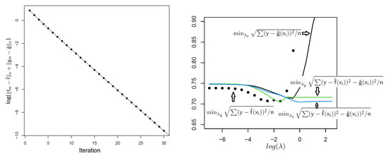
Figure 1. Left panel: Convergence of $f_m,g_m$ using Algorithm 1 for the diabetes dataset. Right panel: For each curve, the label shows which portion (f or g has been subjected to minimization, and the x-axis corresponds to the other $\lambda$ not minimized. The LASSO portion of the elastic net example achieves nearly the same minimum RMSE as the full elastic net for these data, which would be favored in terms of interpretability.

3. Separable Function Classes

Suppose $f^{*}$ and $g^{*}$ can be statistically specified. It can be seen that $\mathcal{F}\cap \mathcal{G}\subset \left\{0\right\}$, for otherwise $f^{*}+w\in \mathcal{F}$ and $g^{*}-w\in \mathcal{G}$ would be another decomposition of h for any $w\in \mathcal{F}\cap \mathcal{G}$. For example, we can consider $\mathcal{A}$ be a function class that h lies in, $\mathcal{F}$ be a subset of $\mathcal{A}$, and $\mathcal{G}={\mathcal{F}}^{\perp }$ be $\mathcal{F}$’s orthogonal complement in $\mathcal{A}$. Nevertheless, we consider a more general case in the sense defined here. We define $\mathcal{F}$ and $\mathcal{G}$ as $L_2$-separable if there exists ${\theta }_1\in [0,1)$ such that for any functions $f\in \mathcal{F}$ and $g\in \mathcal{G}$,

$$\begin{array}{c}\hfill {|⟨f,g⟩}_2|\le {\theta }_1{\parallel f\parallel }_{L_2}{\parallel g\parallel }_{L_2},\end{array}$$

(5)

where ${\parallel f\parallel }_{L_2}$ denotes the $L_2$ norm of a function $f\in L_2(\mathsf{\Omega })$, and ${⟨f,g⟩}_2$ denotes the inner product of functions $f,g\in L_2(\mathsf{\Omega })$. Roughly speaking, the minimal angle of $\mathcal{F}$ and $\mathcal{G}$ is strictly bounded away from zero. If two function classes are $L_2$-separable, then $f^{*}$ and $g^{*}$ are unique, as stated in the following lemma.

Lemma 1.

Suppose (5) is true for any functions $f\in \mathcal{F}$ and $g\in \mathcal{G}$, then $f^{*}$ and $g^{*}$ are unique, up to a difference on a measure zero set (The proof can be found in Appendix B).

3.1. A Separable Additive Model with the Same Covariates

Suppose two function classes $\mathcal{F}\subset H^{{\nu }_1}(\mathsf{\Omega })$, and $\mathcal{G}\subset H^{{\nu }_2}(\mathsf{\Omega })$, where $H^{\nu }(\mathsf{\Omega })$ is the Sobolev space with known smoothness $\nu$. We assume that $\mathcal{F}$ and $\mathcal{G}$ are bounded, i.e., there exist constants $R_1$ and $R_2$ such that ${\parallel f\parallel }_{H^{{\nu }_1}(\mathsf{\Omega })}\le R_1$ and ${\parallel g\parallel }_{H^{{\nu }_2}(\mathsf{\Omega })}\le R_2$, for all $f\in \mathcal{F}$ and $g\in \mathcal{G}$, respectively. Typically, the “easy to interpret” part $\mathcal{F}$ has a higher smoothness, thus we assume ${\nu }_1\ge {\nu }_2$. In order to estimate $f^{*}$ and $g^{*}$, we employ the idea from kernel ridge regression.

Let ${\mathsf{\Psi }}_{\nu }$ be the (isotropic) Matérn family [20], defined by

$$\begin{array}{c}\hfill {\mathsf{\Psi }}_{\nu }(s,t)=\frac{(2\sqrt{{\nu }^{\prime }}{\varphi \parallel s-t\parallel )}^{{\nu }^{\prime }}}{\mathsf{\Gamma }({\nu }^{\prime })2^{{\nu }^{\prime }-1}}{K}_{{\nu }^{\prime }}(2\sqrt{{\nu }^{\prime }}\varphi \parallel s-t\parallel ),\end{array}$$

(6)

where $K_{{\nu }^{\prime }}$ is the modified Bessel function of the second kind, ${\nu }^{\prime }=\nu -p/2$, and $\varphi$ is the range parameter. We use ${\mathcal{N}}_{{\mathsf{\Psi }}_{\nu }}(\mathsf{\Omega })$ to denote the reproducing kernel Hilbert space generated by ${\mathsf{\Psi }}_{\nu }$, and ${\parallel ·\parallel }_{{\mathcal{N}}_{{\mathsf{\Psi }}_{\nu }}(\mathsf{\Omega })}$ to denote the norm of ${\mathcal{N}}_{{\mathsf{\Psi }}_{\nu }}(\mathsf{\Omega })$. By Corollary 10.48 in [21], $H^{\nu }(\mathsf{\Omega })$ coincides with ${\mathcal{N}}_{{\mathsf{\Psi }}_{\nu }}(\mathsf{\Omega })$. We use the solution to

$$\begin{array}{c}\hfill \underset{f\in \mathcal{F},g\in \mathcal{G}}{min}{\parallel y-f-g\parallel }_n^2+{\lambda }_1{\parallel f\parallel }_{{\mathcal{N}}_{{\mathsf{\Psi }}_{{\nu }_1}}(\mathsf{\Omega })}^2+{\lambda }_2{\parallel g\parallel }_{{\mathcal{N}}_{{\mathsf{\Psi }}_{{\nu }_2}}(\mathsf{\Omega })}^2\end{array}$$

(7)

to estimate $f^{*}$ and $g^{*}$, and the corresponding estimators are denoted by $\widehat{f}$ and $\widehat{g}$, respectively. Note that if $\mathcal{G}$ only contains zero function, then (7) reduces to kernel ridge regression. We further require that (5) holds such that $f^{*}$ and $g^{*}$ are identifiable.

First, we consider the consistency of $\widehat{f}$ and $\widehat{g}$, which is provided in the following theorem.

Theorem 2.

Suppose $x_i$’s are uniformly distributed on Ω, and the noise ${ϵ}_i$’s are i.i.d. sub-Gaussian, i.e., satisfying $K^2\mathbb{E}exp(|{ϵ}_i{|}^2/K^2)-1\le {\sigma }_0^2$ for some constants K and ${\sigma }_0^2$, and all $i=1,\dots ,n$. If $max({\lambda }_1,{\lambda }_2)=O_P(n^{-2{\nu }_2/(2{\nu }_2+p)})$, we have (The proof can be found in Appendix C)

$$\begin{array}{c}\hfill \parallel \widehat{g}-g^{*}{\parallel }_{L_2}^2+{\parallel \widehat{f}-f^{*}\parallel }_{L_2}^2=O_P(n^{-\frac{2{\nu }_2}{2{\nu }_2+p}}).\end{array}$$

Remark 2.

Note that in Theorem 2, we only require upper bounds on $max({\lambda }_1,{\lambda }_2)$, which is because $\mathcal{F}$ and $\mathcal{G}$ are bounded. In particular, we can set $max({\lambda }_1,{\lambda }_2)=0$. However, if ${\lambda }_1$ and ${\lambda }_2$ are large, it is more likely that ${\tilde{f}}_m\in \mathcal{F}$ and ${\tilde{g}}_m\in \mathcal{G}$, which allows us to solve (7) efficiently.

Remark 3.

Because $f^{*}$ and $g^{*}$ share the same covariates, the convergence speed of $\widehat{f}-f^{*}$ is slower than the optimal rate $O_P(n^{-\frac{2{\nu }_1}{2{\nu }_1+p}})$. We cannot confirm whether the rate in Theorem 2 is optimal for $\widehat{f}$.

In order to solve the optimization problem in (7), we apply Algorithm 1. In each iteration of Algorithm 1, $g_m$ and $f_m$ are solved by

$$\begin{array}{cc}\hfill g_m=& \underset{g\in \mathcal{G}}{\mathrm{argmin}}\parallel y-f_{m-1}{-g\parallel }_n^2+{\lambda }_2{\parallel g\parallel }_{{\mathcal{N}}_{{\mathsf{\Psi }}_{{\nu }_2}}(\mathsf{\Omega })}^2,\hfill \\ \hfill f_m=& \underset{f\in \mathcal{F}}{\mathrm{argmin}}\parallel y-f-g_m{\parallel }_n^2+{\lambda }_1{\parallel f\parallel }_{{\mathcal{N}}_{{\mathsf{\Psi }}_{{\nu }_1}}(\mathsf{\Omega })}^2,\hfill \end{array}$$

which have explicit forms as

$$\begin{array}{cc}\hfill g_m={\tilde{g}}_m=& r_1{(·)}^T{(K_1+n{\lambda }_1)}^{-1}(Y-f_{m-1}(X)),\hfill \end{array}$$

(8)

$$\begin{array}{cc}\hfill f_m={\tilde{f}}_m=& r_2{(·)}^T{(K_2+n{\lambda }_2)}^{-1}(Y-g_m(X)),\hfill \end{array}$$

(9)

if ${\tilde{g}}_m\in \mathcal{G}$ and ${\tilde{f}}_m\in \mathcal{F}$, where

$$\begin{array}{cc}\hfill r_l(x)=& {({\mathsf{\Psi }}_{{\nu }_l}(x,x_1),\dots ,{\mathsf{\Psi }}_{{\nu }_l}(x,x_n))}^T,\hfill \\ \hfill f_{m-1}(X)=& {(f_{m-1}(x_1),\dots ,f_{m-1}(x_n))}^T,\hfill \\ \hfill g_m(X)=& {(g_m(x_1),\dots ,g_m(x_n))}^T,\hfill \end{array}$$

$K_l={({\mathsf{\Psi }}_{{\nu }_l}(x_j,x_k))}_{jk}$ for $l=1,2$, and $Y={(y_1,\dots ,y_n)}^T$. The explicit forms allow us to solve (17) efficiently.

By Theorem 1, the convergence of Algorithm 1 can be guaranteed. However, if the two function classes separate well, we can achieve a faster convergence, as shown in the following theorem.

Theorem 3.

Suppose two function classes $\mathcal{F}\subset H^{{\nu }_1}(\mathsf{\Omega })$ and $\mathcal{G}\subset H^{{\nu }_2}(\mathsf{\Omega })$ are $L_2$-separable satisfying (5), and $x_i$’s are uniformly distributed on Ω. For $n\ge N$, with probability at least $1-C_{1}exp(-n^{\frac{2{\nu }_2-p}{2{\nu }_2+p}})$, we have either

$$\begin{array}{c}\hfill \parallel f_m-\widehat{f}{\parallel }_n+{\parallel g_{m+1}-\widehat{g}\parallel }_n\le C_2{n}^{-\frac{2{\nu }_2}{2{\nu }_2+p}},\end{array}$$

or

$$\begin{array}{c}\hfill \parallel f_m-\widehat{f}{\parallel }_n+\parallel g_m-\widehat{g}{\parallel }_n\le {\left({\theta }_1+C_3{n}^{-\frac{2{\nu }_2-p}{2(2{\nu }_2+p)}}\right)}^{2m-6}(\parallel f_1-\widehat{f}{\parallel }_n+\parallel g_1-\widehat{g}{\parallel }_n),\end{array}$$

where N and $C_i$’s are constants only depending on $\mathcal{F}$, $\mathcal{G}$ and Ω (The proof can be found in Appendix D).

In the proof of Theorem 3, the key step is to show that with high probability, (5) implies that the separability holds with respect to the empirical norm, i.e.,

$$\begin{array}{c}\hfill {|⟨f,g⟩}_n|\le {\theta }_2{\parallel f\parallel }_n{\parallel g\parallel }_n,\end{array}$$

(10)

with some ${\theta }_2$ close to ${\theta }_1$. It can be seen that in Theorem 3, if $\mathcal{F}$ and $\mathcal{G}$ are separable with respect to the $L_2$ norm, Algorithm 1 achieves a linear convergence. The parameter ${\theta }_1$ determines the convergence speed. If ${\theta }_1$ is small, then the convergence of Algorithm 1 is fast, and a few iterations are enough. By Theorems 2 and 3, it can be seen that the approximation error (the difference between the optimal solution and numerical solution) can be much smaller than the statistical error, which is typical. In particular, we can conclude that the solution obtained by Algorithm 1 satisfies

$$\begin{array}{c}\hfill \parallel f_m-f^{*}{\parallel }_{L_2(\mathsf{\Omega })}+{\parallel g_{m+1}-g^{*}\parallel }_{L_2(\mathsf{\Omega })}\le C_4{n}^{-\frac{{\nu }_2}{2{\nu }_2+p}},\end{array}$$

where we apply Lemma 5.16 of [22], which ensures the asymptotic equivalence of $L_2$ norm and the empirical norm of $\parallel f_m-f^{*}{\parallel }_n$.

3.2. Finite Dimensional Function Classes

As a special case of the model in Section 3.1, suppose two function classes $\mathcal{F}$ and $\mathcal{G}$ have finite dimensions. To be specific, suppose

$$\begin{array}{c}\hfill \mathcal{F}=\left\{f=\sum _{k=1}^{d_1}{\alpha }_k{\varphi }_k:{\alpha }_k\in \mathbb{R},{\parallel f\parallel }_{L_2}\le R_f\right\},\mathcal{G}=\left\{g=\sum _{j=1}^{d_2}{\beta }_j{\phi }_j:{\beta }_k\in \mathbb{R},{\parallel g\parallel }_{L_2}\le R_g\right\},\end{array}$$

where ${\varphi }_k,{\phi }_j$’s are known functions defined on a compact set $\mathsf{\Omega }$, and $R_f$ and $R_g$ are known constants. Furthermore, assume $\mathcal{F}$ and $\mathcal{G}$ are $L_2$-separable. Since the dimension of each function class is finite, we can use the least squares method to estimate $f^{*}$ and $g^{*}$, i.e.,

$$\begin{array}{c}\hfill (\widehat{f},\widehat{g})=\underset{f\in \mathcal{F},g\in \mathcal{G}}{\mathrm{argmin}}{\parallel y-f-g\parallel }_n^2.\end{array}$$

(11)

By applying standard arguments in the theory of Vapnik-Chervonenkis subgraph class [22], the consistency of $\widehat{f}$ and $\widehat{g}$ holds. We do not present detailed discussion for the conciseness of this paper.

Although the exact solution to the optimization problem in (11) is available, we can still use Algorithm 1 to solve it. By comparing the exact solution with numeric solution obtained by Algorithm 1, we can study the convergence rate of Algorithm 1 via numerical simulations. The detailed numerical studies of the convergence rate is provided in Section 5.1.

4. Non-Separable Function Classes

In Section 3, we consider the case that $\mathcal{F}$ and $\mathcal{G}$ are $L_2$-separable, which implies $f^{*}$ and $g^{*}$ are statistically identifiable. However, in many practical cases, $\mathcal{F}$ and $\mathcal{G}$ are not $L_2$-separable. Such examples include $\mathcal{F}$ as a linear function class and $\mathcal{G}$ as the function space generated by a neural network. If $\mathcal{F}$ and $\mathcal{G}$ are not $L_2$-separable, then $f^{*}$ and $g^{*}$ are not statistically identifiable. To see this, note that there exist two sequences of functions $\left\{f_j^{\prime }\right\}\subset \mathcal{F}$ and $\left\{g_j^{\prime }\right\}\subset \mathcal{G}$ such that $\parallel f_j^{\prime }-g_j^{\prime }{\parallel }_{L_2}\to 0$. This implies that $(f^{*},g^{*})$ and $(f^{*}-f_j^{\prime },g^{*}+g_j^{\prime })$ are not statistically identifiable, which implies that we cannot consistently estimate $f^{*}$ and $g^{*}$.

Although $\mathcal{F}$ and $\mathcal{G}$ can be not $L_2$-separable, we can still use (2) to specify $f^{*}$ and $g^{*}$. We propose choosing $\mathcal{F}$ with simple structure and to be “easy to interpret”, and choosing $\mathcal{G}$ to be flexible to improve the prediction accuracy. The tradeoff between interpretation and prediction accuracy can be adjusted by applying different penalty functions $L_f$ and $L_g$. If $L_f$ is large, then (2) forces $f^{*}$ to be small and $g^{*}$ to be large, which indicates that the model is more flexible, but is less interpretable. On the other hand, if $L_g$ is large, then the model is more interpretable, but may reduce the power of prediction.

Another way is to make $\mathcal{F}$ and $\mathcal{G}$ separable. Specifically, suppose $\mathcal{F},\mathcal{G}\subset H^{\nu }(\mathsf{\Omega })$, where $\nu >p/2$ and p is the dimension. Then we construct a new function class ${\mathcal{G}}^{\prime }$ such that ${\mathcal{G}}^{\prime }=\mathcal{G}\cap {\mathcal{F}}^{\perp }$, where ${\mathcal{F}}^{\perp }$ is the perpendicular component of $\mathcal{F}$ in $H^{\nu }(\mathsf{\Omega })$. Although in general, it is not easy to find ${\mathcal{F}}^{\perp }$ (${\mathcal{F}}^{\perp }$ may also be empty), in some cases, it is possible to build ${\mathcal{F}}^{\perp }$, for example, $\mathcal{F}$ is of finite dimension. In the next subsection, we provide a specific example of building the perpendicular component of $\mathcal{F}$ and study the convergence property of its corresponding double penalty model.

A Generalization of Partially Linear Models

In this subsection, we consider a generalization of partially linear models. The responses in a typical partially linear model can be expressed as

$$\begin{array}{c}\hfill y=x^T\beta +g(t)+ϵ.\end{array}$$

(12)

In the partially linear models (12), $\beta \in {\mathbb{R}}^p$ is a vector of regression coefficients associated with x, g is an unknown function of t with some known smoothness, which is usually a one dimensional scalar, and $ϵ$ is a random noise. The partially linear model (12) can be estimated by the partial spline estimator [23,24], partial residual estimator [25,26], or SCAD-penalized regression [27].

In this work, we consider a more general model. Suppose we observe data $y_i$ on $x_i\in \mathsf{\Omega }={[0,1]}^p$ for $i=1,\dots ,n$, where

$$\begin{array}{c}\hfill y_i=x_i^T{\beta }^{*}+g^{*}(x_i)+{ϵ}_i,\end{array}$$

(13)

and ${ϵ}_i$’s are i.i.d. random errors with mean zero and finite variance. We assume that the function $g^{*}\in H^{\nu }(\mathsf{\Omega })$, where $H^{\nu }(\mathsf{\Omega })$ is the Sobolev space with known smoothness $\nu$. This is a standard assumption in nonparametric regression, see [22,28] for example. It is natural to define the two function classes by

$$\begin{array}{c}\hfill \mathcal{F}=\left\{f(x)=x^T\beta :\beta \in {\mathbb{R}}^p,{\parallel \beta \parallel }_2\le R_1,x\in \mathsf{\Omega }\right\}\end{array}$$

and $\mathcal{G}=\{h\in H^{\nu }(\mathsf{\Omega }):\parallel h{\parallel }_{H^{\nu }(\mathsf{\Omega })}\le R_2\}$, where ${\parallel ·\parallel }_2$ denotes the Euclidean distance, and $R_1,R_2$ are known constants. In practice, we can choose a sufficient large $R_1,R_2$ such that $\mathcal{F}$ and $\mathcal{G}$ are large enough. Note that in (13), the linear part and nonlinear part share the same covariates, which is different with (12). It can be seen that ${\beta }^{*}$ and $g^{*}$ are non-identifiable because $\mathcal{F}\subset \mathcal{G}$. Furthermore, $\mathcal{F}$ is more interpretable compared with $\mathcal{G}$ because it is linear.

In order to uniquely identify ${\beta }^{*}$ and $g^{*}$, we need to restrict function class $\mathcal{G}$ such that $\mathcal{F}$ and $\mathcal{G}$ are separable. This can be done by applying a newly developed approach, employing the projected kernel [29]. Let $e_k$, $k=1,\dots ,p$ be an orthonormal basis of $\mathcal{F}$. Then $\mathcal{F}$ can be defined as a linear span of the basis $\{e_1,\dots ,e_p\}$, and the projection of a function $w\in \mathcal{G}$ on $\mathcal{F}$ is given by

$$\begin{array}{c}\hfill {\mathcal{P}}_{\mathcal{F}}w=\sum _{k=1}^p{⟨w,e_k⟩}_2{e}_k.\end{array}$$

(14)

The perpendicular component is

$$\begin{array}{c}\hfill {\mathcal{P}}_{\mathcal{F}}^{\perp }w=w-{\mathcal{P}}_{\mathcal{F}}w.\end{array}$$

(15)

By (14) and (15), we can split $\mathcal{G}$ into two perpendicular classes as $\mathcal{F}$ and ${\mathcal{F}}^{\perp }$, where ${\mathcal{F}}^{\perp }=\{w_1={\mathcal{P}}_{\mathcal{F}}^{\perp }w,w\in \mathcal{G}\}$. Let $h=x^T{\beta }^{*}+g^{*}(x)$, where $g^{*}\in {\mathcal{F}}^{\perp }$. Since $\mathcal{F}$ and ${\mathcal{F}}^{\perp }$ are perpendicular, they are $L_2$-separable. By Lemma 1, ${\beta }^{*}$ and $g^{*}$ are unique. However, in practice it is usually difficult to find a function $g^{*}\in {\mathcal{F}}^{\perp }$ directly. We propose using projected kernel ridge regression, which depends on the reproducing kernel Hilbert space generated by the projected kernel.

The reproducing kernel Hilbert space generated by the projected kernel can be defined in the following way. Define the linear operators ${\mathcal{P}}_{\mathcal{F}}^{(1)}$ and ${\mathcal{P}}_{\mathcal{F}}^{(2)}$: $L_2(\mathsf{\Omega }\times \mathsf{\Omega })\to L_2(\mathsf{\Omega }\times \mathsf{\Omega })$ as

$$\begin{array}{cc}\hfill {\mathcal{P}}_{\mathcal{F}}^{(1)}(u)(x,y)=& \sum _{k=1}^p{e}_k(x){\int }_{\mathsf{\Omega }}u(s,y)e_k(s)ds,\hfill \\ \hfill {\mathcal{P}}_{\mathcal{F}}^{(2)}(u)(x,y)=& \sum _{k=1}^p{e}_k(y){\int }_{\mathsf{\Omega }}u(x,t)e_k(t)dt,\hfill \end{array}$$

for $u\in L_2(\mathsf{\Omega }\times \mathsf{\Omega })$. The projected kernel of $\mathsf{\Psi }$ can be defined by

$$\begin{array}{c}\hfill {\mathsf{\Psi }}_{\mathcal{F}}=\mathsf{\Psi }-{\mathcal{P}}_{\mathcal{F}}^{(1)}\mathsf{\Psi }-{\mathcal{P}}_{\mathcal{F}}^{(2)}\mathsf{\Psi }+{\mathcal{P}}_{\mathcal{F}}^{(1)}{\mathcal{P}}_{\mathcal{F}}^{(2)}\mathsf{\Psi }.\end{array}$$

(16)

The function class ${\mathcal{F}}^{\perp }$ then is equivalent to the reproducing kernel Hilbert space generated by ${\mathsf{\Psi }}_{\mathcal{F}}$, denoted by ${\mathcal{N}}_{{\mathsf{\Psi }}_{\mathcal{F}}}(\mathsf{\Omega })$, and the norm is denoted by ${\parallel ·\parallel }_{{\mathcal{N}}_{{\mathsf{\Psi }}_{\mathcal{F}}}(\mathsf{\Omega })}$. For detailed discussion and properties of ${\mathsf{\Psi }}_{\mathcal{F}}$ and ${\mathcal{N}}_{{\mathsf{\Psi }}_{\mathcal{F}}}(\mathsf{\Omega })$, we refer to [29].

By using the projected kernel of $\mathsf{\Psi }$, the double penalty model is

$$\begin{array}{c}\hfill (\widehat{\beta },\widehat{g})=\underset{\beta \in {\mathbb{R}}^p,g\in {\mathcal{N}}_{{\mathsf{\Psi }}_{\mathcal{F}}}(\mathsf{\Omega })}{\mathrm{argmin}}\parallel y-x^T{\beta -g\parallel }_n^2+\lambda {\parallel g\parallel }_{{\mathcal{N}}_{{\mathsf{\Psi }}_{\mathcal{F}}}(\mathsf{\Omega })}^2,\end{array}$$

(17)

where $(\widehat{\beta },\widehat{g})$ are estimators of $({\beta }^{*},g^{*})$. In practice, we can use generalized cross validation (GCV) to choose the tuning parameter $\lambda$ [29,30]. If the tuning parameter $\lambda$ is chosen properly, we can show that $(\widehat{\beta },\widehat{g})$ are consistent, as stated in the following theorem. In the rest of this paper, we use the following notation. For two positive sequences $a_n$ and $b_n$, we write $a_n\asymp b_n$ if, for some constants $C,C^{\prime }>0$, $C\le a_n/b_n\le C^{\prime }$.

Theorem 4.

Suppose $x_i$’s are uniformly distributed on Ω, and the noise ${ϵ}_i$’s are i.i.d. sub-Gaussian, i.e., satisfying $K^2\mathbb{E}exp(|{ϵ}_i{|}^2/K^2)-1\le {\sigma }_0^2$ for some constants K and ${\sigma }_0^2$, and all $i=1,\dots ,n$. If $\lambda \asymp n^{-2\nu /(2\nu +p)}$, we have

$$\begin{array}{c}\hfill \parallel \widehat{g}-g^{*}{\parallel }_{L_2}^2=O_P(n^{-\frac{2\nu }{2\nu +p}}),{\parallel \widehat{\beta }-{\beta }^{*}\parallel }_2^2=O_P(n^{-\frac{2\nu }{2\nu +p}}).\end{array}$$

Theorem 4 is a direct result of Theorem 3, thus the proof is omitted. Theorem 4 shows that the double penalty model (17) can provide consistent estimators of ${\beta }^{*}$ and $g^{*}$, and the convergence rate of $\parallel \widehat{g}-g^{*}{\parallel }_{L_2}$ is known to be optimal [31]. The convergence rate of $\parallel \widehat{\beta }-{\beta }^{*}{\parallel }_2$ in Theorem 4 is slower than the convergence rate $n^{-1/2}$ in the linear model. We conjecture that this is because the convergence rate is influenced by the estimation of $g^{*}$, which may introduce extra error because functions in ${\mathcal{N}}_{{\mathsf{\Psi }}_{\mathcal{F}}}(\mathsf{\Omega })$ and $\mathcal{F}$ have the same input space.

In order to solve the optimization problem in (17), we apply Algorithm 1. By Theorem 1, the convergence of Algorithm 1 can be guaranteed. In each iteration of Algorithm 1, $g_m$ and $f_m$ are solved by

$$\begin{array}{cc}\hfill g_m=& \underset{g\in {\mathcal{N}}_{{\mathsf{\Psi }}_{\mathcal{F}}}(\mathsf{\Omega })}{\mathrm{argmin}}\parallel y-x^T{\beta }_{m-1}{-g\parallel }_n^2+\lambda {\parallel g\parallel }_{{\mathcal{N}}_{{\mathsf{\Psi }}_{\mathcal{F}}}(\mathsf{\Omega })}^2,\hfill \\ \hfill {\beta }_m=& \underset{\beta \in {\mathbb{R}}^p}{\mathrm{argmin}}{\parallel y-x^T\beta -g_m\parallel }_n^2,\hfill \end{array}$$

which have explicit forms as

$$\begin{array}{cc}\hfill g_m(x)=& r{(x)}^T{(K+n\lambda )}^{-1}(Y-X^T{\beta }_{m-1}),\hfill \\ \hfill {\beta }_m=& {(X^{T}X)}^{-1}{X}^T(Y-g_m(X)),\hfill \end{array}$$

where

$$\begin{array}{cc}\hfill r(x)=& {({\mathsf{\Psi }}_{\mathcal{F}}(x,x_1),\dots ,{\mathsf{\Psi }}_{\mathcal{F}}(x,x_n))}^T,\hfill \\ \hfill g_m(X)=& {(g_m(x_1),\dots ,g_m(x_n))}^T,\hfill \end{array}$$

and $K={({\mathsf{\Psi }}_{\mathcal{F}}(x_j,x_k))}_{jk}$. The explicit forms allow us to solve (17) efficiently. Furthermore, because $\mathcal{F}$ and ${\mathcal{N}}_{{\mathsf{\Psi }}_{\mathcal{F}}}(\mathsf{\Omega })$ are orthogonal, Theorem 3 implies that a few iterations of Algorithm 1 are sufficient to obtain a good numeric solution.

5. Numerical Examples

5.1. Convergence Rate of Algorithm 1

In this subsection, we report numerical studies on the convergence rate of Algorithm 1, and verify that the convergence rate in Theorem 3 is sharp. We consider two finite function classes such that the analytic solution of (11) is available, as stated in Section 3.2. By comparing the numeric solution and the analytic solution, we can verify the convergence rate is sharp.

We consider two function classes $\mathcal{F}=\left\{f\right|f(x)={\alpha }_{1}x,{\alpha }_1\in [0,10]\}$ and $\mathcal{G}=\left\{g\right|g(x)={\alpha }_{2}sin(\theta x),{\alpha }_2\in [0,10]\}$, where $x\in [0,1]$, $\theta$ is a known parameter which controls the degree of separation of two function classes, i.e., the parameter ${\theta }_1$ in Lemma 1. It is easy to verify that for $f\in \mathcal{F}$ and $g\in \mathcal{G}$,

$$\begin{array}{c}\hfill \left|{\int }_0^{1}f(x)g(x)dx\right|\le {\psi (\theta )\parallel f\parallel }_{L_2([0,1])}{\parallel g\parallel }_{L_2([0,1])},\end{array}$$

where

$$\psi (\theta )=\frac{2\sqrt{3\theta }|sin(\theta )-\theta cos(\theta )|}{{\theta }^2\sqrt{2\theta -sin(2\theta )}}.$$

Suppose the underlying function $h(x)={\beta }_1^{*}x+{\beta }_2^{*}sin(\theta x)$ with $({\beta }_1^{*},{\beta }_2^{*})=(1,3)$. Let $({\widehat{\beta }}_1,{\widehat{\beta }}_2)$ be the solution to (11), and $({\beta }_{1,m},{\beta }_{2,m})$ be the values obtained at mth iteration of Algorithm 1. By Theorem 3,

$$\begin{array}{c}\hfill \parallel ({\beta }_{1,m}-{\widehat{\beta }}_1){x\parallel }_n+{\parallel ({\beta }_{2,m}-{\widehat{\beta }}_2)sin(\theta x)\parallel }_n\le C{\left({\theta }_1+C_5{n}^{-\frac{2{\nu }_2-p}{2(2{\nu }_2+p)}}\right)}^{2m-6},\end{array}$$

(18)

where $C=\parallel ({\beta }_{1,1}-{\widehat{\beta }}_1){x\parallel }_2+{\parallel ({\beta }_{2,1}-{\widehat{\beta }}_2)sin(\theta x)\parallel }_2$. By taking logarithms on both sides of (18), we have

$$\begin{array}{cc}\hfill & log(\parallel ({\beta }_{1,m}-{\widehat{\beta }}_1)x{\parallel }_n+\parallel ({\beta }_{2,m}-{\widehat{\beta }}_2)sin(\theta x){\parallel }_n)\hfill \\ \hfill \le & log\left(C{\left({\theta }_1+C_5{n}^{-\frac{2{\nu }_2-p}{2(2{\nu }_2+p)}}\right)}^{2m-6}\right)\hfill \\ \hfill \approx & 2log(\psi (\theta ))m+log(C\psi {(\theta )}^{-6}).\hfill \end{array}$$

(19)

If the convergence rate in Theorem 3 is sharp, then $log(\parallel ({\beta }_{1,m}-{\widehat{\beta }}_1)x{\parallel }_n+\parallel ({\beta }_{2,m}-{\widehat{\beta }}_2)$${sin(\theta x)\parallel }_n)$ is an approximate linear function with respect to m and the slope is close to $2log(\psi (\theta ))$.

In our simulation studies, we choose $\theta =2,3,3.5,4$. We choose the noise $ϵ\sim N(0,0.1)$, where $N(0,0.1)$ is a normal distribution with mean zero and variance $0.1$. The algorithm stops if the left hand side of (18) is less than ${10}^{-6}$. We choose 50 uniformly distributed points as training points. We run 100 simulations and take the average of the regression coefficient and the number of iterations needed for each $\theta$. The results are shown in Table 1.

Table 1. The simulation results when the sample size is fixed. The last column show the absolute difference between the third column and the fourth column, given by $|2log(\psi (\theta ))-$ Regression coefficient|.

$\mathit{\theta }$	$\mathit{\psi }(\mathit{\theta })$	$\mathbf{2}log(\mathit{\psi }(\mathit{\theta }))$	Regression Coefficient	Iteration Numbers	Absolute Difference
2	0.978	−0.045	−0.050	491.55	0.006
3	0.828	−0.378	−0.419	59.02	0.040
3.5	0.615	−0.973	−1.121	22.34	0.148
4	0.304	−2.383	−2.624	10	0.241

Theorem 3 shows that the approximation in (19) is more accurate when the sample size is larger. We conduct numerical studies using sample sizes $20,50,100,150,200$. We choose $\theta =3$. The results are presented in Table 2.

Table 2. The simulation results under different sample sizes. The last column shows the absolute difference between $2log(\psi (3))$ and regression coefficients, given by $|2log(\psi (\theta ))-$ Regression coefficient|.

Sample Size	Regression Coefficient	Iteration Numbers	Absolute Difference
20	−0.110	225.05	0.269
50	−0.410	60.26	0.0315
100	−0.404	61	0.0260
150	−0.363	68	0.0148
200	−0.381	65	0.00244

From Table 1 and Table 2, we find that the absolute difference increases as $\theta$ increases and sample size decreases. When $\psi (\theta )$ decreases, the iteration number decreases, which implies the convergence of Algorithm 1 becomes faster. These results corroborate our theory. The regression coefficients are close to our theoretical assertion $2log(\psi (\theta ))$, which indicates that the convergence rate in Theorem 3 is sharp.

5.2. Prediction of Double Penalty Model

To study the prediction performance of double penalty model, we consider two examples, with $L_2$-separable function classes and non-$L_2$-separable function classes, respectively. In these examples, we would like to stress that we only show the double penalty model can provide relatively accurate estimator with a large part attributing to the “interpretable” part. Since accuracy is not the only goal of our estimator, models that may have extremely high prediction accuracy but may hard to interpret is not preferred in our case. Furthermore, the definition of “interpretable” can be subjective and depends on the user. Therefore, we choose our subjective “interpretable” model in these examples and only show the prediction performance of our model.

Example 1.

Consider function [32]

$$\begin{array}{c}\hfill h(x)=\frac{sin(10\pi x)}{2x}+{(x-1)}^4,x\in [0.5,2.5].\end{array}$$

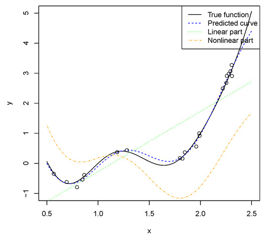
Let $\mathcal{F}=\{f(x)={\beta }_{1}x+{\beta }_2,{\beta }_1^2+{\beta }_2^2\le 100\}$, and $\mathcal{G}$ be the reproducing kernel Hilbert space generated by the projected kernel. The projected kernel is calculated as in (16), where Ψ is as in (6) with $\nu =3.5$ and $\varphi =1$. We use 20 uniformly distributed points from $[0.5,2.5]$ as training points, and let $ϵ\sim N(0,0.1)$. For each simulation, we calculate the mean squared prediction error, which is approximated by calculating the mean squared prediction error on 201 evenly spaced points. We run 100 simulations, and the average mean squared prediction error is 0.016. In this example, the iteration number needed in Algorithm 1 is less than three because the two function classes are orthogonal, which corroborates the results in Theorem 3.

Figure 2 shows that the linear part can capture the trend. However, it can be seen from the figure that the difference between the true function and the linear part is still large. Therefore, a nonlinear part is needed to make good predictions. It also indicates that the function in this example is not easy to interpret.

Figure 2. One simulation result of Example 1 in Section 5.2. Each dot represents an observation on randomly sampled point.

Example 2.

Consider a modified function of [33]

$$\begin{array}{c}\hfill h(x)=\frac{2}{\sqrt{{\sum }_{i=1}^5{(x_i-0.5)}^2}+1}+\frac{0.5}{\sqrt{{\sum }_{i=1}^5{(x_i-0.7)}^2}+1},\end{array}$$

for $x_i\in [0,1]$. We use $\mathcal{F}=\{f(x)={\beta }_1^{T}x+{\beta }_2,\parallel {\beta }_1{\parallel }_2^2+{\beta }_2^2\le \mathrm{10,000},x\in {[0,1]}^5\}$, and $\mathcal{G}$ as the reproducing kernel Hilbert space generated by Ψ, where Ψ is as in (6) with $\nu =3.5$ and $\varphi =1$. Note that $\mathcal{F}$ and $\mathcal{G}$ are not $L_2$-separable because $\mathcal{F}\subset \mathcal{G}$.

The double penalty model is

$$\begin{array}{c}\hfill \underset{\beta \in \mathcal{F},g\in {\mathcal{N}}_{\mathsf{\Psi }}({[0,1]}^5)}{min}\parallel y-x^T{\beta -g\parallel }_n^2+\lambda {\parallel g\parallel }_{{\mathcal{N}}_{\mathsf{\Psi }}({[0,1]}^5)}^2,\end{array}$$

(20)

and the solution is denoted by $(\widehat{\beta },\widehat{g})$. We choose $n\lambda =1,0.1,0.01$, where $n=50$ is the sample size. The noise $ϵ\sim N(0,{\sigma }^2)$, where ${\sigma }^2$ is chosen to be $0.1$ and $0.01$. The iteration numbers are fixed in each simulation, with values $1,2,3,4,5$. We choose maximin Latin hypercube design [34] with sample size 50 as the training set. We run 100 simulations for each case and calculated the mean squared prediction error on the testing set, which is the first 1000 points of the Halton sequence [35].

Table 3 and Table 4 show the simulation results when the variance of noise is 0.1 and 0.01, respectively. We run simulations with iteration numbers $1,2,3,4,5$ for each $n\lambda$, and we find the results are not of much difference. For the briefness, we only present the full simulation results of $n\lambda =1$ to show the similarity, and present the results with 5 iterations for other values of $n\lambda$. In Table 3 and Table 4, we calculate the mean squared prediction error on the training set and the testing set. We also calculate the $L_2$ norm of $\widehat{f}$ and $\widehat{g}$ as in (20), which is approximated by the empirical norm using the first 1000 points of the Halton sequence.

Table 3. Simulation results when $ϵ\sim N(0,0.1)$. The third column shows the mean squared prediction error on the training points. The fourth column shows the mean squared prediction error on the testing points. The fifth column and the last column show the approximated $L_2$ norm of $\widehat{f}$ and $\widehat{g}$ as in (20), respectively.

$\mathit{n}\mathit{\lambda }$	Iteration Number	Training Error	Prediction Error	Linear ${\mathit{L}}_{\mathbf{2}}$	Nonlinear ${\mathit{L}}_{\mathbf{2}}$
1	1	0.02951	0.01714	1.5336	0.0034
	2	0.02950	0.01712	1.5312	0.0054
	3	0.02949	0.01711	1.5288	0.0076
	4	0.02947	0.01710	1.5265	0.0097
	5	0.02946	0.01709	1.5242	0.0119
0.1	5	0.02404	0.01400	1.5264	0.02224
0.001	5	0.0043	0.0059	1.5285	0.1331
$1\times {10}^{-9}$	5	$3.860\times {10}^{-12}$	0.03388	1.5324	0.2174

Table 4. Simulation results when $ϵ\sim N(0,0.01)$. The third column shows the mean squared prediction error on the training points. The fourth column shows the mean squared prediction error on the testing points. The fifth column and the last column show the approximated $L_2$ norm of $\widehat{f}$ and $\widehat{g}$ as in (20), respectively.

$\mathit{n}\mathit{\lambda }$	Iteration Number	Training Error	Prediction Error	Linear ${\mathit{L}}_{\mathbf{2}}$	Nonlinear ${\mathit{L}}_{\mathbf{2}}$
1	1	0.01812	0.01759	1.5316	0.002998
	2	0.01811	0.01757	1.5294	0.004763
	3	0.01810	0.01755	1.5274	0.006664
	4	0.01809	0.01754	1.5253	0.008581
	5	0.01808	0.01753	1.5234	0.010481
0.1	5	0.01336	0.01387	1.5203	0.017585
0.001	5	0.00071	0.00088	1.5287	0.120022

From Table 3 and Table 4, we can obtain the following results: (i) The prediction error in all cases are small, which suggests that the double penalty model can make accurate predictions. (ii) If we increase $n\lambda$, the training error decreases. The prediction error decreases when $n\lambda$ is relatively large, and becomes large when $n\lambda$ is too small. (iii) One iteration in Algorithm 1 is sufficient to obtain a good solution of (20). (iv) The training error of the case with smaller ${\sigma }^2$ is smaller. If $n\lambda$ is chosen properly, the prediction error of the case with smaller ${\sigma }^2$ is small. However, there is not much difference in the prediction error under the cases ${\sigma }^2=0.1$ and $0.01$ when $n\lambda$ is large. (v) For all values of $n\lambda$, the $L_2$ norm of the linear function $\widehat{f}$ does not vary a lot. The $L_2$ norm of $\widehat{g}$, on the other hand, increases as $n\lambda$ decreases. This is because a smaller $n\lambda$ implies a lower penalty on g. (vi) Comparing the values of the $L_2$ norm of $\widehat{f}$ and the $L_2$ norm of $\widehat{g}$, we can see the $L_2$ norm of $\widehat{f}$ is much larger, which is desired because we tend to maximize the interpretable part, which is linear functions in this example.

6. Application to Real Datasets

To illustrate, we apply the approach to two datasets. The first dataset is [36], which includes 50 human fecal microbiome features for $n=414$ unrelated individuals, of genetic sequence tags corresponding to bacterial taxa, and with a response variable of log-transformed body mass index (BMI). To increase the prediction accuracy, we first reduce the number of original features to the final dataset using the HFE cross-validated approach [37], as discussed in [38]. The second dataset is the diabetes dataset from the lars R package, widely used to illustrate penalized regression [39]. The response is a log-transformed measure of disease progression one year after baseline, and predictor features are ten baseline variables, age, sex, BMI, average blood pressure, and six blood serum measurements.

Following Algorithm 1, we let f denote the LASSO algorithm ([40], interpretable part), and use the built-in $l_1$ penalty as $L_f$, with parameter ${\lambda }_f$ as implemented in the R package glmnet. For the “uninterpretable” part, we use the xgboost decision tree approach, with built-in $L_2$ penalty as $L_g$, with parameter ${\lambda }_g$ as implemented in the R package xgboost [41]. For xgboost, we set an $L_1$ penalty as zero throughout, with other parameters (tree depth, etc.), set by cross-validation internally, while preserving convexity of $L_g$. We also set the maximum number of boosting iterations at ten. At each iterative step of LASSO and xgboost, ten simulations of five-fold cross-validation were performed and the predicted values were then averaged.

Finally, in order to explore the tradeoffs between the interpretable and uninterpretable parts, we first establish a range-finding exercise for the penalty tuning parameters on the logarithmic scale, such that ${log}_{10}({\lambda }_g)+{log}_{10}({\lambda }_f)=c$ for constant c. We refer to this tradeoff as the transect between the tuning parameters, with low values of ${\lambda }_f$, for example, emphasizing and placing weight on the interpretable part by enforcing a low penalty for overfitting. To illustrate performance, we use the Pearson correlation coefficient between the response vector y and the average (cross-validated) values of $\widehat{f}$, $\widehat{g}$ and $(\widehat{f}+\widehat{g})$ over the transect. The correlations are of course directly related to the objective function term $\sum {(y-\widehat{f}-\widehat{g})}^2$, but are easier to interpret. Note that $\widehat{f}$ and $\widehat{g}$ are not orthogonal, so the correlations do not partition into the overall correlation of y with $(\widehat{f}+\widehat{g})$. Additionally, as a final comparison, we compute these correlation values over the entire grid of $\{{\lambda }_f,{\lambda }_g\}$ values, to ensure that the transect was largely capturing the best choice of tuning parameters.

For the Goodrich microbiome data, Figure 3 top panel shows the correlations between y and the three cross-validated predictors over the transect. Low values of ${\lambda }_f$ are favored, although it is clear that the decision tree is favored throughout most of the transect, i.e., y has much higher correlations with $\widehat{g}$ than with $\widehat{f}$. Using ${log}_{10}({\lambda }_f)$ in the range of (−2, −1) maximizes the correlation with the interpretable portion, while still achieving near the overall maximum correlation for the combined prediction rule (correlation of nearly 0.5). Our subjective “best balance" region for the interpretable portion is shown on the figure.

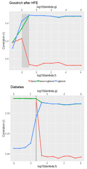
Figure 3. Top panel: cross-validated correlations between y and each of $\widehat{f}$, $\widehat{g}$, and $(\widehat{f}+\widehat{g})$ for the microbiome dataset, where the tuning parameters vary along the transect as described in the text. Bottom panel: the analogous correlations for the diabetes dataset. Grey region and black vertical line represent suggested tuning parameter values to maximize interpretability while preserving high prediction accuracy.

Figure 3 bottom panel shows the analogous results for the diabetes dataset. Here LASSO provides overall good predictions for small tuning parameter ${\lambda }_f$, and ${log}_{10}({\lambda }_f)=-2$ provides good correlations (in the range 0.55–0.6) of y with $\widehat{f}$, $\widehat{g}$ and $(\widehat{f}+\widehat{g})$. As the tuning parameter ${\lambda }_f$ increases, the correlation between y and $\widehat{f}$ falls off dramatically, and our suggested “best balance” point is also shown. In no instance were the correlation values for the full grid of $\{{\lambda }_f,{\lambda }_g\}$ more than 0.015 greater than the greatest value observed along the transects.

7. Discussion

In this work, we propose using a double penalty model as a means of isolating and studying the effects and implications of ensemble learning. We have established conditions for local algorithmic convergence under relatively general convexity conditions. We highlight the fact that in some settings identifiability is not necessary for effective use of the model in prediction. If two function classes are orthogonal, the convergence of the algorithm provided in this work is very fast. This observation inspires potential future work, given any two function classes, to construct two separable function classes that are orthogonal, and to obtain subsequent consistency results, since the two portions are identifiable.

Although our interest here is theoretical, we have also illustrated how the fitting algorithm can be used in practice to make the relative contribution of $\widehat{f}$ large, while not substantially degrading overall predictive performance. The examples here are relatively straightforward, serving to illustrate the theoretical concepts. Further practical implications and implementation issues will be described elsewhere.

References

- Opitz, D.; Maclin, R. Popular ensemble methods: An empirical study. J. Artif. Intell. Res. 1999, 11, 169–198. [Google Scholar] [CrossRef]
- Wolpert, D.H. Stacked generalization. Neural Netw. 1992, 5, 241–259. [Google Scholar] [CrossRef]
- Krogh, A.; Vedelsby, J. Neural network ensembles, cross validation, and active learning. Adv. Neural Inf. Process. Syst. 1994, 7, 231–238. [Google Scholar]
- Wyner, A.J.; Olson, M.; Bleich, J.; Mease, D. Explaining the success of adaboost and random forests as interpolating classifiers. J. Mach. Learn. Res. 2017, 18, 1558–1590. [Google Scholar]
- Breiman, L. Bagging predictors. Mach. Learn. 1996, 24, 123–140. [Google Scholar] [CrossRef]
- Zhang, H.; Nettleton, D.; Zhu, Z. Regression-enhanced random forests. arXiv 2019, arXiv:1904.10416. [Google Scholar]
- Bojer, C.S.; Meldgaard, J.P. Kaggle forecasting competitions: An overlooked learning opportunity. Int. J. Forecast. 2021, 37, 587–603. [Google Scholar] [CrossRef]
- Li, C. A Gentle Introduction to Gradient Boosting. 2016. Available online: http://www.ccs.neu.edu/home/vip/teach/MLcourse/4_boosting/slides/gradient_boosting.pdf (accessed on 1 January 2019).
- Abbott, D. Applied Predictive Analytics: Principles and Techniques for the Professional Data Analyst; John Wiley & Sons: Hoboken, NJ, USA, 2014. [Google Scholar]
- Doshi-Velez, F.; Kim, B. Towards a rigorous science of interpretable machine learning. arXiv 2017, arXiv:1702.08608. [Google Scholar]
- Lundberg, S.M.; Lee, S.I. A unified approach to interpreting model predictions. In Proceedings of the Advances in Neural Information Processing Systems, Long Beach, CA, USA, 4–9 December 2017; pp. 4765–4774. [Google Scholar]
- Ribeiro, M.T.; Singh, S.; Guestrin, C. “Why should i trust you?” Explaining the predictions of any classifier. In Proceedings of the 22nd ACM SIGKDD International Conference on Knowledge Discovery and Data Mining, San Francisco, CA, USA, 13–17 August 2016; pp. 1135–1144. [Google Scholar]
- Bickel, P.J.; Klaassen, C.A.; Bickel, P.J.; Ritov, Y.; Klaassen, J.; Wellner, J.A.; Ritov, Y. Efficient and Adaptive Estimation for Semiparametric Models; Springer: Berlin/Heidelberg, Germany, 1993; Volume 4. [Google Scholar]
- Hastie, T.J.; Tibshirani, R.J. Generalized Additive Models; Routledge: London, UK, 2017. [Google Scholar]
- Ba, S.; Joseph, V.R. Composite Gaussian process models for emulating expensive functions. Ann. Appl. Stat. 2012, 6, 1838–1860. [Google Scholar] [CrossRef]
- Zou, H.; Hastie, T. Regularization and variable selection via the elastic net. J. R. Stat. Soc. Ser. B (Stat. Methodol.) 2005, 67, 301–320. [Google Scholar] [CrossRef]
- Zhou, Q.; Chen, W.; Song, S.; Gardner, J.; Weinberger, K.; Chen, Y. A reduction of the elastic net to support vector machines with an application to GPU computing. In Proceedings of the AAAI Conference on Artificial Intelligence, Austin, TX, USA, 25–30 January 2015; Volume 29. [Google Scholar]
- Zou, H.; Hastie, T.; Tibshirani, R. On the “degrees of freedom” of the lasso. Ann. Stat. 2007, 35, 2173–2192. [Google Scholar] [CrossRef]
- Friedman, J.; Hastie, T.; Tibshirani, R. Regularization paths for generalized linear models via coordinate descent. J. Stat. Softw. 2010, 33, 1. [Google Scholar] [CrossRef] [PubMed]
- Stein, M.L. Interpolation of Spatial Data: Some Theory for Kriging; Springer Science & Business Media: Berlin/Heidelberg, Germany, 1999. [Google Scholar]
- Wendland, H. Scattered Data Approximation; Cambridge University Press: Cambridge, UK, 2004; Volume 17. [Google Scholar]
- van de Geer, S. Empirical Processes in M-Estimation; Cambridge University Press: Cambridge, UK, 2000; Volume 6. [Google Scholar]
- Wahba, G. Partial spline models for the semi-parametric estimation of several variables. In Statistical Analysis of Time Series, Proceedings of the Japan US Joint Seminar; 1984; pp. 319–329. Available online: https://cir.nii.ac.jp/crid/1573387449750539264 (accessed on 27 October 2022).
- Heckman, N.E. Spline smoothing in a partly linear model. J. R. Stat. Soc. Ser. B (Methodol.) 1986, 48, 244–248. [Google Scholar] [CrossRef]
- Speckman, P. Kernel smoothing in partial linear models. R. Stat. Soc. Ser. B (Methodol.) 1988, 50, 413–436. [Google Scholar] [CrossRef]
- Chen, H. Convergence rates for parametric components in a partly linear model. Ann. Stat. 1988, 16, 136–146. [Google Scholar] [CrossRef]
- Xie, H.; Huang, J. SCAD-penalized regression in high-dimensional partially linear models. Ann. Stat. 2009, 37, 673–696. [Google Scholar] [CrossRef]
- Gu, C. Smoothing Spline ANOVA Models; Springer Science & Business Media: Berlin/Heidelberg, Germany, 2013; Volume 297. [Google Scholar]
- Tuo, R. Adjustments to Computer Models via Projected Kernel Calibration. SIAM/ASA J. Uncertain. Quantif. 2019, 7, 553–578. [Google Scholar] [CrossRef]
- Wahba, G. Spline Models for Observational Data; SIAM: Philadelphia, PA, USA, 1990; Volume 59. [Google Scholar]
- Stone, C.J. Optimal global rates of convergence for nonparametric regression. Ann. Stat. 1982, 5, 1040–1053. [Google Scholar] [CrossRef]
- Gramacy, R.B.; Lee, H.K. Cases for the nugget in modeling computer experiments. Stat. Comput. 2012, 22, 713–722. [Google Scholar] [CrossRef]
- Sun, L.; Hong, L.J.; Hu, Z. Balancing exploitation and exploration in discrete optimization via simulation through a Gaussian process-based search. Oper. Res. 2014, 62, 1416–1438. [Google Scholar] [CrossRef]
- Santner, T.J.; Williams, B.J.; Notz, W.I. The Design and Analysis of Computer Experiments; Springer Science & Business Media: Berlin/Heidelberg, Germany, 2003. [Google Scholar]
- Niederreiter, H. Random Number Generation and Quasi-Monte Carlo Methods; SIAM: Philadelphia, PA, USA, 1992; Volume 63. [Google Scholar]
- Goodrich, J.K.; Waters, J.L.; Poole, A.C.; Sutter, J.L.; Koren, O.; Blekhman, R.; Beaumont, M.; Van Treuren, W.; Knight, R.; Bell, J.T. Human genetics shape the gut microbiome. Cell 2014, 159, 789–799. [Google Scholar] [CrossRef] [PubMed]
- Oudah, M.; Henschel, A. Taxonomy-aware feature engineering for microbiome classification. BMC Bioinform. 2018, 19, 227. [Google Scholar] [CrossRef] [PubMed]
- Zhou, Y.H.; Gallins, P. A Review and Tutorial of Machine Learning Methods for Microbiome Host Trait Prediction. Front. Genet. 2019, 10, 579. [Google Scholar] [CrossRef]
- Hastie, T.; Tibshirani, R.; Friedman, J.; Franklin, J. The elements of statistical learning: Data mining, inference and prediction. Math. Intell. 2005, 27, 83–85. [Google Scholar]
- Tibshirani, R. Regression shrinkage and selection via the lasso. J. R. Stat. Soc. Ser. B (Methodol.) 1996, 58, 267–288. [Google Scholar] [CrossRef]
- Chen, T.; Guestrin, C. Xgboost: A scalable tree boosting system. In Proceedings of the 22nd ACM Sigkdd International Conference on Knowledge Discovery and Data Mining, San Francisco, CA, USA, 13–17 August 2016; pp. 785–794. [Google Scholar]
- Adams, R.A.; Fournier, J.J. Sobolev Spaces; Academic Press: Cambridge, MA, USA, 2003; Volume 140. [Google Scholar]
- van de Geer, S. On the uniform convergence of empirical norms and inner products, with application to causal inference. Electron. J. Stat. 2014, 8, 543–574. [Google Scholar] [CrossRef]
Publisher’s Note: MDPI stays neutral with regard to jurisdictional claims in published maps and institutional affiliations. |
© 2022 by the authors. Licensee MDPI, Basel, Switzerland. This article is an open access article distributed under the terms and conditions of the Creative Commons Attribution (CC BY) license (https://creativecommons.org/licenses/by/4.0/).