On the Numerical Solution of 1D and 2D KdV Equations Using Variational Homotopy Perturbation and Finite Difference Methods

Abstract

The KdV equation has special significance as it describes various physical phenomena. In this paper, we use two methods, namely, a variational homotopy perturbation method and a classical finite-difference method, to solve 1D and 2D KdV equations with homogeneous and non-homogeneous source terms by considering five numerical experiments with initial and boundary conditions. The variational homotopy perturbation method is a semi-analytic technique for handling linear as well as non-linear problems. We derive classical finite difference methods to solve the five numerical experiments. We compare the performance of the two classes of methods for these numerical experiments by computing absolute and relative errors at some spatial nodes for short, medium and long time propagation. The logarithm of maximum error vs. time from the numerical methods is also obtained for the experiments undertaken. The stability and consistency of the finite difference scheme is obtained. To the best of our knowledge, a comparison between the variational homotopy perturbation method and the classical finite difference method to solve these five numerical experiments has not been undertaken before. The ideal extension of this work would be an application of the employed methods for fractional and stochastic KdV type equations and their variants.

1. Introduction

Different physical phenomena are modelled using partial differential equations (PDEs) in a variety of applied science fields, including fluid dynamics, cosmology, mathematical biology, quantum physics, chemical kinetics and linear optics. It is well known that the study of non-linear wave equations and their travelling wave solutions is of great importance in various areas. Palencia [1] explored travelling waves and instability in the case of a Fisher–KPP problem with a non-linear advection and a high-order diffusion (see [2,3] and the references therein). Solitary wave solutions of some PDE models have numerous applications in various scientific disciplines, including hydrodynamics, fluid mechanics, plasma physics, plasma waves and chemical physics, condensed matter and solid-state physics [4].

Numerous shallow water wave models have been developed to date [5], notably, the Korteweg–de Vries (KdV) equations, which govern the asymptotic dynamics of wave profiles of long waves in shallow water and are completely integrable. The KdV equation, which was formulated by Korteweg–de Vries in 1895, is recognised as a paradigm for the description of weakly non-linear long waves and is one of the most important non-linear evolution equations in the mathematical sciences [4,6,7,8]. It is given by

$$\begin{array}{c}\hfill {\displaystyle \frac{\partial u(t,x)}{\partial t}}+u(t,x){\displaystyle \frac{\partial u(t,x)}{\partial x}}+{\displaystyle \frac{{\partial }^{3}u(t,x)}{\partial x^3}}=0,\end{array}$$

(1)

where $u(x,t):\mathbb{R}\times {\mathbb{R}}_{+}⟶\mathbb{R}.$ Equation (1) admits solitary wave solutions [9] and is used as a model for ion-acoustic waves [10], non-resonant lattice vibrations, plasma magnetic current waves, pressure gauges for liquid-gas mixtures [7], cosmic inflations [11], long wave propagation through a channel [8], tectonic dynamics and earthquake prediction [12].

In general, the exact solution to the majority of non-linear PDEs may not be found; hence, many analytical techniques have been used for determining an approximate analytical solution. In some instances, the employment of numerical methods is an appropriate alternative. Some of the well-known numerical and analytical techniques used for non-linear PDEs include the spectral method [13], the finite element method [14], the collocation method [15,16,17,18], Adomian’s decomposition method (ADM) [19,20], the variational iteration method (VIM) [21,22,23], and the homotopy perturbation method (HPM) [24,25]. ADM has been applied to solve non-linear equations in [19,20] by separating the equation into linear and non-linear components. The method produces series solutions whose terms are computed from a recursive relation involving the Adomian polynomial, which itself is not an easy problem to address. To overcome these challenges, He [22] explored the variational iteration method (VIM) for solving linear and non-linear problems. We note that VIM was originally referred to in Inokuti et al. [26] as a modification of a general Lagrange multiplier method and it has been found that VIM is user-friendly. VIM was implemented to solve numerous non-linear ODEs and PDEs. VIM does not require exceptional treatment of the non-linear terms as in ADM [27], and it solves linear, as well as non-linear, problems directly. HPM was explored in [24,25] to solve different functional equations, by combining the standard homotopy technique of topology and a perturbation method. HPM has been applied to determine accurate asymptotic solutions for some non-linear PDEs that are used in modelling flows in porous media [28].

Due to the significance of the dispersive KdV equations and their applications, many researchers have been interested in studying various analytical and numerical techniques. These techniques include the differential quadrature method [29], the inverse scattering technique [4], the modified variational iteration technique [30], and the B-spline method [31] for fifth-order KdV equations. Wazwaz [32] applied the variational iteration method (VIM) to solve the Burgers, cubic Boussinesq, KdV, and $\mathrm{K}(2,2)$ equations. Nuruddeen et al. [33] studied a class of fifth-order KdV equations by formulating suitable novel hyperbolic and exponential estimates. The authors in [34] constructed classical and multisymplectic finite difference schemes for linearised KdV equations using numerical experiments and undertook dispersion analysis. Appadu et al. [35] solved some dispersive KdV equations via the LADM, the LADM based on Bernstein polynomials (BLADM), the HPM, and the reduced differential transform method. The authors derived an effective method, BALDM, using Bernstein polynomials, which is applicable to specific types of KdV equations; it was shown that the method diminished the large volume of calculations and its iteration steps towards an exact solution were straightforward. See also recent investigations reported in [36,37,38] for solving the dispersive KdV equations.

The numerical and analytical solutions of two- or higher-dimensional initial boundary value problems of real (or variable) coefficients, both linear and non-linear, are of considerable importance in the applied sciences. The dispersive KdV equation attracted our attention due to its various applications.

Motivated by recent research methodologies that have been developed for PDEs, we consider here an analytical method, known as the variational homotopy perturbation method (VHPM), to solve dispersive 1D and 2D KdV-type equations. VHPM is obtained by combining the homotopy perturbation approach and the variational iteration method [39]. VHPM uses Lagrange multipliers to identify the optimal values of parameters in a functional and homotopy perturbation method. This technique, when used, enables quick and accurate determination of the wave solution to the dispersive KdV equations. The proposed VHPM provides the solution in a quick convergent series, which can lead to a closed form solution and is in good agreement with other semi-analytic approaches [40] in which quite similar problems were solved using a decomposition method. The advantage of the VHPM over decomposition-based approaches is that it solves non-linear problems without the use of Adomian polynomials. For example, the Fisher’s equation is solved using VHPM [41]. It has also been successfully used with non-linear oscillators in [42].

In this investigation, our main objective is not only to apply the variational homotopy perturbation method (VHPM) to determine approximate analytical solutions to various 1D and 2D dispersive Korteweg–de Vries-type equations, but also to construct classical or standard finite difference methods for the experiments undertaken. We compare the performance of the two classes of methods. The investigation involved evaluation of the two methodologies, VHPM and FDM, to determine the most efficient method.

An original contribution of this study is the comparative investigation of the numerical solution of two classes of schemes, namely, the standard finite-difference method and a semi-analytic method, the VHPM, for solving linearised, as well as non-linear dispersive 1D and 2D KdV equations, with some initial and boundary conditions. The reason for working with short propagation times for the experiment pursued is because of their applications in earthquake modelling [12] and the simulation of optical laser pulses along fibres [36], whereas applications for medium and longer propagation times occur, for example, with respect to water waves, sound waves, surface and internal gravity waves arising in various oceanographic conditions [12], oscillations in a solid structure, and electromagnetic radiation [43]. We considered five numerical experiments; using Von Neumann’s analysis, we investigated the stability of the numerical schemes for all the experiments. Analytical proofs of the consistency of the numerical schemes are also given and it is shown that the numerical methods are convergent. The two- and three-dimensional surfaces of the obtained numerical, as well as analytical, solutions are plotted and the maximum error norms vs. time using loglog plots are computed for the experiments.

The remainder of this paper is organised as follows: Section 2 briefly describes the two classes of methods, namely, the semi-analytical variational homotopy perturbation method (VHPM) and the standard finite difference method (FDM). In this section, we describe how both the VHPM and the FDM schemes are constructed to solve the various partial differential equations for the numerical experiments considered. The five numerical experiments are described in Section 3. In Section 4, Section 5, Section 6, Section 7 and Section 8, we analyse the performance of the VHPM and FDM methods for 1D-homogeneous, 1D-non-homogeneous, 2D-homogeneous, 2D-non-homogeneous and 1D-non-homogeneous non-linear KdV equations, respectively. We compare the performance of the numerical schemes using the absolute and relative errors for short, medium and long time propagation. Finally, Section 9 highlights the key features of the paper.

2. The Methods

This section introduces the techniques employed in this paper to solve dispersive KdV problems, namely the standard FDM and VHPM.

2.1. Variational Homotopy Perturbation Method (VHPM)

The variational homotopy perturbation method is derived by combining VIM with HPM. Let us consider a general PDE

$$\begin{array}{c}\hfill \mathcal{L}\left[u\right(t,x\left)\right]+\mathcal{M}\left[u\right(t,x\left)\right]+\mathcal{N}\left[u\right(t,x\left)\right]=g(t,x),\end{array}$$

(2)

where $\mathcal{L}=\frac{\partial }{\partial t}$, $\mathcal{M}$ is a linear operator that includes partial derivatives with respect to x, $\mathcal{N}$ is a non-linear operator and g is a non-homogeneous term, which is u-independent. By relying on VIM in [22,39], the correct functional for the problem in Equation (2) can be written as

$$\begin{array}{c}\hfill u_{n+1}(t,x)=u_n(t,x)+{\int }_0^t\lambda \left(\tau \right)\left\{\mathcal{L}{u}_n(\tau ,x))+\mathcal{M}{u}_n(\tau ,x))+\mathcal{N}{\tilde{u}}_n(\tau ,x)-g(\tau ,x)\right\}\mathrm{d}\tau ,\end{array}$$

(3)

where $\lambda$ is a Lagrange multiplier that can be identified optimally via VIM [22]. Here, ${\tilde{u}}_n$ is considered to be a restricted variation which shows that $\delta {\tilde{u}}_n=0$. Making the correct functional (3) stationary yields

$$\begin{array}{ccc}\hfill \delta v_{n+1}(t,x)& =& \delta v_n(t,x)+\delta {\int }_0^t\lambda \left(\tau \right)\left\{\mathcal{L}{v}_n(\tau ,x))+\mathcal{M}{v}_n(\tau ,x))+\mathcal{N}{\tilde{v}}_n(\tau ,x)-g\left(\tau \right)\right\}\mathrm{d}\tau \hfill \\ & =& \delta v_n(t,x)+{\int }_0^t\delta \left\{\lambda \left(\tau \right)\left(\mathcal{L}{v}_n(\tau ,x))+\mathcal{M}{v}_n(\tau ,x)\right)\right\}\mathrm{d}\tau .\hfill \end{array}$$

(4)

Its stationary conditions can be obtained using the technique of integration in Equation (4). Hence, we obtain [22,23]

$$\begin{array}{c}\hfill \lambda \left(\tau \right)=\frac{{(-1)}^m{(\tau -x)}^{m-1}}{(m-1)!}.\end{array}$$

By applying HPM, we obtain the following relation:

$$\sum _{i=0}^{\infty }{\rho }^i{u}_i(t,x)=u_0(t,x)+\rho \left[{\int }_0^t\lambda \left(\tau \right)\left\{\mathcal{L}\left(\sum _{i=0}^{\infty }{\rho }^i{u}_i\right)+\mathcal{M}\left(\sum _{i=0}^{\infty }{\rho }^i{u}_i\right)+\mathcal{N}\left(\sum _{i=0}^{\infty }{\rho }^i{\tilde{u}}_i\right)\right\}\mathrm{d}\tau -{\int }_0^t\lambda \left(\tau \right)g(\tau ,x)\mathrm{d}\tau \right].$$

(5)

The values $u_0,u_1,u_2,\cdots ,$ are obtained by comparing the like powers of $\rho$. Thus, the approximate solution of Equation (2) can be given as

$$u(t,x)=\underset{\rho \to 1}{lim}\sum _{i=0}^{\infty }{\rho }^i{u}_i(t,x)=u_0(t,x)+u_1(t,x)+u_2(t,x)+\cdots ,$$

(6)

which converges for most cases; it is always assumed that Equation (6) has a unique solution.

2.2. The Standard (Classical) Finite Difference Method

In order to derive the finite difference method for solving 1D and 2D dispersive KdV-type equations, we use the following difference approximations to approximate the derivatives:

$$\begin{array}{cc}\hfill & {\displaystyle \frac{\partial u}{\partial t}}{|}_i^n\approx {\displaystyle \frac{U_i^{n+1}-U_i^{n-1}}{2\Delta t}},\hfill \\ & {\displaystyle \frac{\partial u}{\partial x}}{|}_i^n\approx {\displaystyle \frac{U_{i+1}^n-U_{i-1}^n}{2\Delta x}},\hfill \\ & {\displaystyle \frac{{\partial }^{3}u}{\partial x^3}}{|}_i^n\approx {\displaystyle \frac{U_{i+2}^n-2U_{i+1}^n+2U_{i-1}^n-U_{i-2}^n}{2{(\Delta x)}^3}},\hfill \end{array}$$

where a uniform grid $(x_i,t_n)$ is introduced with

$$\begin{array}{c}\hfill x_i=(i-1)·\Delta x,i=1,\cdots ,\mathrm{N},\mathrm{and}{t}_n=(n-1)·\Delta t,n\in \mathbb{N},\end{array}$$

where $\Delta x$ and $\Delta t$ are the spatial and temporal step sizes, respectively. We obtain the stability region using von Neumann stability analysis and we also study the consistency of the numerical schemes.

3. Numerical Experiments

We solve five problems as detailed below.

(i)

We consider the linear homogeneous dispersive KdV equation [44]

$${\displaystyle \frac{\partial u(t,x)}{\partial t}}+2{\displaystyle \frac{\partial u(t,x)}{\partial x}}+{\displaystyle \frac{{\partial }^{3}u(t,x)}{\partial x^3}}=0,$$

(7)

with $(t,x)\in [0,10.0]\times [0,2\pi ]$, subject to initial conditions [44] $u(0,x)=sin\left(x\right)$ and the boundary conditions: $u(t,0)=-sin\left(t\right)$ and $u(t,2\pi )=sin(2\pi -t)$. The exact solution is given by $u(t,x)=-sin(t-x).$ We used spatial step size $\Delta x=\frac{\pi }{10}$ for this experiment.

(ii)

We consider the linear non-homogeneous dispersive equation [44]

$${\displaystyle \frac{\partial u(t,x)}{\partial t}}+{\displaystyle \frac{{\partial }^{3}u(t,x)}{\partial x^3}}=h(t,x),$$

(8)

with $(t,x)\in [0,1.0]\times [0,1.0],$ and the source term $h(t,x)=-sin\left(t\right)sin\left(\pi x\right)-{\pi }^{3}cos\left(t\right)cos\left(\pi x\right)$, subject to initial conditions $u(0,x)=sin\left(\pi x\right)$, and the boundary conditions are given by $u(t,0)=0$ and $u(t,1.0)=0.$ The exact solution is given by $u(t,x)=cos\left(t\right)sin\left(\pi x\right).$ We used spatial step size $\Delta x=0.05$ for this experiment.

(iii)

We solve the 2D homogeneous equation [44]

$$\begin{array}{c}\hfill {\displaystyle \frac{\partial u(t,x,y)}{\partial t}}+{\displaystyle \frac{{\partial }^{3}u(t,x,y)}{\partial x^3}}+{\displaystyle \frac{{\partial }^{3}u(t,x,y)}{\partial y^3}}=0,\end{array}$$

(9)

with $(t,x,y)\in [0,3.0]\times \mathsf{\Omega },\mathsf{\Omega }=[0,1.0]\times [0,1.0],$ subject to the initial condition

$$\begin{array}{c}\hfill u(0,x,y)=cos(x+y)\end{array}$$

(10)

and the boundary conditions are given by

$$\left.\begin{array}{cc}\hfill u(t,x,0)=cos(2t+x),& u(t,x,1)=cos(1+2t+x),\hfill \\ \hfill u(t,0,y)=cos(2t+y),& u(t,1,y)=cos(2t+1+y).\hfill \end{array}\right\}$$

(11)

The exact solution is $u(t,x,y)=cos(2t+x+y)$. We used $\Delta x=\Delta y=0.1$ for this experiment.

(iv)

We solve the following 2D non-homogeneous equation [43]

$$\begin{array}{c}\hfill {\displaystyle \frac{\partial u(t,x,y)}{\partial t}}+{\displaystyle \frac{{\partial }^{3}u(t,x,y)}{\partial x^3}}+{\displaystyle \frac{{\partial }^{3}u(t,x,y)}{\partial y^3}}=exp\left(t\right)cos(x-y),\end{array}$$

(12)

with $(t,x,y)\in [0,8.0]\times \mathsf{\Omega },\mathsf{\Omega }=[0,1.0]\times [0,1.0],$ subject to the initial condition $u(0,x,y)=sin(x-y)$; the boundary conditions are given by

$$\left.\begin{array}{cc}\hfill u(t,x,0)=exp\left(t\right)cos\left(x\right),& u(t,x,1)=exp\left(t\right)cos(1-x),\hfill \\ \hfill u(t,0,y)=exp\left(t\right)cos\left(y\right),& u(t,1,y)=exp\left(t\right)cos(1-y),\hfill \end{array}\right\}$$

(13)

. The exact solution is $u(t,x,y)=exp\left(t\right)cos(x-y)$. We used $\Delta x=\Delta y=0.1$ for this experiment.

(v)

We solve the dispersive non-linear KdV equation

$$\begin{array}{cc}\hfill & {\displaystyle \frac{\partial u(t,x)}{\partial t}}+6u(x,t){\displaystyle \frac{\partial u(t,x)}{\partial x}}+{\displaystyle \frac{{\partial }^{3}u(t,x)}{\partial x^3}}=0,\hfill \end{array}$$

(14)

where $(t,x)\in [0,1.0]\times [0,2\pi ],$ subject to the initial condition

$$\begin{array}{c}\hfill u(x,0)=\frac{1}{2}{sech}^2\left(\frac{1}{2}x\right),\end{array}$$

(15)

and the boundary conditions are given by

$$\begin{array}{cc}\hfill & u(0,t)=\frac{1}{2}{sech}^2\left(-\frac{t}{2}\right),\mathrm{and}u(2\pi ,t)=\frac{1}{2}{sech}^2\left(\pi -\frac{t}{2}\right);\hfill \\ & {\displaystyle \frac{\partial u}{\partial x}}(0,t)=\frac{1}{2}{sech}^2\left(\frac{t}{2}\right)tanh\left(\frac{t}{2}\right).\hfill \end{array}$$

(16)

The exact solution is $u(x,t)=\frac{1}{2}{sech}^2\left[\frac{1}{2}\left(x-t\right)\right].$ We used spatial step size $\Delta x=\frac{\pi }{10}$ for this experiment.

4. Numerical Experiment 1

4.1. Solution of Numerical Experiment 1 Using VHPM

Let us now rewrite Equation (7) as

$$\mathcal{L}u+\mathcal{M}u=0,$$

where the differential operators are given by $\mathcal{L}={\displaystyle \frac{\partial }{\partial t}}$ and $\mathcal{M}=-2{\displaystyle \frac{\partial }{\partial x}}-{\displaystyle \frac{{\partial }^3}{\partial x^3}}$.

We write Equation (7) as

$$\sum _{i=0}^{\infty }{\rho }^i{u}_i(t,x)=u_0(t,x)-\rho \left[{\int }_0^t\left\{\left(2\sum _{n=0}^{\infty }{\rho }^i{u}_{n,x}+\sum _{n=0}^{\infty }{\rho }^i{u}_{n,xxx}\right)\right\}\mathrm{d}\tau \right],$$

(17)

where $u_{i,x}={\displaystyle \frac{\partial u_i(t,x)}{\partial x}}$ and $u_{i,xxx}={\displaystyle \frac{{\partial }^3{u}_i(t,x)}{\partial x^3}}$. By comparing like terms of $\rho$ on both sides of Equation (17), we obtain the following components:

$$\begin{array}{cc}\hfill & {\rho }^{\left(0\right)}:u_0\left(x\right)=u(0,x)=sin\left(x\right),\hfill \\ & {\displaystyle {\rho }^{\left(1\right)}:u_1(t,x)=-{\int }_0^t\left(2u_{0,x}(\tau ,x)+u_{0,xxx}(\tau ,x)\right)\mathrm{d}\tau =-{\int }_0^{t}cos\left(x\right)\mathrm{d}\tau =-tcos\left(x\right),}\hfill \\ & {\displaystyle {\rho }^{\left(2\right)}:u_2(t,x)=-{\int }_0^t\left(2u_{1,x}(\tau ,x)+u_{1,xxx}(\tau ,x)\right)\mathrm{d}\tau =-{\int }_0^t\tau sin\left(x\right)\mathrm{d}\tau =-{\displaystyle \frac{t^2}{2!}}sin\left(x\right).}\hfill \\ & {\displaystyle {\rho }^{\left(3\right)}:u_3(t,x)=-{\int }_0^t\left(2u_{2,x}(\tau ,x)+u_{2,xxx}(\tau ,x)\right)\mathrm{d}\tau =-{\int }_0^t\left(-{\displaystyle \frac{{\tau }^2}{2!}}cos\left(x\right)\right)\mathrm{d}\tau ={\displaystyle \frac{t^3}{3!}}cos\left(x\right).}\hfill \\ & {\displaystyle {\rho }^{\left(4\right)}:u_4(t,x)=-{\int }_0^t\left(2u_{3,x}(\tau ,x)+u_{3,xxx}(\tau ,x)\right)\mathrm{d}\tau =-{\int }_0^t\left(-{\displaystyle \frac{{\tau }^3}{3!}}sin\left(x\right)\right)\mathrm{d}\tau ={\displaystyle \frac{t^4}{4!}}sin\left(x\right).}\hfill \\ & {\displaystyle {\rho }^{\left(5\right)}:u_5(t,x)=-{\int }_0^t\left(2u_{4,x}(\tau ,x)+u_{4,xxx}(\tau ,x)\right)\mathrm{d}\tau =-{\int }_0^t{\displaystyle \frac{{\tau }^4}{4!}}cos\left(x\right)\mathrm{d}\tau =-{\displaystyle \frac{t^5}{5!}}cos\left(x\right),}\hfill \end{array}$$

and so on. The rest of the components can be obtained in this manner. Thus, the semi-analytical solution with the first ten terms is given by

$$\begin{array}{cc}\hfill u(t,x)& \approx u_0(t;x)+u_1(t;x)+u_2(t;x)+u_3(t;x)+u_4(t;x)+\dots +u_{10}(t;x),\hfill \\ & =sin\left(x\right)-tcos\left(x\right)-{\displaystyle \frac{t^2}{2!}}sin\left(x\right)+{\displaystyle \frac{t^3}{3!}}cos\left(x\right)+{\displaystyle \frac{t^4}{4!}}sin\left(x\right)-{\displaystyle \frac{t^5}{5!}}cos\left(x\right)\hfill \\ & -{\displaystyle \frac{t^6}{6!}}sin\left(x\right)+{\displaystyle \frac{t^7}{7!}}cos\left(x\right)+{\displaystyle \frac{t^8}{8!}}sin\left(x\right)-{\displaystyle \frac{t^9}{9!}}cos\left(x\right)-{\displaystyle \frac{t^{10}}{10!}}sin\left(x\right),\hfill \end{array}$$

which converges to the exact solution $u(t,x)=sin(x-t)$ as required.

In order to verify numerically whether the proposed method leads to higher accuracy, we compute the approximate solution using the n-term sum approximation up to a certain order, say n,

$${\displaystyle \underset{n\to \infty }{lim}{\mathsf{\Psi }}_n(x,t)=u(x,t),}$$

where

$${\displaystyle {\mathsf{\Psi }}_n(x,t)=\sum _{k=0}^n{u}_k(x,t),n\ge 0,}$$

where $u_k$ are the approximate solutions obtained by VHPM. We observe that the numerical and exact profiles are close to each other, especially at low and medium propagation times.

Figure 1 shows the exact solution, as well as the VHPM solution vs. $x\in [0,2\pi ]$ at times $t=0.1,2.0,$ and $4.0$, while Figure 2 depicts plots of the absolute errors versus $x\in [0,2\pi ]$ at some different values of time t.

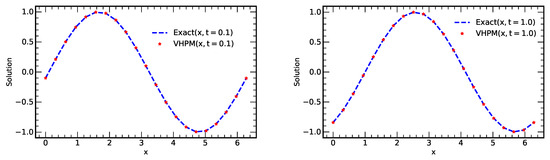
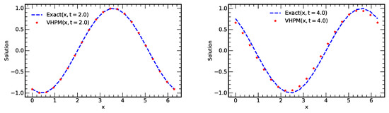
Figure 1. Plots of exact and approximate solutions vs. x using $n=10$ terms from VHPM at times $0.1,1.0,2.0$ and $4.0$. (The spatial step size used is $\frac{\pi }{10})$.

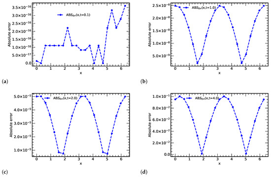
Figure 2. Plots of absolute errors vs. x at some values of time; t = (a) 0.1, (b) 1.0, (c) 2.0, (d) 4.0 using $n=10$ terms from VHPM $\left(\Delta x={\displaystyle \frac{\pi }{10}}\right)$.

4.2. Solution of Numerical Experiment 1 Using Finite Difference Scheme

We consider the homogeneous dispersive KdV equation

$$\begin{array}{c}\hfill {\displaystyle \frac{\partial u(t,x)}{\partial t}}+2{\displaystyle \frac{\partial u(t,x)}{\partial x}}+{\displaystyle \frac{{\partial }^{3}u(t,x)}{\partial x^3}}=0,\end{array}$$

(18)

where $u(x,0)=sin\left(x\right).$ The discretised form of the finite difference scheme for Equation (18) is given by

$$\begin{array}{c}\hfill {\displaystyle \frac{U_i^{n+1}-U_i^{n-1}}{2(\Delta t)}}+2\left({\displaystyle \frac{U_{i+1}^n-U_{i-1}^n}{2(\Delta x)}}\right)+{\displaystyle \frac{U_{i+2}^n-2U_{i+1}^n+2U_{i-1}^n-U_{i-2}^n}{2{(\Delta x)}^3}}=0.\end{array}$$

(19)

Equation (19) can be expressed as

$$\begin{array}{c}\hfill U_i^{n+1}=U_i^{n-1}-2·{\displaystyle \frac{\Delta t}{\Delta x}}·\left(U_{i+1}^n-U_{i-1}^n\right)-{\displaystyle \frac{\Delta t}{{(\Delta x)}^3}}·\left(U_{i+2}^n-2U_{i+1}^n+2U_{i-1}^n-U_{i-2}^n\right),\end{array}$$

(20)

for $i=2,3,\dots ,\mathrm{N}-2$ and $n=2,3,\dots ,\mathrm{Itmax}-1$. (We use N spatial nodes and the number of time nodes is Itmax). To facilitate the numerical computation, we need to use another scheme to obtain the solution at the second time level, using the FTCS scheme:

$$\begin{array}{c}\hfill U_i^2=U_i^1-{\displaystyle \frac{(\Delta t)}{\Delta x}}\left(U_{i+1}^1-U_{i-1}^1\right)-{\displaystyle \frac{(\Delta t)}{2{(\Delta x)}^3}}\left(U_{i+2}^1-2U_{i+1}^1+2U_{i-1}^1-U_{i-2}^1\right),\end{array}$$

for $i=3,4,\dots ,\mathrm{N}-2$ and $n=2,3,\dots ,\mathrm{Itmax}-1$.

The stability region of the scheme can be determined using von Neumann stability analysis on substituting $U_i^n$ with ${\xi }^n{e}^{I\theta ih}$ in Equation (20) to get

$$\begin{array}{c}\hfill \xi ={\xi }^{-1}-2·{\displaystyle \frac{\Delta t}{\Delta x}}·\left(e^{\left(I\omega \right)}-e^{(-I\omega )}\right)-{\displaystyle \frac{\Delta t}{{(\Delta x)}^3}}·\left(e^{\left(2I\omega \right)}-2e^{\left(I\omega \right)}+2e^{(-I\omega )}-e^{(-2I\omega )}\right),\end{array}$$

(21)

where $\omega =\theta h$. Equation (21) can be rewritten as

$$\begin{array}{c}\hfill {\xi }^2=1-2·{\displaystyle \frac{\Delta t}{\Delta x}}·\xi ·(2Isin\left(\omega \right)-{\displaystyle \frac{\Delta t}{{(\Delta x)}^3}}·\left(2Isin\left(2\omega \right)-4Isin\left(\omega \right)\right).\end{array}$$

(22)

The quadratic equation in (22) can be expressed as

$${\xi }^2+I·\mathcal{K}·\xi -1=0,$$

where

$$\mathcal{K}=4·{\displaystyle \frac{\Delta t}{\Delta x}}·sin\left(\omega \right)+2·{\displaystyle \frac{\Delta t}{{(\Delta x)}^3}}·\left(sin\left(2\omega \right)-2sin\left(\omega \right)\right).$$

Solving Equation (22) gives

$$\begin{array}{c}\hfill {\xi }_1={\displaystyle \frac{-I\mathcal{K}+\sqrt{4-{\mathcal{K}}^2}}{2}}\mathrm{and}{\xi }_2={\displaystyle \frac{-I\mathcal{K}-\sqrt{4-{\mathcal{K}}^2}}{2}},\end{array}$$

where ${\xi }_1$ and ${\xi }_2$ are amplification factors of the physical and computational nodes, respectively.

We must have $4-{\mathcal{K}}^2>0$; i.e., $\left|\mathcal{K}\right|<2,$; this then gives $|{\xi }_1|=1$. We solve

$$\begin{array}{c}\hfill |{\displaystyle \frac{4\Delta t}{\Delta x}}sin\left(w\right)+{\displaystyle \frac{2\Delta t}{{(\Delta x)}^3}}\left(sin\left(2w\right)-2sin\left(w\right)\right)|<2.\end{array}$$

(23)

For $\Delta x\to 0$, we see that ${(\Delta x)}^3<<\Delta x$; i.e., ${\displaystyle \frac{1}{{(\Delta x)}^3}}>>{\displaystyle \frac{1}{\Delta x}}$.

By letting $y=sin\left(2\omega \right)-2sin\left(\omega \right)$, we have

$${\displaystyle \frac{dy}{d\omega }}=2cos\left(2\omega \right)-2cos\left(\omega \right).$$

By putting ${\displaystyle \frac{dy}{d\omega }}=0$ and solving for $\omega$, gives $2\left(2{cos}^2\left(\omega \right)-1\right)-2cos\left(\omega \right)=0.$ We, thus, obtain $\omega =0$ or $w=-{\displaystyle \frac{2\pi }{3}}$. Hence, the approximate region of stability, when $\Delta x\to 0$, is given by

$$\begin{array}{c}\hfill |2\sqrt{3}{\displaystyle \frac{\Delta t}{\Delta x}}-{\displaystyle \frac{3\sqrt{3}\Delta t}{{(\Delta x)}^3}}|<2.\end{array}$$

(24)

By choosing $h=\Delta x=\frac{\pi }{10}\approx 0.314$, we obtain

$$\begin{array}{c}\hfill 0<\Delta t\le 0.012774.\end{array}$$

(25)

Consistency

Using Taylor’s series expansion about $(t_n,x_i),$ Equation (20) gives

$$\begin{array}{cc}\hfill & U+(\Delta t)U_t+\frac{{(\Delta t)}^2}{2!}{U}_{tt}+\frac{{(\Delta t)}^3}{3!}{U}_{ttt}+\frac{{(\Delta t)}^4}{4!}{U}_{tttt}+\frac{{(\Delta t)}^5}{5!}{U}_{ttttt}+\mathcal{O}\left({(\Delta t)}^6\right)\hfill \\ & =U-(\Delta t)U_t+\frac{{(\Delta t)}^2}{2!}{U}_{tt}-\frac{{(\Delta t)}^3}{3!}{U}_{ttt}+\frac{{(\Delta t)}^4}{4!}{U}_{tttt}-\frac{{(\Delta t)}^5}{5!}{U}_{ttttt}+\mathcal{O}\left({(\Delta t)}^6\right)\hfill \\ & -\frac{2(\Delta t)}{\Delta x}[U+(\Delta x)U_x+\frac{{(\Delta x)}^2}{2!}{U}_{xx}+\frac{{(\Delta x)}^3}{3!}{U}_{xxx}+\frac{{(\Delta x)}^4}{4!}{U}_{xxxx}+\mathcal{O}\left({(\Delta x)}^5\right)\hfill \\ & -\left(U-(\Delta x)U_x+\frac{{(\Delta x)}^2}{2!}{U}_{xx}-\frac{{(\Delta x)}^3}{3!}{U}_{xxx}+\frac{{(\Delta x)}^4}{4!}{U}_{xxxx}+\mathcal{O}\left({(\Delta x)}^5\right)\right)]\hfill \\ & -\frac{(\Delta t)}{{(\Delta x)}^3}[\left(U+2(\Delta x)U_x+{\displaystyle \frac{{\left(2(\Delta x)\right)}^2}{2}}{U}_{xx}+\frac{{\left(2(\Delta x)\right)}^3}{3!}{U}_{xxx}+\frac{{\left(2(\Delta x)\right)}^4}{4!}{U}_{xxxx}+\frac{(2{\left(\Delta x)\right)}^5}{5!}{U}_{xxxxx}+\mathcal{O}\left({(\Delta x)}^6\right)\right)\hfill \\ & -2\left(U+(\Delta x)U_x+\frac{{(\Delta x)}^2}{2!}{U}_{xx}+\frac{{(\Delta x)}^3}{3!}{U}_{xxx}+\frac{{(\Delta x)}^4}{4!}{U}_{xxxx}+\frac{{(\Delta x)}^5}{5!}{U}_{xxxxx}+\mathcal{O}\left({(\Delta x)}^6\right)\right)\hfill \\ & +2(U-(\Delta x)U_x+\frac{{(\Delta x)}^2}{2!}{U}_{xxx}-\frac{{(\Delta x)}^3}{3!}{U}_{xxx}+\frac{{(\Delta x)}^4}{4!}{U}_{xxxx}-\frac{{(\Delta x)}^5}{5!}{U}_{xxxxx}+\mathcal{O}\left({(\Delta x)}^6\right))\hfill \\ & -\left(U-2(\Delta x)U_x+\frac{{\left(2(\Delta x)\right)}^2}{2!}{U}_{xx}-\frac{{\left(2(\Delta x)\right)}^3}{3!}{U}_{xxx}+\frac{{\left(2(\Delta x)\right)}^4}{4!}{U}_{xxxx}-\frac{{\left(2(\Delta x)\right)}^5}{5!}{U}_{xxxxx}+\mathcal{O}\left({(\Delta x)}^6\right)\right].\hfill \end{array}$$

(26)

After some simplifications, we get

$$\begin{array}{c}\hfill U_t+2U_x+U_{xxx}=-\frac{{(\Delta t)}^2}{3!}{U}_{ttt}-\frac{{(\Delta t)}^4}{5!}{U}_{ttttt}-\frac{2{(\Delta x)}^2}{3!}{U}_{xxx}-\frac{2{(\Delta x)}^4}{5!}{U}_{xxxxx}-\frac{30{(\Delta x)}^2}{5!}{U}_{xxxxx}+\mathcal{O}\left({(\Delta x)}^5\right)+\mathcal{O}\left({(\Delta t)}^5\right).\end{array}$$

(27)

As $\Delta t,\Delta x\to 0$, Equation (27) gives $U_t+2U_x+U_{xxx}=0$ and, therefore, we conclude that the scheme is consistent with Equation (18). The scheme is second-order accurate in time and space.

In Figure 3, we now obtain plots of the numerical and exact profiles vs. x.

Figure 3. Plots of initial, numerical and exact solution vs. $x\in [0,2\pi ]$ at times $t=0.10,2.0,6.0,10.0$, using FDM with $\Delta t={10}^{-3}$ and $\Delta x={\displaystyle \frac{\pi }{10}}$.

The absolute and relative errors vs. x are shown in Figure 4 and Figure 5, respectively, using $\Delta x=\frac{\pi }{10}\approx 0.314$ and $\Delta t={10}^{-3}$.

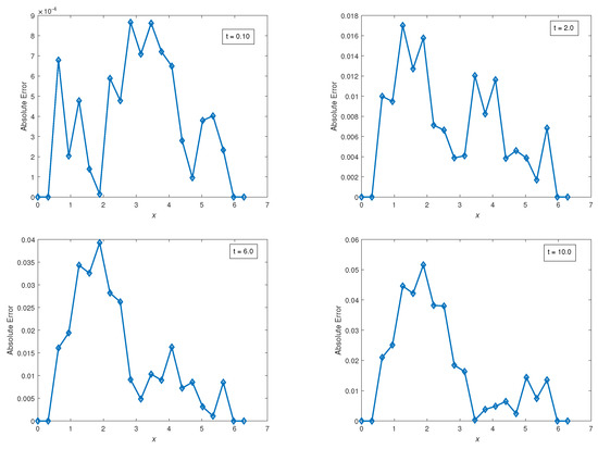
Figure 4. Plots of absolute errors vs. x at times $t=0.10,2.0,6.0,10.0$ using a classical finite difference scheme with $\Delta t={10}^{-3}$ and $\Delta x={\displaystyle \frac{\pi }{10}}$.

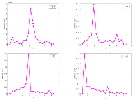
Figure 5. Plots of relative errors vs. x at times $t=0.10,2.0,6.0,10.0$, using a classical finite difference scheme with $\Delta t={10}^{-3}$ and $\Delta x={\displaystyle \frac{\pi }{10}}$.

The following plots give loglog graphs of the maximum error vs. time, $t\in [0,10]$.

We note that Figure 6 compares the effect of the loglog plot of the maximum error vs. time using two different time steps: $\Delta t=0.001$, $0.01$ and with the spatial step $\Delta x=\frac{\pi }{10}$ using the classical FDM for Experiment 1.

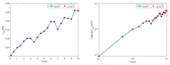
Figure 6. Plots of the maximum error vs. time $t\in [0,10.0]$ and the loglog plot of max. error vs. time using the classical FDM for Experiment 1 with $\Delta t=0.001$, $0.01$ and $\Delta x=\frac{\pi }{10}$.

5. Numerical Experiment 2

5.1. Solution of Experiment 2 Using VHPM

Let us now consider

$${\displaystyle \frac{\partial u(t,x)}{\partial t}}+{\displaystyle \frac{{\partial }^{3}u(t,x)}{\partial x^3}}=h(t,x),$$

(28)

with the source term as given in Equation (8). If we now employ the procedures of VHPM using Equation (5), we can rewrite Equation (8) as

$$\begin{array}{cc}\hfill \sum _{i=0}^{\infty }{\rho }^i{u}_i(t,x)=u_0(t,x)& -\rho \left[{\int }_0^t\lambda \left(\tau \right)\left\{\left(\sum _{n=0}^{\infty }{\rho }^i{u}_{n,xxx}\right)\right\}\mathrm{d}\tau \right]\hfill \\ & -\left[{\int }_0^t\lambda \left(\tau \right)\left\{\left(-{\pi }^{3}cos\left(\pi x\right)cos\left(\tau \right)-sin\left(\pi x\right)sin\left(\tau \right)\right)\right\}\mathrm{d}\tau \right],\hfill \end{array}$$

(29)

where we have $\lambda \left(\tau \right)=-1$, as noted above.

Using Equation (29), the first few VHPM approximation terms are given by

$$\begin{array}{c}{\rho }^{\left(0\right)}:u_0(t,x)=-{\pi }^{3}sin\left(t\right)cos\left(\pi x\right)+cos\left(t\right)sin\left(\pi x\right),\end{array}$$

(30a)

$$\begin{array}{c}{\rho }^{\left(1\right)}:u_1(t,x)={\pi }^{6}sin\left(\pi x\right)+{\pi }^{3}sin\left(t\right)cos\left(\pi x\right)-{\pi }^{6}cos\left(t\right)sin\left(\pi x\right),\end{array}$$

(30b)

$$\begin{array}{c}{\rho }^{\left(2\right)}:u_2(t,x)=-{\pi }^{6}sin\left(\pi x\right)+{\pi }^9\left[t-sin\left(t\right)\right]cos\left(\pi x\right)+{\pi }^{6}cos\left(t\right)sin\left(\pi x\right),\end{array}$$

(30c)

$$\begin{array}{c}{\rho }^{\left(3\right)}:u_3(t,x)={\pi }^{12}sin\left(\pi x\right)-{\pi }^{9}tcos\left(\pi x\right)+{\pi }^{9}sin\left(t\right)cos\left(\pi x\right)-{\pi }^{12}\left[\frac{t^2}{2!}+cos\left(t\right)\right]sin\left(\pi x\right),\end{array}$$

(30d)

$$\begin{array}{c}{\rho }^{\left(4\right)}:u_4(t,x)=-{\pi }^{12}sin\left(\pi x\right)-{\pi }^{15}\left[\frac{t^3}{3!}+sin\left(t\right)\right]cos\left(\pi x\right)+{\pi }^{15}tcos\left(\pi x\right)+{\pi }^{12}sin\left(\pi x\right)\left[\frac{t^2}{2!}+cos\left(t\right)\right],\end{array}$$

(30e)

and so on; in this way the remaining equations of VHPM in the series can be obtained. Thus, the approximate solution to Equation (8), using the first seven terms, is:

$$\begin{array}{c}\hfill {\mathsf{\Psi }}_7(t,x)=-{\pi }^{24}cos\left(t\right)sin\left(\pi x\right)+{\pi }^{24}\left(1-\frac{t^2}{2!}+\frac{t^4}{4!}-\frac{t^6}{6!}+\dots \right)sin\left(\pi x\right)+cos\left(t\right)sin\left(\pi x\right).\end{array}$$

(31)

We observe that Equation (31) converges to the exact solution $u(t,x)=cos\left(t\right)sin\left(\pi x\right)$.

From Figure 7 and Figure 8, we see that VHPM has some challenges for medium and long time propagation; however, it is quite effective for short times for the considered numerical experiment. We note that short time propagation experiments have applications in the analysis of physical phenomena, such as cosmic dynamics [11] and the modelling of earthquakes and tsunamis, as well as oceanographic applications [12].

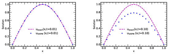
Figure 7. Plots of the exact and approximate solution vs. x at times 0.01, and 0.10 with $\Delta x=0.05$, using $n=7$ terms from VHPM.

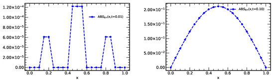
Figure 8. Plots of absolute errors vs. x at times 0.01, and 0.10 with $\Delta x=0.05$ using $n=7$ terms from VHPM.

Remark 1. 

One can observe from Equations (30a)–(30e) the occurrence of noise terms. By ‘noise’ terms, we mean the identical terms, with opposite signs, that may appear in various components $u_j,j\ge 1$ [45,46]. These terms do not show up for homogeneous equations but are used solely for specific types of non-homogeneous equations. A necessary condition for the generation of the noise terms for non-homogeneous problems is that the zeroth component $u_0$ must contain the exact solution u among other terms. For a complete and thorough discussion of noise terms, we refer readers to [46].

5.2. Solution of Numerical Experiment 2 Using Finite Difference Scheme

We propose the following CTCS (CTCS denotes central in time central in space scheme) scheme to discretise Equation (8):

$$\begin{array}{c}\hfill {\displaystyle \frac{U_i^{n+1}-U_i^{n-1}}{2\Delta t}}+{\displaystyle \frac{U_{i+2}^n-2U_{i+1}^n+2U_{i-1}^n-U_{i-2}^n}{2{(\Delta x)}^3}}=-sin\left(t_n\right)sin\left(\pi x_i\right)-{\pi }^{3}cos\left(t_n\right)cos\left(\pi x_i\right).\end{array}$$

(32)

Equation (32) can be rewritten as

$$\begin{array}{c}\hfill U_i^{n+1}=U_i^{n-1}-{\displaystyle \frac{\Delta t}{{(\Delta x)}^3}}(U_{i+2}^n-2U_{i+1}^n+2U_{i-1}^n-U_{i-2}^n)+2\Delta t\left(-sin\left(t_n\right)sin\left(\pi x_i\right)-{\pi }^{3}cos\left(t_n\right)cos\left(\pi x_i\right)\right),\end{array}$$

(33)

for $i=2,3,\dots ,\mathrm{N}-2$ and $n=2,3,\dots ,\mathrm{Itmax}-1$.

To obtain a solution at the second time level, we use the following FTCS scheme (FTCS denotes forward in the time central in space scheme):

$$\begin{array}{c}\hfill {\displaystyle \frac{U_i^{n+1}-U_i^n}{\Delta t}}+{\displaystyle \frac{U_{i+2}^n-2U_{i+1}^n+2U_{i-1}^n-U_{i-2}^n}{2{(\Delta x)}^3}}=-sin\left(\pi x_i\right)sin\left(t_n\right)-{\pi }^{3}cos\left(\pi x_i\right)cos\left(t_n\right),\end{array}$$

(34)

which can be rewritten as

$$\begin{array}{c}\hfill U_i^{n+1}=U_i^n-{\displaystyle \frac{\Delta t}{2{(\Delta x)}^3}}(U_{i+2}^n-2U_{i+1}^n+2U_{i-1}^n-U_{i-2}^n)+\Delta t[-sin\left(\pi x_i\right)sin\left(t_n\right)-{\pi }^{3}cos\left(\pi x_i\right)cos\left(t_n\right)].\end{array}$$

(35)

In order to find the region of stability for Equation (8), we consider Equation (33) with the source term being zero since the source term $g(t,x)$ does not depend on u. We have

$$\begin{array}{c}\hfill U_i^{n+1}=U_i^{n-1}-{\displaystyle \frac{\Delta t}{{(\Delta x)}^3}}·\left(U_{i+2}^n-2U_{i+1}^n+2U_{i-1}^n-U_{i-2}^n\right).\end{array}$$

(36)

By substituting $U_i^n$ by ${\xi }^n{e}^{I\theta ih}$ in Equation (36) and simplifying, we get

$$\begin{array}{c}\hfill \xi ={\xi }^{-1}-{\displaystyle \frac{\Delta t}{{(\Delta x)}^3}}\left(e^{\left(2I\omega \right)}-2e^{\left(I\omega \right)}+2e^{(-I\omega )}-e^{(-2I\omega )}\right),\end{array}$$

(37)

Equation (37) can be expressed as

$$\begin{array}{c}\hfill {\xi }^2+{\displaystyle \frac{\Delta t}{{(\Delta x)}^3}}·\xi ·I·(2sin\left(2\omega \right)-4sin\left(\omega \right))-1=0.\end{array}$$

(38)

Solving Equation (38) yields

$$\begin{array}{c}\hfill \xi ={\displaystyle \frac{-{\displaystyle \frac{\Delta t}{{(\Delta x)}^3}}·I·(2sin(2\omega -4sin\left(\omega \right))\pm \sqrt{4-{\displaystyle \frac{{(\Delta t)}^2}{{(\Delta x)}^6}}(2sin\left(2\omega \right)-4sin{\left(\omega \right))}^2}}{2}}.\end{array}$$

For stability, we need

$${\left[{\displaystyle \frac{\Delta t}{{(\Delta x)}^3}}(2sin\left(2\omega \right)-4sin\left(\omega \right))\right]}^2<4,$$

which simplifies to

$$\left|{\displaystyle \frac{\Delta t}{{(\Delta x)}^3}}(2sin\left(2\omega \right)-4sin\left(\omega \right))\right|<2.$$

We now let $y=2sin\left(2\omega \right)-4sin\left(\omega \right)$. This gives ${\displaystyle \frac{dy}{d\omega }}=8{cos}^2\left(\omega \right)-4cos\left(\omega \right)-4$. By putting ${\displaystyle \frac{dy}{d\omega }}=0$, we obtain $\omega =0,{\displaystyle \frac{-2\pi }{3}},{\displaystyle \frac{2\pi }{3}}$ for $\omega \in [-\pi ,\pi ]$. Thus, the region of stability associated with Equation (8) is given by

$$\begin{array}{c}\hfill {\displaystyle \frac{|\Delta t|}{{|(\Delta x)}^3|}}·\left|2sin\left({\displaystyle \frac{4\pi }{3}}\right)-4sin\left({\displaystyle \frac{2\pi }{3}}\right)\right|<2,\end{array}$$

which simplifies as ${\displaystyle \frac{|\Delta t|}{{|(\Delta x)}^3|}}<{\displaystyle \frac{2}{3\sqrt{3}}}.$

We choose $\Delta x=0.05$ and, therefore, $\Delta t\le 4.811252\times {10}^{-5}.$ (The choice $\Delta x=0.05,\Delta t={10}^{-5}$ is used to run the experiment).

Consistency

We consider Equation (8). The Taylor series expansion about $(t_n,x_i),$ gives

$$\begin{array}{cc}\hfill U+& (\Delta t)U_t+\frac{{(\Delta t)}^2}{2!}{U}_{tt}+\frac{{(\Delta t)}^3}{3!}{U}_{ttt}+\frac{{(\Delta t)}^4}{4!}{U}_{tttt}+\frac{{(\Delta t)}^5}{5!}{U}_{ttttt}+\mathcal{O}\left({(\Delta t)}^6\right)\hfill \\ & =U-(\Delta t)U_t+\frac{{(\Delta t)}^2}{2!}{U}_{tt}-\frac{{(\Delta t)}^3}{3!}{U}_{ttt}+\frac{{(\Delta t)}^4}{4!}{U}_{tttt}-\frac{{(\Delta t)}^5}{5!}{U}_{ttttt}+\mathcal{O}\left({(\Delta t)}^6\right)\hfill \\ & +2(\Delta t)\left[-sin\left(\pi x_i\right)sin\left(t_n\right)-{\pi }^{3}cos\left(\pi x_i\right)cos\left(t_n\right)\right]\hfill \\ & -\frac{(\Delta t)}{{(\Delta x)}^3}·[U+2(\Delta x)U_x+\frac{{\left(2(\Delta x)\right)}^2}{2!}{U}_{xx}+\frac{{\left(2(\Delta x)\right)}^3}{3!}{U}_{xxx}+\frac{{\left(2(\Delta x)\right)}^4}{4!}{U}_{xxxx}+\frac{{\left(2(\Delta x)\right)}^5}{5!}{U}_{xxxxx}+\dots \hfill \\ & -2\left(U+(\Delta x)U_x+\frac{{(\Delta x)}^2}{2!}{U}_{xx}+\frac{{(\Delta x)}^3}{3!}{U}_{xxx}+\frac{{(\Delta x)}^4}{4!}{U}_{xxxx}+\frac{{(\Delta x)}^5}{5!}{U}_{xxxxx}+\dots \right)\hfill \\ & +2(U-(\Delta x)U_x+{\displaystyle \frac{{(\Delta x)}^2}{2!}}{U}_{xx}-\frac{{(\Delta x)}^3}{3!}{U}_{xxx}+\frac{{(\Delta x)}^4}{4!}{U}_{xxxx}-\frac{{(\Delta x)}^5}{5!}{U}_{xxxxx}+\dots )\hfill \\ & -\left(U-2(\Delta x)U_x+\frac{{\left(2(\Delta x)\right)}^2}{2!}{U}_{xx}-\frac{{\left(2(\Delta x)\right)}^3}{3!}{U}_{xxx}+\frac{{\left(2(\Delta x)\right)}^4}{4!}{U}_{xxxx}-\frac{{\left(2(\Delta x)\right)}^5}{5!}{U}_{xxxxx}+\dots \right)].\hfill \end{array}$$

(39)

Simplifying Equation (39) gives

$$\begin{array}{cc}\hfill U_t+U_{xxx}+sin\left(\pi x_i\right)sin\left(t_n\right)+cos\left(\pi x_i\right)cos\left(t_n\right)& =-\frac{{(\Delta t)}^2}{3!}{U}_{ttt}-\frac{{(\Delta t)}^4}{5!}{U}_{ttttt}+\mathcal{O}\left({(\Delta t)}^5\right)\hfill \\ & -\frac{30{(\Delta x)}^2}{5!}{U}_{xxxxx}+\mathcal{O}\left({(\Delta x)}^3\right).\hfill \end{array}$$

Thus, the scheme is consistent and is second-order accurate in time and space.

We obtain plots of the numerical and exact profiles vs. x; the corresponding graphical representations of the absolute and relative errors vs. x are shown in Figure 9 and Figure 10, respectively.

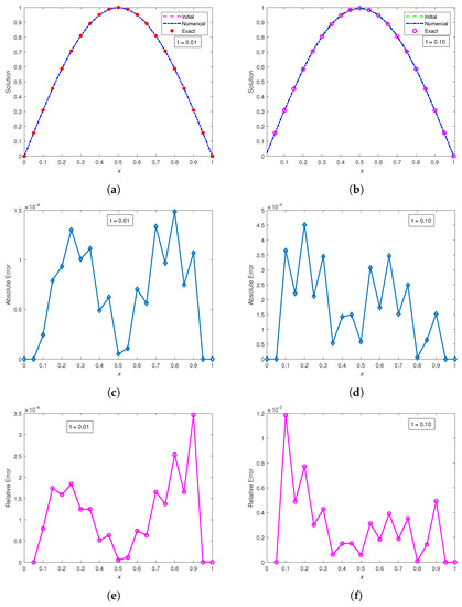
Figure 9. Plots of the exact and numerical solution vs. $x\in [0,1]$ at times $t=0.01,0.10$, using a classical finite difference scheme with $\Delta t={10}^{-5}$, $\Delta x=0.05$ with corresponding absolute and relative errors vs. x (at times $t=0.01,0.10$), respectively. (a) $\Delta t=1.0\times {10}^{-5}$, ($\mathrm{Time}=0.01$); (b) $\Delta t=1.0\times {10}^{-5}$, ($\mathrm{Time}=0.10$); (c) $\Delta t=1.0\times {10}^{-5}$, ($\mathrm{Time}=0.01$); (d) $\Delta t=1.0\times {10}^{-5}$, ($\mathrm{Time}=0.10$); (e) $\Delta t=1.0\times {10}^{-5}$, ($\mathrm{Time}=0.01$); (f) $\Delta t=1.0\times {10}^{-5}$, ($\mathrm{Time}=0.10$).

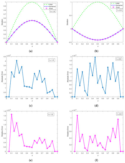
Figure 10. Plots of the exact and numerical solution vs. $x\in [0,1]$ at times $t=1.0,2.0$, using a classical finite difference scheme with $\Delta t={10}^{-5}$, $\Delta x=0.05$, with corresponding absolute and relative errors vs. x (at times $1.0,2.0$), respectively. (a) $\Delta t=1.0\times {10}^{-5}$, ($\mathrm{Time}=1.0$); (b) $\Delta t=1.0\times {10}^{-5}$, ($\mathrm{Time}=2.0$); (c) $\Delta t=1.0\times {10}^{-5}$, ($\mathrm{Time}=1.0$); (d) $\Delta t=1.0\times {10}^{-5}$, ($\mathrm{Time}=2.0$); (e) $\Delta t=1.0\times {10}^{-5}$, ($\mathrm{Time}=1.0$); (f) $\Delta t=1.0\times {10}^{-5}$, ($\mathrm{Time}=2.0$).

Table 1 displays a comparison between the approximate solution and the exact solution together with corresponding absolute and relative errors.

Table 1. Absolute and relative errors at some values of x using a classical finite difference scheme with $\Delta t={10}^{-5}$, $\Delta x=0.05$ at times $t=0.10,1.0,2.0$.

t	x	Exact Solution	Numerical (FDM) Solution	Absolute Error	Relative Error
	0.00	0.000000	0.000000	0.000000	—-
	0.05	0.155653	0.155653	0.0000000	0.000000
	0.10	0.307473	0.307109	3.644020$\times {10}^{-4}$	1.434768$\times {10}^{-3}$
	0.15	0.451722	0.451502	2.209258$\times {10}^{-4}$	3.513621$\times {10}^{-4}$
	0.20	0.584849	0.584398	4.510973$\times {10}^{-4}$	6.214351$\times {10}^{-4}$
	0.25	0.703574	0.703362	2.119868$\times {10}^{-4}$	1.180486$\times {10}^{-4}$
	0.30	0.804975	0.804631	3.446030$\times {10}^{-4}$	4.394541$\times {10}^{-5}$
	0.35	0.886555	0.886501	5.388093$\times {10}^{-5}$	4.614600$\times {10}^{-4}$
	0.40	0.946305	0.946163	1.424468$\times {10}^{-4}$	2.362730$\times {10}^{-4}$
	0.45	0.982754	0.98290	1.486446$\times {10}^{-4}$	5.587316$\times {10}^{-4}$
0.10	0.50	0.995004	0.995063	5.837165$\times {10}^{-5}$	2.152711$\times {10}^{-4}$
	0.55	0.982754	0.98306	3.067277$\times {10}^{-4}$	4.054379$\times {10}^{-4}$
	0.60	0.946305	0.946478	1.731246$\times {10}^{-4}$	5.305065$\times {10}^{-5}$
	0.65	0.886555	0.886901	3.466181$\times {10}^{-4}$	8.155528$\times {10}^{-5}$
	0.70	0.804975	0.805127	1.512676$\times {10}^{-4}$	4.798332$\times {10}^{-4}$
	0.75	0.703574	0.703823	2.488465$\times {10}^{-4}$	3.046279$\times {10}^{-4}$
	0.80	0.584849	0.584854	5.435241$\times {10}^{-6}$	9.697751$\times {10}^{-4}$
	0.85	0.451722	0.451787	6.425356$\times {10}^{-5}$	5.839323$\times {10}^{-4}$
	0.90	0.307473	0.307322	1.516304$\times {10}^{-4}$	1.517804$\times {10}^{-3}$
	0.95	0.155653	0.155653	0.0000000	0.00000000
	1.0	1.218529 $\times {10}^{-16}$	1.218529 $\times {10}^{-16}$	0.000000	0.0000000
	0.00	0.000000	0.000000	0.000000	—
	0.05	8.452190 $\times {10}^{-2}$	8.452190 $\times {10}^{-2}$	0.000000	0.000000
	0.10	1.669626 $\times {10}^{-1}$	1.666859 $\times {10}^{-1}$	2.766808  $\times {10}^{-4}$	1.657142 $\times {10}^{-3}$
	0.15	2.452921 $\times {10}^{-1}$	2.450695 $\times {10}^{-1}$	2.226391  $\times {10}^{-4}$	9.076487 $\times {10}^{-4}$
	0.20	3.175817 $\times {10}^{-1}$	3.171776 $\times {10}^{-1}$	4.041147 $\times {10}^{-4}$	1.272475 $\times {10}^{-3}$
	0.25	3.820514 $\times {10}^{-1}$	3.817850 $\times {10}^{-1}$	2.664477  $\times {10}^{-4}$	6.974131 $\times {10}^{-4}$
	0.30	4.371137 $\times {10}^{-1}$	4.367783 $\times {10}^{-1}$	3.354752 $\times {10}^{-4}$	7.674781 $\times {10}^{-4}$
	0.35	4.814129 $\times {10}^{-1}$	4.812927 $\times {10}^{-1}$	1.202064  $\times {10}^{-4}$	2.496951 $\times {10}^{-4}$
	0.40	5.138580 $\times {10}^{-1}$	5.137448 $\times {10}^{-1}$	1.132063 $\times {10}^{-4}$	2.203066 $\times {10}^{-4}$
	0.45	5.336503 $\times {10}^{-1}$	5.337604 $\times {10}^{-1}$	1.101442  $\times {10}^{-4}$	2.063978 $\times {10}^{-4}$
1.0	0.50	5.403023 $\times {10}^{-1}$	5.403990 $\times {10}^{-2}$	9.664654  $\times {10}^{-5}$	1.788749 $\times {10}^{-4}$
	0.55	5.336503 $\times {10}^{-1}$	5.339099 $\times {10}^{-1}$	2.597111  $\times {10}^{-4}$	4.866691 $\times {10}^{-4}$
	0.60	5.138580 $\times {10}^{-1}$	5.140498 $\times {10}^{-1}$	1.917252  $\times {10}^{-4}$	3.731092 $\times {10}^{-4}$
	0.65	4.814129 $\times {10}^{-1}$	4.817033 $\times {10}^{-1}$	2.903852  $\times {10}^{-4}$	6.031938 $\times {10}^{-4}$
	0.70	4.371137 $\times {10}^{-1}$	4.372791 $\times {10}^{-1}$	1.653917  $\times {10}^{-4}$	3.783723 $\times {10}^{-4}$
	0.75	3.820514 $\times {10}^{-1}$	3.822549 $\times {10}^{-1}$	2.035211 $\times {10}^{-4}$	5.327060 $\times {10}^{-4}$
	0.80	3.175817 $\times {10}^{-1}$	3.176247 $\times {10}^{-1}$	4.299915 $\times {10}^{-5}$	1.353955 $\times {10}^{-4}$
	0.85	2.452921 $\times {10}^{-1}$	2.453477 $\times {10}^{-1}$	5.561969  $\times {10}^{-5}$	2.267488 $\times {10}^{-4}$
	0.90	1.669626  $\times {10}^{-1}$	1.668844 $\times {10}^{-1}$	7.823184  $\times {10}^{-5}$	4.685591 $\times {10}^{-4}$
	0.95	8.452190 $\times {10}^{-2}$	8.452190 $\times {10}^{-2}$	0.000000	0.000000
	1.0	6.616795 $\times {10}^{-17}$	6.616795 $\times {10}^{-17}$	0.000000	0.000000
	0.00	0.000000	0.000000	0.000000	—
	0.05	−6.509971 $\times {10}^{-2}$	−6.509971 $\times {10}^{-2}$	0.000000	0.000000
	0.10	−1.285964 $\times {10}^{-1}$	−1.287342 $\times {10}^{-1}$	1.377844 $\times {10}^{-4}$	1.071448 $\times {10}^{-3}$
	0.15	−1.889267 $\times {10}^{-1}$	−1.889825 $\times {10}^{-1}$	5.578956 $\times {10}^{-5}$	2.952974 $\times {10}^{-4}$
	0.20	−2.446050 $\times {10}^{-1}$	−2.447289 $\times {10}^{-1}$	1.2393035 $\times {10}^{-4}$	5.066551 $\times {10}^{-4}$
	0.25	−2.942603 $\times {10}^{-1}$	−2.942303  $\times {10}^{-1}$	2.990097 $\times {10}^{-5}$	1.01614 $\times {10}^{-4}$
	0.30	−3.366699 $\times {10}^{-1}$	−3.366621 $\times {10}^{-1}$	7.762543  $\times {10}^{-6}$	2.305684 $\times {10}^{-5}$
	0.35	−3.707895 $\times {10}^{-1}$	−3.706230 $\times {10}^{-1}$	1.665078 $\times {10}^{-4}$	4.490629 $\times {10}^{-4}$
	0.40	−3.957792 $\times {10}^{-1}$	−3.956736 $\times {10}^{-1}$	1.055953 $\times {10}^{-4}$	2.668036 $\times {10}^{-4}$
	0.45	−4.110234 $\times {10}^{-1}$	−4.108272 $\times {10}^{-1}$	1.961779 $\times {10}^{-4}$	4.772914 $\times {10}^{-4}$
2.0	0.50	−4.161468 $\times {10}^{-1}$	−4.160785 $\times {10}^{-1}$	6.834419  $\times {10}^{-5}$	1.642310 $\times {10}^{-4}$
	0.55	−4.110234 $\times {10}^{-1}$	−4.109187 $\times {10}^{-1}$	1.046469 $\times {10}^{-4}$	2.546009 $\times {10}^{-4}$
	0.60	−3.957792 $\times {10}^{-1}$	−3.958259 $\times {10}^{-1}$	4.670829  $\times {10}^{-5}$	1.180160 $\times {10}^{-4}$
	0.65	−3.707895 $\times {10}^{-1}$	−3.708076 $\times {10}^{-1}$	1.804617 $\times {10}^{-5}$	4.866957 $\times {10}^{-5}$
	0.70	−3.366699 $\times {10}^{-1}$	−3.368163 $\times {10}^{-1}$	1.464149 $\times {10}^{-4}$	4.348916 $\times {10}^{-4}$
	0.75	−2.942603 $\times {10}^{-1}$	−2.943478 $\times {10}^{-1}$	8.754363 $\times {10}^{-5}$	2.975041 $\times {10}^{-4}$
	0.80	−2.446050 $\times {10}^{-1}$	−2.447732 $\times {10}^{-1}$	1.681892  $\times {10}^{-4}$	6.875951 $\times {10}^{-4}$
	0.85	−1.889267 $\times {10}^{-1}$	−1.890046 $\times {10}^{-1}$	7.784946 $\times {10}^{-5}$	4.120617 $\times {10}^{-4}$
	0.90	−1.285964 $\times {10}^{-1}$	−1.287197 $\times {10}^{-1}$	1.232140 $\times {10}^{-4}$	9.581445 $\times {10}^{-4}$
	0.95	−6.509971 $\times {10}^{-2}$	−6.509971 $\times {10}^{-2}$	0.000000	0.000000
	1.0	−5.096329 $\times {10}^{-17}$	−5.096329 $\times {10}^{-17}$	0.000000	0.000000

Remark 2. 

For the non-homogeneous case (1D space), VHPM faces challenges, even for short time propagation, whereas the classical finite-difference method performs quite well; its relative error ranges from ${10}^{-5}$ to ${10}^{-3}$. The 3D surface plot in Figure 11 for the exact and numerical solution using classical FDM validates the numerical results in Table 1. Figure 12 also shows plots for the maximum error vs. time $t\in [0,2.0]$ and the loglog plot of the maximum error vs. time using the standard FDM for Experiment 2 with $\Delta t={10}^{-5}$ and $\Delta x=0.05$.

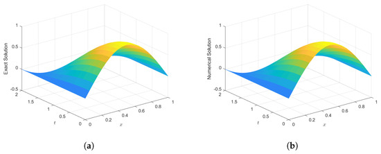
Figure 11. 3D surface plots of the (a) exact solution and (b) numerical solution vs. x at time $2.0$ with $\Delta x=0.05$, using the standard finite difference method.

Figure 12. Plots of the maximum error vs. time $t\in [0,2.0]$, and the loglog plot of max. error vs. time, using the classical FDM with $\Delta t={10}^{-5}$ and $\Delta x=0.05$.

6. Numerical Experiment 3

6.1. Solution of Numerical Experiment 3 Using VHPM

By considering the homogeneous 2D KdV equation in Equation (9), and by applying the VHPM procedure, we have

$$\sum _{i=0}^{\infty }{\rho }^i{u}_i(t,x)=u_0(t,x)+\rho \left[{\int }_0^t(-1)\left\{\sum _{i=0}^{\infty }{\rho }^i{u}_{i,xxx}(\tau ,x)+\sum _{i=0}^{\infty }{\rho }^i{u}_{i,yyy}(\tau ,x)\right\}\mathrm{d}\tau \right].$$

(40)

We then compare the coefficients of $\rho$ on both sides of Equation (40) to obtain

$$\begin{array}{c}{\rho }^{\left(0\right)}:u_0(t,x,y)=cos(x+y),\hfill \end{array}$$

(41a)

$$\begin{array}{cc}& {\displaystyle {\rho }^{\left(1\right)}:u_1(t,x,y)=-{\int }_0^t\left(u_{0,xxx}(\tau ,x,y)+u_{0,yyy}(\tau ,x,y)\right)\mathrm{d}\tau =-{\int }_0^{t}2sin(x+y)\mathrm{d}\tau =-2tcos(x+y),}\hfill \end{array}$$

(41b)

$$\begin{array}{c}{\displaystyle {\rho }^{\left(2\right)}:u_2(t,x,y)=-{\int }_0^t\left(u_{1,xxx}(\tau ,x,y)+u_{1,yyy}(\tau ,x,y)\right)\mathrm{d}\tau =-{\int }_0^{t}4\tau cos(x+y)\mathrm{d}\tau =-\frac{{\left(2t\right)}^2}{2!}cos(x+y),}\hfill \end{array}$$

(41c)

$$\begin{array}{c}{\displaystyle {\rho }^{\left(3\right)}:u_3(t,x,y)=-{\int }_0^t\left(u_{2,xxx}(\tau ,x,y)+u_{2,yyy}(\tau ,x,y)\right)\mathrm{d}\tau =-{\int }_0^{t}4{\tau }^{2}sin(x+y)\mathrm{d}\tau =\frac{{\left(2t\right)}^3}{3!}sin(x+y),}\hfill \end{array}$$

(41d)

and so on. Hence, the sum of the first seven approximate VHPM-terms, as in Equation (41), which are close to the exact solution, is

$$\begin{array}{cc}\hfill {\mathsf{\Psi }}_7(t,x,y)& =cos(x+y)\left[1-\frac{{\left(2t\right)}^2}{2!}+\frac{{\left(2t\right)}^4}{4!}-\frac{{\left(2t\right)}^6}{6!}\right]-sin(x+y)\left[2t-\frac{{\left(2t\right)}^3}{3!}+\frac{{\left(2t\right)}^5}{5!}-\frac{{\left(2t\right)}^7}{7!}\right]\hfill \\ & \approx cos\left(2t\right)cos(x+y)-sin\left(2t\right)sin(x+y)=cos(2t+x+y),\hfill \end{array}$$

which converges to the closed form as required.

For Experiment 3, we present some numerical results in Table 2 and Figure 13.

Table 2. A comparison between the exact solution and VHPM solution at some values of x and y at time $t=0.10,1.0,2.0$.

t	x	y	Exact Solution	VHPM Solution	Absolute Error	Relative Error
	$0.0$	$0.0$	$9.800666\times {10}^{-1}$	$9.800666\times {10}^{-1}$	$6.346390\times {10}^{-11}$	$6.475468\times {10}^{-11}$
	$0.2$	$0.2$	$8.253356\times {10}^{-1}$	$8.253356\times {10}^{-1}$	$5.790479\times {10}^{-11}$	$7.015909\times {10}^{-11}$
		$0.4$	$6.967067\times {10}^{-1}$	$6.967067\times {10}^{-1}$	$5.158263\times {10}^{-11}$	$7.403779\times {10}^{-11}$
		$0.6$	$5.403023\times {10}^{-1}$	$5.403023\times {10}^{-1}$	$4.320399\times {10}^{-11}$	$7.996263\times {10}^{-11}$
		$0.8$	$3.623578\times {10}^{-1}$	$3.623578\times {10}^{-1}$	$3.310296\times {10}^{-11}$	$9.135437\times {10}^{-11}$
$0.10$	$0.4$	$0.2$	$6.967067\times {10}^{-1}$	$6.967067\times {10}^{-1}$	$5.158263\times {10}^{-11}$	$7.403779\times {10}^{-11}$
		$0.4$	$5.403023\times {10}^{-1}$	$5.403023\times {10}^{-1}$	$4.320399\times {10}^{-11}$	$7.996263\times {10}^{-11}$
		$0.6$	$3.623578\times {10}^{-1}$	$3.623578\times {10}^{-1}$	$3.310296\times {10}^{-11}$	$9.135437\times {10}^{-11}$
		$0.8$	$1.699671\times {10}^{-1}$	$1.699671\times {10}^{-1}$	$2.168213\times {10}^{-11}$	$1.275666\times {10}^{-10}$
	$0.8$	$0.2$	$3.623578\times {10}^{-1}$	$3.623578\times {10}^{-1}$	$3.310296\times {10}^{-11}$	$9.135437\times {10}^{-11}$
		$0.4$	$1.699671\times {10}^{-1}$	$1.699671\times {10}^{-1}$	$2.168213\times {10}^{-11}$	$1.275666\times {10}^{-10}$
		$0.6$	$-2.919952\times {10}^{-2}$	$-2.919952\times {10}^{-2}$	$9.39695\times {10}^{-12}$	$3.218185\times {10}^{-10}$
		$0.8$	$-2.272021\times {10}^{-1}$	$-2.272021\times {10}^{-1}$	$3.262889\times {10}^{-12}$	$1.436118\times {10}^{-11}$
	$1.0$	$1.0$	$-5.885011\times {10}^{-1}$	$-5.885011\times {10}^{-1}$	$2.769285\times {10}^{-11}$	$4.705658\times {10}^{-11}$
	$0.0$	$0.0$	$-4.161468\times {10}^{-1}$	$-4.222222\times {10}^{-1}$	$6.075386\times {10}^{-3}$	$1.459914\times {10}^{-2}$
	$0.2$	$0.2$	$-7.373937\times {10}^{-1}$	$-7.424596\times {10}^{-1}$	$5.065830\times {10}^{-3}$	$6.869920\times {10}^{-3}$
		$0.4$	$-8.568888\times {10}^{-1}$	$-8.611346\times {10}^{-1}$	$4.245800\times {10}^{-3}$	$4.954900\times {10}^{-3}$
		$0.6$	$-9.422223\times {10}^{-1}$	$-9.454788\times {10}^{-1}$	$3.256500\times {10}^{-3}$	$3.456190\times {10}^{-3}$
		$0.8$	$-9.899925\times {10}^{-1}$	$-9.921299\times {10}^{-1}$	$2.137370\times {10}^{-3}$	$2.158980\times {10}^{-3}$
$1.0$	$0.4$	$0.2$	$-8.5688875\times {10}^{-1}$	$-8.611346\times {10}^{-1}$	$4.245800\times {10}^{-3}$	$4.954900\times {10}^{-3}$
		$0.4$	$-9.422223\times {10}^{-1}$	$-9.454788\times {10}^{-1}$	$3.256500\times {10}^{-3}$	$3.456190\times {10}^{-3}$
		$0.6$	$-9.899925\times {10}^{-1}$	$-9.921299\times {10}^{-1}$	$2.137370\times {10}^{-3}$	$2.158980\times {10}^{-3}$
		$0.8$	$-9.982948\times {10}^{-1}$	$-9.992278\times {10}^{-1}$	$9.330300\times {10}^{-4}$	$9.346300\times {10}^{-4}$
	$0.8$	$0.2$	$-9.899925\times {10}^{-1}$	$-9.9212987\times {10}^{-1}$	$2.137370\times {10}^{-3}$	$2.158980\times {10}^{-3}$
		$0.4$	$-9.982948\times {10}^{-1}$	$-9.992278\times {10}^{-1}$	$9.330300\times {10}^{-4}$	$9.346300\times {10}^{-4}$
		$0.6$	$-9.667982\times {10}^{-1}$	$-9.664897\times {10}^{-1}$	$3.085000\times {10}^{-4}$	$3.191000\times {10}^{-4}$
		$0.8$	$-8.967584\times {10}^{-1}$	$-8.952207\times {10}^{-1}$	$1.537740\times {10}^{-3}$	$1.714770\times {10}^{-3}$
	$1.0$	$1.0$	$-6.536436\times {10}^{-1}$	$-6.498779\times {10}^{-1}$	$3.765733\times {10}^{-3}$	$5.761140\times {10}^{-3}$
	$0.0$	$0.0$	$-6.536436\times {10}^{-1}$	$-2.022222$	$1.368579\times {10}^0$	$2.093768\times {10}^0$
	$0.2$	$0.2$	$-3.073329\times {10}^{-1}$	$-1.323586\times {10}^0$	$1.016253\times {10}^0$	$3.306684\times {10}^0$
		$0.4$	$-1.121525\times {10}^{-1}$	$-8.874751\times {10}^{-1}$	$7.753226\times {10}^{-1}$	$6.913109\times {10}^0$
		$0.6$	$8.749898\times {10}^{-2}$	$4.159839\times {10}^{-1}$	$5.034829\times {10}^{-1}$	$5.754156\times {10}^0$
		$0.8$	$2.836622\times {10}^{-1}$	$7.209137\times {10}^{-2}$	$2.115708\times {10}^{-1}$	$7.458549\times {10}^{-1}$
	$0.4$	$0.2$	$-1.121525\times {10}^{-1}$	$-8.874751\times {10}^{-1}$	$7.753226\times {10}^{-1}$	$6.91311\times {10}^0$
2.0		$0.4$	$8.749898\times {10}^{-2}$	$-4.159839\times {10}^{-1}$	$5.034829\times {10}^{-1}$	$5.754157\times {10}^0$
		$0.6$	$2.836622\times {10}^{-1}$	$7.209137\times {10}^{-2}$	$2.115708\times {10}^{-1}$	$7.458548\times {10}^{-1}$
		$0.8$	$4.685167\times {10}^{-1}$	$5.572926\times {10}^{-1}$	$8.877587\times {10}^{-2}$	$1.894828\times {10}^{-1}$
	$0.8$	$0.2$	$2.836622\times {10}^{-1}$	$7.209137\times {10}^{-2}$	$2.115708\times {10}^{-1}$	$7.458548\times {10}^{-1}$
		$0.4$	$4.685167\times {10}^{-1}$	$5.572926\times {10}^{-1}$	$8.877587\times {10}^{-2}$	$1.894828\times {10}^{-1}$
		$0.6$	$6.346929\times {10}^{-1}$	$1.020276\times {10}^0$	$3.855834\times {10}^{-1}$	$6.075117\times {10}^{-1}$
		$0.8$	$7.755659\times {10}^{-1}$	$1.442585\times {10}^0$	$6.670188\times {10}^{-1}$	$8.600415\times {10}^{-1}$
	$1.0$	$1.0$	$9.601703\times {10}^{-1}$	$2.100124\times {10}^0$	$1.139954\times {10}^0$	$1.187242\times {10}^0$

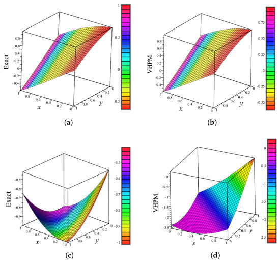
Figure 13. 3D graphical representation of the exact solution and approximate solutions vs. x vs. y using $n=7$ terms from VHPM for Equation (9) at times $t=0.10,1.0$, respectively. (a) $t=0.10$; (b) $t=0.10$; (c) $t=1.0$; (d) $t=1.0$.

The following graphics in Figure 13 show the results of the exact and approximate solutions using VHPM; the behaviour of the numerical results is shown in Table 2.

Remark 3. 

Table 2 compares the exact solution with the VHPM solution with corresponding absolute and relative errors at some values of x and y, and at times $t=0.10$, $t=1.0$ and $t=2.0$, respectively. Figure 13 depicts the 3D graphs of the exact and approximate solution vs. x vs. y using $n=7$ terms from the VHPM. From the numerical results, one can see that the VHPM solution is effective for short time propagation and may struggle to achieve accuracy for long time propagation.

6.2. Solution of Numerical Experiment 3 Using Finite Difference Scheme

In order to construct a classical finite difference method to solve numerical Experiment 3, we use the following central difference approximations:

$$\left.\begin{array}{cc}\hfill \begin{array}{c}\hfill \end{array}& {\displaystyle \frac{\partial u}{\partial t}}{|}_{i,j}^n\approx {\displaystyle \frac{U_{i,j}^{n+1}-U_{i,j}^{n-1}}{2·\Delta t}},\hfill \\ & {\displaystyle \frac{\partial u}{\partial x}}{|}_{i,j}^n\approx {\displaystyle \frac{U_{i+1,j}^n-U_{i-1,j}^n}{2·\Delta x}},\hfill \\ & {\displaystyle \frac{{\partial }^{3}u}{\partial x^3}}{|}_{i,j}^n\approx {\displaystyle \frac{U_{i+2,j}^n-2U_{i+1,j}^n+2U_{i-1,j}^n-U_{i-2,j}^n}{2·{(\Delta x)}^3}},\hfill \\ & {\displaystyle \frac{{\partial }^{3}u}{\partial y^3}}{|}_{i,j}^n\approx {\displaystyle \frac{U_{i,j+2}^n-2U_{i,j+1}^n+2U_{i,j-1}^n-U_{i,j-2}^n}{2·{(\Delta y)}^3}}.\hfill \end{array}\right\}$$

We point out that a rectangular domain is divided into square grids with each x and y interval of length $\Delta x$ and $\Delta y$, respectively, whereas each t-interval is of length $\Delta t$. A uniform grid $\Delta x=\Delta y=h$ is considered with

$$\begin{array}{cc}\hfill x_i& =(i-1)·\Delta x=(i-1)·h,i=1,\dots ,\mathrm{N},\hfill \\ \hfill y_j& =(j-1)·\Delta y=(j-1)·h,j=1,\dots ,\mathrm{N},\hfill \\ \hfill t_n& =(n-1)·\Delta t=(n-1)·k,n\in \mathbb{N}.\hfill \end{array}$$

The scheme is given by

$$\begin{array}{c}\hfill \frac{U_{i,j}^{n+1}-U_{i,j}^{n-1}}{2\Delta t}=-\left(\frac{U_{i+2,j}^n-2U_{i+1,j}^n+2U_{i-1,j}^n-U_{i-2,j}^n}{2·{(\Delta x)}^3}\right)-\left(\frac{U_{i,j+2}^n-2U_{i,j+1}^n+2U_{i,j-1}^n-U_{i,j-2}^n}{2·{(\Delta y)}^3}\right).\end{array}$$

Hence, the numerical scheme takes the form

$$\begin{array}{c}\hfill U_{i,j}^{n+1}=U_{i,j}^{n-1}-r_x\left(U_{i+2,j}^n-2U_{i+1,j}^n+2U_{i-1,j}^n-U_{i-2,j}^n\right)-r_y\left(U_{i,j+2}^n-2U_{i,j+1}^n+2U_{i,j-1}^n-U_{i,j-2}^n\right),\end{array}$$

(42)

where

$$\begin{array}{c}\hfill r_x={\displaystyle \frac{\Delta t}{{(\Delta x)}^3}}\mathrm{and}{r}_y={\displaystyle \frac{\Delta t}{{(\Delta y)}^3}}.\end{array}$$

(43)

By substituting $U_{i,j}^n$ by ${\xi }^n·e^{I{\omega }_{x}i}·e^{I{\omega }_{y}j},$ we obtain

$$\begin{array}{cc}\hfill {\xi }^{n+1}exp\left[I({\omega }_{x}i+{\omega }_{y}j)\right]& ={\xi }^{n-1}exp\left[I({\omega }_{x}i+{\omega }_{y}j)\right]-{\displaystyle \frac{\Delta t}{{(\Delta x)}^3}}({\xi }^{n}exp\left[I({\omega }_x(i+2)+{\omega }_{y}j)\right]-2{\xi }^{n}exp\left[I({\omega }_x(i+1)+{\omega }_{y}j)\right]\hfill \\ & +2{\xi }^{n}exp\left[I({\omega }_x(i-1)+{\omega }_{y}j)\right]-{\xi }^{n}exp\left[I({\omega }_x(i-2)+{\omega }_{y}j)\right])\hfill \\ & -{\displaystyle \frac{\Delta t}{{(\Delta y)}^3}}({\xi }^{n}exp\left[I({\omega }_{x}i+{\omega }_y(j+2))\right]-2{\xi }^{n}exp\left[I({\omega }_{x}i+{\omega }_y(j+1))\right]\hfill \\ & +2{\xi }^{n}exp\left[I({\omega }_{x}i+{\omega }_y(j-1))\right]-{\xi }^{n}exp\left[I({\omega }_{x}i+{\omega }_y(j-2))\right]).\hfill \end{array}$$

(44)

By dividing both sides of Equation (44) with ${\xi }^n{e}^{I({\omega }_{x}i+{\omega }_{y}j)}$, we have

$$\begin{array}{cc}\hfill & {\xi }^2=1-{\displaystyle \frac{\Delta t}{{(\Delta x)}^3}}\left(\xi exp\left[2I{\omega }_x\right]-2\xi exp\left[I{\omega }_x\right]+2\xi exp\left[-I{\omega }_x\right]-\xi exp\left[-2I{\omega }_x\right]\right)\hfill \\ & -{\displaystyle \frac{\Delta t}{{(\Delta y)}^3}}\left(\xi exp\left[2I{\omega }_y\right]-2\xi exp\left[I{\omega }_y\right]+2\xi exp\left[-I{\omega }_y\right]-\xi exp\left[-2I{\omega }_y\right]\right),\hfill \end{array}$$

(45)

Equation (45) can be expressed as

$$\begin{array}{c}\hfill {\xi }^2=1-{\displaystyle \frac{\Delta t}{{(\Delta x)}^3}}·\left(\xi .I.\left(2sin\left(2{\omega }_x\right)-4sin\left({\omega }_x\right)\right)\right)-{\displaystyle \frac{\Delta t}{{(\Delta y)}^3}}·\left(\xi .I.\left(2sin\left(2{\omega }_y\right)-4sin\left({\omega }_y\right)\right)\right),\end{array}$$

which simplifies to

$$\begin{array}{c}\hfill {\xi }^2+2·\mathcal{B}(x,y)·I·\xi -1=0,\end{array}$$

(46)

where

$$\mathcal{B}(x,y)=r_x·\left(sin\left({\omega }_x\right)-2sin\left({\omega }_x\right)\right)+r_y·\left(sin\left(2{\omega }_y\right)-2sin\left({\omega }_y\right)\right),$$

and $r_x$ and $r_y$ are given as in Equation (43). By solving the quadratic equation in Equation (46), we obtain

$$\begin{array}{c}\hfill \xi ={\displaystyle \frac{1}{2}}\left(-2\mathcal{B}(x,y)·I\pm \sqrt{4-4{\mathcal{B}}^2(x,y)}\right)\end{array}$$

A condition for the stability criterion is determined by finding a condition for $\Delta t,\Delta x$, so that, for all $\theta ,\xi$

$$\begin{array}{c}\hfill |\xi ({\omega }_x,{\omega }_y)|\le 1\mathrm{holds};\mathrm{i}.\mathrm{e}.,1-{\mathcal{B}}^2(x,y)\ge 0\Rightarrow \left|\mathcal{B}(x,y)\right|\le 1.\end{array}$$

(47)

Hence, Equation (47) is equivalently expressed as

$$\begin{array}{c}\hfill |r_x·\left(sin\left(2{\omega }_x\right)-2sin\left({\omega }_x\right)\right)+r_y·\left(sin\left(2{\omega }_y\right)-2sin\left({\omega }_y\right)\right)|\le 1.\end{array}$$

We fixed $\Delta x=\Delta y=0.1$. For stability, we need to solve

$$\begin{array}{c}\hfill \left|\mathsf{\Psi }\right({\omega }_x,{\omega }_y,\Delta t\left)\right|\le 1,\end{array}$$

$$\mathrm{with}\mathsf{\Psi }({\omega }_x,{\omega }_y,\Delta t)={\displaystyle \frac{\Delta t}{{\left(0.1\right)}^3}}·\left(sin\left(2{\omega }_x\right)-2sin\left({\omega }_x\right)\right)+{\displaystyle \frac{\Delta t}{{\left(0.1\right)}^3}}·\left(sin\left(2{\omega }_y\right)-2sin\left({\omega }_y\right)\right).$$

We now give the 3D graphical representation of $\mathsf{\Psi }({\omega }_x,{\omega }_y)$ vs. $\Delta t$ vs. ${\omega }_x,{\omega }_y\in [-\pi ,\pi ]$, as in Figure 14.

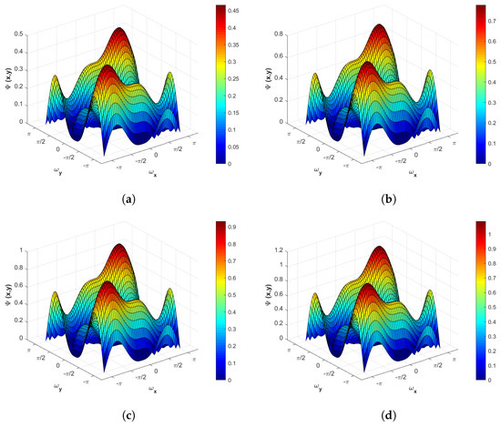
Figure 14. Plots of $\mathsf{\Psi }(x,y)$ vs. ${\omega }_x$ vs. ${\omega }_y$ for the $\Delta t$-values of $\Delta t=0.00008,0.0001,0.00012,0.00014$. (a) $\Delta t=0.00006$; (b) $\Delta t=0.00010$; (c) $\Delta t=0.00012$; (d) $\Delta t=0.00014$.

We deduce that the stability region is $|\Delta t|\le 0.00012.$

Remark 4. 

The above plot clearly shows that our numerical scheme in Equation (42) for the 2D KdV equation preserves stability for $\Delta t\le 0.00012$, as depicted in Figure 14, whereas, in Figure 14d, the instability behaviour emanates.

Consistency

We consider the dispersive 2D KdV equation given in Equation (9) and, using the Taylor series expansion about $(t_n,x_i,y_j),$ we have

$$\begin{array}{cc}\hfill U_t+U_{xxx}+U_{yyy}& =-\frac{{(\Delta t)}^2}{3!}{U}_{ttt}-\frac{{(\Delta t)}^4}{5!}{U}_{ttttt}-{\displaystyle \frac{30}{5!}}{(\Delta x)}^2{U}_{xxxxx}\hfill \\ & -{\displaystyle \frac{30}{5!}}{(\Delta y)}^2{U}_{yyyyy}+\mathcal{O}\left({(\Delta t)}^5\right)+\mathcal{O}\left({(\Delta x)}^3+{(\Delta y)}^3\right).\hfill \end{array}$$

Thus, the scheme in Equation (42) is consistent with the PDE in (9) and is second-order accurate in time and space.

Let us consider the homogeneous 2D-dispersive equation as in Equation (9) with $(t,x,y)\in [0,T]\times \mathsf{\Omega },T>0,\mathsf{\Omega }=[0,1]\times [0,1],$ subject to the initial condition in Equation (10); the time-dependent boundary conditions are given by

$$\left.\begin{array}{cc}\hfill u(t,x,0)=cos(2t+x),& u(t,x,1)=cos(1+2t+x),\hfill \\ \hfill u(t,0,y)=cos(2t+y),& u(t,1,y)=cos(2t+1+y),\hfill \end{array}\right\}$$

(48)

We note that the finite difference scheme given in Equation (42) works in such a way that the unknown value of $(i;j)$ at iteration $n+1$; $U_{i,j}^{n+1}$ is computed at the preceding $n^{th}$ iteration values of the indices $(i+1;j)$, $(i-1;j)$,$(i-2;j)$$(i;j)$, $(i;j+1)$, $(i;j-1)$, and $(i;j-2)$.

The initial condition in Equation (10) tells us that $u(0,x,y)=u_{i,j}^1=f(x_i,y_j)$ for $i=1,2,\dots ,\mathrm{N},$ while the non-zero Dirichlet boundary conditions in Equation (48) give the equations

$$\left.\begin{array}{cc}u(t_k,0,y_j)=u_{0,j}^k=cos(y_j+2t_k),\hfill & u(t_k,1,y_j)=u_{0,j}^k=cos(1+y_j+2t_k),\hfill \\ u(t_k,x_i,0)=u_{i,0}^k=cos(x_i+2t_k),\hfill & u(t_k,x_i,1)=u_{i,0}^k=cos(x_i+1+2t_k),\hfill \end{array}\right\}$$

for $i,j\in \left\{1,2,\dots ,\mathrm{N}\right\}$. In other words, if $(x_i,y_j)$ is a boundary node, then $u_{i,j}^n=g(x_i,y_j,t_k)$, where g is considered from the non-zero Dirichlet boundary conditions given in (48).

The following graphics depict plots of the maximum error vs. time and the loglog plot of the maximum error vs. time for numerical Experiment 3, as displayed in Figure 15.

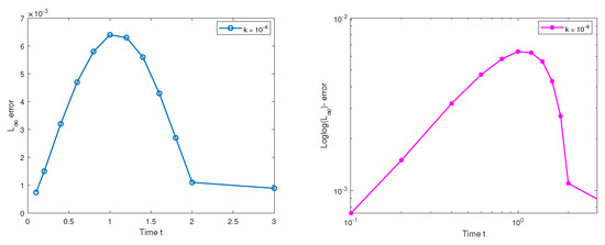
Figure 15. Plots of the maximum error vs. time $t\in [0,3.0]$ and the loglog plot of max. error vs. time using the standard FDM for Experiment 3 with $\Delta x=\Delta y=0.1$ and $\Delta t={10}^{-4}$.

Remark 5. 

When used to solve the homogeneous 2D KdV equation, VHPM performs excellently at $t=0.10$ and performs well at time $t=1.0$, but is less effective at time $t=2.0$. On the other hand, the classical finite difference scheme performs well for short, medium, and long time propagation, as shown in Table 3. We see that Figure 16 shows the 3D plots of the exact and numerical solution, using the standard finite difference scheme for Equation (42) on $\mathsf{\Omega }={(0,1)}^2$ at times $t=0.1,1.0,2.0$ with spatial step sizes $\Delta x=\Delta y=0.1$ and time step $\Delta t=0.0001$.

Table 3. A comparison between the exact solution and FDM solution at some values of x and y three different time propagations.

t	x	y	Exact Solution	FDM Solution	Absolute Error	Relative Error
	$0.0$	$0.0$	$9.800666\times {10}^{-1}$	$9.800666\times {10}^{-1}$	$0.00000$	$0.00000$
	$0.2$	$0.2$	$8.253356\times {10}^{-1}$	$8.256634\times {10}^{-1}$	$3.278350\times {10}^{-4}$	$3.972141\times {10}^{-4}$
		$0.4$	$6.967067\times {10}^{-1}$	$6.971658\times {10}^{-1}$	$4.591225\times {10}^{-4}$	$6.589897\times {10}^{-4}$
		$0.6$	$5.403023\times {10}^{-1}$	$5.408007\times {10}^{-1}$	$4.983545\times {10}^{-4}$	$9.223624\times {10}^{-4}$
		$0.8$	$3.623578\times {10}^{-1}$	$3.626549\times {10}^{-1}$	$2.971107\times {10}^{-4}$	$8.199376\times {10}^{-4}$
$0.10$	$0.4$	$0.2$	$6.967067\times {10}^{-1}$	$6.971658\times {10}^{-1}$	$4.591225\times {10}^{-4}$	$6.589897\times {10}^{-4}$
		$0.4$	$5.403023\times {10}^{-1}$	$5.410416\times {10}^{-1}$	$7.393096\times {10}^{-4}$	$1.368326\times {10}^{-3}$
		$0.6$	$3.623578\times {10}^{-1}$	$3.630982\times {10}^{-1}$	$7.404366\times {10}^{-4}$	$2.043385\times {10}^{-3}$
		$0.8$	$1.699671\times {10}^{-1}$	$1.704611\times {10}^{-1}$	$4.939410\times {10}^{-4}$	$2.906097\times {10}^{-3}$
	$0.6$	$0.2$	$5.403023\times {10}^{-1}$	$5.408007\times {10}^{-1}$	$4.983545\times {10}^{-4}$	$9.223624\times {10}^{-4}$
		$0.4$	$3.623578\times {10}^{-1}$	$3.630982\times {10}^{-1}$	$7.404366\times {10}^{-4}$	$2.043385\times {10}^{-3}$
		$0.6$	$1.699671\times {10}^{-1}$	$1.707071\times {10}^{-1}$	$7.399203\times {10}^{-4}$	$4.353314\times {10}^{-3}$
		$0.8$	$-2.919952\times {10}^{-2}$	$-2.874490\times {10}^{-2}$	$4.546532\times {10}^{-4}$	$1.557057\times {10}^{-2}$
	$0.8$	$0.2$	$3.623578\times {10}^{-1}$	$3.626549\times {10}^{-1}$	$2.971107\times {10}^{-4}$	$8.199376\times {10}^{-4}$
		$0.4$	$1.699671\times {10}^{-1}$	$1.704611\times {10}^{-1}$	$4.939410\times {10}^{-4}$	$2.906097\times {10}^{-3}$
		$0.6$	$2.919952\times {10}^{-2}$	$2.874487\times {10}^{-2}$	$4.546532\times {10}^{-4}$	$1.557057\times {10}^{-2}$
		$0.8$	$-2.272021\times {10}^{-1}$	$-2.268801\times {10}^{-1}$	$3.219550\times {10}^{-4}$	$1.417042\times {10}^{-3}$
	$1.0$	$1.0$	$-5.885011\times {10}^{-1}$	$-5.885011\times {10}^{-1}$	$0.000000$	$0.000000$
	$0.0$	$0.0$	$-4.161468\times {10}^{-1}$	$-4.161468\times {10}^{-1}$	$0.000000$	$0.000000$
	$0.2$	$0.2$	$-7.373937\times {10}^{-1}$	$-7.345692\times {10}^{-1}$	$2.824511\times {10}^{-3}$	$3.830398\times {10}^{-3}$
		$0.4$	$-8.568888\times {10}^{-1}$	$-8.529301\times {10}^{-1}$	$3.958671\times {10}^{-3}$	$4.619819\times {10}^{-3}$
		$0.6$	$-9.422223\times {10}^{-1}$	$-9.37927\times {10}^{-1}$	$4.295795\times {10}^{-3}$	$4.559216\times {10}^{-3}$
		$0.8$	$9.899925\times {10}^{-1}$	$-9.874045\times {10}^{-1}$	$2.588046\times {10}^{-3}$	$2.614208\times {10}^{-3}$
$1.0$	$0.4$	$0.2$	$-8.568888\times {10}^{-1}$	$-8.529301\times {10}^{-1}$	$3.958671\times {10}^{-3}$	$4.6198195\times {10}^{-3}$
		$0.4$	$-9.422223\times {10}^{-1}$	$-9.358445\times {10}^{-1}$	$6.377865\times {10}^{-3}$	$6.768959\times {10}^{-3}$
		$0.6$	$-9.8999249\times {10}^{-1}$	$-9.836041\times {10}^{-1}$	$6.388385\times {10}^{-3}$	$6.452963\times {10}^{-3}$
		$0.8$	$-9.982948\times {10}^{-1}$	$-9.939962\times {10}^{-1}$	$4.298589\times {10}^{-3}$	$4.305931\times {10}^{-3}$
	$0.6$	$0.2$	$-9.422223\times {10}^{-1}$	$-9.379265\times {10}^{-1}$	$4.295795\times {10}^{-3}$	$4.559216\times {10}^{-3}$
		$0.4$	$-9.899925\times {10}^{-1}$	$-9.836041\times {10}^{-1}$	$6.388385\times {10}^{-3}$	$6.452963\times {10}^{-3}$
		$0.6$	$-9.982948\times {10}^{-1}$	$-9.919138\times {10}^{-1}$	$6.381004\times {10}^{-3}$	$6.391904\times {10}^{-3}$
		$0.8$	$-9.667982\times {10}^{-1}$	$-9.628336\times {10}^{-1}$	$3.964556\times {10}^{-3}$	$4.100707\times {10}^{-3}$
	$0.8$	$0.2$	$-9.899925\times {10}^{-1}$	$-9.874045\times {10}^{-1}$	$2.588046\times {10}^{-3}$	$2.614208\times {10}^{-3}$
		$0.4$	$-9.982948\times {10}^{-1}$	$-9.939962\times {10}^{-1}$	$4.298589\times {10}^{-3}$	$4.305931\times {10}^{-3}$
		$0.6$	$-9.667982\times {10}^{-1}$	$-9.628336\times {10}^{-1}$	$3.964556\times {10}^{-3}$	$4.100707\times {10}^{-3}$
		$0.8$	$-8.967584\times {10}^{-1}$	$-8.939276\times {10}^{-1}$	$2.830849\times {10}^{-3}$	$3.156758\times {10}^{-3}$
	$1.0$	$1.0$	$6.536436\times {10}^{-1}$	$6.536436\times {10}^{-1}$	$0.000000$	$0.000000$
	$0.0$	$0.0$	$-6.536436\times {10}^{-1}$	$-6.536436\times {10}^{-1}$	$0.000000$	$0.000000$
	$0.2$	$0.2$	$-3.073329\times {10}^{-1}$	$-3.068653\times {10}^{-1}$	$4.675817\times {10}^{-4}$	$1.521418\times {10}^{-3}$
		$0.4$	$-1.121525\times {10}^{-1}$	$-1.114919\times {10}^{-1}$	$6.606069\times {10}^{-4}$	$5.890254\times {10}^{-3}$
		$0.6$	$8.749898\times {10}^{-2}$	$8.821557\times {10}^{-2}$	$7.165873\times {10}^{-4}$	$8.189664\times {10}^{-3}$
		$0.8$	$2.836622\times {10}^{-1}$	$2.840925\times {10}^{-1}$	$4.302832\times {10}^{-4}$	$1.516886\times {10}^{-3}$
$2.0$	$0.4$	$0.2$	$-1.121525\times {10}^{-1}$	$-1.114919\times {10}^{-1}$	$6.606069\times {10}^{-4}$	$5.890254\times {10}^{-3}$
		$0.4$	$8.749898\times {10}^{-2}$	$8.857237\times {10}^{-2}$	$1.073386\times {10}^{-3}$	$1.226741\times {10}^{-2}$
		$0.6$	$2.836622\times {10}^{-1}$	$2.847349\times {10}^{-1}$	$1.072748\times {10}^{-3}$	$3.781779\times {10}^{-3}$
		$0.8$	$4.685167\times {10}^{-1}$	$4.692368\times {10}^{-1}$	$7.201221\times {10}^{-4}$	$1.537025\times {10}^{-3}$
	$0.6$	$0.2$	$8.749898\times {10}^{-2}$	$8.821557\times {10}^{-2}$	$7.165873\times {10}^{-4}$	$8.189664\times {10}^{-3}$
		$0.4$	$2.836622\times {10}^{-1}$	$2.847349\times {10}^{-1}$	$1.072748\times {10}^{-3}$	$3.781779\times {10}^{-3}$
		$0.6$	$4.685167\times {10}^{-1}$	$4.695865\times {10}^{-1}$	$1.069798\times {10}^{-3}$	$2.283372\times {10}^{-3}$
		$0.8$	$6.346929\times {10}^{-1}$	$6.353552\times {10}^{-1}$	$6.6228012\times {10}^{-4}$	$1.043466\times {10}^{-3}$
	$0.8$	$0.2$	$2.836622\times {10}^{-1}$	$2.840925\times {10}^{-1}$	$4.302832\times {10}^{-4}$	$1.516886\times {10}^{-3}$
		$0.4$	$4.685167\times {10}^{-1}$	$4.692368\times {10}^{-1}$	$7.201221\times {10}^{-4}$	$1.537025\times {10}^{-3}$
		$0.6$	$6.346929\times {10}^{-1}$	$6.353552\times {10}^{-1}$	$6.622802\times {10}^{-4}$	$1.043466\times {10}^{-3}$
		$0.8$	$7.755659\times {10}^{-2}$	$7.760373\times {10}^{-2}$	$4.713753\times {10}^{-4}$	$6.077824\times {10}^{-4}$
	$1.0$	$1.0$	$9.601703\times {10}^{-1}$	$9.601703\times {10}^{-1}$	$0.000000$	$0.000000$

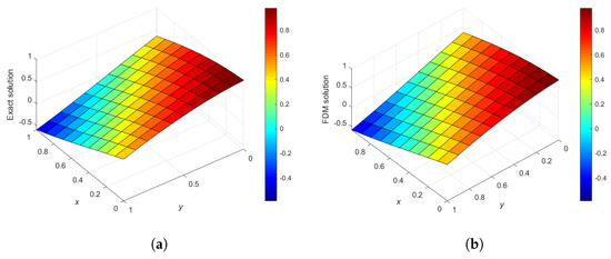
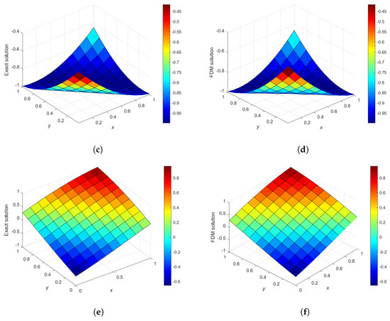
Figure 16. Plots of exact and numerical solution vs. x vs. y, using the classical FDMscheme of Equation (42) on $\mathsf{\Omega }={(0,1)}^2$ at t = 0.10, 1.0, 2.0 used spatial step sizes Δx = Δy = 0.1 and time-step Δt = 0.0001. (a) Time = 0.10; (b) Time = 0.10; (c) Time = 1.0; (d) Time = 1.0; (e) Time = 2.0; (f) Time = 2.0.

7. Numerical Experiment 4

7.1. Solution of Numerical Experiment 4 Using VHPM

Let us consider the non-homogeneous 2D KdV equation given in Equation (12). We now apply the VHPM procedure given in Equations (3) and (5) into Equation (12) to obtain

$$\sum _{i=0}^{\infty }{\rho }^i{u}_i(t,x)=u_0(t,x)+\rho \left[{\int }_0^t\lambda \left(\tau \right)\left\{\mathcal{L}\left(\sum _{i=0}^{\infty }{\rho }^i{u}_i\right)+\mathcal{N}\left(\sum _{i=0}^{\infty }{\rho }^i{\tilde{u}}_i\right)\right\}\mathrm{d}\tau -{\int }_0^t\lambda \left(\tau \right)g(\tau ,x)\mathrm{d}\tau \right].$$

(49)

Equation (49) reduces to

$$\sum _{i=0}^{\infty }{\rho }^i{u}_i(t,x)=u_0(t,x)-\rho \left({\int }_0^t\left({\displaystyle \sum _{n=0}^{\infty }{\rho }^n{u}_{n,xxx}+\sum _{n=0}^{\infty }{\rho }^n{u}_{n,yyy}-g(x,\tau )}\right)\mathrm{d}\tau \right),$$

(50)

where the source term is $g(t,x)=e^{t}cos(x-y)$.

By now collecting terms of the same power of $\rho$, the components of $u_i$’s are obtained as

$$\left.\begin{array}{cc}\hfill {\rho }^{\left(0\right)}:& u_0(x,y)=cos(x-y),\hfill \\ \hfill {\rho }^{\left(1\right)}:& u_1(t,x,y)=-{\int }_0^t\left(u_{0,xxx}(\tau ,x,y)+u_{0,yyy}(\tau ,x,y)-g(x,\tau )\right)\mathrm{d}\tau \hfill \\ \hfill {\rho }^{\left(2\right)}:& u_2(t,x,y)=-{\int }_0^t\left(u_{1,xxx}(\tau ,x,y)+u_{1,yyy}(\tau ,x,y)\right)\mathrm{d}\tau \hfill \\ \hfill {\rho }^{\left(n\right)}:& u_n(t,x,y)=-{\int }_0^t\left(u_{n-1,xxx}(\tau ,x,y)+u_{n-1,yyy}(\tau ,x,y)\right)\mathrm{d}\tau ,n\ge 3.\hfill \end{array}\right\}$$

(51)

Using Equation (51), the solution, using VHPM, reads as

$$\left.\begin{array}{c}{u}_0(x,y)=cos(x-y),\hfill \\ u_1(t,x,y)=e^{t}cos(x-y)-cos(x-y),\hfill \\ u_n(t,x,y)=0,n\ge 2.\hfill \end{array}\right\}$$

(52)

By looking at the components $u_0$ and $u_1$ in Equation (52), one can easily observe that the first two terms are self-cancelling (noise) terms, confirming that the exact solution is concentrated in the initial few approximations. It is of note that the higher-order components vanish quickly to assure rapid convergence to the exact solution. Figure 17 shows the 3D plots of the exact and VHPM solution vs. x vs. y for Experiment 4.

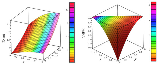
Figure 17. (Left) Graphical representation of the exact (as well as the VHPM) solution vs. $x\in [0,1.0]$ vs. $t\in [0,1.0]$ along $y=0.95$, and (Right) plot of the VHPM solution (with $n=2$) (as well as the exact solution) vs. $x\in [0,1.0]$ vs. $y\in [0,1.0]$ at time $t=0.50$.

Remark 6. 

Following the approaches described in [27,46,47], if we modify VHPM by shifting the source term, we obtain a solution which converges to the exact solution after only two iterations. Such a modification for most PDEs usually gives a promising result, depending on the type of problem considered (cf. [48]). We note here that G. Adomian and Rach [49] and Wazwaz [45] investigated the phenomenon of self-cancelling ‘noise’ terms where some terms in the series vanish on the limit. These ‘noise’ terms do not show up for homogeneous equations but solely for specific types of non-homogeneous equations. It was formally shown that by cancelling the noise terms that appear in $u_0$ and $u_1$ from $u_0$, even though $u_1$ contains additional terms, the remaining non-cancelled terms of $u_0$ may give the exact solution of the non-homogeneous problem [43].

7.2. Solution of Numerical Experiment 4 Using Finite Difference Scheme

To obtain the stability region of the classical FDM for Experiment 4, we consider the following scheme

$$\begin{array}{cc}\hfill U_{i,j}^{n+1}& =U_{i,j}^{n-1}-r_x\left(U_{i+2,j}^n-2U_{i+1,j}^n+2U_{i-1,j}^n-U_{i-2,j}^n\right)\hfill \\ & -r_y\left(U_{i,j+2}^n-2U_{i,j+1}^n+2U_{i,j-1}^n-U_{i,j-2}^n\right)-2\Delta t\left(exp\left(t_n\right)cos(x_i-y_j)\right),\hfill \end{array}$$

(53)

where $r_x$ and $r_y$ are given in Equation (43).

Taylor’s series expansion about $(t_n,x_i,y_j)$ gives

$$\begin{array}{cc}\hfill U+(\Delta t)U_t& +\frac{{(\Delta t)}^2}{2!}{U}_{tt}+\frac{{(\Delta t)}^3}{3!}{U}_{ttt}+\frac{{(\Delta t)}^4}{4!}{U}_{tttt}+\frac{{(\Delta t)}^5}{5!}{U}_{ttttt}+\mathcal{O}\left({(\Delta t)}^6\right)\hfill \\ & =U-(\Delta t)U_t+\frac{{(\Delta t)}^2}{2!}{U}_{tt}-\frac{{(\Delta t)}^3}{3!}{U}_{ttt}+\frac{{(\Delta t)}^4}{4!}{U}_{tttt}-\frac{{(\Delta t)}^5}{5!}{U}_{ttttt}+\mathcal{O}\left({(\Delta t)}^6\right)-2(\Delta t)\left(exp\left(t_n\right)cos(x_i-y_j)\right)\hfill \\ \hfill & -\frac{(\Delta t)}{{(\Delta x)}^3}\left[2{(\Delta x)}^3{U}_{xxx}+{\displaystyle \frac{60}{5!}}{(\Delta x)}^5{U}_{xxxxx}+\mathcal{O}\left({(\Delta x)}^6\right)\right]-\frac{(\Delta t)}{{(\Delta y)}^3}\left[2{(\Delta y)}^3{U}_{yyy}+{\displaystyle \frac{60}{5!}}{(\Delta y)}^5{U}_{yyyyy}+\mathcal{O}\left({(\Delta y)}^6\right)\right].\hfill \end{array}$$

(54)

Simplifying Equation (54) gives

$$\begin{array}{cc}\hfill U_t+U_{xxx}+U_{yyy}-exp\left(t\right)cos(x-y)& =-\frac{{(\Delta t)}^2}{3!}{U}_{ttt}-\frac{{(\Delta t)}^4}{5!}{U}_{ttttt}-{\displaystyle \frac{30}{5!}}{(\Delta x)}^2{U}_{xxxxx}\hfill \\ & -{\displaystyle \frac{30}{5!}}{(\Delta y)}^2{U}_{yyyyy}+\mathcal{O}\left({(\Delta t)}^5\right)+\mathcal{O}\left({(\Delta x)}^3+{(\Delta y)}^3\right).\hfill \end{array}$$

Thus, the scheme is consistent with the PDE in (12) and is second-order accurate in time and space.

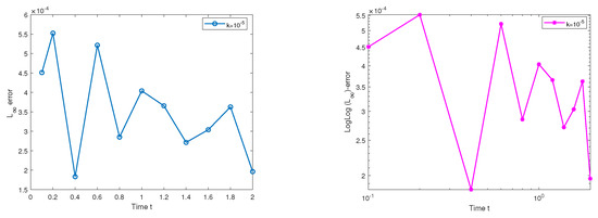
Figure 18 shows plots of the maximum error vs. time and the loglog plot of the maximum error vs. time using the classical FDM for Experiment 4.

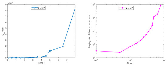
Figure 18. Plots for the maximum error vs. time $t\in [0,8.0]$ and the loglog plot of the max. error vs. time using the standard FDM for Experiment 4 with $\Delta x=\Delta y=0.1$ and $\Delta t={10}^{-4}$, respectively.

Figure 19 gives the 3D plots for the numerical solution vs. x vs. y, using the classical FDM with the exact solution at times $t=1.0,2.0,5.0,8.0$ for Experiment 4. We can also see from Table 4 that the classical finite difference scheme performs very well for numerical Experiment 4 and that the numerical results using VHPM rapidly converge to the exact solution, as shown in Section 7.1.

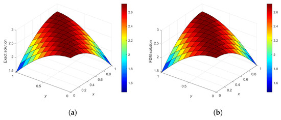
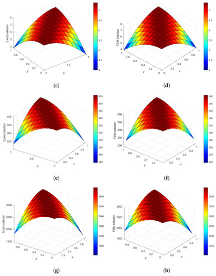
Figure 19. 3D plots of the exact and the FDM solution vs. x vs. y for (x;y) ∈ Ω, Ω = ${(0,1)}^2$ (Δt = ${10}^{-4}$) at times t = 1.0, 2.0, 5.0, 8.0. (a) Δt = 1.0 $\times {10}^{-4}$, Time = 1.0; (b) Δt = 1.0 $\times {10}^{-4}$, Time = 1.0; (c) Δt = 1.0 $\times {10}^{-4}$, Time = 2.0; (d) Δt = 1.0 $\times {10}^{-4}$, Time = 2.0; (e) Δt = 1.0 $\times {10}^{-4}$, Time = 5.0; (f) Δt = 1.0 $\times {10}^{-4}$, Time = 5.0; (g) Δt = 1.0 $\times {10}^{-4}$, Time = 8.0; (h) Δt = 1.0 $\times {10}^{-4}$, Time = 8.0.

Table 4. A comparison between the exact solution and FDM solution at some values of x and y at times $t=0.10,1.0,2.0$ (Experiment 4).

t	x	y	Exact Solution	FDM Solution	Absolute Error	Relative Error
	$0.0$	$0.0$	$1.105171$	$1.105171$	$0.000000$	$0.000000$
	$0.2$	$0.2$	$1.105171$	$1.105171$	$3.272759\times {10}^{-9}$	$2.961315\times {10}^{-9}$
		$0.4$	$1.083141$	$1.083141$	$1.980772\times {10}^{-9}$	$1.828729\times {10}^{-9}$
		$0.6$	$1.017929$	$1.017929$	$2.657259\times {10}^{-9}$	$2.610454\times {10}^{-9}$
		$0.8$	$9.121369\times {10}^{-1}$	$9.121369\times {10}^{-1}$	$1.202890\times {10}^{-10}$	$1.318760\times {10}^{-10}$
$0.10$	$0.4$	$0.2$	$1.083141$	$1.083141$	$1.980772\times {10}^{-9}$	$1.828729\times {10}^{-9}$
		$0.4$	$1.105171$	$1.105171$	$1.898155\times {10}^{-10}$	$1.717522\times {10}^{-10}$
		$0.6$	$1.083141$	$1.083141$	$2.864586\times {10}^{-10}$	$2.644703\times {10}^{-10}$
		$0.8$	$1.017929$	$1.017929$	$2.278236\times {10}^{-9}$	$2.238107\times {10}^{-9}$
	$0.8$	$0.2$	$9.121377\times {10}^{-1}$	$9.121369\times {10}^{-1}$	$1.202870\times {10}^{-10}$	$1.318738\times {10}^{-10}$
		$0.4$	$1.017930$	$1.017929$	$2.278236\times {10}^{-9}$	$2.238107\times {10}^{-9}$
		$0.6$	$1.083141$	$1.083141$	$1.605688\times {10}^{-9}$	$1.482437\times {10}^{-9}$
		$0.8$	$1.105171$	$1.105171$	$2.971336\times {10}^{-9}$	$2.688576\times {10}^{-9}$
	$1.0$	$1.0$	$1.105171$	$1.105171$	$0.000000$	$0.000000$
	$0.0$	$0.0$	$2.718282$	$2.718282$	$0.000000$	$0.000000$
	$0.2$	$0.2$	$2.718282$	$2.718282$	$1.049272\times {10}^{-9}$	$3.860057\times {10}^{-10}$
		$0.4$	$2.664097$	$2.664097$	$2.499563\times {10}^{-9}$	$9.382401\times {10}^{-10}$
		$0.6$	$2.503703$	$2.503703$	$1.876913\times {10}^{-9}$	$7.496546\times {10}^{-10}$
		$0.8$	$2.243495$	$2.243495$	$1.960433\times {10}^{-9}$	$8.738300\times {10}^{-10}$
$1.0$	$0.4$	$0.2$	$2.664097$	$2.664097$	$2.499576\times {10}^{-9}$	$9.382449\times {10}^{-10}$
		$0.4$	$2.718282$	$2.718282$	$6.650187\times {10}^{-9}$	$2.446467\times {10}^{-9}$
		$0.6$	$2.664097$	$2.664097$	$4.694272\times {10}^{-9}$	$1.762050\times {10}^{-9}$
		$0.8$	$2.503703$	$2.503703$	$4.319871\times {10}^{-9}$	$1.725393\times {10}^{-9}$
	$0.8$	$0.2$	$2.243495$	$2.243495$	$1.960426\times {10}^{-9}$	$8.738269\times {10}^{-10}$
		$0.4$	$2.503703$	$2.503703$	$4.319886\times {10}^{-9}$	$1.725398\times {10}^{-9}$
		$0.6$	$2.664097$	$2.664097$	$3.635933\times {10}^{-9}$	$1.364789\times {10}^{-9}$
		$0.8$	$2.718282$	$2.718282$	$3.871336\times {10}^{-9}$	$1.424185\times {10}^{-9}$
	$1.0$	$1.0$	$2.718282$	$2.718282$	$0.000000$	$0.000000$
	$0.2$	$0.2$	$7.389056$	$7.389056$	$6.118424\times {10}^{-9}$	$8.280386\times {10}^{-10}$
		$0.4$	$7.241767$	$7.241767$	$9.911319\times {10}^{-9}$	$1.368633\times {10}^{-9}$
		$0.6$	$6.805771$	$6.805771$	$9.219519\times {10}^{-9}$	$1.354662\times {10}^{-9}$
		$0.8$	$6.098451$	$6.098451$	$7.290955\times {10}^{-9}$	$1.195542\times {10}^{-9}$
$2.0$	$0.4$	$0.2$	$7.241767$	$7.241767$	$9.911327\times {10}^{-9}$	$1.368634\times {10}^{-9}$
		$0.4$	$7.389056$	$7.389056$	$1.911231\times {10}^{-8}$	$2.586570\times {10}^{-9}$
		$0.6$	$7.241767$	$7.241767$	$1.745360\times {10}^{-8}$	$2.410131\times {10}^{-9}$
		$0.8$	$6.805771$	$6.805771$	$1.382399\times {10}^{-8}$	$2.031217\times {10}^{-9}$
	$0.8$	$0.2$	$6.098451$	$6.098451$	$7.290940\times {10}^{-9}$	$1.1955397\times {10}^{-9}$
		$0.4$	$6.805771$	$6.805771$	$1.382399\times {10}^{-8}$	$2.031217\times {10}^{-9}$
		$0.6$	$7.241767$	$7.241767$	$1.290455\times {10}^{-8}$	$1.781962\times {10}^{-9}$
		$0.8$	$7.389056$	$7.389056$	$1.218180\times {10}^{-8}$	$1.648628\times {10}^{-9}$
	$1.0$	$1.0$	$7.389056$	$7.389056$	$0.000000$	$0.000000$
	$0.0$	$0.0$	$2.980958\times {10}^3$	$2.980958\times {10}^3$	$0.000000$	$0.000000$
	$0.2$	$0.2$	$2.980958\times {10}^3$	$2.980958\times {10}^3$	$4.273845\times {10}^{-6}$	$1.433715\times {10}^{-9}$
		$0.4$	$2.921537\times {10}^3$	$2.9215370\times {10}^3$	$5.325453\times {10}^{-6}$	$1.822825\times {10}^{-9}$
		$0.6$	$2.745644\times {10}^3$	$2.745644\times {10}^3$	$5.379429\times {10}^{-6}$	$1.959259\times {10}^{-9}$
		$0.8$	$2.460291\times {10}^3$	$2.460291\times {10}^3$	$3.400780\times {10}^{-6}$	$1.382268\times {10}^{-9}$
$8.0$	$0.4$	$0.2$	$2.921537\times {10}^3$	$2.921537\times {10}^3$	$5.325440\times {10}^{-6}$	$1.822821\times {10}^{-9}$
		$0.4$	$2.980958\times {10}^3$	$2.980958\times {10}^3$	$8.472980\times {10}^{-6}$	$2.842368\times {10}^{-9}$
		$0.6$	$2.921537\times {10}^3$	$2.921537\times {10}^3$	$8.140318\times {10}^{-6}$	$2.786313\times {10}^{-9}$
		$0.8$	$2.745644\times {10}^3$	$2.745644\times {10}^3$	$5.368224\times {10}^{-6}$	$1.955178\times {10}^{-9}$
	$0.8$	$0.2$	$2.460291\times {10}^3$	$2.460291\times {10}^3$	$3.400739\times {10}^{-6}$	$1.382251\times {10}^{-9}$
		$0.4$	$2.745644\times {10}^3$	$2.745644\times {10}^3$	$5.368230\times {10}^{-6}$	$1.955181\times {10}^{-9}$
		$0.6$	$2.921537\times {10}^3$	$2.921537\times {10}^3$	$5.316034\times {10}^{-6}$	$1.819602\times {10}^{-9}$
		$0.8$	$2.980958\times {10}^3$	$2.980958\times {10}^3$	$4.261710\times {10}^{-6}$	$1.429644\times {10}^{-9}$
	$1.0$	$1.0$	$2.980958\times {10}^3$	$2.980958\times {10}^3$	$0.000000$	$0.000000$

8. Numerical Experiment 5

8.1. Solution of Numerical Experiment 5 Using VHPM

Let us now rewrite Equation (42) as

$$\mathcal{L}u+\mathcal{M}u+\mathcal{N}u=0,$$

where the differential operators are given by $\mathcal{L}={\displaystyle \frac{\partial }{\partial t}}$ and $\mathcal{M}=-{\displaystyle \frac{{\partial }^3}{\partial x^3}}$ and $\mathcal{N}=-3{\left({\displaystyle \frac{\partial }{\partial x}}\right)}^2$.

Using Equation (5), we write Equation (42) as

$$\sum _{i=0}^{\infty }{\rho }^i{u}_i(t,x)=u_0(t,x)-\rho \left[{\int }_0^t\left\{\left(3{\left(\sum _{n=0}^{\infty }{\rho }^i{u}_{n,x}\right)}^2+\sum _{n=0}^{\infty }{\rho }^i{u}_{n,xxx}\right)\right\}\mathrm{d}\tau \right],$$

(55)

where $u_{i,x}={\displaystyle \frac{\partial u_i(t,x)}{\partial x}}$ and $u_{i,xxx}={\displaystyle \frac{{\partial }^3{u}_i(t,x)}{\partial x^3}}$. By comparing like terms of $\rho$ on both sides of Equation (17), we obtain the following components:

$$\left.\begin{array}{ccc}{\rho }^{\left(0\right)}:\hfill & u_0\left(x\right)\hfill & =\frac{1}{2}{sech}^2\left(\frac{1}{2}x\right),\hfill \\ {\rho }^{\left(1\right)}:\hfill & u_1(t,x)\hfill & =-{\int }_0^t\left(6u_0{u}_{0,x}(\tau ,x)+u_{0,xxx}(\tau ,x)\right)\mathrm{d}\tau =\frac{1}{2}\frac{sinh\left(\frac{x}{2}\right)t}{{\left(cosh\left(\frac{x}{2}\right)\right)}^3},\hfill \\ {\rho }^{\left(2\right)}:\hfill & u_2(t,x)\hfill & =-{\int }_0^t\left[3{\left(2u_0{u}_1\right)}_x+u_{1,xxx}(\tau ,x)\right]\mathrm{d}\tau =\frac{1}{8}\frac{\left(2{\left(cosh\left(\frac{x}{2}\right)\right)}^2-3\right)t^2}{{\left(cosh\left(\frac{x}{2}\right)\right)}^4}\hfill \\ {\rho }^{\left(3\right)}:\hfill & u_3(t,x)\hfill & {\displaystyle =-{\int }_0^t\left[\left(3{\left(u_1^2+2u_0{u}_2\right)}_x\right)+\left(u_{2,xxx}(\tau ,x)\right)\right]\mathrm{d}\tau =\frac{1}{12}\frac{sinh\left(\frac{x}{2}\right)\left({\left(cosh\left(\frac{x}{2}\right)\right)}^2-3\right)t^3}{{\left(cosh\left(\frac{x}{2}\right)\right)}^5},}\hfill \\ {\rho }^{\left(4\right)}:\hfill & u_4(t,x)\hfill & {\displaystyle =-{\int }_0^t\left[3\left({\left(2u_1{u}_2\right)}_x+{\left(2u_0{u}_3\right)}_x+{\left(2u_1{u}_2\right)}_x\right)+u_{2,xxx}(\tau ,x)\right]\mathrm{d}\tau }\hfill \\ & & =\frac{\left(4{\left(cosh\left(\frac{x}{2}\right)\right)}^6+42{\left(cosh\left(\frac{x}{2}\right)\right)}^4-222{\left(cosh\left(\frac{x}{2}\right)\right)}^2+189\right)t^4}{192{\left(cosh\left(\frac{x}{2}\right)\right)}^8}.\hfill \end{array}\right\}$$

(56)

Thus, the sum of the first five-term approximate solution obtained by VHPM in Equation (56) takes the form

$$\begin{array}{cc}\hfill {\mathcal{S}}_4(x,t)& =\frac{\left(4{\left(cosh\left(\frac{x}{2}\right)\right)}^6+42{\left(cosh\left(\frac{x}{2}\right)\right)}^4-222{\left(cosh\left(\frac{x}{2}\right)\right)}^2+189\right)t^4}{192{\left(cosh\left(\frac{x}{2}\right)\right)}^8}+\frac{1}{2}\frac{sinh\left(\frac{x}{2}\right)t}{{\left(cosh\left(\frac{x}{2}\right)\right)}^3}+\frac{1}{2}{\left(cosh\left(\frac{x}{2}\right)\right)}^{-2}\hfill \\ & +\frac{\left(16{\left(cosh\left(\frac{x}{2}\right)\right)}^{5}sinh\left(\frac{x}{2}\right)-48{\left(cosh\left(\frac{x}{2}\right)\right)}^{3}sinh\left(\frac{x}{2}\right)\right)t^3}{192{\left(cosh\left(\frac{x}{2}\right)\right)}^8}+\frac{\left(48{\left(cosh\left(\frac{x}{2}\right)\right)}^6-72{\left(cosh\left(\frac{x}{2}\right)\right)}^4\right)t^2}{192{\left(cosh\left(\frac{x}{2}\right)\right)}^8}.\hfill \end{array}$$

In Table 5, the absolute and relative errors are tabulated for some values of x at four different time values: $0.01,0.5,1.0$, and $2.0$. Figure 20 displays graphically the exact and the VHPM solutions to Experiment 5.

Table 5. Absolute and relative errors (VHPM with $n=4$) at some values of $x\in [0,2\pi ]$ and $t\in [0,2.0]$.

x	t	Exact Solution	VHPM Solution	Absolute Error	Relative Error
	0.01	0.4317811	0.4317811	1.899052 $\times {10}^{-10}$	4.398183 $\times {10}^{-10}$
$\frac{\pi }{4}$	0.5	0.4899551	0.4885655	1.389585 $\times {10}^{-3}$	2.836147 $\times {10}^{-3}$
	1.0	0.4942872	0.4689259	2.536130 $\times {10}^{-2}$	5.130883 $\times {10}^{-2}$
	2.0	0.3529964	−0.1116201	4.646165 $\times {10}^{-1}$	1.316208 $\times {10}^0$
	0.01	0.2868378	0.2868378	1.730594 $\times {10}^{-10}$	6.033353 $\times {10}^{-10}$
$\frac{\pi }{2}$	0.5	0.3801965	0.3791079	1.088588$\times {10}^{-3}$	2.863224 $\times {10}^{-3}$
	1.0	0.4613875	0.4431495	1.823802 $\times {10}^{-2}$	3.952863 $\times {10}^{-2}$
	2.0	0.4776620	0.1283443	3.493177 $\times {10}^{-1}$	7.313072 $\times {10}^{-1}$
	0.01	0.0801472	0.0801472	4.832666 $\times {10}^{-11}$	6.029739 $\times {10}^{-10}$
$\pi$	0.5	0.1241713	0.1244916	3.203225 $\times {10}^{-4}$	2.579683 $\times {10}^{-3}$
	1.0	0.1881387	0.1936758	5.537052 $\times {10}^{-3}$	2.943068 $\times {10}^{-2}$
	2.0	0.3669010	0.4740549	1.071540 $\times {10}^{-1}$	2.920515 $\times {10}^{-1}$
	0.01	0.0178223	0.0178223	4.102757 $\times {10}^{-12}$	2.302041 $\times {10}^{-10}$
$\frac{3\pi }{2}$	0.5	0.0287635	0.0287870	2.345761 $\times {10}^{-5}$	8.155326 $\times {10}^{-4}$
	1.0	0.0465377	0.0468804	3.427113 $\times {10}^{-4}$	7.364171 $\times {10}^{-3}$
	2.0	0.1167433	0.1217444	5.001064 $\times {10}^{-3}$	4.283812$\times {10}^{-2}$
	0.01	0.0082059	0.0082059	9.294671 $\times {10}^{-13}$	1.132676 $\times {10}^{-10}$
$\frac{7\pi }{4}$	0.5	0.0133252	0.0133293	4.150761 $\times {10}^{-6}$	3.114977$\times {10}^{-4}$
	1.0	0.0217795	0.0218161	3.658641 $\times {10}^{-5}$	1.679852 $\times {10}^{-3}$
	2.0	0.0570247	0.0565798	4.449361 $\times {10}^{-4}$	7.802514 $\times {10}^{-3}$
	0.01	0.0037582	0.0037582	1.995532 $\times {10}^{-13}$	5.309766$\times {10}^{-11}$
$2\pi$	0.5	0.0061200	0.0061204	3.401180 $\times {10}^{-7}$	5.557447 $\times {10}^{-5}$
	1.0	0.0100502	0.0100385	1.164189 $\times {10}^{-5}$	1.158376 $\times {10}^{-3}$
	2.0	0.0268511	0.0259934	8.577236 $\times {10}^{-4}$	3.194365 $\times {10}^{-2}$

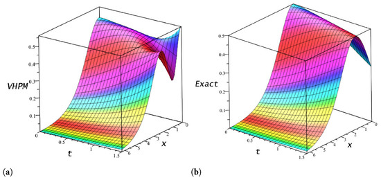
Figure 20. 3D plot of the exact and approximate solutions, using $n=4$ terms from VHPM vs. $x\in [0,2\pi ]$ vs. $t\in [0,1.5]$. (a) Solution using VHPM; (b) Exact solution.

8.2. Solution of Numerical Experiment 5 Using Finite Difference Scheme

Let us consider Equation (42). Equation (18) is discretised, using the Zabusky–Kruskal method [9], as

$$\begin{array}{c}\hfill \frac{U_i^{n+1}-U_i^{n-1}}{2\Delta t}=-6\left(\frac{U_{i-1}^n+U_i^n+U_{i+1}^n}{3}\right)\left(\frac{U_{i+1}^n-U_{i-1}^n}{2\Delta x}\right)-\left(\frac{U_{i+2}^n-2U_{i+1}^n+2U_{i-1}^n-U_{i-2}^n}{2{(\Delta x)}^3}\right).\end{array}$$

(57)

The scheme is given by

$$\begin{array}{c}\hfill U_i^{n+1}=U_i^{n-1}-{\displaystyle \frac{2·\Delta t}{\Delta x}}·\left(U_{i-1}^n+U_i^n+U_{i+1}^n\right)\left(U_{i+1}^n-U_{i-1}^n\right)-{\displaystyle \frac{\Delta t}{{(\Delta x)}^3}}·\left(U_{i+2}^n-2U_{i+1}^n+2U_{i-1}^n-U_{i-2}^n\right),\end{array}$$

(58)

for $i=3,4,\dots ,\mathrm{N}-1$ and $n=2,3,\dots ,\mathrm{Itmax}-1$. To facilitate the numerical computation, we need to use another scheme to obtain a solution at the second time level by proposing the following scheme:

$$\begin{array}{c}\hfill U_j^2=U_j^1-{\displaystyle \frac{(\Delta t)}{\Delta x}}\left(U_{j-1}^1+U_j^1+U_{j+1}^1\right)\left(U_{j+1}^1-U_{j-1}^1\right)-{\displaystyle \frac{(\Delta t)}{2{(\Delta x)}^3}}\left(U_{j+2}^1-2U_{j+1}^1+2U_{j-1}^1-U_{j-2}^1\right),\end{array}$$

for $i=3,4,\dots ,\mathrm{N}-1$ and $n=2,3,\dots ,\mathrm{Itmax}-1$.

The stability region of the scheme for Equation (14) can be determined by relying on the idea of frozen coefficients [50] for writing $u{u}_x$ as $u_{\max }{u}_x$, together with the von Neumann ansatz

$$U_j^n={\xi }^n{e}^{Ij\omega },$$

where $\omega =\theta h$ is the phase angle, to obtain the following relation from Equation (58),

$$\begin{array}{c}\hfill {\xi }^2+\mathcal{K}\xi -1=0,\end{array}$$

(59)

where

$$\left.\begin{array}{c}\mathcal{K}=\left(12u_{\max }\lambda Isin\left(\omega \right)\right)+\frac{\lambda }{{(\Delta x)}^2}\left(2Isin\left(2\omega \right)-4Isin\left(\omega \right)\right),\hfill \\ \lambda =\frac{\Delta t}{\Delta x},\mathrm{and}I=\sqrt{-1}\hfill \end{array}\right\}$$

(60)

, with $u_{\max }$ the least upper bound on $\left|u\right(x,t\left)\right|$.

Solving Equation (59) gives

$$\begin{array}{c}\hfill \xi ={\displaystyle \frac{-\mathcal{K}\pm \sqrt{{\mathcal{K}}^2+4}}{2}}\end{array}$$

(61)

where $\mathcal{K}$ is given in Equation (60).

A condition for the stability criterion is obtained by finding a condition on $\Delta t,\Delta x$ so that, for $\omega \in [-\pi ,\pi ]$, $\left|\xi \right|\le 1$ is true. This gives

$$\begin{array}{c}\hfill 4-{\left(12\lambda ·|u_{\max }|(Isin\left(\omega \right))+{\displaystyle \frac{\lambda }{{(\Delta x)}^2}}·\left(2Isin\left(2\omega \right)-4Isin\left(\omega \right)\right)\right)}^2\ge 0,\end{array}$$

which gives

$$\begin{array}{c}\hfill |6\lambda ·|u_{\max }|(Isin\left(\omega \right))+{\displaystyle \frac{\lambda }{{(\Delta x)}^2}}·\left(Isin\left(2\omega \right)-2Isin\left(\omega \right)\right)|\le 1.\end{array}$$

(62)

Since the second expression in the bracket for the above inequality dominates the first for small values of $\Delta x$, we obtain $\omega =\frac{2\pi }{3}$ from the second expression, which gives the maximum value for the inequality.

On substituting this into the inequality, we obtain the region of stability as [51]

$$\begin{array}{c}\hfill \left|\lambda \right|\le {\displaystyle \frac{1}{\left|\right\{6u_{\max }sin\left(2\omega \right)+\frac{1}{{(\Delta x)}^2}\left(sin\left(2\omega \right)-2sin\left(\omega \right)\right)\left\}\right|}}\le \left|{\displaystyle \frac{1}{3\sqrt{3}{u}_{\max }-\frac{3\sqrt{3}}{2{(\Delta x)}^2}}}\right|=\left|{\displaystyle \frac{1}{3\sqrt{3}(u_{\max }-\frac{1}{2{(\Delta x)}^2})}}\right|.\end{array}$$

(63)

By considering $\Delta x=\frac{\pi }{10}$ with $u_{max}\approx 0.50$ (using the Maple max function) for $x\in [0,2\pi ]$, Equation (63) gives

$$\begin{array}{c}\hfill 0<\Delta t\le \left|{\displaystyle \frac{\frac{\pi }{10}}{\frac{3\sqrt{3}}{2}-\frac{3\sqrt{3}}{2}\left(\frac{100}{{\pi }^2}\right)}}\right|=0.04214796.\end{array}$$

(64)

Equation (64) is the stability region of the scheme in Equation (58) for $\Delta x=\frac{\pi }{10}.$

Consistency of the Numerical Scheme in Equation (42)

We consider Equation (42). The Taylor series expansion about $(t_n,x_i)$ gives

$$\begin{array}{c}\hfill U_t+6U{U}_x+U_{xxx}=-{\displaystyle \frac{{(\Delta t)}^2}{3}}{U}_{ttt}+\frac{3{(\Delta x)}^2}{2}{U}_{xxxxx}+2{(\Delta x)}^2{U}_x{U}_{xxx}+\frac{{(\Delta x)}^4}{3}{U}_{xx}{U}_{xxxx}+\dots \end{array}$$

(65)

The scheme is consistent with the PDE given in Equation (42) and is second-order accurate in time and space.

The following are plots of the numerical and exact profiles vs. x in Figure 21, Figure 22, Figure 23 and Figure 24 and the corresponding plots of the absolute errors vs. x, as follows:

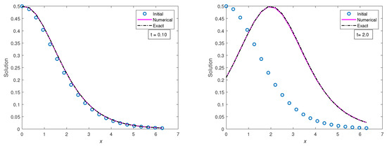
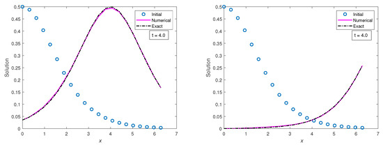
Figure 21. Plots of initial, numerical and exact solutions vs. x ∈ [0, 2π] at times t = 0.10, 2.0, 4.0, 8.0, using the classical finite difference scheme with Δt = ${10}^{-2}$ and Δx = $\frac{\pi }{10}$.

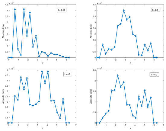
Figure 22. Plots of absolute errors vs. x at times $t=0.10,2.0,4.0,8.0$, using a classical finite difference scheme with $\Delta t={10}^{-2}$ and $\Delta x={\displaystyle \frac{\pi }{10}}$.

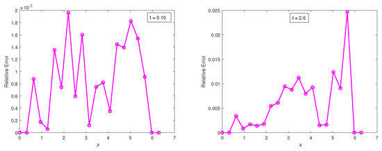
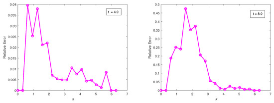
Figure 23. Plots of relative errors vs. x at times $t=0.10,2.0,4.0,8.0$, using the classical finite difference scheme with $\Delta t={10}^{-2}$ and $\Delta x={\displaystyle \frac{\pi }{10}}$.

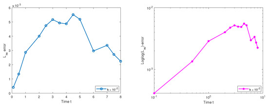
Figure 24. Plot of the maximum error vs. time $t\in [0,8.0]$ and the loglog plot of the maximum error vs. time t with $\Delta x=\frac{\pi }{10}$ and $\Delta t=1.0\times {10}^{-2}$, using the standard finite difference scheme, respectively.

9. Conclusions

In this paper, the performance of the VHPM and classical finite difference methods were compared when solving the linear, as well as the non-linear, KdV equation in 1D- and 2D-space for five different cases:

(i)

case 1: 1D linear homogeneous,

(ii)

case 2: 1D linear non-homogeneous,

(iii)

case 3: 2D linear homogeneous,

(iv)

case 4: 2D linear non-homogeneous.

(v)

case 5: 1D non-linear homogeneous.

We obtained the stability region of the classical finite difference schemes for the five different equations considered. The schemes were tested for the five different cases for short, medium and long time propagation.

For case 1, VHPM produced excellent results for short propagation time and it performed well for medium propagation time; however, it performed poorly for long time propagation. The standard finite difference schemes performed well for short, medium and long time propagation.

VHPM faces some dificulties for case 2 for which the source terms consist of sine and cosine terms; the scheme is quite dissipative even for short propagation time. In contrast, the classical finite difference scheme resolved case 2 quite efficiently for short, medium and long time propagation.

For case 3, the classical finite difference scheme performed well for short, medium and long time propagation, with a relative error of order ${10}^{-4}$ to ${10}^{-2}.$ VHPM performed excellently for short and medium time propagation, but its accuracy deteriorated for longer time propagation, for example, at time 2.0, with a relative error of order ${10}^{-1}$ to ${10}^{-0}.$

With respect to case 4, the classical finite difference scheme performed well for short, medium and long time propagation with a relative error of order ${10}^{-10}$ to ${10}^{-9}$, as shown in Table 4. Due to the nature of the source term used for this problem, VHPM quickly converged to the exact solution in the first two iterations; there was rapid convergence to the exact solution.

For case 5, the VHPM provided a very good result for short time propagation but performed satisfactorily for medium time propagation. The classical schemes performed well for short, medium and long time propagation, with a relative error of order ${10}^{-3}$ to ${10}^{-1}$.

In sum, we conclude that the VHPM was able to efficiently solve numerical Experiments 1, 3, 5 for short and medium time propagation. The VHPM was not effective in solving Experiment 2, but was effective in solving Experiment 4 for different times of propagation. We can also deduce that the classical finite difference scheme was quite efficient in solving all the five experiments for short, medium and long time propagation.

This study provides a basis for constructing numerical methods for more complicated PDEs, such as time and space fractional KdV, KdV-Burgers and stochastic KdV equations, which model real world phenomena, such as wave dynamics [43], geophysical flows, tsunami models, tectonic dynamics [12] and cosmic inflations [11].

References

- Palencia, J.L.D. Travelling waves and instability in a Fisher-KPP problem with a nonlinear advection and a high-order diffusion. Eur. Phys. J. 2021, 136, 774. [Google Scholar] [CrossRef]
- Palencia, J.L.D. Travelling waves approach in a parabolic coupled system for modelling the behaviour of substances in a fuel tank. Appl. Sci. 2021, 11, 5846. [Google Scholar] [CrossRef]
- Palencia, J.L.D.; Ur Rahman, S.; Naranjo, A. Analysis of travelling wave solutions for Eyring-Powell fluid formulated with a degenerate diffusivity and a Darcy-Forchheimer law. AIMS Math. 2022, 7, 6898–6914. [Google Scholar] [CrossRef]
- Ablowitz, M.J.; Clarkson, P.A. Solitons, Nonlinear Evolution Equations and Inverse Scattering; Cambridge University Press: Cambridge, UK, 1999; Volume 149. [Google Scholar]
- Constantin, A.; Escher, J. Wave breaking for nonlinear nonlocal shallow water equations. Acta Math. 1998, 181, 229–243. [Google Scholar] [CrossRef]
- Korteweg, D.J.; de Vries, G. On the change of form of long waves advancing in a rectangular canal, and on a new type of long stationary waves. Philos. Mag. 1895, 39, 422–443. [Google Scholar] [CrossRef]
- Kenig, C.E.; Ponce, G.; Vega, L. A bilinear estimate with applications to the KdV equation. J. Am. Math. Soc. 1996, 9, 573–603. [Google Scholar] [CrossRef]
- Bhrawy, A.H.; Doha, E.H.; Ezz-Eldien, S.S. A numerical technique based on the shifted Legendre polynomials for solving the time-fractional coupled KdV equations. Calcolo 2016, 53, 1–17. [Google Scholar] [CrossRef]
- Zabusky, N.J.; Kruskal, M.D. Interaction of “solitons” in a collisionless plasma and the recurrence of initial states. Phys. Rev. Lett. 1965, 15, 240. [Google Scholar] [CrossRef]
- Guo, M.; Fu, C.; Zhang, Y. Study of ion-acoustic solitary waves in a magnetized plasma using the three-dimensional time-space fractional schamel-KdV equation. Complexity 2018, 2018, 6852548. [Google Scholar] [CrossRef]
- Lidsey, J.E. Cosmology and the Korteweg-de Vries equation. Phys. Rev. D 2012, 86, 123523. [Google Scholar] [CrossRef]
- Lakshmanan, M. Solitons, Tsunamis and Oceanographical Applications of. In Encylopedia of Complexity and Dynamical Systems; Meyers, R., Ed.; Springer: New York, NY, USA, 2009; pp. 8506–8521. [Google Scholar] [CrossRef]
- Pelloni, B.; Dougalis, V.A. Numerical solution of some nonlocal, nonlinear dispersive wave equations. J. Nonlinear Sci. 2000, 10, 1–22. [Google Scholar] [CrossRef]
- Sewell, G. Analysis of a Finite Element Method; Springer Science & Business Media: Berlin/Heidelberg, Germany, 2012. [Google Scholar]
- Huntul, M.J.; Tamsir, M.; Ahmadini, A.A.H.; Thottoli, S.R. A novel collocation technique for parabolic partial differential equations. Ain Shams Eng. J. 2022, 13, 101497. [Google Scholar] [CrossRef]
- Gelu, F.W.; Duressa, G.F. A uniformly convergent collocation method for singularly perturbed delay parabolic reaction-diffusion problem. Abstr. Appl. Anal. 2021, 2021, 11. [Google Scholar] [CrossRef]
- Luo, W.H.; Huang, T.Z.; Gu, X.M.; Liu, Y. Barycentric rational collocation methods for a class of nonlinear parabolic partial differential equations. Appl. Math. Lett. 2017, 68, 13–19. [Google Scholar] [CrossRef]
- Samuel, F.M.; Motsa, S.S. A highly accurate trivariate spectral collocation method of solution for two-dimensional nonlinear initial-boundary value problems. Appl. Math. Comput. 2019, 360, 221–235. [Google Scholar] [CrossRef]
- Adomian, G. Solving Frontier Problems of Physics: The Decomposition Method; Kluwer Academic Publishers: Amsterdam, The Netherlands, 1994. [Google Scholar]
- Adomian, G. A review of decomposition method and some recent results for nonlinear equation. Math. Comput. Model. 1992, 13, 17–43. [Google Scholar] [CrossRef]
- Abassy, T.A.; El-Tawil, M.A.; Saleh, H.K. The solution of KdV and mKdV equations using Adomian Padé approximation. Int. J. Nonl. Sci. Num. Simul. 2004, 5, 327–339. [Google Scholar] [CrossRef]
- He, J.H. Variational iteration method—A kind of non-linear analytical technique: Some examples. Int. J. Non-Linear Mech. 1999, 34, 699–708. [Google Scholar] [CrossRef]
- Wazwaz, A.M. A study on linear and nonlinear Schrödinger equations by the variational iteration method. Chaos Solit. 2008, 37, 1136–1142. [Google Scholar] [CrossRef]
- He, J.H. Homotopy perturbation technique. Comput. Methods Appl. Mech. Eng. 1999, 178, 257–262. [Google Scholar] [CrossRef]
- He, J.H. Homotopy perturbation method: A new non-linear analytical technique. Appl. Math. Comput. 2003, 135, 73–79. [Google Scholar] [CrossRef]
- Inokuti, M.; Sekine, H.; Mura, T. General use of the Lagrange multiplier in nonlinear mathematical physics. In Variational Method in the Mechanics of Solids; Nemat-Naseer, S., Ed.; Pergamon Press: New York, NY, USA, 1978; pp. 156–162. [Google Scholar]
- Wazwaz, A.M. A comparison between the variational iteration method and Adomian decomposition method. J. Comput. Appl. Math. 2007, 207, 129–136. [Google Scholar] [CrossRef]
- Dehghan, Z.M.; Shakeri, F. Use of He’s Homotopy perturbation method for solving a partial differential equation arising in modeling of flow in porous media. J. Porous Media 2008, 11, 765–778. [Google Scholar] [CrossRef]
- Karunakar, P.; Chakraverty, S. Differential quadrature method for solving fifth-order KdV equations. In Recent Trends in Wave Mechanics and Vibrations; Springer: Singapore, 2020; pp. 361–369. [Google Scholar] [CrossRef]
- Ahmad, H.; Khan, T.A.; Stanimirovic, P.S.; Ahmad, I. Modified variational iteration technique for the numerical solution of fifth order KdV-type equations. J. Appl. Comput. Mech. 2020, 6, 1220–1227. [Google Scholar] [CrossRef]
- Zahra, W.K.; Ouf, W.A.; El-Azab, M.S. B-spline soliton solution of the fifth order KdV type equations. AIP Conf. Proc. 2013, 1558, 568–572. [Google Scholar] [CrossRef]
- Wazwaz, A.M. The variational iteration method for rational solutions for KdV, K(2,2), Burgers, and cubic Boussinesq equations. J. Comput. Appl. Math. 2007, 207, 18–23. [Google Scholar] [CrossRef]
- Park, C.; Nuruddeen, R.I.; Ali, K.K.; Muhammad, L.; Osman, M.S.; Baleanu, D. Novel hyperbolic and exponential ansatz methods to the fractional fifth-order Korteweg–de Vries equations. Adv. Differ. Equ. 2020, 1, 627. [Google Scholar] [CrossRef]
- Aderogba, A.A.; Appadu, A.R. Classical and Multisymplectic Schemes for Linearized KdV Equation: Numerical Results and Dispersion Analysis. Fluids 2021, 6, 214. [Google Scholar] [CrossRef]
- Appadu, A.R.; Kelil, A.S. On Semi-Analytical Solutions for Linearized Dispersive KdV equation. Mathematics 2020, 8, 1769. [Google Scholar] [CrossRef]
- Appadu, A.R.; Kelil, A.S. Comparison of modified ADM and classical finite difference method for some third-order and fifth-order KdV equations. Demonstr. Math. 2021, 54, 377–409. [Google Scholar] [CrossRef]
- Kelil, A.S.; Appadu, A.R. Shehu-Adomian decomposition method for dispersive KdV-type equations. In Mathematical Analysis and Applications; Springer: Singapore, 2021; pp. 103–129. [Google Scholar] [CrossRef]
- Appadu, A.R.; Kelil, A.S. Solution of 3D linearized KdV equation using reduced differential transform method. AIP Conf. Proc. 2022, 2425, 020016. [Google Scholar] [CrossRef]
- Matinfar, M.; Mahdavi, M.; Raeisi, Z. The variational homotopy perturbation method for analytic treatment for linear and nonlinear ordinary differential equations. J. Appl. Math. Inform. 2010, 28, 845–862. [Google Scholar]
- He, J.H.; Wu, X.H. Construction of solitary solution and compacton-like solution by variational iteration method. Chaos Solit. 2006, 29, 108–113. [Google Scholar] [CrossRef]
- Matinfar, M.; Mahdavi, M.; Raeisy, Z. The implementation of variational homotopy perturbation method for Fisher’s equation. Int. J. Nonlinear Sci. 2010, 9, 188–194. [Google Scholar]
- Fernández, F.M. On the variational homotopy perturbation method for nonlinear oscillators. J. Math. Phys. 2012, 53, 024101. [Google Scholar] [CrossRef]
- Wazwaz, A.M. Partial Differential Equations and Solitary Waves Theory; Higher Education: Beijing, China; Springer: Berlin/Heidelberg, Germany, 2009. [Google Scholar]
- Wazwaz, A.M. An analytic study on the third-order dispersive partial differential equations. Appl. Math. Comput. 2003, 142, 511–520. [Google Scholar] [CrossRef]
- Wazwaz, A.M. Necessary conditions for the appearance of noise terms in decomposition solution series. J. Math. Anal. Appl. 1997, 5, 265–274. [Google Scholar] [CrossRef]
- Wazwaz, A.M. Partial Differential Equations: Methods and Applications; Balkema Publishers: Lisse, The Netherlands, 2002. [Google Scholar]
- Goswami, V.; Singh, J.; Kumar, D. Numerical simulation of fifth order KdV equation occurring in magneto-acoustic waves. AIN Shams Eng. J. 2018, 9, 2265–2273. [Google Scholar] [CrossRef]
- Mohyud-Din, S.T.; Yildirim, A.; Sezer, S.A.; Usman, M. Modified variational iteration method for free-convective boundary-layer equation using Padé approximation. Math. Prob. Eng. 2010, 2010, 318298. [Google Scholar] [CrossRef]
- Adomian, G.; Rach, R. Noise terms in decomposition solution series. Comp. Math. Appl. 1992, 24, 61–64. [Google Scholar] [CrossRef]
- Taha, T.R.; Ablowitz, M.I. Analytical and numerical aspects of certain nonlinear evolution equations III, Numerical, Korteweg-de Vries equation. J. Comput. Phys. 1984, 55, 231–253. [Google Scholar] [CrossRef]
- Appadu, A.R.; Chapwanya, M.; Jejeniwa, O.A. Some optimised schemes for 1D Korteweg-de-Vries equation. Prog. Comput. Fluid Dyn. 2017, 17, 250–266. [Google Scholar] [CrossRef]
Publisher’s Note: MDPI stays neutral with regard to jurisdictional claims in published maps and institutional affiliations. |
© 2022 by the authors. Licensee MDPI, Basel, Switzerland. This article is an open access article distributed under the terms and conditions of the Creative Commons Attribution (CC BY) license (https://creativecommons.org/licenses/by/4.0/).