Accelerated Randomized Coordinate Descent for Solving Linear Systems

Abstract

The randomized coordinate descent (RCD) method is a simple but powerful approach to solving inconsistent linear systems. In order to accelerate this approach, the Nesterov accelerated randomized coordinate descent method (NARCD) is proposed. The randomized coordinate descent with the momentum method (RCDm) is proposed by Nicolas Loizou, we will provide a new convergence boundary. The global convergence rates of the two methods are established in our paper. In addition, we show that the RCDm method has an accelerated convergence rate by choosing a proper momentum parameter. Finally, in numerical experiments, both the RCDm and the NARCD are faster than the RCD for uniformly distributed data. Moreover, the NARCD has a better acceleration effect than the RCDm and the Nesterov accelerated stochastic gradient descent method. When the linear correlation of matrix A is stronger, the NARCD acceleration is better.

1. Introduction

Consider a large-scale overdetermined linear system

$$Ax=b,$$

(1)

where $A\in R^{m\times n}$, $m\ge n$. We can solve the least-squares problem $mi{n}_x{\parallel b-Ax\parallel }^2$. We assume that the columns of A are normalized:

$$\parallel A_i\parallel =1.$$

(2)

This assumption has no substantial impact on the implementation costs. We could just normalize each $A_i$ the first time the algorithm encounters it. However, we do not assume (2) about the algorithms, and include factors $A_i$ as needed. Regardless of whether normalization is performed, our randomized algorithms yield the same sequence of iterates.

The coordinate descent (CD) technique [1], which can also be produced by applying the conventional Gauss−Seidel iteration method to the following normal equation [2], is one of the iteration methods that may be used to solve the problem (1) cheaply and effectively.

$$A^{T}Ax=A^{T}b,$$

and it is also the same as the quadratic programming problem with no constraints.

$$minf\left(x\right)=\frac{1}{2}{x}^T{A}^{T}Ax-b^{T}Ax,x\in R^n.$$

From [1], we can obtain

$$x^{k+1}=x^k+\frac{⟨A_i,b-Ax⟩}{\parallel A_i{\parallel }^2}{e}_i.$$

(3)

In solving problem (1), the coordinate descent approach has a long history of addressing optimization issues and various applications in a wide range of fields such as biological feature selection [3], machine learning [4], protein structure [5], tomography [6,7], and so on. Inspired by the randomized coordinate descent (RCD) method, a lot of related works were presented, such as greedy versions of the randomized coordinate descent [8,9] and block versions of the randomized coordinate descent [10,11,12]. The coordinate descent method is a column projection method and the Kaczmarz [13] method is a row projection method. The RCD method is inspired by the randomized Kaczmarz(RK) [14] method. For the Kaczmarz-type approach; a lot of relevant work has also been conducted. Readers can refer to [15,16,17,18,19,20].

In this paper, for solving large systems of linear equations, we use two methods to accelerate the RCD method. First, we obtained an accelerated RCD method by adding Nesterov’s acceleration mechanism to the traditional RCD algorithm, called the Nesterov accelerated randomized coordinate descent method (NARCD). It is commonly known that by using an appropriate multi-step technique [21], the traditional gradient method may be turned into a quicker system. To solve the number of unconstrained minimization problems with strongly convex objectives, Nesterov improved this accelerated format [22]. Second, we can apply the heavy ball method (momentum method) to accelerate the RCD. Polyak invented the heavy ball method [23], which is a common approach for speeding up the convergence rate of gradient-type algorithms. Many researchers looked into variations of the heavy ball method, see [24]. By these two methods—to accelerate the RCD—the Nesterov accelerated randomized coordinate descent method (NARCD) and the randomized coordinate descent with momentum method (RCDm) were obtained.

In this paper, given a positive semidefinite matrix M, ${\parallel x\parallel }_M$ is defined as $\sqrt{x^{T}Mx}$, $⟨.⟩$ and $\parallel .\parallel$ stands for the scalar product and the spectral norm, where the column vector is denoted by $e_i$, with 1 at the ith position and 0 elsewhere. In addition, for a given matrix A, $A_i$, ${\parallel A\parallel }_F$, ${\sigma }_{min}\left(A\right)$, and $A^T$ are used to denote its ith column, Frobenius norm, the smallest nonzero singular value, and the transpose of A respectively. $A^{+}$ is the Moore–Penrose pseudoinverse of A. Note that ${\lambda }_1=\frac{1}{\parallel {\left(A{A}^T\right)}^{+}\parallel }$. Let us denote $i\left(k\right)$ as the index randomly generated at iteration k, and let $I\left(k\right)$ denote all random indices that occurred or before iteration k, so that

$$I\left(k\right)=\left\{i\right(k),i(k-1),...,i(0\left)\right\},$$

the sequences $x_{k+1}$,$y_{k+1}$,$v_{k+1}$ are determined by $I\left(k\right)$. In the following part of the proof, we use $E_{i\left(k\right)\left|I\right(k-1)}(.)$ to denote the expectation of a random variable condition of $I(k-1)$ with respect to the index $i\left(k\right)$. So that

$$E_{I\left(k\right)}(.)=E_{I(k-1)}\left(E_{i\left(k\right)\left|I\right(k-1)}(.)\right).$$

(4)

The organization of this paper is as follows. In Section 2, we propose the NARCD method naturally and prove the convergence of the method. In Section 3, we propose the RCDm method and prove its convergence. In Section 4, to demonstrate the efficacy of our new methods, several numerical examples are offered. Finally, we present some brief concluding remarks in Section 5.

2. Nesterov’s Accelerated Randomized Coordinate Descent

The NARCD algorithm applies the Nesterov accelerated procedure [22], which is more well-known in terms of the gradient descent algorithm. Moreover, the Nesterov acceleration scheme creates the sequences $\left\{x_k\right\}$, $\left\{y_k\right\}$, and $\left\{v_k\right\}$. When applied to $mi{n}_{x}f\left(x\right)$, gradient descent sets $x_{k+1}=x_k-{\theta }_k\nabla f\left(x\right)$, where $\nabla f$ is the objective gradient and ${\theta }_k$ is the step-size. We define the following iterative scheme:

$$\begin{array}{cc}\hfill & y_k={\alpha }_k{v}_k+(1-{\alpha }_k)x_k,\hfill \\ & x_{k+1}=y_k-{\theta }_k\nabla f\left(y_k\right),\hfill \\ & v_{k+1}={\beta }_k{v}_k+(1-{\beta }_k)y_k-{\gamma }_k\nabla f\left(y_k\right).\hfill \end{array}$$

The aforementioned scheme’s key addition is that it employs acceptable values for the parameters ${\alpha }_k$, ${\beta }_k$, and ${\gamma }_k$, resulting in improved convergence in traditional gradient descent. In [25], the Nesterov-accelerated procedure is applied to the Kaczmarz method, which is a row action method. The RCD is a column action method and the Nesterov-accelerated procedure can be applied in the same way. The relationship between parameters ${\alpha }_k$, ${\beta }_k$, and ${\gamma }_k$ is given in [22,25]. Now, using the general setup of Nesterov’s scheme, we can obtain the NARCD algorithm (Algorithm 1).

The framework of the NARCD method is given as follows.

Algorithm 1 Nesterov’s accelerated randomized coordinate descent method (NARCD)

Input:$A\in R^{m\times n}$, $b\in R^m$, $K\in R$, $x^{\left(0\right)}\in R^n$, $\lambda \in \left[0,{\lambda }_1\right]$. 1: Initialize $v_0=x_0$, ${\gamma }_{-1}=0$, $k=0$. 2: while$k<K$do 3:    Choose ${\gamma }_k$ to be the larger root of $${\gamma }_k^2-\frac{{\gamma }_k}{n}=(1-\frac{{\gamma }_k\lambda }{n}){\gamma }_{k-1}^2$$ (5) 4:    Set ${\alpha }_k$ and ${\beta }_k$ as follows: $${\alpha }_k=\frac{n-{\gamma }_k\lambda }{{\gamma }_k(n^2-\lambda )}$$ (6) $${\beta }_k=1-\frac{\lambda {\gamma }_k}{n}$$ (7) 5:    Set $y_k={\alpha }_k{v}_k+(1-{\alpha }_k)x_k$ 6:    Choose $i=i\left(k\right)$ from $\left\{1,2,...,n\right\}$ with equal probability 7:    $x_{k+1}=y_k+\frac{⟨A_i,b-A{y}_k⟩}{{∥A_i∥}^2}{e}_i$ 8:    Set $v_{k+1}={\beta }_k{v}_k+(1-{\beta }_k)y_k+{\gamma }_k\frac{⟨A_i,b-A{y}_k⟩}{{∥A_i∥}^2}{e}_i$ 9:    $k=k+1$ 10: end while Output:$x_K$

Remark 1.

In order to avoid the calculation of the product of matrix and vector ($A{y}_k$ in steps 7 and 8), we adopt the following

$$\begin{array}{cc}\hfill & Y_k={\alpha }_k{V}_k+(1-{\alpha }_k)X_k,\hfill \\ & Z_k=b-Y_k,\hfill \\ & {\mu }_k=\frac{⟨A_i,Z_k⟩}{{∥A_i∥}^2},\hfill \\ & X_{k+1}=Y_k+{\mu }_k{A}_i,\hfill \\ & V_{k+1}={\beta }_k{V}_k+(1-{\beta }_k)Y_k+\left({\gamma }_k{\mu }_k\right)A_i,\hfill \end{array}$$

and $X_0=A{x}_0$, $V_0=X_0$. At the same time, we can use $r_k=b-Y_k$ to estimate the residue.

Lemma 1.

For any solution $x^{\ast }$ to $A^{T}A{x}^{\ast }=A^{T}b$, $y\in R^n$ and $P\left(y\right)=y+\frac{⟨A_i,b-Ay⟩}{{∥A_i∥}^2}{e}_i$, ${∥A_i∥}^2=1$. We can obtain

$$E_i({\parallel A(P\left(y\right)-x^{\ast })\parallel }^2)={\parallel A(y-x^{\ast })\parallel }^2-\frac{1}{n}{\parallel A^T(Ay-b)\parallel }^2.$$

(8)

where a random variable i satisfies the uniform distribution of the set {1,2,..,n}.

Proof. 

Using $E_i$ to donate the expectation with respect to the index i, we have

$$\begin{array}{cc}\hfill & E_i({\parallel A(P\left(y\right)-x^{\ast })\parallel }^2)\hfill \\ & =E_i({\parallel A(y+⟨A_i,b-Ay⟩e_i-x^{\ast })\parallel }^2)\hfill \\ & =E_i(\parallel (A(y-x^{\ast })+⟨A_i,b-Ay⟩A_i){\parallel }^2)\hfill \\ & =\parallel A(y-x^{\ast }){\parallel }^2+E_i(\parallel ⟨A_i,b-Ay⟩A_i{\parallel }^2)+2E_i⟨A(y-x^{\ast }),⟨A_i,b-Ay⟩A_i⟩\hfill \\ & =\parallel A(y-x^{\ast }){\parallel }^2+\frac{1}{n}{\parallel A^{T}A(y-x^{\ast })\parallel }^2+\frac{2}{n}⟨A(y-x^{\ast }),A{A}^T(b-Ay)⟩\hfill \\ & =\parallel A(y-x^{\ast }){\parallel }^2-\frac{1}{n}{\parallel A^{T}A(y-x^{\ast })\parallel }^2,\hfill \end{array}$$

where the last equality uses $A^{T}A{x}^{\ast }=A^{T}b$.    □

Lemma 2.

For any $y\in R^n$, we have

$$E_i\left(\parallel A_i⟨A_i,b-Ay⟩{\parallel }_{{\left(A{A}^T\right)}^{+}}^2\right)\le \frac{1}{n}{\parallel A^{T}A(y-x^{\ast })\parallel }^2,$$

(9)

where the random variable i satisfies the uniform distribution of the set {1,2,..,n}.

Proof. 

We know the compact singular value decomposition of A as $A=U\Sigma V^T$, where $U\in R^{m\times r}, V\in R^{n\times r}, \Sigma \in R^{r\times r}$, r is the rank of A, and $U^{T}U=I, V^{T}V=I,$ Σ is the positive diagonal, and we can obtain ${\left(A{A}^T\right)}^{+}=U{\Sigma }^{-2}{U}^T$.

$$\begin{array}{cc}\hfill & E_i\left(\parallel A_i⟨A_i,b-Ay⟩{\parallel }_{{\left(A{A}^T\right)}^{+}}^2\right)\hfill \\ & =\frac{1}{n}\sum _{i=1}^n⟨A_i⟨A_i,b-Ay⟩,{\left(A{A}^T\right)}^{+}{A}_i⟨A_i,b-Ay⟩⟩\hfill \\ & =\frac{1}{n}trace[{\left(A{A}^T\right)}^{+}\sum _{i=1}^n{A}_i{⟨A_i,b-Ay⟩}^2{A}_i^T]\hfill \\ & =\frac{1}{n}trace[{\left(A{A}^T\right)}^{+}Adiag{\left(A^T(b-Ay)\right)}^2{A}^T]\hfill \\ & =\frac{1}{n}trace[U{\Sigma }^{-2}{U}^{T}U\Sigma V^{T}diag{\left(A^T(b-Ay)\right)}^{2}V\Sigma U^T]\hfill \\ & =\frac{1}{n}trace[U{\Sigma }^{-1}{V}^{T}diag{\left(A^T(b-Ay)\right)}^{2}V\Sigma U^T]\hfill \\ & =\frac{1}{n}trace[V^{T}diag{\left(A^T(b-Ay)\right)}^{2}V]\hfill \\ & =\frac{1}{n}{\parallel diag\left(A^T(b-Ay)\right)V\parallel }_F^2\hfill \\ & =\frac{1}{n}\sum _{i=1}^n{\left(⟨A_i,b-Ay⟩\right)}^2{\parallel v_i\parallel }^2\hfill \\ & \le \frac{1}{n}{\parallel A^{T}A(y-x^{\ast })\parallel }^2.\hfill \end{array}$$

As the sixth equation is a consequence of trace(ABC)=trace(BCA), and $V={[v_1,v_2,...,v_n]}^T$, $\parallel v_i{\parallel }^2\le 1$, so that the last inequality holds.    □

Lemma 3.

As all $n^2-\lambda >0$, the following definition:

$${\alpha }_k=\frac{n-{\gamma }_k\lambda }{{\gamma }_k(n^2-\lambda )},{\beta }_k=1-\frac{\lambda {\gamma }_k}{n}$$

for both sequences $\left\{{\alpha }_k\right\}$, $\left\{{\beta }_k\right\}$ lie in the interval $[0,1]$ if and only if ${\gamma }_k$ satisfies the following property:

$$\frac{1}{n}\le {\gamma }_k\le \frac{n}{\lambda },$$

and ${\gamma }_{-1}=0$, if ${\gamma }_{k-1}\le \frac{1}{\sqrt{\lambda }}$, then ${\gamma }_k\in [{\gamma }_{k-1},\frac{1}{\sqrt{\lambda }}]$.

Proof. 

The first part of the lemma clearly holds. For the second part, recall from (5) that ${\gamma }_k$ is the larger root of the following convex quadratic function:

$$g\left(\gamma \right)={\gamma }^2-\frac{\gamma }{n}(1-\lambda {\gamma }_{k-1}^2)-{\gamma }_{k-1}^2,$$

we note the following:

$$g\left({\gamma }_{k-1}\right)=-({\gamma }_{k-1}/n)(1-\lambda {\gamma }_{k-1}^2)\le 0,$$

$$\begin{array}{cc}\hfill g(\frac{1}{\sqrt{\lambda }})& =\frac{1}{\lambda }-\frac{1}{n\sqrt{\lambda }}(1-\lambda {\gamma }_{k-1}^2)-{\gamma }_{k-1}^2\hfill \\ & =\frac{1}{\lambda }-\frac{1}{n\sqrt{\lambda }}+{\gamma }_{k-1}^2(\frac{\sqrt{\lambda }}{m}-1)\hfill \\ & \ge \frac{1}{\lambda }-\frac{1}{n\sqrt{\lambda }}+\frac{1}{\lambda }(\frac{\sqrt{\lambda }}{m}-1)=0,\hfill \end{array}$$

which together imply that ${\gamma }_k\in [{\gamma }_{k-1},\frac{1}{\sqrt{\lambda }}]$.    □

Lemma 4.

Let a, b, and c be any vector in $R^n$, then the following identity holds:

$$2⟨a-c,c-b⟩={\parallel a-b\parallel }^2{-\parallel a-c\parallel }^2-{\parallel c-b\parallel }^2.$$

(10)

Theorem 1.

The coordinate descent method with Nesterov’s acceleration for solving linear equations, $\lambda \in [0,{\lambda }_1]$ and $x^{\ast }$ is the least-squares solution. Define ${\sigma }_1=1+\frac{\sqrt{\lambda }}{2n}$ and ${\sigma }_2=1-\frac{\sqrt{\lambda }}{2n}$, then for all $k\ge 0$, we have the following

$$E(\parallel A(x_{k+1}-x^{\ast }){\parallel }^2)\le \frac{4\lambda \parallel A(x_0-x^{\ast }){\parallel }^2}{{({\sigma }_1^{k+1}-{\sigma }_2^{k+1})}^2}$$

(11)

and

$$E(\parallel A(v_{k+1}-x^{\ast }){\parallel }_{{\left(A{A}^T\right)}^{+}}^2)\le \frac{4\parallel A(x_0-x^{\ast }){\parallel }_{{\left(A{A}^T\right)}^{+}}^2}{{({\sigma }_1^{k+1}+{\sigma }_2^{k+1})}^2}.$$

(12)

Proof. 

We follow the standard notation and steps shown in [22,25]; by (5) and (6), the following relation holds:

$$\frac{1-{\alpha }_k}{{\alpha }_k}=\frac{n{\gamma }_{k-1}^2}{{\gamma }_k}.$$

(13)

From (5) and (7), we have

$${\gamma }_k^2-\frac{{\gamma }_k}{n}-{\beta }_k{\gamma }_{k-1}^2=0.$$

(14)

Now, let us define $r_k^2={\parallel A(v_k-x^{\ast })\parallel }_{{\left(A{A}^T\right)}^{+}}^2$. Then we have

$$\begin{array}{cc}\hfill r_{k+1}^2& =\parallel A(v_{k+1}-x^{\ast }){\parallel }_{{\left(A{A}^T\right)}^{+}}^2\hfill \\ & =\parallel A({\beta }_k{v}_k+(1-{\beta }_k)y_k+{\gamma }_k⟨A_i,b-A{y}_k⟩e_i-x^{\ast }){\parallel }_{{\left(A{A}^T\right)}^{+}}^2\hfill \\ & =\parallel A({\beta }_k{v}_k+(1-{\beta }_k)y_k-x^{\ast }){\parallel }_{{\left(A{A}^T\right)}^{+}}^2+{\gamma }_k^2{\parallel A_i⟨A_i,b-A{y}_k⟩\parallel }_{{\left(A{A}^T\right)}^{+}}^2\hfill \\ & +2{\gamma }_k⟨A({\beta }_k{v}_k+(1-{\beta }_k)y_k-x^{\ast }),{\left(A{A}^T\right)}^{+}{A}_i⟨A_i,b-A{y}_k⟩⟩\hfill \\ & =\parallel A({\beta }_k{v}_k+(1-{\beta }_k)y_k-x^{\ast }){\parallel }_{{\left(A{A}^T\right)}^{+}}^2+{\gamma }_k^2{\parallel A_i⟨A_i,b-A{y}_k⟩\parallel }_{{\left(A{A}^T\right)}^{+}}^2\hfill \\ & +2{\gamma }_k⟨A({\beta }_k(\frac{1}{{\alpha }_k}{y}_k-\frac{1-{\alpha }_k}{{\alpha }_k}{x}_k)+(1-{\beta }_k)y_k-x^{\ast }),{\left(A{A}^T\right)}^{+}{A}_i⟨A_i,b-A{y}_k⟩⟩\hfill \\ & =\parallel A({\beta }_k{v}_k+(1-{\beta }_k)y_k-x^{\ast }){\parallel }_{{\left(A{A}^T\right)}^{+}}^2+{\gamma }_k^2{\parallel A_i⟨A_i,b-A{y}_k⟩\parallel }_{{\left(A{A}^T\right)}^{+}}^2\hfill \\ & +2{\gamma }_k⟨A(y_k-x^{\ast })+\frac{1-{\alpha }_k}{{\alpha }_k}{\beta }_{k}A(y_k-x_k),{\left(A{A}^T\right)}^{+}{A}_i⟨A_i,b-A{y}_k⟩⟩.\hfill \end{array}$$

(15)

Now, we divide (15) into three parts and simplify them separately. From the convexity of ${\parallel .\parallel }_{{\left(A{A}^T\right)}^{+}}^2$ and in Lemma 3, we know ${\beta }_k\in [0,1]$. So the first part of (15) is as follows:

$$\begin{array}{cc}\hfill & \parallel A({\beta }_k{v}_k+(1-{\beta }_k)y_k-x^{\ast }){\parallel }_{{\left(A{A}^T\right)}^{+}}^2\hfill \\ & =\parallel A({\beta }_k(v_k-x^{\ast })+(1-{\beta }_k)(y_k-x^{\ast })){\parallel }_{{\left(A{A}^T\right)}^{+}}^2\hfill \\ & \le {\beta }_k\parallel A(v_k-x^{\ast }){\parallel }_{{\left(A{A}^T\right)}^{+}}^2+(1-{\beta }_k){\parallel A(y_k-x^{\ast })\parallel }_{{\left(A{A}^T\right)}^{+}}^2\hfill \\ & ={\beta }_k\parallel A(v_k-x^{\ast }){\parallel }_{{\left(A{A}^T\right)}^{+}}^2+\frac{{\gamma }_k\lambda }{n}{\parallel A(y_k-x^{\ast })\parallel }_{{\left(A{A}^T\right)}^{+}}^2\hfill \\ & \le {\beta }_k\parallel A(v_k-x^{\ast }){\parallel }_{{\left(A{A}^T\right)}^{+}}^2+\frac{{\gamma }_k}{n}{\parallel A(y_k-x^{\ast })\parallel }^2,\hfill \end{array}$$

(16)

where the last inequality makes use of $\lambda \le {\lambda }_1=\frac{1}{\parallel {\left(A{A}^T\right)}^{+}\parallel }$. Using Lemmas 1 and 2, the second part of (15) is as follows:

$$\begin{array}{cc}\hfill & {\gamma }_k^2{E}_{i\left(k\right)\left|I\right(k-1)}\left(\parallel A_i⟨A_i,b-A{y}_k⟩{\parallel }_{{\left(A{A}^T\right)}^{+}}^2\right)\hfill \\ & \le \frac{{\gamma }_k^2}{n}{\parallel A^{T}A(y_k-x^{\ast })\parallel }^2\hfill \\ & ={\gamma }_k^2{\parallel A(y_k-x^{\ast })\parallel }^2-{\gamma }_k^2{E}_{i\left(k\right)\left|I\right(k-1)}\left({\parallel A(x_{k+1}-x^{\ast })\parallel }^2\right).\hfill \end{array}$$

(17)

We use the identity of (8) in the last part of our proof. We take expectations in the last part of (15) and can obtain

$$\begin{array}{cc}\hfill & 2{\gamma }_k{E}_{i\left(k\right)\left|I\right(k-1)}(⟨A(y_k-x^{\ast })+\frac{1-{\alpha }_k}{{\alpha }_k}{\beta }_{k}A(y_k-x_k),{\left(A{A}^T\right)}^{+}{A}_i⟨A_i,b-A{y}_k⟩⟩)\hfill \\ & =2{\gamma }_k⟨A(y_k-x^{\ast })+\frac{1-{\alpha }_k}{{\alpha }_k}{\beta }_{k}A(y_k-x_k),{\left(A{A}^T\right)}^{+}{E}_{i\left(k\right)\left|I\right(k-1)}{A}_i⟨A_i,b-A{y}_k⟩⟩\hfill \\ & =\frac{2{\gamma }_k}{n}⟨A(y_k-x^{\ast })+\frac{1-{\alpha }_k}{{\alpha }_k}{\beta }_{k}A(y_k-x_k),{\left(A{A}^T\right)}^{+}\sum _{i=1}^n{A}_i⟨A_i,b-A{y}_k⟩⟩\hfill \\ & =\frac{2{\gamma }_k}{n}⟨A(y_k-x^{\ast })+\frac{1-{\alpha }_k}{{\alpha }_k}{\beta }_{k}A(y_k-x_k),{\left(A{A}^T\right)}^{+}A{A}^T(b-A{y}_k)⟩\hfill \\ & =\frac{2{\gamma }_k}{n}⟨A(y_k-x^{\ast })+\frac{1-{\alpha }_k}{{\alpha }_k}{\beta }_{k}A(y_k-x_k),(b-A{y}_k)⟩\hfill \\ & =\frac{2{\gamma }_k}{n}⟨A(y_k-x^{\ast }),b-A{y}_k⟩+\frac{2{\gamma }_k}{n}\frac{1-{\alpha }_k}{{\alpha }_k}{\beta }_k⟨A(y_k-x_k),b-A{y}_k⟩\hfill \\ & =-\frac{2{\gamma }_k}{n}\parallel A(y_k-x^{\ast }){\parallel }^2+{\beta }_k{\gamma }_{k-1}^2(\parallel A(x_k-x^{\ast }){\parallel }^2-\parallel A(y_k-x^{\ast }){\parallel }^2-\parallel A(y_k-x_k){\parallel }^2)\hfill \\ & \le -(\frac{2{\gamma }_k}{n}+{\beta }_k{\gamma }_{k-1}^2)\parallel A(y_k-x^{\ast }){\parallel }^2+{\beta }_k{\gamma }_{k-1}^2{\parallel A(x_k-x^{\ast })\parallel }^2,\hfill \end{array}$$

(18)

where the fifth and sixth equalities make use of the (13), and (10), respectively. Substituting all three parts of (16)–(18) into(15), we have

$$\begin{array}{cc}\hfill & E_{i\left(k\right)\left|I\right(k-1)}\left(r_{k+1}^2\right)\hfill \\ & \le {\beta }_k\parallel A(v_k-x^{\ast }){\parallel }_{{\left(A{A}^T\right)}^{+}}^2+\frac{{\gamma }_k}{n}{\parallel A(y_k-x^{\ast })\parallel }^2\hfill \\ & +{\gamma }_k^2{\parallel A(y_k-x^{\ast })\parallel }^2-{\gamma }_k^2{E}_{i\left(k\right)\left|I\right(k-1)}({\parallel A(x_{k+1}-x^{\ast })\parallel }^2)\hfill \\ & -(\frac{2{\gamma }_k}{n}+{\beta }_k{\gamma }_{k-1}^2)\parallel A(y_k-x^{\ast }){\parallel }^2+{\beta }_k{\gamma }_{k-1}^2{\parallel A(x_k-x^{\ast })\parallel }^2\hfill \\ & ={\beta }_k\parallel A(v_k-x^{\ast }){\parallel }_{{\left(A{A}^T\right)}^{+}}^2+({\gamma }_k^2-\frac{{\gamma }_k}{n}-{\beta }_k{\gamma }_{k-1}^2){\parallel A(y_k-x^{\ast })\parallel }^2\hfill \\ & -{\gamma }_k^2{E}_{i\left(k\right)\left|I\right(k-1)}({\parallel A(x_{k+1}-x^{\ast })\parallel }^2)+{\beta }_k{\gamma }_{k-1}^2{\parallel A(x_k-x^{\ast })\parallel }^2\hfill \\ & ={\beta }_k\parallel A(v_k-x^{\ast }){\parallel }_{{\left(A{A}^T\right)}^{+}}^2-{\gamma }_k^2{E}_{i\left(k\right)\left|I\right(k-1)}({\parallel A(x_{k+1}-x^{\ast })\parallel }^2)+{\beta }_k{\gamma }_{k-1}^2{\parallel A(x_k-x^{\ast })\parallel }^2,\hfill \end{array}$$

(19)

where the last equality is the consequence of (14). Let us define two sequences $\left\{A_k\right\}$,$\left\{B_k\right\}$ as follows:

$$B_{k+1}^2=\frac{B_k^2}{{\beta }_k},A_{k+1}^2={\gamma }_k^2{B}_{k+1}^2,$$

(20)

we know the ${\beta }_k\in (0,1]$, and $B_k\ge 0$, $B_0\ne 0$. We have $B_{k+1}\ge B_k$. Because of the ${\gamma }_{-1}=0$, we have $A_0=0$. Moreover, ${\gamma }_k\in [{\gamma }_{k-1},\frac{1}{\sqrt{\lambda }}]$ in Lemma 3, so that we can obtain that the $\left\{A_k\right\}$ is also an increasing sequence. Now, multiplying both sides of (19) by $B_{k+1}^2$ and using the (20), we have

$$\begin{array}{cc}\hfill & B_{k+1}^2{E}_{i\left(k\right)\left|I\right(k-1)}{\parallel A(v_{k+1}-x^{\ast })\parallel }_{{\left(A{A}^T\right)}^{+}}^2+A_{k+1}^2{E}_{i\left(k\right)\left|I\right(k-1)}{\parallel A(x_{k+1}-x^{\ast })\parallel }^2\hfill \\ & \le B_k^2\parallel A(v_k-x^{\ast }){\parallel }_{{\left(A{A}^T\right)}^{+}}^2+A_k^2{\parallel A(x_k-x^{\ast })\parallel }^2,\hfill \end{array}$$

(21)

and then

$$\begin{array}{cc}\hfill & E_{I\left(k\right)}(B_{k+1}^2\parallel A(v_{k+1}-x^{\ast }){\parallel }_{{\left(A{A}^T\right)}^{+}}^2+A_{k+1}^2{\parallel A(x_{k+1}-x^{\ast })\parallel }^2)\hfill \\ & =E_{I(k-1)}(B_{k+1}^2{E}_{i\left(k\right)\left|I\right(k-1)}\parallel A(v_{k+1}-x^{\ast }){\parallel }_{{\left(A{A}^T\right)}^{+}}^2+A_{k+1}^2{E}_{i\left(k\right)\left|I\right(k-1)}{\parallel A(x_{k+1}-x^{\ast })\parallel }^2)\hfill \\ & \le E_{I(k-1)}(B_k^2\parallel A(v_k-x^{\ast }){\parallel }_{{\left(A{A}^T\right)}^{+}}^2+A_k^2\parallel A(x_k-x^{\ast }){\parallel }^2)\hfill \\ & \le E_{I\left(0\right)}(B_1^2\parallel A(v_1-x^{\ast }){\parallel }_{{\left(A{A}^T\right)}^{+}}^2+A_1^2\parallel A(x_1-x^{\ast }){\parallel }^2)\hfill \\ & \le B_0^2\parallel A(v_0-x^{\ast }){\parallel }_{{\left(A{A}^T\right)}^{+}}^2+A_0^2\parallel A(x_1-x^{\ast }){\parallel }^2)\hfill \\ & =B_0^2{\parallel A(v_0-x^{\ast })\parallel }_{{\left(A{A}^T\right)}^{+}}^2\hfill \\ & =B_0^2{\parallel A(x_0-x^{\ast })\parallel }_{{\left(A{A}^T\right)}^{+}}^2.\hfill \end{array}$$

(22)

So, by the (22), we can obtain

$$\begin{array}{cc}\hfill & E\parallel A(v_{k+1}-x^{\ast }){\parallel }_{{\left(A{A}^T\right)}^{+}}^2\le \frac{B_0^2}{B_{k+1}^2}{\parallel A(x_0-x^{\ast })\parallel }_{{\left(A{A}^T\right)}^{+}}^2,\hfill \\ & E{\parallel A(x_{k+1}-x^{\ast })\parallel }^2\le \frac{B_0^2}{A_{k+1}^2}{\parallel A(x_0-x^{\ast })\parallel }_{{\left(A{A}^T\right)}^{+}}^2,\hfill \end{array}$$

(23)

we now need to analyze the growth of two sequences $\left\{A_k\right\}$ and $\left\{B_k\right\}$. Following the proof in [22,26] for the Nesterov accelerated scheme and the accelerated sampling Kaczmarz Motzkin algorithm [25], we have

$$B_k^2={\beta }_k{B}_{k+1}^2=(1-\frac{\lambda {\gamma }_k}{n})B_{k+1}^2=(1-\frac{\lambda A_{k+1}}{n{B}_{k+1}})B_{k+1}^2.$$

It implies that

$$\begin{array}{cc}\hfill B_k^2& =(1-\frac{\lambda A_{k+1}}{n{B}_{k+1}})B_{k+1}^2\hfill \\ & =B_{k+1}^2-\frac{\lambda }{n}{A}_{k+1}{B}_{k+1},\hfill \end{array}$$

then

$$\frac{\lambda }{n}{A}_{k+1}{B}_{k+1}=B_{k+1}^2-B_k^2=(B_{k+1}-B_k)(B_{k+1}+B_k)\le 2B_{k+1}(B_{k+1}-B_k).$$

Moreover, because the $\left\{B_k\right\}$ and the $\left\{A_k\right\}$ are increasing sequences, we can simplify them and obtain

$$B_{k+1}\ge B_k+\frac{\lambda }{2n}{A}_{k+1}\ge B_k+\frac{\lambda }{2n}{A}_k.$$

(24)

Similarly, we have

$$\begin{array}{cc}\hfill \frac{A_{k+1}^2}{B_{k+1}^2}-\frac{A_{k+1}}{n{B}_{k+1}}& ={\gamma }_k^2-\frac{{\gamma }_k}{n}\hfill \\ & ={\beta }_k{\gamma }_{k-1}^2\hfill \\ & =\frac{A_k^2}{B_{k+1}^2},\hfill \end{array}$$

where the second equality uses (14) and the third equality uses (20). Using the above relationship, we have

$$\begin{array}{cc}\hfill \frac{1}{n}{A}_{k+1}{B}_{k+1}& =A_{k+1}^2-A_k^2\hfill \\ & =(A_{k+1}+A_k)(A_{k+1}-A_k)\hfill \\ & \le 2A_{k+1}(A_{k+1}-A_k).\hfill \end{array}$$

Therefore,

$$A_{k+1}\ge A_k+\frac{B_k}{2n}.$$

(25)

By combining the two expressions of (25) and (24), we have

$$\left[\begin{array}{c}{A}_{k+1}\\ B_{k+1}\end{array}\right]\ge {\left[\begin{array}{cc}1& \frac{1}{2n}\\ \frac{\lambda }{2n}& 1\end{array}\right]}^{k+1}\left[\begin{array}{c}{A}_0\\ B_0\end{array}\right].$$

The Jordan decomposition of the matrix in the above expression is

$$\left[\begin{array}{cc}1& \frac{1}{2n}\\ \frac{\lambda }{2n}& 1\end{array}\right]={\left[\begin{array}{cc}1& 1\\ \sqrt{\lambda }& -\sqrt{\lambda }\end{array}\right]}^{-1}\left[\begin{array}{cc}{\sigma }_1& 0\\ 0& {\sigma }_2\end{array}\right]\left[\begin{array}{cc}1& 1\\ \sqrt{\lambda }& -\sqrt{\lambda }\end{array}\right].$$

Here, ${\sigma }_1=1+\frac{\sqrt{\lambda }}{2n}$ and ${\sigma }_2=1-\frac{\sqrt{\lambda }}{2n}$. Because of $A_0=0$, we have

$$\begin{array}{cc}\hfill \left[\begin{array}{c}{A}_{k+1}\\ B_{k+1}\end{array}\right]& \ge {\left[\begin{array}{cc}1& \frac{1}{2n}\\ \frac{\lambda }{2n}& 1\end{array}\right]}^{k+1}\left[\begin{array}{c}{A}_0\\ B_0\end{array}\right]\hfill \\ & \ge {\left[\begin{array}{cc}1& 1\\ \sqrt{\lambda }& -\sqrt{\lambda }\end{array}\right]}^{-1}{\left[\begin{array}{cc}{\sigma }_1& 0\\ 0& {\sigma }_2\end{array}\right]}^{k+1}\left[\begin{array}{cc}1& 1\\ \sqrt{\lambda }& -\sqrt{\lambda }\end{array}\right]\left[\begin{array}{c}0\\ B_0\end{array}\right]\hfill \\ & =\frac{1}{2}\left[\begin{array}{c}(\frac{{\sigma }_1^{k+1}-{\sigma }_2^{k+1}}{\sqrt{\lambda }})B_0\\ ({\sigma }_1^{k+1}+{\sigma }_2^{k+1})B_0\end{array}\right].\hfill \end{array}$$

The above relationship gives us the growth bound for the sequences $\left\{A_k\right\}$ and $\left\{B_k\right\}$. Substituting these above bounds in (23), we have

$$\begin{array}{cc}\hfill & E\parallel A(v_{k+1}-x^{\ast }){\parallel }_{{\left(A{A}^T\right)}^{+}}^2\le \frac{B_0^2}{B_{k+1}^2}{\parallel A(x_0-x^{\ast })\parallel }_{{\left(A{A}^T\right)}^{+}}^2\le \frac{4\parallel A(x_0-x^{\ast }){\parallel }_{{\left(A{A}^T\right)}^{+}}^2}{{({\sigma }_1^{k+1}+{\sigma }_2^{k+1})}^2},\hfill \\ & E{\parallel A(x_{k+1}-x^{\ast })\parallel }^2\le \frac{B_0^2}{A_{k+1}^2}{\parallel A(x_0-x^{\ast })\parallel }_{{\left(A{A}^T\right)}^{+}}^2\le \frac{4\lambda \parallel A(x_0-x^{\ast }){\parallel }^2}{{({\sigma }_1^{k+1}-{\sigma }_2^{k+1})}^2},\hfill \end{array}$$

and we have completed the proof.     □

Remark 2.

From the relationship between $y_k$, $x_k$, and $v_k$, $y_k={\alpha }_k{v}_k+(1-{\alpha }_k)x_k$, we know that

$$\begin{array}{cc}\hfill & E\parallel A(y_{k+1}-x^{\ast }){\parallel }_{{\left(A{A}^T\right)}^{+}}^2\hfill \\ & =E\parallel A({\alpha }_{k+1}(v_{k+1}-x^{\ast })+(1-{\alpha }_{k+1})(x_{k+1}-x^{\ast })){\parallel }_{{\left(A{A}^T\right)}^{+}}^2\hfill \\ & \le {\alpha }_{k+1}E\parallel A(v_{k+1}-x^{\ast }){\parallel }_{{\left(A{A}^T\right)}^{+}}^2+(1-{\alpha }_{k+1})E{\parallel A(x_{k+1}-x^{\ast })\parallel }_{{\left(A{A}^T\right)}^{+}}^2,\hfill \end{array}$$

and

$$\begin{array}{cc}\hfill \parallel A(x_{k+1}-x^{\ast }){\parallel }_{{\left(A{A}^T\right)}^{+}}^2& \le \parallel A(x_{k+1}-x^{\ast }){\parallel }^2{\parallel {\left(A{A}^T\right)}^{+}\parallel }^2\hfill \\ & =\frac{\parallel A(x_{k+1}-x^{\ast }){\parallel }^2}{{\sigma }_{min}^4\left(A\right)},\hfill \end{array}$$

where the ${\sigma }_{min}^4\left(A\right)$ is the nonzero minimum singular value of A. By the above inequality and Theorem 1, we have

$$\begin{array}{cc}\hfill E\parallel A(y_{k+1}-x^{\ast }){\parallel }_{{\left(A{A}^T\right)}^{+}}^2& \le {\alpha }_{k+1}E\parallel A(v_{k+1}-x^{\ast }){\parallel }_{{\left(A{A}^T\right)}^{+}}^2+\frac{(1-{\alpha }_{k+1})}{{\sigma }_{min}^4\left(A\right)}E{\parallel A(x_{k+1}-x^{\ast })\parallel }^2\hfill \\ & \le (\frac{4{\alpha }_{k+1}}{{({\sigma }_1^{k+1}+{\sigma }_2^{k+1})}^2}+\frac{4(1-{\alpha }_{k+1})\lambda }{{\sigma }_{min}^4\left(AA\right){({\sigma }_1^{k+1}-{\sigma }_2^{k+1})}^2}){\parallel A(x_0-x^{\ast })\parallel }^2.\hfill \end{array}$$

3. Randomized Coordinate Descent with Momentum Method

The iterative formula of the gradient descent (GD) method is as follows,

$$x_{k+1}=x_k-{\lambda }_k\nabla f\left(x_k\right),$$

where ${\lambda }_k$ is a positive step-size parameter. Polyak [23] proposed the gradient descent method with momentum (GDm) by introducing a momentum term $\delta (x_k-x_{k-1})$, which was also known as the heavy ball method

$$x_{k+1}=x_k-{\lambda }_k\nabla f\left(x_k\right)+\delta (x_k-x_{k-1}),$$

where $\delta$ is a momentum parameter. Letting $g\left(x_k\right)$ be an unbiased estimator of the true gradient $\nabla f\left(x_k\right)$, we have the stochastic gradient descent with momentum (mSGD) method.

$$x_{k+1}=x_k-{\lambda }_{k}g\left(x_k\right)+\delta (x_k-x_{k-1}).$$

The randomized coordinate descent with momentum (RCDm) method is proposed in [27]. We will give a new convergence boundary.

The RCDm method takes the explicit iterative form

$$x_{k+1}=x_k+\frac{⟨A_i,b-A{x}_k⟩}{{∥A_i∥}^2}{e}_i+\delta (x_k-x_{k-1}).$$

(26)

The framework of the RCDm method is given as follows (Algorithm 2).

Algorithm 2 Randomized coordinate descent with momentum method (RCDm)

Input:$A\in R^{m\times n}$, $b\in R^m$, $K\in R$, $x^{\left(0\right)}\in R^n$, $\delta$. 1: Initialize $k=0$. 2: while$k<K$do 3:    Choose $i=i\left(k\right)$ from $\left\{1,2,...,n\right\}$ with equal probability 4:    $x_{k+1}=x_k+\frac{⟨A_i,b-A{x}_k⟩}{{∥A_i∥}^2}{e}_i+\delta (x_k-x_{k-1})$ 5:    $k=k+1$ 6: end while Output:$x_K$

Remark 3.

In order to avoid the calculation of the product of matrix and vector ($A{x}_k$ in step 5), we adopt the following method

$$\begin{array}{cc}\hfill & {\alpha }_k=\frac{⟨A_i,r_k⟩}{{∥A_i∥}^2},\hfill \\ & r_{k+1}=(1+\delta )r_k-{\alpha }_k{A}_i-\delta r_{k-1},\hfill \end{array}$$

and $r_0=b-A{x}_0$, $r_{-1}=r_0$.

Lemma 5

([27]). Fix $F_1=F_0\ge 0$ and let ${\left\{F_k\right\}}_{k\ge 0}$ be a sequence of nonnegative real numbers satisfying the relation

$$F_{k+1}\le a_1{F}_k+a_2{F}_{k-1},\forall k\ge 1,$$

where $a_2\ge 0$, $a_1+a_2<1$, and at least one of the coefficients $a_1$, $a_2$ is positive. Then the sequence satisfies the relation $F_{k+1}$$\le q^k(1+\xi )F_0$ for all $k\ge 1$, where $q=\frac{a_1+\sqrt{a_1^2+4a_2}}{2}$ and $\xi =q-a_1\ge 0$. Moreover,

$$q\ge a_1+a_2,$$

with equality if and only if $a_2=0$ (in that case, $q=a_1$ and $\xi =0$).

Theorem 2.

Assume $\delta \ge 0$, and that the expressions $a_1=1-\frac{{\sigma }_{min}^2\left(A\right)}{n}+3\delta -3\frac{\delta {\sigma }_{min}^2\left(A\right)}{n}+2{\delta }^2$ and $a_2=2{\delta }^2+\delta -\frac{\delta {\sigma }_{min}^2\left(A\right)}{n}$ satisfy $a_1+a_2<1$, where ${\sigma }_{min}^2\left(A\right)$ is nonzero minimum singular value of A. Let ${\left\{x_k\right\}}_{k=0}^{\infty }$ be the iteration sequence generated by the RCDm method starting from initial guess $x_0=0$. Then, it holds that

$$E(\parallel A(x_{k+1}-x^{\ast }){\parallel }^2)\le q^k(1+\xi ){\parallel A(x_0-x^{\ast })\parallel }^2,$$

(27)

where $q=\frac{a_1+\sqrt{a_1^2+4a_2}}{2}$, $\xi =q-a_1\ge 0$, $x^{\ast }$ is the least-squares solution. Moreover, $a_1$, $a_2$, q obeys $a_1+a_2\le q<1$.

Proof. 

From the algorithm of RCDm, we have

$$\begin{array}{cc}\hfill & E_{i\left(k\right)\left)\right|I(k-1)}{\parallel A(x_{k+1}-x^{\ast })\parallel }^2\hfill \\ & =E_{i\left(k\right)\left|I\right(k-1)}{\parallel A(x_k+⟨A_i,b-A{x}_k⟩e_i+\delta (x_k-x_{k-1})-x^{\ast })\parallel }^2\hfill \\ & =E_{i\left(k\right)\left|I\right(k-1)}\parallel A(x_k-x^{\ast })+A_i⟨A_i,b-A{x}_k⟩{\parallel }^2+{\delta }^2{\parallel A(x_k-x_{k-1})\parallel }^2\hfill \\ & +2\delta E_{i\left(k\right)\left|I\right(k-1)}⟨A(x_k-x_{k-1}),A(x_k-x^{\ast })+A_i⟨A_i,b-A{x}_k⟩⟩.\hfill \end{array}$$

(28)

We consider the three terms in (28) in turn. For the first term, we have

$$\begin{array}{cc}\hfill & E_{i\left(k\right)\left|I\right(k-1)}{\parallel A(x_k-x^{\ast })+A_i⟨A_i,b-A{x}_k⟩\parallel }^2\hfill \\ & =\parallel A(x_k-x^{\ast }){\parallel }^2+E_{i\left(k\right)\left|I\right(k-1)}{\parallel A_i⟨A_i,b-A{x}_k⟩\parallel }^2\hfill \\ & +2E_{i\left(k\right)\left|I\right(k-1)}⟨A(x_k-x^{\ast }),A_i⟨A_i,b-A{x}_k⟩⟩\hfill \\ & =\parallel A(x_k-x^{\ast }){\parallel }^2+\frac{1}{n}\sum _{i=1}^n{\parallel A_i⟨A_i,b-A{x}_k⟩\parallel }^2\hfill \\ & +\frac{2}{n}\sum _{i=1}^n⟨A(x_k-x^{\ast }),A_i⟨A_i,b-A{x}_k⟩⟩\hfill \\ & =\parallel A(x_k-x^{\ast }){\parallel }^2-\frac{1}{n}{\parallel A^{T}A(x_k-x^{\ast })\parallel }^2\hfill \\ & \le \parallel A(x_k-x^{\ast }){\parallel }^2-\frac{{\sigma }_{min}^2\left(A\right)}{n}{\parallel A(x_k-x^{\ast })\parallel }^2\hfill \\ & =(1-\frac{{\sigma }_{min}^2\left(A\right)}{n}){\parallel A(x_k-x^{\ast })\parallel }^2,\hfill \end{array}$$

(29)

where the last inequality is the consequence of singular value inequality $(\parallel Ax{\parallel }^2\ge {\sigma }_{min}^2\left(A\right)\parallel x{\parallel }^2)$, and $n={\parallel A\parallel }_F^2\ge {\sigma }_{min}^2\left(A\right)$. From the second term, we have

$$\begin{array}{cc}\hfill & {\delta }^2{\parallel A(x_k-x_{k-1})\parallel }^2\hfill \\ & ={\delta }^2{\parallel A(x_k-x^{\ast })-A(x_{k-1}-x^{\ast })\parallel }^2\hfill \\ & \le 2{\delta }^2(\parallel A(x_k-x^{\ast }){\parallel }^2+\parallel A(x_{k-1}-x^{\ast }){\parallel }^2).\hfill \end{array}$$

(30)

From the third term, we have

$$\begin{array}{cc}\hfill & 2\delta E_{i\left(k\right)\left|I\right(k-1)}⟨A(x_k-x_{k-1}),A(x_k-x^{\ast })+A_i⟨A_i,b-A{x}_k⟩⟩\hfill \\ & =2\delta ⟨A(x_k-x_{k-1}),A(x_k-x^{\ast })⟩+2\delta E_{i\left(k\right)\left|I\right(k-1)}⟨A(x_k-x_{k-1}),A_i⟨A_i,b-A{x}_k⟩⟩\hfill \\ & =\delta (\parallel A(x_k-x_{k-1}){\parallel }^2+\parallel A(x_k-x^{\ast }){\parallel }^2-\parallel A(x_{k-1}-x^{\ast }){\parallel }^2)\hfill \\ & +\frac{2\delta }{n}⟨A(x_k-x_{k-1}),\sum _{i=1}^n{A}_i⟨A_i,b-A{x}_k⟩⟩\hfill \\ & =\delta (\parallel A(x_k-x_{k-1}){\parallel }^2+\parallel A(x_k-x^{\ast }){\parallel }^2-\parallel A(x_{k-1}-x^{\ast }){\parallel }^2)\hfill \\ & +\frac{2\delta }{n}⟨A(x_k-x_{k-1}),A{A}^T(b-A{x}_k)⟩\hfill \\ & =\delta (\parallel A(x_k-x_{k-1}){\parallel }^2+\parallel A(x_k-x^{\ast }){\parallel }^2-\parallel A(x_{k-1}-x^{\ast }){\parallel }^2)\hfill \\ & -\frac{2\delta }{n}⟨A^{T}A(x_k-x_{k-1}),A^{T}A(x_k-x^{\ast })⟩\hfill \\ & =\delta (\parallel A(x_k-x_{k-1}){\parallel }^2+\parallel A(x_k-x^{\ast }){\parallel }^2-\parallel A(x_{k-1}-x^{\ast }){\parallel }^2)\hfill \\ & -\frac{\delta }{n}(\parallel A^{T}A(x_k-x_{k-1}){\parallel }^2+\parallel A^{T}A(x_k-x^{\ast }){\parallel }^2-\parallel A^{T}A(x_{k-1}-x^{\ast }){\parallel }^2)\hfill \\ & \le \delta (\parallel A(x_k-x_{k-1}){\parallel }^2+\parallel A(x_k-x^{\ast }){\parallel }^2-\parallel A(x_{k-1}-x^{\ast }){\parallel }^2)\hfill \\ & -\frac{\delta {\sigma }_{min}^2\left(A\right)}{n}(\parallel A(x_k-x_{k-1}){\parallel }^2+\parallel A(x_k-x^{\ast }){\parallel }^2-\parallel A(x_{k-1}-x^{\ast }){\parallel }^2)\hfill \\ & =(\delta -\frac{\delta {\sigma }_{min}^2\left(A\right)}{n})(\parallel A(x_k-x_{k-1}){\parallel }^2+\parallel A(x_k-x^{\ast }){\parallel }^2-\parallel A(x_{k-1}-x^{\ast }){\parallel }^2)\hfill \\ & \le (\delta -\frac{\delta {\sigma }_{min}^2\left(A\right)}{n})(3\parallel A(x_k-x^{\ast }){\parallel }^2+\parallel A(x_{k-1}-x^{\ast }){\parallel }^2).\hfill \end{array}$$

(31)

where the second equality uses (10), the first inequality uses a singular value inequality and (10), and the last inequality is a consequence of $\delta \parallel A(x_k-x_{k-1}){\parallel }^2\le 2\delta \parallel A(x_k-x^{\ast }){\parallel }^2+2\delta {\parallel A(x_{k-1}-x^{\ast })\parallel }^2$. Using the (29)–(31), we obtain

$$\begin{array}{cc}\hfill & E_{i\left(k\right)\left|I\right(k-1)}{\parallel A(x_{k+1}-x^{\ast })\parallel }^2\hfill \\ & \le (1-\frac{{\sigma }_{min}^2\left(A\right)}{n})\parallel A(x_k-x^{\ast }){\parallel }^2+2{\delta }^2(\parallel A(x_k-x^{\ast }){\parallel }^2+\parallel A(x_{k-1}-x^{\ast }){\parallel }^2)\hfill \\ & +(\delta -\frac{\delta {\sigma }_{min}^2\left(A\right)}{n})(3\parallel A(x_k-x^{\ast }){\parallel }^2+\parallel A(x_{k-1}-x^{\ast }){\parallel }^2).\hfill \end{array}$$

(32)

Moreover, then

$$\begin{array}{cc}\hfill & E\parallel A(x_{k+1}-x^{\ast }){\parallel }^2\hfill \\ & \le (1-\frac{{\sigma }_{min}^2\left(A\right)}{n}+3\delta -3\frac{\delta {\sigma }_{min}^2\left(A\right)}{n}+2{\delta }^2)E{\parallel A(x_k-x^{\ast })\parallel }^2\hfill \\ & +(2{\delta }^2+\delta -\frac{\delta {\sigma }_{min}^2\left(A\right)}{n})E{\parallel A(x_{k-1}-x^{\ast })\parallel }^2.\hfill \end{array}$$

(33)

By Lemma 5, let $F_k=E{\parallel A(x_k-x^{\ast })\parallel }^2$, we have the following relation

$$F_{k+1}\le a_1{F}_k+a_2{F}_{k-1},$$

and we have

$$E\parallel A(x_k-x^{\ast }){\parallel }^2\le q^{k-1}(1+\xi ){\parallel x_0-x^{\ast }\parallel }^2,$$

(34)

where $a_1=1-\frac{{\sigma }_{min}^2\left(A\right)}{n}+3\delta -3\frac{\delta {\sigma }_{min}^2\left(A\right)}{n}+2{\delta }^2$, $a_2=2{\delta }^2+\delta -\frac{\delta {\sigma }_{min}^2\left(A\right)}{n}$, $\xi =q-a_1\ge 0$, and we have completed the proof. □

Remark 4.

$a_1=1-\frac{{\sigma }_{min}^2\left(A\right)}{n}+3\delta -3\frac{\delta {\sigma }_{min}^2\left(A\right)}{n}+2{\delta }^2$, $a_2=2{\delta }^2+\delta -\frac{\delta {\sigma }_{min}^2\left(A\right)}{n}$. When $\delta =0$, we can obtain $a_1=1-\frac{{\sigma }_{min}^2\left(A\right)}{n}$, $a_2=0$ satisfy $a_1+a_2<1$. When δ takes a small value, we can obtain that this relation $a_1+a_2$ is satisfied. In addition, the RCDm method degenerates to the RCD method when $\delta =0$. The RCDm method converges faster than the RCD method if we choose a proper δ. Numerical experiments will show the effectiveness of the RCDm method.

When $\delta \ge 0$, we can conclude that $a_2\ge 0$. For the above theorem, we have to satisfy $a_1+a_2<1$, so $a_1+a_2=4{\delta }^2+4(1-\frac{{\sigma }_{min}^2\left(A\right)}{n})\delta +1-\frac{{\sigma }_{min}^2\left(A\right)}{n}$. We set $\omega =\frac{{\sigma }_{min}^2\left(A\right)}{n}$. It can be concluded that $\delta \in [0,\frac{\omega -1+\sqrt{{(1-\omega )}^2+\omega }}{2}]$. When $\delta \in [0,\frac{\omega -1+\sqrt{{(1-\omega )}^2+\omega }}{2}]$, the RCDm method converges. However, in the later experiments, the choice of $\delta$ will exceed this range because it took a lot of scaling to reach this range.

4. Numerical Experiments

In this section, we compare the influence of different $\delta$ on the RCDm algorithm and the effectiveness of the RCD, RCDm, and NARCD methods for solving the large linear system $Ax=b$. All experiments were performed in MATLAB [28] (version R2018a), on a personal laptop with a 1.60 GHz central processing unit (Intel(R) Core(TM) i5-10210U CPU), 8.00 GB memory, and a Windows operating system (64 bits, Windows 10).

In all implementations, the starting point was chosen to be x0 = zeros(n, 1), the right vector $b+ϵ=A{x}^{\ast }+ϵ$ where $ϵ\in N\left(A^T\right)$ and $x^{\ast }=ones(n,1)$. The relative residual error (RRE) at the kth iteration is defined as follows:

$$\begin{array}{c}\hfill RRE=\frac{\parallel b-A{x}_k{\parallel }^2}{{\parallel b\parallel }^2}.\end{array}$$

The iterations are terminated once the relative solution error satisfies $RRE{\displaystyle <}{10}^{-8}$ or the number of iteration steps exceeds 5,000,000. If the number of iteration steps exceeds 5,000,000, it is denoted as “-”. IT and CPU denote the number of iteration steps and the CPU times (in seconds) respectively. In addition, the CPU and IT mean the arithmetical averages of the elapsed running times and the required iteration steps with respect to 50 trials of repeated runs of the corresponding method. The speed-up of the RCD method against the RCDm method is defined as follows:

$$\begin{array}{c}\hfill speed-u{p}_1=\frac{CPUofRCD}{CPUofRCDm}\end{array}$$

and the speed-up of the RCD method against the NARCD method is defined as follows:

$$\begin{array}{c}\hfill speed-u{p}_2=\frac{CPUofRCD}{CPUofNARCD}.\end{array}$$

4.1. Experiments for Different $\delta$ on the RCDm

The matrix A is randomly generated by using the MATLAB function unifrnd (0,1,m,n). We observe that RCDm, with appropriately chosen momentum parameters $0<\delta \le 0.4$, always converges faster than their no-momentum variants. In this subsection, we let $\delta =0,0.1,0.2,0.3,0.4$ to compare their performances. Numerical results are reported in Table 1, Table 2 and Table 3 and Figure 1. We can conclude some observations as follows. when $\delta =0.1,0.2,0.3,0.4$, the acceleration effect is good.

Table 1. For different $\delta$, IT, and CPU of RCDm for matrices $A\in R^{m\times n}$ with m = 8000 and different n.

$\mathit{\delta }$	IT				CPU
	$\mathit{m}\times \mathbf{3000}$	$\mathit{m}\times \mathbf{2000}$	$\mathit{m}\times \mathbf{1000}$	$\mathit{m}\times \mathbf{800}$	$\mathit{m}\times \mathbf{3000}$	$\mathit{m}\times \mathbf{2000}$	$\mathit{m}\times \mathbf{1000}$	$\mathit{m}\times \mathbf{800}$
0	416,319	209,592	59,636	43,107	21.2625	9.9795	2.3001	1.9263
0.1	338,108	155,672	52,806	38,483	18.2890	7.8586	2.0735	1.5128
0.2	352,018	146,365	46,744	37,429	19.4076	7.3941	1.7775	1.4354
0.3	326,510	135,157	47,963	32,412	17.4489	6.8153	2.2577	1.2290
0.4	279,492	123,871	41,812	31,270	15.2037	6.2775	2.0089	1.2017

Table 2. For different $\delta$, IT, and CPU of RCDm for matrices $A\in R^{m\times n}$ with m = 800 and different n.

$\mathit{\delta }$	IT				CPU
	$\mathbf{800}\times \mathbf{300}$	$\mathbf{800}\times \mathbf{200}$	$\mathbf{800}\times \mathbf{100}$	$\mathbf{800}\times \mathbf{50}$	$\mathbf{800}\times \mathbf{300}$	$\mathbf{800}\times \mathbf{200}$	$\mathbf{800}\times \mathbf{100}$	$\mathbf{800}\times \mathbf{50}$
0	43,760	18,200	5615	2449	0.2736	0.1239	0.0442	0.0149
0.1	39,442	16,200	5696	2188	0.2413	0.0929	0.0323	0.0131
0.2	30,900	15,724	5286	2427	0.2091	0.0861	0.0303	0.0150
0.3	28,501	14,047	4645	1858	0.2408	0.0791	0.0264	0.0118
0.4	25,918	12,211	4185	1735	0.1487	0.1374	0.0244	0.0114

Table 3. For different $\delta$, IT, and CPU of RCDm for matrices $A\in R^{m\times n}$ with m = 300 and different n.

$\mathit{\delta }$	IT				CPU
	$\mathbf{300}\times \mathbf{200}$	$\mathbf{300}\times \mathbf{150}$	$\mathbf{300}\times \mathbf{100}$	$\mathbf{300}\times \mathbf{50}$	$\mathbf{300}\times \mathbf{200}$	$\mathbf{300}\times \mathbf{150}$	$\mathbf{300}\times \mathbf{100}$	$\mathbf{300}\times \mathbf{50}$
0	90,517	32,685	13,310	3858	0.4722	0.1976	0.0641	0.0169
0.1	67,610	30,382	13,022	3121	0.4669	0.1719	0.0566	0.0137
0.2	77,748	31,879	11,382	2654	0.4529	0.1657	0.0492	0.0126
0.3	78,023	25,130	9888	2490	0.4528	0.1540	0.0489	0.0147
0.4	66,663	18,566	7965	2344	0.4037	0.1046	0.0411	0.0115

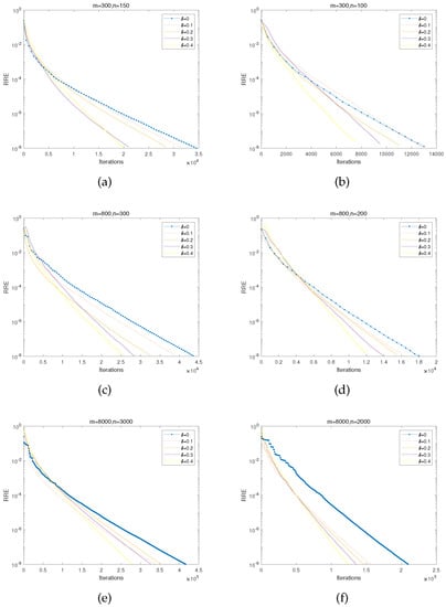
Figure 1. (a,b): m = 300 rows and n = 150, 100 columns for different $\delta$. (c,d): m = 800 rows and n = 300, 200 columns for different $\delta$. (e,f): m = 8000 rows and n = 3000, 2000 columns for different $\delta$.

4.2. Experiments for NARCD, RCDm, RCD, NASGD

Matrix A is randomly generated by using the MATLAB function unifrnd (0,1,m,n). For the RCDm method, let us take the momentum parameter $\delta =0.3$. For the NARCD method, let us take the Nesterov accelerated parameter $\lambda =0.05$. For the Nesterov accelerated stochastic gradient descent method (NASGD), it is the step size $\alpha =0.01$. We observe the performances of RCD, RCDm, and NARCD methods with matrices A of different sizes. From Figure 2 and Table 4, Table 5, Table 6 and Table 7, we found that both the NARCD and the RCDm with appropriate momentum parameters can accelerate the RCD; the NARCD and the RCDm always converge faster than the RCD. Moreover, we found that the NARCD has a better acceleration effect than the RCDm. From Table 7, for matrix A $\in R^{8000\times 3000}$, the NARCD method demonstrates the best numerical results than the other matrices in terms of the value of the speed-up, where the speed-up is $3.0206$. From Figure 3, we found that the acceleration of NARCD method and RCDm method experience gentle changes as the matrix becomes larger, so we can see that these two methods still have good speed-ups when the matrix is very large. From Figure 4, we found that the NARCD converges faster than the NASGD.

Figure 2. (a,b): m = 4000 rows and n = 800, 1000 columns for RCD, RCDm, and NARCD. (c,d): m = 8000 rows and n = 2000, 3000 columns for RCD, RCDm, and NARCD. (e,f): m = 12,000 rows and n = 2000, 4000 columns for RCD, RCDm, and NARCD.

Table 4. IT and CPU of RCD, RCDm, NARCD for matrices $A\in R^{m\times n}$ with m = 4000 and different n.

	IT		CPU
	$\mathbf{4000}\times \mathbf{800}$	$\mathbf{4000}\times \mathbf{1000}$	$\mathbf{4000}\times \mathbf{800}$	$\mathbf{4000}\times \mathbf{1000}$
RCD	57,723	81,926	1.3939	1.9264
RCDm	44,962	66,425	1.1068	1.5824
NARCD	20,075	24,184	0.8657	0.9711

Table 5. IT and CPU of RCD, RCDm, NARCD for matrices $A\in R^{m\times n}$ with m = 8000 and different n.

	IT		CPU
	$\mathbf{8000}\times \mathbf{2000}$	$\mathbf{8000}\times \mathbf{3000}$	$\mathbf{8000}\times \mathbf{2000}$	$\mathbf{8000}\times \mathbf{3000}$
RCD	194,046	414,465	9.4357	24.2728
RCDm	144,592	312,665	8.0861	19.1512
NARCD	45,700	71,216	4.5801	8.0357

Table 6. IT and CPU of RCD, RCDm, NARCD for matrices $A\in R^{m\times n}$ with m = 12,000 and different n.

	IT		CPU
	12,000 × 2000	12,000 × 4000	12,000 × 2000	12,000 × 4000
RCD	146,007	465,484	10.8746	31.4180
RCDm	110,339	340,633	8.5894	23.4675
NARCD	43,110	89,046	5.7312	11.0535

Table 7. The speed-up of the RCD method against the NARCD and RCDm.

	$4000\times 1000$	$8000\times 3000$	12,000 $\times 4000$
$speed-u{p}_1$	1.2173	1.2674	1.3387
$speed-u{p}_2$	1.9837	3.0206	2.8423

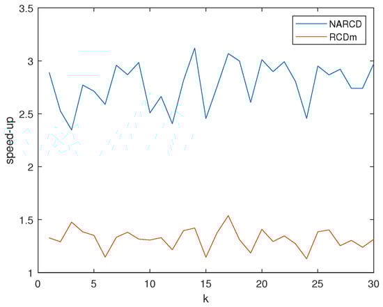
Figure 3. The speed-up of the RCD method against the NARCD and RCDm for matrices $A\in R^{m\times n}$ with $m=300\times k$ and $n=100\times k$.

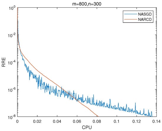
Figure 4. m = 800 and n = 300 for NARCD and NASGD.

4.3. Experiment with Different Correlations of Matrix A

Matrix A is randomly generated by using the MATLAB function unifrnd (c,1,m,n), $c\in [0,1)$. We let $c=0,0.2,0.4,0.6$. For the RCDm method, let us take the momentum parameter $\delta =0.3$. For the NARCD method, let us take the Nesterov accelerated parameter $\lambda =0.05$. As the value of c increases, the correlation of matrix A becomes stronger. From Table 8, Table 9, Table 10, Table 11 and Table 12, we know that as c increases, the condition number for the matrix increases. The larger the condition number, the more ill-conditioned the matrix. The more ill-conditioned the matrix, the more time it takes to solve. From Table 10 and Table 12, we know that the acceleration effect of RCDm does not change much with the increase of the c value, but the acceleration effect of NARCD is becoming better.

Table 8. The condition number of different matrices.

	0	$0.2$	$0.4$	$0.9$
$cond\left(A_{800\times 300}\right)$	75.6431	113.8689	172.7404	1425.0834
$cond\left(A_{1000\times 800}\right)$	452.9536	673.9111	1104.0601	8969.5561

Table 9. IT and CPU of RCD, RCDm, NARCD for matrices $A\in R^{m\times n}$ m = 800, n = 300.

	IT				CPU
	0	$0.2$	$0.4$	$0.9$	0	$0.2$	$0.4$	$0.9$
RCD	34,953	68,289	150,982	-	0.1993	0.4009	0.9189	-
RCDm	30,908	54,842	120,490	4,374,385	0.1715	0.3642	0.6787	24.3558
NARCD	8921	14,960	25,714	469,083	0.0708	0.1148	0.2134	3.5497

Table 10. The speed-up of the RCD method against the NARCD and RCDm, $A\in R^{m\times n}$ m = 800, n = 300.

	0	$0.2$	$0.4$	$0.9$
$speed-u{p}_1$	1.1620	1.1007	1.3539	-
$speed-u{p}_2$	2.5291	3.4921	4.3059	-

Table 11. IT and CPU of RCD, RCDm, NARCD for matrices $A\in R^{m\times n}$ m = 1000, n = 800.

	IT				CPU
	0	$\mathbf{0}.\mathbf{2}$	$\mathbf{0}.\mathbf{4}$	$\mathbf{0}.\mathbf{9}$	0	$\mathbf{0}.\mathbf{2}$	$\mathbf{0}.\mathbf{4}$	$\mathbf{0}.\mathbf{9}$
RCD	1,111,363	1,694,262	3,609,833	-	8.0508	11.9815	25.3595	-
RCDm	746,948	1,128,363	2,190,455	-	5.0748	7.7701	15.2623	-
NARCD	90,521	145,186	209,795	1,123,632	0.8005	1.0775	1.8670	10.4081

Table 12. The speed-up of the RCD method against the NARCD and RCDm, $A\in R^{m\times n}$ m = 1000, n = 800.

	0	$0.2$	$0.4$	$0.9$
$speed-u{p}_1$	1.5864	1.5420	1.6615	-
$speed-u{p}_2$	10.0572	11.1197	13.5830	-

4.4. The Two-Dimensional Tomography Test Problems

In this section, we use the previously and newly proposed methods to reconstruct 2D seismic travel time tomography. The 2D seismic travel-time tomography reconstruction is implemented in the function seismictomo (N, s, p) in the MATLAB package AIR TOOLS [29], which generated a sparse matrix A, an exact solution $x_{\ast }$(which is shown in Figure 4a) and the right vector $b+ϵ=A{x}^{\ast }+ϵ$ where $ϵ\in N\left(A^T\right)$. We set N = 20, s = 30 and p = 100 in the function seismictomo (N, s, p). We utilize the RCD, RCDm($\delta$=0.3) and NARCD($\lambda =0.05$) methods to solve the linear least-squares problem (1). The experiment ran 90,000 iterations. From Figure 5, we see that the results of the NARCD methods are better than those of the RCD and RCDm methods under the same number of iteration steps.

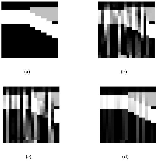
Figure 5. Performance of RCD, RCDm, and NARCD methods for the seismictomo test problem. (a) Exact seismic. (b) RCD. (c) RCDm. (d) NARCD.

5. Conclusions

To solve a large system of linear equations, two new acceleration methods for the RCD method are proposed, called the NARCD method and the RCDm method. Their convergences were proved, and the estimations of the convergence rates of the NARCD method and the RCDm method are given, respectively. The two methods are shown to be equally successful in numerical experiments. In uniformly distributed data, with appropriately chosen momentum parameters, the RCDm is better than the RCD in IT and CPU. The NARCD and the RCDm are faster than the RCD, and the NARCD has a better acceleration effect than the RCDm. In the case of an overdetermined linear system, for the NARCD method, the fatter the matrix, the better the acceleration. The acceleration effect of NARCD becomes better when c in the MATLAB function unifrnd (c, 1, m,n) increases. The block coordinate descent method is a very efficient method for solving large linear equations; in future work, it would be interesting to apply the two accelerated formats to the block coordinate descent method.

References

- Leventhal, D.; Lewis, A.S. Randomized methods for linear constraints: Convergence rates and conditioning. Math. Oper. Res. 2010, 35, 641–654. [Google Scholar] [CrossRef]
- Ruhe, A. Numerical aspects of Gram-Schmidt orthogonalization of vectors. Linear Algebra Its Appl. 1983, 52, 591–601. [Google Scholar] [CrossRef]
- Breheny, P.; Huang, J. Coordinate descent algorithms for nonconvex penalized regression, with applications to biological feature selection. Ann. Appl. Stat. 2011, 5, 232. [Google Scholar] [CrossRef]
- Chang, K.W.; Hsieh, C.J.; Lin, C.J. Coordinate descent method for large-scale l2-loss linear support vector machines. J. Mach. Learn. Res. 2008, 9, 1369–1398. [Google Scholar]
- Canutescu, A.A.; Dunbrack Jr, R.L. Cyclic coordinate descent: A robotics algorithm for protein loop closure. Protein Sci. 2003, 12, 963–972. [Google Scholar] [CrossRef] [PubMed]
- Bouman, C.A.; Sauer, K. A unified approach to statistical tomography using coordinate descent optimization. IEEE Trans. Image Process. 1996, 5, 480–492. [Google Scholar] [CrossRef] [PubMed]
- Ye, J.C.; Webb, K.J.; Bouman, C.A.; Millane, R.P. Optical diffusion tomography by iterative-coordinate-descent optimization in a Bayesian framework. JOSA A 1999, 16, 2400–2412. [Google Scholar] [CrossRef]
- Bai, Z.Z.; Wu, W.T. On greedy randomized coordinate descent methods for solving large linear least-squares problems. Numer. Linear Algebra Appl. 2019, 26, e2237. [Google Scholar] [CrossRef]
- Zhang, J.; Guo, J. On relaxed greedy randomized coordinate descent methods for solving large linear least-squares problems. Appl. Numer. Math. 2020, 157, 372–384. [Google Scholar] [CrossRef]
- Lu, Z.; Xiao, L. On the complexity analysis of randomized block-coordinate descent methods. Math. Program. 2015, 152, 615–642. [Google Scholar] [CrossRef]
- Necoara, I.; Nesterov, Y.; Glineur, F. Random block coordinate descent methods for linearly constrained optimization over networks. J. Optim. Theory Appl. 2017, 173, 227–254. [Google Scholar] [CrossRef]
- Richtárik, P.; Takáč, M. Iteration complexity of randomized block-coordinate descent methods for minimizing a composite function. Math. Program. 2014, 144, 1–38. [Google Scholar] [CrossRef]
- Karczmarz, S. Angenaherte auflosung von systemen linearer glei-chungen. Bull. Int. Acad. Pol. Sic. Let. Cl. Sci. Math. Nat. 1937, 35, 355–357. [Google Scholar]
- Strohmer, T.; Vershynin, R. A randomized Kaczmarz algorithm with exponential convergence. J. Fourier Anal. Appl. 2009, 15, 262–278. [Google Scholar] [CrossRef]
- Bai, Z.Z.; Wu, W.T. On greedy randomized Kaczmarz method for solving large sparse linear systems. SIAM J. Sci. Comput. 2018, 40, A592–A606. [Google Scholar] [CrossRef]
- Bai, Z.Z.; Wu, W.T. On relaxed greedy randomized Kaczmarz methods for solving large sparse linear systems. Appl. Math. Lett. 2018, 83, 21–26. [Google Scholar] [CrossRef]
- Liu, Y.; Gu, C.Q. Variant of greedy randomized Kaczmarz for ridge regression. Appl. Numer. Math. 2019, 143, 223–246. [Google Scholar] [CrossRef]
- Guan, Y.J.; Li, W.G.; Xing, L.L.; Qiao, T.T. A note on convergence rate of randomized Kaczmarz method. Calcolo 2020, 57, 1–11. [Google Scholar] [CrossRef]
- Du, K.; Gao, H. A new theoretical estimate for the convergence rate of the maximal weighted residual Kaczmarz algorithm. Numer. Math. Theory Methods Appl. 2019, 12, 627–639. [Google Scholar]
- Yang, X. A geometric probability randomized Kaczmarz method for large scale linear systems. Appl. Numer. Math. 2021, 164, 139–160. [Google Scholar] [CrossRef]
- Nesterov, Y. A method for unconstrained convex minimization problem with the rate of convergence O (1/k2). Dokl. Akad. Nauk Sssr 1983, 269, 543–547. [Google Scholar]
- Nesterov, Y. Efficiency of coordinate descent methods on huge-scale optimization problems. SIAM J. Optim. 2012, 22, 341–362. [Google Scholar] [CrossRef]
- Polyak, B.T. Some methods of speeding up the convergence of iteration methods. Ussr Comput. Math. Math. Phys. 1964, 4, 1–17. [Google Scholar] [CrossRef]
- Sun, T.; Li, D.; Quan, Z.; Jiang, H.; Li, S.; Dou, Y. Heavy-ball algorithms always escape saddle points. arXiv 2019, arXiv:1907.09697. [Google Scholar]
- Sarowar Morshed, M.; Saiful Islam, M. Accelerated Sampling Kaczmarz Motzkin Algorithm for The Linear Feasibility Problem. J. Glob. Optim. 2019, 77, 361–382. [Google Scholar] [CrossRef]
- Liu, J.; Wright, S. An accelerated randomized Kaczmarz algorithm. Math. Comput. 2016, 85, 153–178. [Google Scholar] [CrossRef]
- Loizou, N.; Richtárik, P. Momentum and stochastic momentum for stochastic gradient, newton, proximal point and subspace descent methods. Comput. Optim. Appl. 2020, 77, 653–710. [Google Scholar] [CrossRef]
- Higham, D.J.; Higham, N.J. MATLAB Guide; SIAM: Philadelphia, PA, USA, 2016. [Google Scholar]
- Hansen, P.C.; Jørgensen, J.S. AIR Tools II: Algebraic iterative reconstruction methods, improved implementation. Numer. Algorithms 2018, 79, 107–137. [Google Scholar] [CrossRef]
Publisher’s Note: MDPI stays neutral with regard to jurisdictional claims in published maps and institutional affiliations. |
© 2022 by the authors. Licensee MDPI, Basel, Switzerland. This article is an open access article distributed under the terms and conditions of the Creative Commons Attribution (CC BY) license (https://creativecommons.org/licenses/by/4.0/).