Parameter Estimation for a Fractional Black–Scholes Model with Jumps from Discrete Time Observations

Abstract

We consider a stochastic differential equation (SDE) governed by a fractional Brownian motion $\left(B_t^H\right)$ and a Poisson process $\left(N_t\right)$ associated with a stochastic process $\left(A_t\right)$ such that: $d{X}_t=\mu X_{t}dt+\sigma X_{t}d{B}_t^H+A_t{X}_{t^{-}}d{N}_t,X_0=x_0>0.$ The solution of this SDE is analyzed and properties of its trajectories are presented. Estimators of the model parameters are proposed when the observations are carried out in discrete time. Some convergence properties of these estimators are provided according to conditions concerning the value of the Hurst index and the nonequidistance of the observation dates.

1. Introduction

Modeling with fractional Brownian motions is an interesting tool in many domains where self-similarity and short- or long-range dependence are evident. In this paper, we consider a stochastic differential equation (SDE) whose solutions are continuous-time stochastic processes that can be used in different applications such as finance or hydrology. It is an extension of the Black–Scholes model [1] in the case where there is a short- or long-term dependence with jumps of random amplitude. The main object of this paper is to provide estimation procedures for the extended model parameters.

Let $(\mathsf{\Omega },ℱ,{\left({ℱ}_t\right)}_{t\ge 0},\mathbb{P})$ be a filtered complete probability space. The SDE considered is:

$$d{X}_t=\mu X_{t}dt+\sigma X_{t}d{B}_t^H+A_t{X}_{t^{-}}d{N}_t,$$

(1)

where $\mu \in \mathbb{R}$ is the drift coefficient and $\sigma \in {\mathbb{R}}_{+}^{*}$ is the diffusion coefficient.

${\left(B_t^H\right)}_{t\ge 0}$ is the standard fBm with index $H\in (0,1)$ [2]. ${\left(N_t\right)}_{t\ge 0}$ is a homogeneous Poisson process with intensity $\lambda \in {\mathbb{R}}_{+}^{*}$. ${\left(A_t\right)}_{t\ge 0}$ is a stochastic process taking value in $(-1,+\infty )$. We assume that the three processes ${\left(N_t\right)}_{t\ge 0}$, ${\left(A_t\right)}_{t\ge 0}$ and ${\left(B_t^H\right)}_{t\ge 0}$ are independent and adapted to ${\left({ℱ}_t\right)}_{t\ge 0}$.

Our motivation is to propose parameter estimators for the solution $X={\left(X_t\right)}_{t\ge 0}$ of the SDE (1). Note that without the jump term $A_t{X}_{t^{-}}d{N}_t$, this SDE defines the Black–Scholes model governed by an fBm [3], which is one of the extensions of the mathematical model in finance introduced by [1]. One of these extensions is the mixed fractional SDE proposed by [4].

In the following, we denote by $ℳ(\mu ,{\sigma }^2,\lambda ,\theta ,x_0,H)$ the model followed by the solution of Equation (1) where $\theta \in {\mathbb{R}}^k$ stands for the distribution parameter of ${\left(A_t\right)}_{t\ge 0}$ and $x_0\in {\mathbb{R}}_{+}^{*}$ is the known initial value of ${\left(X_t\right)}_{t\ge 0}$. For an observation interval of length $T>0$, we focus on the estimation of $\mu ,{\sigma }^2,\lambda$ and $\theta$ from data consisting of observations of X on $(0,T]$ at n dates $0<t_1,\cdots ,t_n\le T$ plus the amplitude $A_{D_i}$ and the date $D_i$ of jumps for $i\in [1,N_T]\cap \mathbb{N}$. As in [5], we assume that the self-similarity parameter H is known. Nevertheless, procedures for estimating H such as quadratic variation methods [6] and regression methods [7] are discussed.

It is worth pointing out that statistical inference for fractional diffusion processes (without jumps) have been studied by many authors under discrete observations [3,8,9,10] and also under a continuous observation assumption [9]. They proposed estimation methods concerning mainly the drift and diffusion coefficients, but also sometimes the Hurst index H [3]. On the other hand, the Black–Scholes model with jumps governed by the standard Brownian motion was applied to hydrology data [11]. In this paper, we consider methods for estimating the drift and diffusion coefficients as well as the parameters of the jump distribution for a fractional Black–Scholes model with jumps. In Section 2, we first recall some properties of fBm and then present distributional properties of the solution of Equation (1). In Section 3, we propose estimators for the parameters of this fractional Black–Scholes process with jumps. Their asymptotic properties are studied. Procedures for simulating $ℳ(\mu ,{\sigma }^2,\lambda ,\theta ,x_0,H)$ are provided in Section 4 with numerical codes given in Appendix A. Section 5 proposes some perspectives for future work.

2. Preliminaries

The standard fractional Brownian motion ${\left(B_t^H\right)}_{t\in \mathbb{R}}$ with Hurst index $H\in (0,1)$ is a continuous and centered Gaussian process with covariance function [12]:

$$\mathbb{E}\left(B_s^H{B}_t^H\right)=\frac{1}{2}\left({\left|s\right|}^{2H}+{\left|t\right|}^{2H}-{|s-t|}^{2H}\right),\forall (s,t)\in {\mathbb{R}}^2.$$

(2)

Thus, $B_t^H$ follows a Gaussian distribution with parameters $(0,|t{|}^{2H})$. In the following, we consider the restriction of the fBm on ${\mathbb{R}}_{+}$. The process ${\left(B_t^H\right)}_{t\ge 0}$ has stationary increments but these increments are dependent unless $H=\frac{1}{2}$. In this last case, we get the standard Brownian motion. We have a long-term dependence when $H\in (\frac{1}{2},1)$ and a positive correlation between increments. Inversely, the increments are negatively correlated when $H\in (0,\frac{1}{2})$. Nevertheless, long-range dependence with a positive correlation is usually considered in practice for more realistic modeling. More detailed properties of fBm can be seen in [2,12,13]. Note the pioneering work of [14] and their discussion of potential applications of fBm for modeling long-term dependence in economics or hydrology.

Lemma 1.

Let $T\in {\mathbb{R}}_{+}^{*}$ and ${\left(X_t\right)}_{t\in {\mathbb{R}}^{+}}$ be a solution of SDE (1), then

$$\forall t\in (0,T],X_t=\left\{\begin{array}{cc}(1+A_t)X_{t^{-}}& \mathit{if}t\in \{D_1,\cdots ,D_{N_T}\}\\ & \\ X_{t^{-}}& \mathrm{otherwise}\end{array}\right.$$

(3)

where ${\displaystyle X_{t^{-}}=\underset{\stackrel{s\to t}{s<t}}{lim}{X}_s}$.

Proof. 

Note that the fractional Black–Scholes process without jump has continuous trajectories since the fBm is continuous. When jumps are included in the model, the process trajectories are continuous on any open interval $(D_i,D_{i+1})$ between two consecutive jump dates. Furthermore, from Equation (1), we can write

$$\forall (t,ϵ)\in (0,T]\times {\mathbb{R}}_{+}^{*},X_t-X_{t-ϵ}=\mu {\int }_{t-ϵ}^t{X}_{s^{-}}ds+\sigma {\int }_{t-ϵ}^t{X}_{s^{-}}d{B}_s^H+{\int }_{t-ϵ}^t{A}_s{X}_{s^{-}}d{N}_s$$

(4)

where ${\displaystyle {\int }_{t-ϵ}^t{A}_s{X}_{s}d{N}_s=\sum _{i\in (N_{t-ϵ},N_t]}{A}_{D_i}{X}_{D_i^{-}}}$. When $ϵ$ tends to zero, we get

$$X_t-X_{t^{-}}=\sum _{i\in (N_{t^{-}},N_t]}{A}_{D_i}{X}_{D_i^{-}}=\left\{\begin{array}{cc}{A}_t{X}_{t^{-}}& \mathrm{if}t\in \{D_1,\cdots ,D_{N_T}\}\\ & \\ 0& \mathrm{otherwise}\end{array}.\right.$$

This leads us to the final result.    □

This lemma emphasizes that $A_t$ is the relative jump at date t while the raw jump at t, which is $X_t-X_{t^{-}}$, is equal to $A_t{X}_{t^{-}}$.

We have not ruled out in our model the fact of having jumps with negative values. For example, consider that $1+A_t$ follows a log-Gaussian distribution denoted by $ℒ𝒩({\theta }_{1,t},{\theta }_{2,t})$. This means that ${\theta }_{1,t}$ and ${\theta }_{2,t}$ are the expectation and variance of $log(1+A_t)$, respectively. In such a case, $A_t$ may take negative values since

$$\mathbb{P}\left(A_t\in (-1,0]\right)=\mathbb{P}\left(log(1+A_t)\in (-\infty ,0]\right)=\mathsf{\Phi }\left(-{\displaystyle \frac{{\theta }_{1,t}}{\sqrt{{\theta }_{2,t}}}}\right)>0$$

(5)

where $\mathsf{\Phi }$ is the standard normal cumulative distribution function.

Theorem 1.

The solution of Equation (1) is given by:

$$\forall t\in {\mathbb{R}}_{+},X_t=X_{0}exp\left(\mu t-\frac{1}{2}{\sigma }^2{t}^{2H}+\sigma B_t^H+{\int }_0^{t}log(1+A_s)d{N}_s\right)$$

(6)

Proof. 

To solve SDE (1), we can proceed in two steps. Firstly, we consider SDE (7) without jumps associated with SDE (1):

$$d{X}_t=\mu X_{t}dt+\sigma X_{t}d{B}_t^H,X_0=x_0>0$$

(7)

By applying to SDE (7) the stochastic integrating method proposed by [15] for SDEs driven by a fractional Brownian motion, we get:

$$\forall t\in {\mathbb{R}}_{+},X_t=X_{0}exp\left(\mu t+\sigma B_t^H-\frac{1}{2}{\sigma }^2{t}^{2H}\right).$$

(8)

Secondly, we take into consideration the fact there is no jump in any open interval between two consecutive jump dates. For any given t in ${\mathbb{R}}_{+}$, we can write

$$[0,t]=\left(\bigcup _{i=1}^{N_t}[D_{i-1},D_i)\right)\cup \left\{D_{N_t}\right\}\cup (D_{N_t},t]\mathrm{with}{D}_0=0.$$

According to Equality (8), conditional on $X_0=x_0$, we have

$$\forall s\in [0,D_1),X_s=x_{0}exp(\mu s+\sigma B_s^H-\frac{1}{2}{\sigma }^2{s}^{2H}).$$

(9)

Therefore,

$$X_{D_1^{-}}=\underset{\stackrel{t\to D_1}{t<D_1}}{lim}{X}_t=x_{0}exp(\mu D_1+\sigma B_{D_1}^H-\frac{1}{2}{\sigma }^2{D}_1^{2H})$$

(10)

and from Lemma 1, we get

$$X_{D_1}=x_0(1+A_{D_1})exp(\mu D_1+\sigma B_{D_1}^H-\frac{1}{2}{\sigma }^2{D}_1^{2H}).$$

(11)

On the other hand, Lemma 1 gives us

$$\forall i\in [1,N_t]\cap \mathbb{N},X_{D_i}=(1+A_{D_i})X_{D_i^{-}}.$$

Consequently, for $1<i\le N_t$, we obtain in a similar way as above

$$\forall s\in [D_{i-1},D_i),X_s=x_0\prod _{j=1}^{i-1}(1+A_{D_j})exp(\mu s+\sigma B_s^H-\frac{1}{2}{\sigma }^2{s}^{2H}).$$

(12)

and

$$X_{D_i}=x_0\prod _{j=1}^i(1+A_{D_j})exp(\mu D_i+\sigma B_{D_i}^H-\frac{1}{2}{\sigma }^2{D}_i^{2H}).$$

(13)

Thus, for $s\in (D_{N_t},t]$,

$$X_s=x_0\prod _{i=1}^{N_t}(1+A_{D_i})exp(\mu s+\sigma B_s^H-\frac{1}{2}{\sigma }^2{s}^{2H}).$$

Since

$$\prod _{i=1}^{N_t}(1+A_{D_i})=exp\left({\int }_0^{t}log(1+A_s)d{N}_s\right),$$

Equations (9)–(13) lead us to the final result.    □

Proposition 1.

Consider the process ${\left(X_t\right)}_{t\ge 0}$ defined by Equation (6) and suppose that the following three conditions are verified:

$\mathit{\left(}C1\mathit{\right)}$

The processes ${\left(N_t\right)}_{t\ge 0}$, ${\left(A_t\right)}_{t\ge 0}$ and ${\left(B_t^H\right)}_{t\ge 0}$ are independent;

$\mathit{\left(}C2\mathit{\right)}$

$\forall i\in [1,N_t]\cap \mathbb{N},\mathbb{E}\left(A_{D_i}^2\right)<\infty$;

$\mathit{\left(}C3\mathit{\right)}$

For any $t>0$, the random variables $A_{D_i},i=1,\cdots ,N_t$ are independent and identically distributed.

Then, for $(t,x_0)\in {\mathbb{R}}_{+}\times \mathbb{R}$, conditionally to $X_0=x_0$,

$\mathit{\left(}i\mathit{\right)}$

The expectation of $X_t$ is

$$\mathbb{E}\left(X_t\right|X_0=x_0)=x_{0}exp\left(\left(\mu +\lambda \mathbb{E}\left(A_{D_1}\right)\right)t\right);$$

(14)

$\mathit{\left(}ii\mathit{\right)}$

The variance of $X_t$ is

$$Var\left(X_t\right|X_0=x_0)={\mathbb{E}}^2\left(X_t\right|X_0=x_0)\left(exp\left({\sigma }^2{t}^{2H}+\lambda t\mathbb{E}\left(A_{D_1}^2\right)\right)-1\right).$$

(15)

Proof. 

(i)

Equation (6) leads to the expectation of $X_t$ conditionally to $X_0=x_0$:

$\mathbb{E}\left(X_t\right|X_0=x_0)=x_{0}exp(\mu t-\frac{1}{2}{\sigma }^2{t}^{2H})\times \mathbb{E}\left(e^{\sigma B_t^H}\times exp\left({\int }_0^{t}log(1+A_s)d{N}_s\right)\right).$

Since condition $\left(C1\right)$ is verified, then

$$\begin{array}{ccc}\hfill \mathbb{E}\left(X_t\right|X_0=x_0)& =& x_{0}exp(\mu t-\frac{1}{2}{\sigma }^2{t}^{2H})\times exp\left(\frac{1}{2}{\sigma }^2{t}^{2H}\right)\times \mathbb{E}\left(\prod _{i=1}^{N_t}(1+A_{D_i})\right)\hfill \\ & =& x_{0}exp\left(\mu t\right)\times \mathbb{E}\left[{\left(1+\mathbb{E}\left(A_{D_1}\right|N_t)\right)}^{N_t}\right](\mathrm{because}\mathrm{of}\left(C3\right)).\hfill \end{array}$$

The independence of $A_{D_1}$ and $N_t$ implies that $\mathbb{E}\left(A_{D_1}\right|N_t)=\mathbb{E}\left(A_{D_1}\right)$ and then

$$\begin{array}{ccc}\hfill \mathbb{E}\left(X_t\right|X_0=x_0)& =& x_{0}exp\left(\mu t\right)\times \mathbb{E}\left[{\left(1+\mathbb{E}\left(A_{D_1}\right)\right)}^{N_t}\right]\hfill \\ & =& x_{0}exp\left(\mu t\right)\times exp\left(\lambda t(1+\mathbb{E}\left(A_{D_1}\right)-1)\right)\hfill \\ & =& x_{0}exp\left(\left(\mu +\lambda \mathbb{E}\left(A_{D_1}\right)\right)t\right).\hfill \end{array}$$

(ii)

Similarly, we get

$$\begin{array}{ccc}\hfill \mathbb{E}\left(X_t^2\right|X_0=x_0)& =& x_0^{2}exp(2\mu t-{\sigma }^2{t}^{2H})\times exp\left(2{\sigma }^2{t}^{2H}\right)\times \mathbb{E}\left(\prod _{i=1}^{N_t}{(1+A_{D_i})}^2\right)\hfill \\ & =& x_0^{2}exp(2\mu t+{\sigma }^2{t}^{2H})\times exp\left(\lambda t\left(2\mathbb{E}\left(A_{D_1}\right)+\mathbb{E}\left(A_{D_1}^2\right)\right)\right)\hfill \end{array}$$

so that $Var\left(X_t\right|X_0=x_0)={\mathbb{E}}^2\left(X_t\right|X_0=x_0)\left(exp\left({\sigma }^2{t}^{2H}+\lambda t\mathbb{E}\left(A_{D_1}^2\right)\right)-1\right)$.    □

Theorem 2.

Let ${\left(X_t\right)}_{t\in {\mathbb{R}}^{+}}$ be the solution of Equation (1). If $\mu +\lambda \mathbb{E}\left(A_{D_1}\right)<0$, then the expected process ${\left(\mathbb{E}\left(X_t\right)\right)}_{t\ge 0}$ converges to zero and we have the following results:

$\mathit{\left(}i\mathit{\right)}$

If $2H-1<0$ and $\mu <-\frac{\lambda }{2}\left(2(\mathbb{E}\left(A_{D_1}\right)+\mathbb{E}\left(A_{D_1}^2\right)\right)$, then $\left(X_t\right)$ converges in mean square to zero.

$\mathit{\left(}ii\mathit{\right)}$

If $2H-1=0$ and $\mu <-\frac{\lambda }{2}\left(2(\mathbb{E}\left(A_{D_1}\right)+\mathbb{E}\left(A_{D_1}^2\right)+{\sigma }^2\right)$ then $\left(X_t\right)$ converges in mean square to zero.

$\mathit{\left(}iii\mathit{\right)}$

If $2H-1>0$, there is no mean-square convergence.

Proof. 

From Equation (14), we have

$$\forall t\in {\mathbb{R}}^{+},\mathbb{E}\left(X_t\right|X_0=x_0)=x_{0}exp\left(\left(\mu +\lambda \mathbb{E}\left(A_{D_1}\right)\right)t\right).$$

Since $\mu +\lambda \mathbb{E}\left(A_{D_1}\right)<0$, then

$${\displaystyle \forall x_0\in \mathbb{R},\underset{t\to +\infty }{lim}\mathbb{E}\left(X_t\right|X_0=x_0)=0.}$$

On the other hand, let us write

$$R_t=2\mu +2\lambda \mathbb{E}\left(A_{D_1}\right)+\lambda \mathbb{E}\left(A_{D_1}^2\right)+{\sigma }^2{t}^{2H-1}.$$

Then,

$$\begin{array}{ccc}\hfill \mathbb{E}\left(X_t^2\right|X_0=x_0)& =& x_0^{2}exp\left(\left(2\mu +2\lambda \mathbb{E}\left(A_1\right)+\lambda \mathbb{E}\left(A_1^2\right)+{\sigma }^2{t}^{2H-1}\right)t\right)\hfill \\ & =& x_0^{2}exp\left(t{R}_t\right).\hfill \end{array}$$

$\left(i\right)$ If $2H-1<0$, then ${\displaystyle \underset{t\to +\infty }{lim}{R}_t=2\mu +2\lambda \mathbb{E}\left(A_1\right)+\lambda \mathbb{E}\left(A_1^2\right)<0}$ so that ${\displaystyle \underset{t\to +\infty }{lim}\mathbb{E}\left(X_t^2\right)=0}$.

$\left(ii\right)$ If $2H-1=0$ then ${\displaystyle \underset{t\to +\infty }{lim}{R}_t=2\mu +2\lambda \mathbb{E}\left(A_1\right)+\lambda \mathbb{E}\left(A_1^2\right)+{\sigma }^2<0}$ and ${\displaystyle \underset{t\to +\infty }{lim}\mathbb{E}\left(X_t^2\right)=0}$.

$\left(iii\right)$ If $2H-1>0$, then $t{R}_t=\left(\left(2\mu +2\lambda \mathbb{E}\left(A_1\right)+\lambda \mathbb{E}\left(A_1^2\right)\right)t^{1-2H}+{\sigma }^2\right)t^{2H}$ tends to infinity when t tends to infinity. Therefore, we do not have mean-square convergence to zero.    □

3. Parameter Estimation

In the case of SDEs without jumps, several parameter estimation methods have been discussed in the literature [3,5,9,16,17]. In this paper, our main goal is to estimate the parameters of model (6) which incorporates jumps. The process ${\left(X_t\right)}_{t\ge 0}$ is observed discretely on the interval $[0,T]$ at dates $t_1,\cdots ,t_n$ with $T>0$ and $0<t_1,\cdots ,t_n\le T$. The process ${\left(N_t\right)}_{t\ge 0}$ is fully observed on $[0,T]$ and each jump amplitude $A_{D_i}$ is available for $i\in [1,N_T]\cap \mathbb{N}$.

In the following, we write $Y_t=log\left(X_t\right)$ so that Equation (6) leads to:

$$Y_t=log\left(X_0\right)+\sum _{i=1}^{N_t}log(1+A_{D_i})+\mu t-\frac{1}{2}{\sigma }^2{t}^{2H}+\sigma B_t^H.$$

(16)

In Section 3.1, the maximum likelihood estimators (MLEs) of $\mu ,{\sigma }^2$ and $\lambda$ are provided assuming that $x_0$ and H are known. The estimation of the jump amplitude parameter $\theta$ is presented in Section 3.2. Then, an asymptotically unbiased and consistent estimator of ${\sigma }^2$ is proposed in Section 3.3 by means of quadratic variations. Results on convergence properties of MLEs are obtained in Section 3.4 with respect to the Hurst index value in situations where it is not necessary to assume the same interval length between two consecutive observation dates.

3.1. Maximum Likelihood Estimator of $(\mu ,{\sigma }^2,\lambda )$

As mentioned before, refs. [3,17] proposed a MLE in the case of SDEs without jumps. In the following theorem, we take into account the dates and amplitudes of jump to provide the MLE of $(\mu ,{\sigma }^2,\lambda )$.

Theorem 3.

The MLEs of $\mu ,{\sigma }^2$ and λ from the observations $Y_{t_1},\cdots ,Y_{t_n}$, $A_{D_1},\cdots ,A_{D_{N_t}}$ are, respectively,

$$\widehat{\mu }=\frac{{\displaystyle \sum _{i=1}^n\sum _{j=1}^n{t}_i{\mathsf{\Gamma }}_{ij}^{-1}\left(Y_{t_j}+\frac{1}{2}\widehat{{\sigma }^2}{t}_j^{2H}-log\left(X_0\right)-\sum _{k=1}^{N_{t_j}}log(1+A_{D_k})\right)}}{{\displaystyle \sum _{i=1}^n\sum _{j=1}^n{t}_i{t}_j{\mathsf{\Gamma }}_{ij}^{-1}}}$$

(17)

$$\widehat{{\sigma }^2}=2\frac{{\displaystyle {\left(n^2+\left(\sum _{i=1}^n\sum _{j=1}^n{C}_{t_i}{\mathsf{\Gamma }}_{ij}^{-1}{C}_{t_j}\right)\left(\sum _{i=1}^n\sum _{j=1}^n{t}_i^{2H}{t}_j^{2H}{\mathsf{\Gamma }}_{ij}^{-1}\right)\right)}^{1/2}-n}}{{\displaystyle \sum _{i=1}^n\sum _{j=1}^n{t}_i^{2H}{t}_j^{2H}{\mathsf{\Gamma }}_{ij}^{-1}}}$$

(18)

$$\widehat{\lambda }={\displaystyle \frac{N_T}{T}}$$

(19)

where the ${\mathsf{\Gamma }}_{ij}^{-1}$ are the elements of the inverse matrix ${\mathsf{\Gamma }}^{-1}$ of Γ with $\mathsf{\Gamma }=(\mathbb{E}\left(B_{t_i}^H{B}_{t_j}^H\right){)}_{\genfrac{}{}{0pt}{}{1\le i\le n}{1\le j\le n}}$ given by Equation (2).

                                       ${\displaystyle C_{t_i}=Y_{t_i}-\widehat{\mu }{t}_i-log\left(X_0\right)-\sum _{k=1}^{N_{t_i}}log(1+A_{D_k})}$.

Proof. 

The random variable $Y_t$ as defined in expression (16) has a Gaussian distribution conditionally to ${\left(A_{D_i}\right)}_{i=1,\cdots ,N_t}$ with expectation

$${\displaystyle \mathbb{E}\left(Y_t|{\left(A_{D_i}\right)}_{1\le i\le N_t},N_t\right)=log\left(x_0\right)+\sum _{i=1}^{N_t}log(1+A_{D_i})+\mu t-\frac{1}{2}{\sigma }^2{t}^{2H}}$$

(20)

and variance

$$Var\left(Y_t|{\left(A_{D_i}\right)}_{1\le i\le N_t},N_t\right)={\sigma }^2{t}^{2H}.$$

(21)

Writing $\mathit{t}=(t_1,\cdots ,t_n),{\mathit{t}}^{\mathbf{2}\mathit{H}}=(t_1^{2H},\cdots ,t_n^{2H}),\mathit{Y}=(Y_{t_1},\cdots ,Y_{t_n})$ and ${\displaystyle {\mathit{Z}}_{\mathit{t}}=\left(log\left(x_0\right)+\sum _{k=1}^{N_{t_1}}log(1+A_{D_k}),\cdots ,log\left(x_0\right)+\sum _{k=1}^{N_{t_n}}log(1+A_{D_k})\right)}$, the log-likelihood $\mathcal{L}(\mathit{Y};(\mu ,{\sigma }^2))$ for the observations $\mathit{Y}$ conditional on ${\left(A_{D_i}\right)}_{1\le i\le N_T}$, $N_T$ and X₀ is

$$-\frac{n}{2}log\left(2\pi \right)-\frac{1}{2}log\left(\right|{\sigma }^2\mathsf{\Gamma }\left|\right)-\frac{1}{2{\sigma }^2}\left(\mathit{Y}-\mu \mathit{t}+\frac{1}{2}{\sigma }^2{\mathit{t}}^{\mathbf{2}\mathit{H}}-{\mathit{Z}}_{\mathit{t}}\right){\mathsf{\Gamma }}^{-1}{\left(\mathit{Y}-\mu \mathit{t}+\frac{1}{2}{\sigma }^2{\mathit{t}}^{\mathbf{2}\mathit{H}}-{\mathit{Z}}_{\mathit{t}}\right)}^{\prime }$$

where $\mathsf{\Gamma }$ is the square matrix $\left(\mathbb{E}\right(B_{t_i}^H{B}_{t_j}^H\left)\right)$ and prime (${}^{\prime }$) denotes the vector transposition.

Therefore, $\mathcal{L}(\mathit{Y};(\mu ,{\sigma }^2))$ can be expressed as follows:

$$\begin{array}{c}\mathcal{L}(\mathit{Y};(\mu ,{\sigma }^2))=\hfill \\ -\frac{n}{2}log\left(2\pi \right)-\frac{1}{2}log\left(\right|{\sigma }^2\mathsf{\Gamma }\left|\right)-\frac{1}{2{\sigma }^2}\sum _{i=1}^n\sum _{j=1}^n\left(y_{t_i}-\mu t_i+\frac{1}{2}{\sigma }^2{t}_i^{2H}-log\left(x_0\right)-\sum _{k=1}^{N_{t_i}}log(1+A_k)\right)\times \\ \hfill {\mathsf{\Gamma }}_{ij}^{-1}\left(y_{t_j}-\mu t_j+\frac{1}{2}{\sigma }^2{t}_j^{2H}-log\left(x_0\right)-\sum _{k=1}^{N_{t_j}}log(1+A_k)\right).\end{array}$$

(22)

The derivatives of expression (22) with respect to $\mu$ and ${\sigma }^2$ lead to the MLEs $\widehat{\mu }$ and $\widehat{{\sigma }^2}$ as expressed in Equations (17) and (18).

On the other hand, the independence condition $\left(C1\right)$ implies that the term from the full likelihood related to $\lambda$ is ${\displaystyle exp\left({\int }_0^{T}log\left(\lambda \right)d{N}_s-{\int }_0^T\lambda ds\right)={\lambda }^{N_T}exp(-\lambda T)}$ so that the MLE of $\lambda$ is $\widehat{\lambda }={\displaystyle \frac{N_T}{T}}$.    □

It is worth noticing that $\widehat{\mu }$ and $\widehat{{\sigma }^2}$ have a matrix expression:

$$\widehat{\mu }={\displaystyle \frac{\mathit{t}{\mathsf{\Gamma }}^{-1}{\mathit{K}}^{\prime }}{\mathit{t}{\mathsf{\Gamma }}^{-1}{\mathit{t}}^{\prime }}},$$

(23)

$$\widehat{{\sigma }^2}=2{\displaystyle \frac{{\left(n^2+\left({\mathit{t}}^{\mathbf{2}\mathit{H}}{\mathsf{\Gamma }}^{-1}{\left({\mathit{t}}^{\mathbf{2}\mathit{H}}\right)}^{\prime }\right)\mathit{C}{\mathsf{\Gamma }}^{-1}{\mathit{C}}^{\prime }\right)}^{\frac{1}{2}}-n}{{\mathit{t}}^{\mathbf{2}\mathit{H}}{\mathsf{\Gamma }}^{-1}{\left({\mathit{t}}^{\mathbf{2}\mathit{H}}\right)}^{\prime }}},$$

(24)

where $\mathit{C}=(C_{t_1},\cdots ,C_{t_n})$ and $\mathit{K}=(K_{t_1},\cdots ,K_{t_n})$ with

$$K_{t_j}=Y_{t_j}+\frac{1}{2}\widehat{{\sigma }^2}{t}_j^{2H}-log\left(X_0\right)-\sum _{k=1}^{N_{t_j}}log(1+A_{D_k})\mathrm{for}1\le j\le n.$$

(25)

3.2. Estimation of $\theta$

The observed jump amplitudes $D_1,\cdots ,D_{N_T}$ provide us with a sample of independent realizations from the same distribution, say ${𝒟}_{\theta }$. Consequently, statistical inference on $\theta$ can be performed by means of classical tools [18]. For example, the package maxlik [19] uses different optimization routines in the statistical environment R for maximum likelihood estimations.

3.3. Quadratic Variation Method for Estimating ${\sigma }^2$

Ref. [3] proposed a quadratic variation method for estimating ${\sigma }^2$ in the case where there are no jumps and for which the observation dates are equidistant. Our goal in this subsection is to extend this method and provide an asymptotically unbiased estimator of ${\sigma }^2$ in the case of jumps and for observation dates not necessarily equidistant.

Theorem 4.

From the observations $Y_{t_1},\cdots ,Y_{t_n}$, $A_{D_1},\cdots ,A_{D_{N_t}}$, the quadratic variation method provides the following estimator of ${\sigma }^2$:

$$\widetilde{{\sigma }^2}={\displaystyle \frac{1}{n}}\sum _{i=0}^{n-1}{\displaystyle \frac{{\displaystyle {\left(Y_{t_{i+1}}-Y_{t_i}-\sum _{j=N_{t_i}+1}^{N_{t_{i+1}}}log(1+A_{D_j})\right)}^2}}{{\displaystyle {(t_{i+1}-t_i)}^{2H}}}}$$

(26)

with $t_0=0$.

For $H>\frac{1}{2}$, if $t_i=hi+{ϵ}_i$ for $i=1,\cdots ,n$ with $h>0$ and ${ϵ}_i=o\left(\frac{1}{n}\right)$, then the estimator $\widetilde{{\sigma }^2}$ is asymptotically unbiased and consistent for ${\sigma }^2$.

Proof. 

For any integer i such that $0\le i<n$, from Equation (16), we get

$$Y_{t_{i+1}}-Y_{t_i}=\sum _{j=N_{t_i}+1}^{N_{t_{i+1}}}log(1+A_{D_j})+\mu (t_{i+1}-t_i)-\frac{1}{2}{\sigma }^2(t_{i+1}^{2H}-t_i^{2H})+\sigma (B_{t_{i+1}}^H-B_{t_i}^H)$$

Therefore, for $H>\frac{1}{2}$, we obtain in a similar way as [3]:

$${\left(Y_{t_{i+1}}-Y_{t_i}-\sum _{j=N_{t_i}+1}^{N_{t_{i+1}}}log(1+A_{D_j})\right)}^2={\sigma }^2{\left(B_{t_{i+1}}^H-B_{t_i}^H\right)}^2+o\left({(t_{i+1}-t_i)}^{2H}\right)$$

(27)

so that

$$\begin{array}{cc}{\displaystyle \frac{1}{n}}\sum _{i=0}^{n-1}{\displaystyle \frac{{\displaystyle {\left(Y_{t_{i+1}}-Y_{t_i}-\sum _{j=N_{t_i}+1}^{N_{t_{i+1}}}log(1+A_{D_j})\right)}^2}}{{\displaystyle {(t_{i+1}-t_i)}^{2H}}}}=\hfill & \\ & \hfill {\sigma }^2\sum _{i=0}^{n-1}{\displaystyle \frac{{\left(B_{t_{i+1}}^H-B_{t_i}^H\right)}^2}{{\displaystyle n{(t_{i+1}-t_i)}^{2H}}}}+o\left(\frac{1}{n}\right).\end{array}$$

(28)

Taking the expectation of both members of Equality (28), we get

$$\mathbb{E}\left(\widetilde{{\sigma }^2}\right)={\sigma }^2+o\left(\frac{1}{n}\right)$$

(29)

so that $\widetilde{{\sigma }^2}$ is asymptotically unbiased.

On the other hand, we can prove that $\widetilde{{\sigma }^2}$ is consistent by first calculating its second-order moment:

$$\mathbb{E}\left({\left(\widetilde{{\sigma }^2}\right)}^2\right)=\frac{1}{n^2}\mathbb{E}{\left(\sum _{i=0}^{n-1}{\displaystyle \frac{{\displaystyle {\left(Y_{t_{i+1}}-Y_{t_i}-\sum _{j=N_{t_i}+1}^{N_{t_{i+1}}}log(1+A_{D_j})\right)}^2}}{{\displaystyle {(t_{i+1}-t_i)}^{2H}}}}\right)}^2.$$

(30)

From (30), we obtain

$$\begin{array}{c}{n}^2\mathbb{E}\left({\left(\widetilde{{\sigma }^2}\right)}^2\right)=\sum _{i=0}^{n-1}{\displaystyle \frac{{\displaystyle \mathbb{E}{\left(Y_{t_{i+1}}-Y_{t_i}-\sum _{j=N_{t_i}+1}^{N_{t_{i+1}}}log(1+A_{D_j})\right)}^4}}{{\displaystyle {(t_{i+1}-t_i)}^{4H}}}}+\hfill \\ {\displaystyle 2\sum _{0\le i<k}^{n-1}\mathbb{E}{\left({\displaystyle \frac{{\displaystyle {\left(Y_{t_{i+1}}-Y_{t_i}-\sum _{j=N_{t_i}+1}^{N_{t_{i+1}}}log(1+A_{D_j})\right)}^2}}{{\displaystyle {(t_{i+1}-t_i)}^{2H}}}}\times {\displaystyle \frac{{\displaystyle {\left(Y_{t_{k+1}}-Y_{t_k}-\sum _{j=N_{t_k}+1}^{N_{t_{k+1}}}log(1+A_{D_j})\right)}^2}}{{\displaystyle {(t_{k+1}-t_k)}^{2H}}}}\right)}^2.}\hfill \end{array}$$

Using Equality (27) leads to

$$\begin{array}{c}\sum _{i=0}^{n-1}{\displaystyle \frac{{\displaystyle \mathbb{E}{\left(Y_{t_{i+1}}-Y_{t_i}-\sum _{j=N_{t_i}+1}^{N_{t_{i+1}}}log(1+A_{D_j})\right)}^4}}{{\displaystyle {(t_{i+1}-t_i)}^{4H}}}}=\hfill \\ \sum _{i=0}^{n-1}\frac{\mathbb{E}{\left({\sigma }^2{\left(B_{t_{i+1}}^H-B_{t_i}^H\right)}^2+o{(t_{i+1}-t_i)}^{2H}\right)}^2}{{(t_{i+1}-t_i)}^{4H}}=n(3{\sigma }^4+o\left(1\right)).\hfill \end{array}$$

(31)

Moreover,

$$\begin{array}{c}\hfill {\displaystyle \sum _{0\le i<k}^{n-1}\mathbb{E}{\left({\displaystyle \frac{{\displaystyle {\left(Y_{t_{i+1}}-Y_{t_i}-\sum _{j=N_{t_i}+1}^{N_{t_{i+1}}}log(1+A_{D_j})\right)}^2}}{{\displaystyle {(t_{i+1}-t_i)}^{2H}}}}\times {\displaystyle \frac{{\displaystyle {\left(Y_{t_{k+1}}-Y_{t_k}-\sum _{j=N_{t_k}+1}^{N_{t_{k+1}}}log(1+A_{D_j})\right)}^2}}{{\displaystyle {(t_{k+1}-t_k)}^{2H}}}}\right)}^2= }\\ \hfill \frac{n(n-1)}{2}\left({\sigma }^4+o\left(1\right)\right).\end{array}$$

(32)

Thus, the results (29), (31) and (32) lead us to

$$Var\left(\widetilde{{\sigma }^2}\right)=\frac{2{\sigma }^4}{n}+o\left(\frac{1}{n}\right)$$

so that $Var\left(\widetilde{{\sigma }^2}\right)$ tends to zero as n tends to ∞.

Furthermore, from Chebyshev’s inequality, we get for any $ϵ>0$

$$\begin{array}{ccc}\hfill P\left(\right|\widetilde{{\sigma }^2}-{\sigma }^2|\ge ϵ)& \le & P\left(\right|\widetilde{{\sigma }^2}-\mathbb{E}\left(\widetilde{{\sigma }^2}\right)|+|\mathbb{E}\left(\widetilde{{\sigma }^2}\right)-{\sigma }^2|\ge ϵ)\hfill \end{array}$$

(33)

$$\begin{array}{ccc}& \le & {\displaystyle \frac{Var\left(\widetilde{{\sigma }^2}\right)}{{\left(ϵ-|\mathbb{E}\left(\widetilde{{\sigma }^2}\right)-{\sigma }^2|\right)}^2}}\hfill \end{array}$$

(34)

which tends to zero as n tends to ∞ and implies the consistency of $\widetilde{{\sigma }^2}$ for ${\sigma }^2$.    □

3.4. Asymptotic Properties of MLEs

In this subsection, we focus on some distributional properties of estimators of $\mu$ and ${\sigma }^2$.

Theorem 5.

When ${\sigma }^2$ is known,

$\mathit{\left(}i\mathit{\right)}$

The estimator $\widehat{\mu }$ of μ is unbiased.

$\mathit{\left(}ii\mathit{\right)}$

If $t_i=hi+{ϵ}_i$ for $i=1,\cdots ,n$ with $h>0$ and ${ϵ}_i=o\left(\frac{1}{n}\right)$, then $\widehat{\mu }$ converges in mean square to μ as $n⟶\infty$.

$\mathit{\left(}iii\mathit{\right)}$

$\widehat{\mu }$ follows a Gaussian distribution with expectation μ and variance ${\displaystyle {\displaystyle \frac{{\sigma }^2}{\mathit{t}{\mathsf{\Gamma }}^{-1}{\mathit{t}}^{\prime }}}}$.

Proof. 

$\left(i\right)$

Let us write ${\mathit{B}}^{\mathit{H}}=(B_{t_1}^H,\cdots ,B_{t_n}^H)$. From Equations (16) and (25), we have $\mathit{K}=\mu \mathit{t}+\sigma {\mathit{B}}^{\mathit{H}}$ and Equation (23) leads to

$$\widehat{\mu }={\displaystyle \frac{\mathit{t}{\mathsf{\Gamma }}^{-1}(\mu {\mathit{t}}^{\prime }+\sigma {\left({\mathit{B}}^{\mathit{H}}\right)}^{\prime })}{\mathit{t}{\mathsf{\Gamma }}^{-1}{\mathit{t}}^{\prime }}}=\mu +\sigma {\displaystyle \frac{\mathit{t}{\mathsf{\Gamma }}^{-1}{\left({\mathit{B}}^{\mathit{H}}\right)}^{\prime }}{\mathit{t}{\mathsf{\Gamma }}^{-1}{\mathit{t}}^{\prime }}}.$$

(35)

${\mathit{B}}^{\mathit{H}}$ is centered so that $\mathbb{E}\left(\widehat{\mu }\right)=\mu$.

$\left(ii\right)$

From Equation (35), we obtain the variance of $\widehat{\mu }$:

$$Var\left(\widehat{\mu }\right)=\mathbb{E}\left({(\widehat{\mu }-\mu )}^2\right)={\sigma }^2\mathbb{E}\left({\displaystyle \frac{\mathit{t}{\mathsf{\Gamma }}^{-1}{\mathit{B}}^{\mathit{H}}{\left({\mathit{B}}^{\mathit{H}}\right)}^{\prime }{\mathsf{\Gamma }}^{-1}{\mathit{t}}^{\prime }}{{\left(\mathit{t}{\mathsf{\Gamma }}^{-1}{\mathit{t}}^{\prime }\right)}^2}}\right).$$

Since $\mathsf{\Gamma }=\mathbb{E}\left({\mathit{B}}^{\mathit{H}}{\left({\mathit{B}}^{\mathit{H}}\right)}^{\prime }\right)$, we obtain

$$Var\left(\widehat{\mu }\right)={\displaystyle \frac{{\sigma }^2}{\mathit{t}{\mathsf{\Gamma }}^{-1}{\mathit{t}}^{\prime }}}.$$

(36)

${\mathsf{\Gamma }}^{-1}$ is symmetric positive definite which implies that

$$\mathit{t}{\mathsf{\Gamma }}^{-1}{\mathit{t}}^{\prime }\ge {\displaystyle \frac{\mathit{t}{\mathit{t}}^{\prime }}{{\gamma }_{max}}}$$

(37)

where ${\gamma }_{max}$ denotes the largest eigenvalue of $\mathsf{\Gamma }$.

Consequently,

$$Var\left(\widehat{\mu }\right)\le {\sigma }^2{\displaystyle \frac{{\gamma }_{max}}{\mathit{t}{\mathit{t}}^{\prime }}}.$$

(38)

On the other hand,

$$\mathit{t}{\mathit{t}}^{\prime }=\sum _{i=1}^n{(hi+{ϵ}_i)}^2={\displaystyle \frac{n(n+1)(2n+1)}{6}}{h}^2+2h\sum _{i=1}^{n}i{ϵ}_i+\sum _{i=1}^n{ϵ}_i^2.$$

Since ${ϵ}_i=o\left(\frac{1}{n}\right)$, we have ${\mathit{t}\mathit{t}}^{\prime }={\displaystyle \frac{h^2{n}^3}{3}}+o\left(\frac{1}{n}\right)$. Moreover, according to Gerschgorin’s theorem (see [20], chp. 8), we have

$${\displaystyle {\gamma }_{max}\le \underset{i=1,\cdots ,n}{max}\sum _{j=1}^n\left|{\mathsf{\Gamma }}_{ij}\right|\le \beta n{\left(nh+o\left(\frac{1}{n}\right)\right)}^{2H}}$$

(39)

with $\beta >0$. From Inequalities (38) and (39), we get

$$Var\left(\widehat{\mu }\right)\le {\sigma }^2\beta h^{-2}{n}^{2H-2}/3$$

so that $Var\left(\widehat{\mu }\right)$ converges to zero when n tends to infinity.

$\left(iii\right)$

The result is straightforward from expressions (35) and (36).    □

Theorem 6.

When μ is known,

$\mathit{\left(}i\mathit{\right)}$

${\left(\widehat{{\sigma }^2}\right)}^2$ follows a noncentral chi-square distribution.

Assume that the following conditions are verified:

$\mathit{\left(}C4\mathit{\right)}$

$H>\frac{3}{4}$;

$\mathit{\left(}C5\mathit{\right)}$

$\exists i_0\in {\mathbb{N}}^{*},\forall i\ge i_0$, $t_i>1$;

$\mathit{\left(}C6\mathit{\right)}$

$t_i=hi+{ϵ}_i$ for $i=1,\cdots ,n$ with $h>0$ and ${ϵ}_i=o\left(\frac{1}{n}\right)$.

Then,

$\mathit{\left(}ii\mathit{\right)}$

The estimator $\widehat{{\sigma }^2}$ of ${\sigma }^2$ is asymptotically unbiased.

$\mathit{\left(}iii\mathit{\right)}$

$\widehat{{\sigma }^2}$ converges in mean square to ${\sigma }^2$ as $n⟶\infty$.

Proof. 

(i)

From Equality (24), we get that ${\left(\widehat{{\sigma }^2}\right)}^2$ is a quadratic form of the Gaussian vector $\mathit{C}$ so that it follows a noncentral chi-square distribution (see Theorem 5.5 in [21]).

(ii)

From Equation (24), we have

$$\mathbb{E}\left({\left(\widehat{{\sigma }^2}\right)}^2\right)=\frac{4\mathbb{E}\left(\mathit{C}{\mathsf{\Gamma }}^{-1}{\mathit{C}}^{\prime }\right)}{{\mathit{t}}^{\mathbf{2}\mathit{H}}{\mathsf{\Gamma }}^{-1}{\left({\mathit{t}}^{\mathbf{2}\mathit{H}}\right)}^{\prime }}.$$

(40)

Since

$$\mathbb{E}\left(\mathit{C}{\mathsf{\Gamma }}^{-1}{\mathit{C}}^{\prime }\right)=\mathbb{E}\left(\mathit{C}\right){\mathsf{\Gamma }}^{-1}\mathbb{E}\left({\mathit{C}}^{\prime }\right)+tr\left({\mathsf{\Gamma }}^{-1}{\sigma }^2\mathsf{\Gamma }\right)=\frac{1}{4}{\sigma }^4{\mathit{t}}^{\mathbf{2}\mathit{H}}{\mathsf{\Gamma }}^{-1}{\left({\mathit{t}}^{\mathbf{2}\mathit{H}}\right)}^{\prime }+n{\sigma }^2,$$

then

$$\mathbb{E}\left({\left(\widehat{{\sigma }^2}\right)}^2\right)={\sigma }^4+{\displaystyle \frac{4n{\sigma }^2}{{\mathit{t}}^{\mathbf{2}\mathit{H}}{\mathsf{\Gamma }}^{-1}{\left({\mathit{t}}^{\mathbf{2}\mathit{H}}\right)}^{\prime }}}.$$

Similarly to Inequality (37), we get

$${\mathit{t}}^{\mathbf{2}\mathit{H}}{\mathsf{\Gamma }}^{-1}{\left({\mathit{t}}^{\mathbf{2}\mathit{H}}\right)}^{\prime }\ge {\displaystyle \frac{{\mathit{t}}^{\mathbf{2}\mathit{H}}{\left({\mathit{t}}^{\mathbf{2}\mathit{H}}\right)}^{\prime }}{{\gamma }_{max}}}.$$

(41)

From condition $\left(C6\right)$ and Inequalities (39) and (41), it follows that

$${\displaystyle \frac{4n{\sigma }^2}{{\mathit{t}}^{\mathbf{2}\mathit{H}}{\mathsf{\Gamma }}^{-1}{\left({\mathit{t}}^{\mathbf{2}\mathit{H}}\right)}^{\prime }}}\le {\displaystyle \frac{4n{\sigma }^2{\gamma }_{max}}{{\mathit{t}}^{\mathbf{2}\mathit{H}}{\left({\mathit{t}}^{\mathbf{2}\mathit{H}}\right)}^{\prime }}}\le {\displaystyle \frac{4\beta n^2{\sigma }^2{\left(nh+o\left(\frac{1}{n}\right)\right)}^{2H}}{{\displaystyle \sum _{i=1}^n{\left(ih+o\left(\frac{1}{n}\right)\right)}^{4H}}}}.$$

When conditions $\left(C4\right),\left(C5\right)$ and $\left(C6\right)$ are verified, we obtain

$${\displaystyle \sum _{i=1}^n{\left(ih+o\left(\frac{1}{n}\right)\right)}^{4H}=\sum _{i=0}^n{\left(ih\right)}^3+o\left(\frac{1}{n}\right)={\displaystyle \frac{n^2{(n+1)}^2{h}^3}{4}}+o\left(\frac{1}{n}\right)}$$

(42)

which leads to

$${\displaystyle \frac{4n{\sigma }^2}{{\mathit{t}}^{\mathbf{2}\mathit{H}}{\mathsf{\Gamma }}^{-1}{\left({\mathit{t}}^{\mathbf{2}\mathit{H}}\right)}^{\prime }}}\le 16{\sigma }^2\beta h^{2H-3}{n}^{2H-2}$$

(43)

so that the bias of ${\left(\widehat{{\sigma }^2}\right)}^2$ for ${\sigma }^4$ converges to zero when n tends to infinity.

Due to the preservation of the convergence in probability and the distribution by continuous mappings (see Lemmas 3.3 and 3.7 in [22]), we obtain the final result.

$\left(iii\right)$

From Equation (24), we have

$$Var\left({\left(\widehat{{\sigma }^2}\right)}^2\right)=\frac{16Var\left(\mathit{C}{\mathsf{\Gamma }}^{-1}{\mathit{C}}^{\prime }\right)}{{\left({\mathit{t}}^{\mathbf{2}\mathit{H}}{\mathsf{\Gamma }}^{-1}{\left({\mathit{t}}^{\mathbf{2}\mathit{H}}\right)}^{\prime }\right)}^2}$$

(44)

and since

$$\begin{array}{ccc}\hfill Var\left(\mathit{C}{\mathsf{\Gamma }}^{-1}{\mathit{C}}^{\prime }\right)& =& 2tr\left({\left({\mathsf{\Gamma }}^{-1}{\sigma }^2\mathsf{\Gamma }\right)}^2\right)+4\mathbb{E}\left(\mathit{C}\right){\mathsf{\Gamma }}^{-1}\left({\sigma }^2\mathsf{\Gamma }\right){\mathsf{\Gamma }}^{-1}\mathbb{E}\left({\mathit{C}}^{\prime }\right)\hfill \\ & =& 2n{\sigma }^4+{\sigma }^6{\mathit{t}}^{\mathbf{2}\mathit{H}}{\mathsf{\Gamma }}^{-1}{\left({\mathit{t}}^{\mathbf{2}\mathit{H}}\right)}^{\prime }\hfill \end{array}$$

we get

$$\begin{array}{ccc}\hfill Var\left({\left(\widehat{{\sigma }^2}\right)}^2\right)& =& \frac{16\left(2n{\sigma }^4+{\sigma }^6{\mathit{t}}^{\mathbf{2}\mathit{H}}{\mathsf{\Gamma }}^{-1}{\left({\mathit{t}}^{\mathbf{2}\mathit{H}}\right)}^{\prime }\right)}{{\left({\mathit{t}}^{\mathbf{2}\mathit{H}}{\mathsf{\Gamma }}^{-1}{\left({\mathit{t}}^{\mathbf{2}\mathit{H}}\right)}^{\prime }\right)}^2}\hfill \\ & =& \frac{32n{\sigma }^4}{{\left({\mathit{t}}^{\mathbf{2}\mathit{H}}{\mathsf{\Gamma }}^{-1}{\left({\mathit{t}}^{\mathbf{2}\mathit{H}}\right)}^{\prime }\right)}^2}+\frac{16{\sigma }^6}{{\mathit{t}}^{\mathbf{2}\mathit{H}}{\mathsf{\Gamma }}^{-1}{\left({\mathit{t}}^{\mathbf{2}\mathit{H}}\right)}^{\prime }}.\hfill \end{array}$$

It results from (43) that the right member of Equality (44) tends to zero as n tends to infinity.

□

4. Numerical Simulations

In order to simulate ${\left(X_t\right)}_{t\ge 0}$ given by Equation (6), it is first necessary to simulate the fBm. Different methods have been discussed in the literature to simulate fBm trajectories [23,24]. Thus, the packages $somebm$ and $longmemo$ have been available with the software environment for statistical computing and graphics [25]. With function $fbm$ of $somebm$, we can simulation a standard fBm on $[0,1]$.

To get a simulation on any interval $[a,b]$ with $a<b$, we created a subdivision of length n by writing $t_i=a+\frac{i}{n}(b-a)$ for $i=0,\cdots ,n$ and used the following equalities in law:

$$B_{t_i}^H-B_a^H\stackrel{\mathcal{L}}{=}{B}_{t_i-a}^H\stackrel{\mathcal{L}}{=}{B}_{\frac{i}{n}(b-a)}^H(\mathrm{stationary}\mathrm{increment}\mathrm{property}),$$

$$B_{\frac{i}{n}(b-a)}^H\stackrel{\mathcal{L}}{=}{(b-a)}^H{B}_{\frac{i}{n}}^H(\mathrm{self}-\mathrm{similarity}\mathrm{property})$$

so that

$$B_{t_i}^H\stackrel{\mathcal{L}}{=}{B}_a^H+{(b-a)}^H{B}_{\frac{i}{n}}^H.$$

(45)

Equation (45) allows us to simulate an fBm trajectory on $[a,b]$ from one on $[0,1]$. In Appendix A, an R script simulating the model $ℳ(\mu ,{\sigma }^2,\lambda ,\theta ,x_0,H)$ is provided. In what follows, this script was applied to different parameter values $(\mu ,{\sigma }^2,\lambda ,\theta ,x_0,H)$ with respect to the convergence conditions given in Theorem 2. The jump amplitudes were distributed according to a log-Gaussian law with log-expectation ${\theta }_1$ and log-variance ${\theta }_2$. Then, four cases were distinguished:

Case 1: $\mu <min\left(-\lambda \left(e^{{\theta }_1+\frac{{\theta }_2}{2}}-1\right);-\frac{\lambda }{2}\left(e^{2({\theta }_1+{\theta }_2)}-1\right)\right)$ and $H<\frac{1}{2}$,

Case 2: $\mu <min\left(-\lambda \left(e^{{\theta }_1+\frac{{\theta }_2}{2}}-1\right);-\frac{\lambda }{2}\left(e^{2({\theta }_1+{\theta }_2)}-1+{\sigma }^2\right)\right)$ and $H=\frac{1}{2}$,

Case 3: $\mu <-\lambda \left(e^{{\theta }_1+\frac{{\theta }_2}{2}}-1\right)$ and $H>\frac{1}{2}$,

Case 4: $\mu >-\lambda \left(e^{{\theta }_1+\frac{{\theta }_2}{2}}-1\right)$.

The latter case is the situation for which the expected process ${\left(\mathbb{E}\left(X_t\right)\right)}_{t\ge 0}$ tends to infinity.

Figure 1 and Figure 2 provide graphical representations of the simulated trajectories for each case. The expectation and variance of the jump amplitudes were $0.111$ and $0.012$, respectively. The probability of a negative amplitude was $0.159$ in accordance with Equation (5). These figures illustrate the convergence results given by Theorem 2, namely that in cases 1 to 3, we had convergence of the expected process, and divergence of this process in case 4.

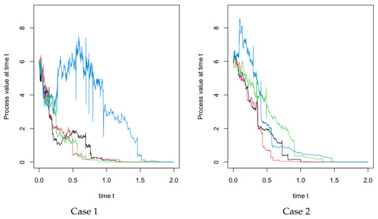
Figure 1. Four simulated trajectories of model $ℳ(\mu ,{\sigma }^2,\lambda ,\theta ,x_0,H)$ over $[0,2]$ for jumps distributed according to $\mathcal{LN}(0.1,0.01)$. On the left, an example of case 1 with $(\mu ,{\sigma }^2,\lambda ,\theta ,x_0,H)=(-1,0.2,5,(0.1,0.01),6,0.4)$; On the right, an example of case 2 with $(\mu ,{\sigma }^2,\lambda ,\theta ,x_0,H)=(-1,0.2,5,(0.1,0.01),6,0.5)$.

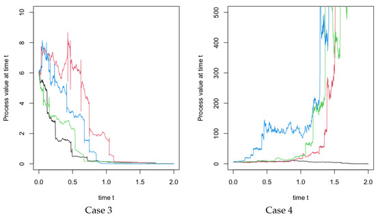
Figure 2. Four simulated trajectories of model $ℳ(\mu ,{\sigma }^2,\lambda ,\theta ,x_0,H)$ over $[0,2]$ for jumps distributed according to $\mathcal{LN}(0.1,0.01)$. On the left, an example of case 3 with $(\mu ,{\sigma }^2,\lambda ,\theta ,x_0,H)=(-1,0.2,5,(0.1,0.01),6,0.6)$; On the right, an example of case 4 with $(\mu ,{\sigma }^2,\lambda ,\theta ,x_0,H)=(0.1,0.2,5,(0.1,0.01),6,0.4)$.

Figure 3 illustrates the following theoretical result: between two consecutive jumps, the trajectories are smoother as H approaches unity and more irregular as H approaches zero.

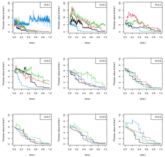
Figure 3. Four simulated trajectories of model $ℳ(-1,0.1,10,(0.1,0.01),6,H)$ over $[0,1]$ for H in $\{0.1,\dots ,0.9\}$. The trajectory smoothness between two consecutive jumps increases as H goes from 0 to 1.

5. Conclusions

Since the work of [14] on fractional noise, the fields of application of processes with long-term dependence have increased quite considerably. In this paper, we developed statistical inference for fractional Black–Scholes processes with jumps for which H is not necessarily greater than 1/2. First, the distributional properties of such processes were presented. Closed-form MLEs for the drift and diffusion coefficients were proposed. Their asymptotic properties were studied, in particular consistency. An asymptotically unbiased and consistent estimator of ${\sigma }^2$ was proposed by means of quadratic variations. These results were obtained with respect to the Hurst index value. Contrary to most methods proposed in the literature, we did not require an equal interval length between two consecutive observation dates. A procedure for simulating trajectories was developed within the programming environment.

We assumed independence between the Poisson process of jump dates and the series of jump amplitudes. It would be interesting in the future to study how the correlation between jump dates and amplitudes may impact the behavior of the SDE solution and the statistical inference on this process.

References

- Black, F.; Scholes, M.S. The Pricing of Options and Corporate Liabilities. J. Political Econ. 1973, 81, 637–654. [Google Scholar] [CrossRef]
- Biagini, F.; Hu, Y.; Øksendal, B.; Zhang, T. Stochastic Calculus for Fractional Brownian Motion and Applications; Springer Science & Business Media: London, UK, 2008. [Google Scholar]
- Xiao, W.; Zhang, W.; Zhang, X. Parameter identification for the discretely observed geometric fractional Brownian motion. J. Stat. Comput. Simul. 2015, 85, 269–283. [Google Scholar] [CrossRef]
- Shevchenko, G. Mixed fractional stochastic differential equations with jumps. Stochastics Int. J. Probab. Stoch. Process. 2014, 86, 203–217. [Google Scholar] [CrossRef]
- Bertin, K.; Torres, S.; Tudor, C.A. Maximum-likelihood estimators and random walks in long memory models. Statistics 2011, 45, 361–374. [Google Scholar] [CrossRef]
- Kubilius, K.; Melichov, D. Quadratic variations and estimation of the Hurst index of the solution of SDE driven by a fractional Brownian motion. Lith. Math. J. 2010, 50, 401–417. [Google Scholar] [CrossRef]
- Berzin, C.; León, J.R. Estimation in models driven by fractional Brownian motion. Ann. Inst. H. Poincaré Probab. Statist. 2008, 44, 191–213. [Google Scholar] [CrossRef]
- Hu, Y.; Nualart, D. Parameter estimation for fractional Ornstein–Uhlenbeck processes. Stat. Probab. Lett. 2010, 80, 1030–1038. [Google Scholar] [CrossRef]
- Mishura, Y.; Ralchenko, K.; Shklyar, S. Maximum likelihood estimation for Gaussian process with nonlinear drift. Nonlinear Anal. Model. Control. 2018, 23, 120–140. [Google Scholar] [CrossRef]
- Haress, E.M.; Hu, Y. Estimation of all parameters in the fractional Ornstein–Uhlenbeck model under discrete observations. Stat. Inference Stoch. Process. 2021, 24, 327–351. [Google Scholar] [CrossRef]
- Cesars, J.; Nuiro, S.; Vaillant, J. Statistical Inference on a Black-Scholes Model with Jumps. Application in Hydrology. J. Math. Stat. 2019, 15, 196–200. [Google Scholar] [CrossRef]
- Mishura, Y. Stochastic Calculus for Fractional Brownian Motion and Related Processes; Springer: Berlin/Heidelberg, Germany, 2008. [Google Scholar]
- Nualart, D. The Malliavin Calculus and Related Topics, 2nd ed.; Springer: Berlin/Heidelberg, Germany, 2006; Volume 1995. [Google Scholar]
- Mandelbrot, B.B.; Van Ness, J.W. Fractional Brownian motions, fractional noises and applications. SIAM Rev. 1968, 10, 422–437. [Google Scholar] [CrossRef]
- Unal, G.; Dinler, A. Exact linearization of one dimensional Itô equations driven by fBm: Analytical and numerical solutions. Nonlinear Dyn. 2008, 53, 251–259. [Google Scholar] [CrossRef]
- Mishura, Y.; Ralchenko, K.; Shklyar, S. Maximum likelihood drift estimation for Gaussian process with stationary increments. arXiv 2016, arXiv:1612.00160. [Google Scholar] [CrossRef]
- Yaozhong, H.; David, N.; Weilin, X.; Weiguo, Z. Exact maximum likelihood estimator for drift fractional Brownian motion at discrete observation. Acta Math. Sci. 2011, 31, 1851–1859. [Google Scholar] [CrossRef]
- Casella, G.; Berger, R.L. Statistical Inference; Cengage Learning: Belmont, CA, USA, 2021. [Google Scholar]
- Henningsen, A.; Toomet, O. maxLik: A package for maximum likelihood estimation in R. Comput. Stat. 2011, 26, 443–458. [Google Scholar] [CrossRef]
- Golub, G.H.; Van Loan, C.F. Matrix Computations; JHU Press: Baltimore, MD, USA, 2013. [Google Scholar]
- Rencher, A.C.; Schaalje, G.B. Linear Models in Statistics; John Wiley & Sons: Hoboken, NJ, USA, 2008. [Google Scholar]
- Kallenberg, O. Foundations of Modern Probability; Springer: Berlin/Heidelberg, Germany, 1997; Volume 2. [Google Scholar]
- Coeurjolly, J.F. Simulation and identification of the fractional Brownian motion: A bibliographical and comparative study. J. Stat. Softw. 2000, 5, 1–53. [Google Scholar] [CrossRef]
- Beran, J.; Whitcher, B.; Maechler, M. Longmemo: Statistics for Long-Memory Processes. 2009. Available online: http://CRAN.R-project.org/package=longmemo (accessed on 2 June 2020).
- R Core Team. R: A Language and Environment for Statistical Computing; R Foundation for Statistical Computing: Vienna, Austria, 2017. [Google Scholar]
Publisher’s Note: MDPI stays neutral with regard to jurisdictional claims in published maps and institutional affiliations. |
© 2022 by the authors. Licensee MDPI, Basel, Switzerland. This article is an open access article distributed under the terms and conditions of the Creative Commons Attribution (CC BY) license (https://creativecommons.org/licenses/by/4.0/).