Abstract
In classical continuum mechanics, a monolithic Eulerian formulation is used for numerically solving fluid–structure interaction (FSI) problems in the frame of a physically deformed configuration. This numerical approach is well adapted to large-displacement fluid–structure configurations where velocities of solids and fluids are computed all at once in a single variational equation. In the recent past, a monolithic Eulerian formulation for solving FSI problems of finite deformation to study the different physical features of fluid flow has been employed. Almost all the current studies use a classical framework in their approach. Despite producing decent results, such methods still need to be appropriately configured to generate exceptional results. Recently, a number of researchers have used a non-classical framework in their approach to analyze several physical problems. Therefore, in this paper, a monolithic Eulerian formulation is employed for solving FSI problems in a non-classical framework to study the micro-structural characteristics of fluid flow by validating the results with classical benchmark solutions present in the literature. In this respect, the Cosserat theory of continuum is considered where a continuum of oriented rigid particles has, in addition to the three translational degrees of freedom of classical continuum, three micro-rotational degrees of freedom. The mathematical formulation of model equations is derived from the general laws of continuum mechanics. Based on the variational formulation of the FSI system, we propose the finite element method and semi-implicit scheme for discretizing space and time domains. The results are obtained by computing a well-known classical FSI benchmark test problem FLUSTRUK-FSI-3* with FreeFem++. The results of the study indicate that the increase in micro-rotational viscosity leads to significantly large micro-rotations in fluid flow at the micro-structural level. Further, it is found that the amplitude of oscillations is related inversely to the material parameters c1 and while the increase in c1 stabilizes the amplitude of oscillations relatively more quickly than increasing The color snapshots of the numerical results at different times during the computer simulations and general conclusions drawn from the results are presented.
Keywords:
monolithic Eulerian formulation; Cosserat continuum; fluid–structure interaction; finite element; FreeFem++ MSC:
74F10
1. Introduction
Fluid–structure interaction (FSI) is the mutual interaction between a fluid flow and a moving or deforming solid structure which occur in a wide variety of science and engineering fields. Different numerical strategies have been proposed to solve such coupling problems, and the selection of the most effective approach strongly depends on the characteristics of the problem to be analyzed.
There exists a rich literature on solving numerically FSI problems in a classical framework. Among the existing numerical approaches, some are based on monolithic methods [1], where a single mathematical framework is solved for both fluid and structural dynamics with implicit interfacial conditions in the solution procedure [2,3], or more recently in [4,5,6,7,8,9,10,11]. A monolithic Eulerian formulation [9,11] is similar to the fully Eulerian formulation [2,12]. This approach is well adapted to large displacement fluid–structure configurations to solve FSI problems in an Eulerian framework, prefers to work with velocities everywhere in the problem domain, while the fully Eulerian formulation [2,12,13,14,15,16] proposes to work with velocities in the fluid domain and displacement in the solid domain. In the partitioned methods, the fluid and solid fields are solved separately using an iterative process with explicit interfacial conditions such as: fixed point iterations [17,18,19], Newton-like methods [20,21,22], or optimization techniques [23,24,25].
In some numerical approaches, such as the arbitrary Lagrangian Eulerian (ALE) formulation—which incorporates the material, spatial, and referential descriptions of the fluid and structure domains—enable solving the discretized governing system in structural and fluid dynamics. In this approach, the fluid equations are written over a moving mesh which follows the structure displacement [26,27], are used for thin structures, and are efficient in the case of small displacement [28,29]. This approach matches the velocities and stresses at the fluid–structure interface; the fluid equations are then mapped back into the solid domain at every time step during the numerical simulation [1,30]. However, in the case of large displacements the ALE formulation fails which leads to heavy distortion of the fluid mesh [31,32]. The immersed boundary method (IBM) [33] works on a fixed mesh for fluid domain, and is efficient for shells in fluid but implementation in thick structures is challenging [34].
Recently, a monolithic Eulerian formulation has attracted researchers for solving FSI problems with large displacements in a classical framework. In [9], the authors employed this approach to study the different physical features of fluid flow. Despite excellent results in a classical framework, this approach has not been applied to a FSI system for analyzing the interesting micro-structural characteristics of fluid flow in a non-classical framework.
The mathematical modeling of a governing system in a classical framework considers a continuum as a simple point continua with points having three displacement degrees of freedom, and a symmetric Cauchy stress tensor characterizes the response of a material to the displacement. Such classical models may not be sufficient for the description of non-classical physical phenomena, where a continuum of oriented rigid particles has, in addition to the three translational degrees of freedom of the classical continuum, three micro-rotational degrees of freedom. In such non-classical physical phenomena, where micro-structural effects are observed most in high-strain-gradient regions, the response of the material to the displacement and micro-rotation is characterized by a non-symmetric Cauchy stress tensor and couple stress tensor, respectively. In this respect, the Cosserat theory of continuum [35], one of the most prominent theory is taken into account to model coupling problems in a non-classical framework. Further, this concept was applied to describe fluids with micro-structures [36,37,38], and the mathematical details with some of its applications are presented in [39].
In this paper, a monolithic Eulerian formulation is employed for solving FSI problems in a non-classical framework to study the micro-structural characteristics of fluid flow by validating the results with classical benchmark solutions present in the literature. The results of the present non-classical Cosserat fluid–structure interaction (CFSI) model are obtained by computing a well-known classical FSI benchmark test problem FLUSTRUK- FSI-3*, where the flow around a flag attached with a cylinder is considered for numerical tests. This benchmark problem was first studied by [40] and later by [9,12,41]. A schematic representation of the core steps of the study is illustrated in Figure 1. The algorithmic description is presented and implemented using publicly available FreeFem++ [42] software, which is very convenient for FEM simulations. Many numerical codes have been developed using this free software to simulate different partial differential equations in a variety of multi-physics problems [43,44,45,46]. The results obtained indicate the significant micro-rotational effect of material parameters at the micro-structural level in flow.
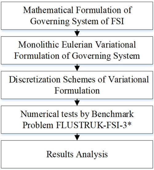
Figure 1.
Core steps in the study.
Contributions of the Study
Fluid–structure interaction problems play an important role in the daily routine of life. In such problems, the physical features of flow depending on structure displacement are analyzed. A rich literature exists on analyzing different physical features of flow in a classical framework, but the non-classical framework still requires attention from researchers for this analysis. This study focuses on the following key points:
- The analysis of different micro-structural characteristics of flow by employing a monolithic Eulerian formulation to FSI problems of finite deformation by taking into account the Cosserat continuum in a non-classical framework.
- The use of a well-known classical benchmark test FLUSTRUK- FSI-3* in numerical tests for validation of the results in a non-classical framework.
- The implementation of algorithmic description with FreeFem ++.
The rest of the paper is organized as follows:
In Section 2, we detail the mathematical formulation of the present CFSI problem, where we introduce the basic notations used for the continuum description followed by the complete derivation of the governing equations of fluid and solid structures from conservation laws by employing constitutive equations in a monolithic Eulerian frame. In Section 3, we present the variational formulation of the CFSI model. Subsequently, in Section 4, based on the variational formulation, time and space discretization using a semi-implicit scheme and the finite element method are presented. Numerical tests and the comparative results from simulations are discussed and analyzed in Section 5 and Section 6. Finally, in Section 7, we draw conclusion with some future developments.
2. Mathematical Formulation from the General Laws of Continuum Mechanics
In this section, we detail the mathematical formulation of the present CFSI problem. We introduce the notations used for the continuum description of the FSI problem and the respective domains of fluid and structure models with boundary conditions. A complete derivation of the governing equations of fluid and solid structures from conservation laws by employing constitutive equations in a monolithic Eulerian frame is presented.
2.1. Fluid–Structure Interaction Description: Notations
Let be a time-dependent computational domain made of a fluid region and a solid region with no overlap: at any time The interface of fluid and structure is denoted by and the boundary of is Initially, and are prescribed. The part of on which either structure is clamped or fluid has a ‘no-slip condition’ is denoted by assumed to be independent of time. A geometrical representation of this description is shown in Figure 2 below.
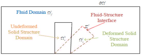
Figure 2.
Geometrical representation of the fluid–structure interaction description.
Based on standard notations in [1,19,47,48,49,50,51], we consider the Lagrangian position at time of or 3. The displacement, velocity, and micro-rotation fields are represented by and respectively. The transposed gradient and the Jacobian of the deformation are given as .
The density and the stress tensor at a given position and time are represented as and . In the case of an incompressible medium, the density remains constant for all time Denoting the density constants by and at any point and time we define density by using the set function indicator as
where
Similarly, the stress tensor is defined as
In this mathematical formulation, all spatial derivatives are taken with respect to and not with respect to If is a function of where then
Further, the deformation gradient and displacement field can be seen as a function of instead of In the case when is one-to-one and invertible, and are related mathematically as
and time derivatives are related by
Finally, we introduce the deformation tensor Du and the micro-rotation strain tensor as
A list of the notations used in the entire text is given below in Table 1.

Table 1.
List of the notations.
2.2. Conservation Laws
In a monolithic Eulerian frame, conservation of mass, conservation of linear momentum, and conservation of angular momentum for fluid and solid mediums take the form
The body force density, the body couple density, and the micro-inertia coefficient are denoted by , , and , respectively. Moreover, an incompressibility condition implies that and
2.3. Constitutive Equations
We consider a two-dimensional hyper-elastic incompressible Mooney–Rivlin material and an incompressible viscous Cosserat fluid.
- For a hyper-elastic incompressible material, the constitutive equation is
The Helmholtz potential for a Mooney–Rivlin material is given by
where constants and are empirically determined [51].
Consequently,
Taking and applying the Cayley–Hamilton theorem Equation (14) leads to
where is some scalar function of material constants and .
- For an incompressible viscous Cosserat fluid, the constitutive equations are described as
2.4. The Governing Equations of Cosserat Fluid in a Non-Classical Framework
Subjected to certain prescribed boundary conditions according to the description of the physical problem and taking into consideration the constitutive Equations (16) and (17), the governing conservation Equations (9)–(11) for an incompressible viscous Cosserat fluid as described in [39] leads to
where and are material parameters related to micro-viscosities.
In the above governing system, the conservation of linear momentum becomes independent of the micro-rotation in case of = 0. The governing system reduces to the classical Navier–Stokes system if the coefficients of micro-viscosity and the body couple density vanish.
3. Monolithic Eulerian Variational Formulation in 2D
In this non-classical variational formulation, homogeneous boundary conditions on are considered, i.e., either a solid is clamped or a fluid has a ‘no-slip condition’ and homogeneous Neumann conditions on For an incompressible material, the Cosserat fluid–structure interaction CFSI formulation in two dimensions thus reads:
Given , and , at , find with and , such that
taking and , where and are defined incrementally by and
The relation in defines and forward in time, while the notations and are used.
4. Discretization Schemes for a Monolithic Eulerian Variational Formulation
In this section, we propose the discretization schemes in time and space of the present non-classical CFSI problem based on its variational Formulations (21) and (22). The study employs a semi-implicit scheme and the finite element method to discretize respective domains.
4.1. Time Discretization Scheme
Let be the time of simulation where is the total time. The interval is discretized into equal subintervals each of the length such that where Let Hence
Now, if is a first-order approximation of defined by where such that then a first-order-in-time approximation for the CFSI problem of Equations (21) and (22) reads:
Find and such that with and with and the following holds
Now, update by and by where
4.2. Space Discretization Scheme
Let and represent the finite element functional spaces for the velocities, displacements, and micro-rotational velocities, respectively, and let be the functional space for the pressure field. Let be a triangulation of the initial domain with quadratic elements for displacements and translational and micro-rotational velocities, and linear elements for the pressure field. Given that the pressure is different in the fluid domain and structural domain because of the discontinuity of pressure at the fluid–structure interface , the functional space is the space of piecewise linear functions on the triangulation and is continuous in . A small penalization parameter needs to be added to impose the uniqueness of the pressure when one desires to use a direct linear solver. The discrete variational formulation of CFSI thus reads:
Find with and are subspaces of and such that
To update the triangulation at each vertex (say ) of the triangle the vertex is moved to a new position by
By denoting it can be seen that
This implies that the displacement vector of vertices can be copied to plus the addition of in order to obtain i.e.,
Moreover, the fluid domain mesh is moved by which is a solution of the Laplace problem subjected to where is the Cosserat fluid–structure interface and at the boundaries Moving the vertices of each triangle by the above procedure gives a new triangulation
5. Numerical Tests in a Non-Classical Framework
In this section, the numerical results for the present non-classical FSI problem are obtained by computing FLUSTRUK-FSI-3*, which is an incompressible variant of the successful classical FSI benchmark test problem FLUSTRUK-FSI-3. The spatial discretization is performed by using Lagrangian triangular finite elements with quadratic elements for displacements and translational and micro-rotational velocities, and linear elements for the pressure field. The publicly available tool FreeFem++ [42] has been used to implement the algorithms.
5.1. The Cylinder–Flag Test
The selection of this prominent classical FSI benchmark test FLUSTRUK-FSI-3* ‘flow around a cylinder’, is based on its complexity and implementation which has remained challenging, especially in a non-classical framework. Moreover, this test is most relevant to the proposed FSI problem and is reliable for achieving the desired accuracy in results for analyzing the micro-structural characteristics of flow in a non-classical framework. The results are then compared and validated with the classical solutions present in the literature [9,12,41].
This benchmark test problem was first studied by [40] and later by [9,12,41]. The description of the model problem under consideration is shown schematically in Figure 3. For numerical tests, a hyper-elastic incompressible Mooney–Rivlin material, like a rectangular flag of size is attached at the back of a hard, fixed cylinder in the computational rectangular domain ; the fluid flow enters and leaves freely at the left inlet and the right outlet.
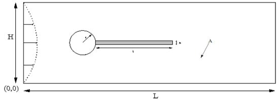
Figure 3.
Computational domain of the model problem.
5.2. Geometry, Boundary, and Initial Conditions
We consider the geometry, boundary conditions, and initial conditions for the flag–cylinder test described in [9] as:
Geometry: the point (0.2 m, 0.2 m)) and = 0.05 m are center and radius of a cylinder; other parameters are considered in the computation as = 0.35 m, = 0.02 m, = 2.5 m, and = 0.41 m, which puts the cylinder slightly below the symmetry line of the computational domain.
Boundary and initial conditions: top and bottom boundaries satisfy the ‘no-slip’ condition. A parabolic velocity profile is prescribed at the left inlet, where is mean inflow velocity with flux and = 2. The zero-stress is employed at the right outlet using the ‘do-nothing’ approach. Initially, all velocities and structure displacements are zero.
In addition, the density and the reduced kinematic viscosity of the fluid takes values = 103 kgm−3 and = 10−3 m2s−1. For a solid structure, we consider = 106 kgm−1s−1 and no external force.
6. Results Analysis
In this section, the results obtained are utilized to analyze some interesting micro-structural characteristics of flow in a non-classical CFSI problem. In this regard, we find the relationship between the amplitude of oscillations and the material parameters and by validating the results with classical benchmark solutions followed by determining the effects of micro-rotational viscosity on the velocity and the micro-rotation fields. During numerical simulation, the flow starts oscillating and develops a Karman vortex street around . Figure 4 and Figure 5 show the horizontal and vertical displacement of the flagella end tip by using micro-viscosity and micro-inertia parameters, respectively. The results are obtained with a mesh of 2199 vertices and a uniform time step size of 0.005 s. The frequency 4.5 s−1 and the amplitude 0.03 are found to be the same as in [9], which validates the results of the present non-classical model with classical benchmark solutions. Here, and denote the coefficient of micro-inertia and micro-rotational viscosity, respectively, while combines the shear spin and rotational spin viscosities in the numerical simulation.
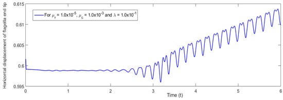
Figure 4.
Horizontal displacement of flagella end tip against time in a non-classical framework shown up to t = 6.
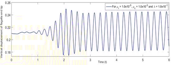
Figure 5.
Vertical displacement of flagella end tip against time in a non-classical framework shown up to t = 6.
The structural and fluid parameters c = c1 and play important roles in the numerical simulation and have a significant effect on the vertical displacement of the flagella end tip. The results suggest that the amplitude of oscillations varies inversely with the material parameters c1 and as displayed in Figure 6 and Figure 7, respectively. Further, the amplitude of oscillations becomes stable relatively more quickly by increasing c1 than increasing , which leads to the almost vanishing of the oscillations and makes c1 very sensitive.
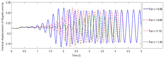
Figure 6.
Vertical displacement of flagella end tip against in a non-classical framework shown up to t = 5.
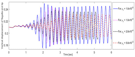
Figure 7.
Vertical displacement of flagella end tip against in a non-classical framework shown up to t = 6.
After validation, the effects of the micro-rotational viscosity on the velocity and micro-rotation fields were analyzed to understand the micro-structural characteristics of flow by comparing the results with the classical case of FSI solutions. The results in Figure 8 indicate that the increase in micro-rotational viscosity causes significantly larger micro-rotations in flow at the micro-structural level. This micro-rotational effect vanishes in the classical case which strengthen the governing dynamics of the Cosserat continuum for the present coupling problem in a non-classical framework.
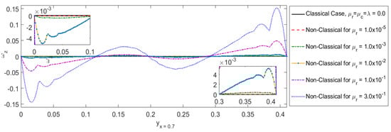
Figure 8.
Effects of micro-rotational viscosity on the micro-rotation field by comparing the results with classical solution.
Despite producing large micro-rotation, it is observed that micro-rotational viscosity does not affect the velocity profiles of flow as shown in Figure 9 and Figure 10. The magnitude of the horizontal velocity of fluid particles is found to be somewhat greater than that of the vertical velocity against a large value of in the computational domain. All the numerical results are obtained by taking the Reynolds number and mean velocity and the relation between them is found to be linear.
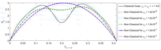
Figure 9.
Effects of micro-rotational viscosity on horizontal velocity profile of flow by comparing the results with classical solution.
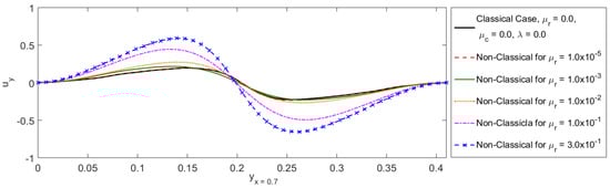
Figure 10.
Effects of micro-rotational viscosity on vertical velocity profile of flow by comparing the results with classical solution.
Finally, in Figure 11, some color snapshots are presented to show the velocity profile and behavior of the flagella pictorially in FSI phenomena at different times during the numerical simulation. In these color snapshots, the displacement of the solid structure can be seen clearly during the simulation which in turn affects the flow domain and produces Karman vortices. (Note: we only represent the most significant and visible color legend to show the velocity magnitudes in the fluid flow simulation.)
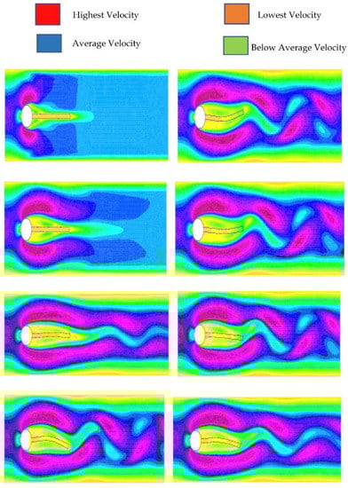
Figure 11.
Velocity profile (column 1: t = 0.1, 0.3, 1.95, 2.3, and column 2: t = 2.44, 2.46, 2.48, 2.52).
7. Conclusions
In this paper, a monolithic Eulerian formulation has been presented for fluid–structure interaction (FSI) problems with large structural displacements in a non-classical framework to study the micro-structural characteristics of fluid flow by validating the results with classical benchmark solutions. In this respect, the Cosserat theory of continuum taking into account the micro-rotational degrees of freedom of the particles has been considered. The mathematical formulation of the governing system has been derived from the general laws of continuum mechanics. The finite element method and semi-implicit scheme were proposed to discretize space and time domains, respectively. The results of the study were obtained by a well-known classical FSI benchmark test problem FLUSTRUK-FSI-3* with FreeFem++. The results of the study indicated that the effect of increasing the micro-rotational viscosity on the micro-rotation field was significantly large compared to the velocity field in fluid flow at the micro-structural level. It has also been observed that the amplitude of oscillations was related inversely to the material parameters c1 and while increasing c1 stabilized the amplitude of oscillations relatively more quickly than increasing in the computer simulations. Furthermore, the micro-rotational effect vanished in the classical framework which strengthened the governing dynamics of the present FSI model in a non-classical framework. Finally, the present study can be extended to analyze the effect of other micro-viscosity parameters on velocity fields in FSI phenomena with an additional benchmark test using significant computational resources for better results in a non-classical framework.
Author Contributions
Conceptualization, N.H.H.; Data curation, N.H.H.; Formal analysis, M.S.K. and L.L.; Investigation, L.L.; Methodology, N.H.H. and L.L.; Project administration, M.S.K.; Resources, N.H.H.; Software, M.S.K.; Supervision, L.L. All authors have read and agreed to the published version of the manuscript.
Funding
This research is funded by the Department of Engineering Structure and Mechanics, Wuhan University of Technology, Wuhan, China.
Institutional Review Board Statement
Not applicable.
Informed Consent Statement
Not applicable.
Data Availability Statement
Some preliminary inconclusive results of the present study can be seen at https://arxiv.org/abs/2204.03530 and https://arxiv.org/abs/2203.16493 (accessed on 13 March 2022).
Acknowledgments
Thanks to Mumtaz Ali Kaloi for his unconditional technical support.
Conflicts of Interest
The authors declare no conflict of interest regarding this research paper.
References
- Hron, J.; Turek, S. A monolithic FEM solver for an ALE formulation of fluid-structure interaction with configuration for numerical benchmarking. In ECCOMAS CFD 2006: Proceedings of the European Conference on Computational Fluid Dynamics, Egmond aan Zee, The Netherlands, 5–8 September 2006.
- Dunne, T. An Eulerian approach to fluid–structure interaction and goal-oriented mesh adaptation. Int. J. Numer. Methods Fluids 2006, 51, 1017–1039. [Google Scholar] [CrossRef]
- Heil, M.; Hazel, A.L.; Boyle, J. Solvers for large-displacement fluid–structure interaction problems: Segregated versus monolithic approaches. Comput. Mech. 2008, 43, 91–101. [Google Scholar] [CrossRef]
- Wang, Y.; Jimack, P.K.; Walkley, M.A.; Pironneau, O. An energy stable one-field monolithic arbitrary Lagrangian–Eulerian formulation for fluid–structure interaction. J. Fluids Struct. 2020, 98, 103117. [Google Scholar] [CrossRef]
- Murea, C.M. Three-Dimensional Simulation of Fluid–Structure Interaction Problems Using Monolithic Semi-Implicit Algorithm. Fluids 2019, 4, 94. [Google Scholar] [CrossRef]
- Schott, B.; Ager, C.; Wall, W.A. A monolithic approach to fluid-structure interaction based on a hybrid Eulerian-ALE fluid domain decomposition involving cut elements. Int. J. Numer. Methods Eng. 2019, 119, 208–237. [Google Scholar] [CrossRef]
- Pironneau, O. An energy stable monolithic Eulerian fluid-structure numerical scheme. Chin. Ann. Math. Ser. B 2018, 39, 213–232. [Google Scholar] [CrossRef]
- Sauer, R.A.; Luginsland, T. A monolithic fluid–structure interaction formulation for solid and liquid membranes including free-surface contact. Comput. Methods Appl. Mech. Eng. 2018, 341, 1–31. [Google Scholar] [CrossRef]
- Hecht, F.; Pironneau, O. An energy stable monolithic Eulerian fluid-structure finite element method. Int. J. Numer. Methods Fluids 2017, 85, 430–446. [Google Scholar] [CrossRef]
- Chiang, C.-Y.; Pironneau, O.; Sheu, T.W.H.; Thiriet, M. Numerical study of a 3D Eulerian monolithic formulation for incompressible fluid-structures systems. Fluids 2017, 2, 34. [Google Scholar] [CrossRef]
- Pironneau, O. Numerical study of a monolithic fluid–structure formulation. In Variational Analysis and Aerospace Engineering; Springer: Cham, Switzerland, 2016; pp. 401–420. [Google Scholar]
- Dunne, T.; Rannacher, R. Adaptive finite element approximation of fluid-structure interaction based on an Eulerian variational formulation. In Fluid-Structure Interaction; Springer: Berlin/Heidelberg, Germany, 2006; pp. 110–145. [Google Scholar]
- Richter, T.; Wick, T. Finite elements for fluid–structure interaction in ALE and fully Eulerian coordinates. Comput. Methods Appl. Mech. Eng. 2010, 199, 2633–2642. [Google Scholar] [CrossRef]
- Rannacher, R.; Richter, T. An adaptive finite element method for fluid-structure interaction problems based on a fully eulerian formulation. In Fluid Structure Interaction II; Springer: Berlin/Heidelberg, Germany, 2011; pp. 159–191. [Google Scholar]
- Richter, T. A fully Eulerian formulation for fluid–structure-interaction problems. J. Comput. Phys. 2013, 233, 227–240. [Google Scholar] [CrossRef]
- Wick, T. Fully Eulerian fluid–structure interaction for time-dependent problems. Comput. Methods Appl. Mech. Eng. 2013, 255, 14–26. [Google Scholar] [CrossRef]
- Formaggia, L.; Gerbeau, J.; Nobile, F.; Quarteroni, A. On the coupling of 3D and 1D Navier–Stokes equations for flow problems in compliant vessels. Comput. Methods Appl. Mech. Eng. 2001, 191, 561–582. [Google Scholar] [CrossRef]
- Nobile, F. Numerical Approximation of Fluid-Structure Interaction Problems with Application to Haemodynamics (No. THESIS); EPFL: Milan, Italy, 2001. [Google Scholar]
- Le Tallec, P.; Mouro, J. Fluid structure interaction with large structural displacements. Comput. Methods Appl. Mech. Eng. 2001, 190, 3039–3067. [Google Scholar] [CrossRef]
- Gerbeau, J.F.; Vidrascu, M. A quasi-Newton algorithm based on a reduced model for fluid-structure interaction problems in blood flows. ESAIM Math. Model. Numer. Anal. 2003, 37, 631–647. [Google Scholar] [CrossRef]
- Fernández, M.A.; Moubachir, M. A Newton method using exact Jacobians for solving fluid–structure coupling. Comput. Struct. 2005, 83, 127–142. [Google Scholar] [CrossRef]
- Dettmer, W.; Perić, D. A computational framework for fluid–structure interaction: Finite element formulation and applications. Comput. Methods Appl. Mech. Eng. 2006, 195, 5754–5779. [Google Scholar] [CrossRef]
- Murea, C.M. Numerical simulation of a pulsatile flow through a flexible channel. ESAIM Math. Model. Numer. Anal. 2006, 40, 1101–1125. [Google Scholar] [CrossRef]
- Mbaye, I.; Murea, C.M. Numerical procedure with analytic derivative for unsteady fluid–structure interaction. Commun. Numer. Methods Eng. 2008, 24, 1257–1275. [Google Scholar] [CrossRef]
- Kuberry, P.; Lee, H. A decoupling algorithm for fluid-structure interaction problems based on optimization. Comput. Methods Appl. Mech. Eng. 2013, 267, 594–605. [Google Scholar] [CrossRef]
- Donea, J. Arbitrary Lagrangian-Eulerian finite element analysis. Comput. Methods Transient Anal. 1983, 474–516. [Google Scholar]
- Quarteroni, A.; Formaggia, L. Mathematical modelling and numerical simulation of the cardiovascular system. Handb. Numer. Anal. 2004, 12, 3–127. [Google Scholar]
- Nobile, F.; Vergara, C. An effective fluid-structure interaction formulation for vascular dynamics by generalized Robin conditions. SIAM J. Sci. Comput. 2008, 30, 731–763. [Google Scholar] [CrossRef]
- Formaggia, L.; Quarteroni, A.; Veneziani, A. Cardiovascular Mathematics, Volume 1 of MS&A. Modeling, Simulation and Applications; Springer: Berlin/Heidelberg, Germany, 2009. [Google Scholar]
- Le Tallec, P.; Hauret, P. Energy conservation in fluid structure interactions. In Numerical Methods for Scientific Computing. Variational Problems and Applications; Neittanmaki, P., Kuznetsov, Y., Pironneau, O., Eds.; CIMNE: Barcelona, Spain, 2003. [Google Scholar]
- Basting, S.; Quaini, A.; Čanić, S.; Glowinski, R. Extended ALE method for fluid–structure interaction problems with large structural displacements. J. Comput. Phys. 2017, 331, 312–336. [Google Scholar] [CrossRef]
- Liu, J. A second-order changing-connectivity ALE scheme and its application to FSI with large convection of fluids and near contact of structures. J. Comput. Phys. 2016, 304, 380–423. [Google Scholar] [CrossRef]
- Peskin, C.S. The immersed boundary method. Acta Numer. 2002, 11, 479–517. [Google Scholar] [CrossRef]
- Wang, Y.; Jimack, P.K.; Walkley, M.A. A one-field monolithic fictitious domain method for fluid–structure interactions. Comput. Methods Appl. Mech. Eng. 2017, 317, 1146–1168. [Google Scholar] [CrossRef]
- Cosserat, E.; Cosserat, F. Theorie des Corps Déformables; Hermann: Paris, France, 1909. [Google Scholar]
- Eringen, A.C. Theory of micropolar fluids. J. Math. Mech. 1966, 16, 1–18. [Google Scholar] [CrossRef]
- Eringen, A.C. Simple microfluids. Int. J. Eng. Sci. 1964, 2, 205–217. [Google Scholar] [CrossRef]
- Condiff, D.; Dahler, W.J.S. Fluid mechanical aspects of antisymmetric stress. Phys. Fluids 1934, 7, 842–854. [Google Scholar] [CrossRef]
- Lukaszewicz, G. Micropolar Fluids: Theory and Applications; Springer Science & Business Media: Berlin/Heidelberg, Germany, 1999. [Google Scholar]
- Schafer, M.; Turek, S. Benchmark computations of laminar flow around a cylinder. Notes Numer. Fluid Mech. 1996, 52, 547–566. [Google Scholar]
- Turek, S.; Hron, J. Proposal for numerical benchmarking of fluid-structure interaction between an elastic object and laminar incompressible flow. In Fluid-Structure Interaction; Springer: Berlin/Heidelberg, Germany, 2006; pp. 371–385. [Google Scholar]
- Hecht, F. New development in FreeFem++. J. Numer. Math. 2012, 20, 251–266. [Google Scholar] [CrossRef]
- Kim, C.; Jung, M.; Yamada, T.; Nishiwaki, S.; Yoo, J. Freefem++ code for reaction-diffusion equation–based topology optimization: For high-resolution boundary representation using adaptive mesh refinement. Struct. Multidiscip. Optim. 2020, 62, 439–455. [Google Scholar] [CrossRef]
- Dapogny, C.; Frey, P.; Omnès, F.; Privat, Y. Geometrical shape optimization in fluid mechanics using FreeFem++. Struct. Multidiscip. Optim. 2018, 58, 2761–2788. [Google Scholar] [CrossRef]
- Krivovichev, G.V. A computational approach to the modeling of the glaciation of sea offshore gas pipeline. Int. J. Heat Mass Transf. 2017, 115, 1132–1148. [Google Scholar] [CrossRef]
- Danaila, I.; Moglan, R.; Hecht, F.; Le Masson, S. A Newton method with adaptive finite elements for solving phase-change problems with natural convection. J. Comput. Phys. 2014, 274, 826–840. [Google Scholar] [CrossRef]
- Belytschko, T.; Liu, W.K.; Moran, B.; Elkhodary, K. Nonlinear Finite Elements for Continua and Structures; John Wiley & Sons: Hoboken, NJ, USA, 2014. [Google Scholar]
- Batra, R.C. Elements of Continuum Mechanics; AIAA: Reston, Virginia, USA, 2006. [Google Scholar]
- Bath, K.J. Finite Element Procedures; Englewood Cliffs: Prentice-Hall, NJ, USA, 1996. [Google Scholar]
- Marsden, J.T.; Hughes, J.R. Mathematical Foundations of Elasticity; Dover Publications: New York, NY, USA, 1993. [Google Scholar]
- Ciarlet, P.G. Mathematical Elasticity: Volume I: Three-Dimensional Elasticity; Elsevier: Amsterdam, The Netherlands, 1988. [Google Scholar]
Publisher’s Note: MDPI stays neutral with regard to jurisdictional claims in published maps and institutional affiliations. |
© 2022 by the authors. Licensee MDPI, Basel, Switzerland. This article is an open access article distributed under the terms and conditions of the Creative Commons Attribution (CC BY) license (https://creativecommons.org/licenses/by/4.0/).