Binned Term Count: An Alternative to Term Frequency for Text Categorization

Abstract

In text categorization, a well-known problem related to document length is that larger term counts in longer documents cause classification algorithms to become biased. The effect of document length can be eliminated by normalizing term counts, thus reducing the bias towards longer documents. This gives us term frequency (TF), which in conjunction with inverse document frequency (IDF) became the most commonly used term weighting scheme to capture the importance of a term in a document and corpus. However, normalization may cause term frequency of a term in a related document to become equal or smaller than its term frequency in an unrelated document, thus perturbing a term’s strength from its true worth. In this paper, we solve this problem by introducing a non-linear mapping of term frequency. This alternative to TF is called binned term count (BTC). The newly proposed term frequency factor trims large term counts before normalization, thus moderating the normalization effect on large documents. To investigate the effectiveness of BTC, we compare it against the original TF and its more recently proposed alternative named modified term frequency (MTF). In our experiments, each of these term frequency factors (BTC, TF, and MTF) is combined with four well-known collection frequency factors (IDF), RF, IGM, and MONO and the performance of each of the resulting term weighting schemes is evaluated on three standard datasets (Reuters (R8-21578), 20-Newsgroups, and WebKB) using support vector machines and K-nearest neighbor classifiers. To determine whether BTC is statistically better than TF and MTF, we have applied the paired two-sided t-test on the macro $F_1$ results. Overall, BTC is found to be 52% statistically significant than TF and MTF. Furthermore, the highest macro $F_1$ value on the three datasets was achieved by BTC-based term weighting schemes.

1. Introduction

Text classification is considered one of the most significant research domains in data mining and machine learning. The main goal of text classification is to automatically arrange documents into various known categories, also known as classes [1,2,3]. Due to the nature of text documents, text classification faces several challenges, such as the numerical representation of documents, high dimensionality, and high skew of classes [4]. Our work mainly focuses on the numerical representation of words in documents.

Choosing an appropriate representation for words (terms and words are used interchangeably throughout this text) present in a collection of documents, which is called a corpus, is crucial to obtain good classification performance [5]. Different representations have been proposed in the literature to maximize the accuracy of machine learning algorithms. For example, N-grams [6], individual words (uni-grams) [3], multi-words or phrases (capturing contextual information of individual words) [7] have been used. Among these models, the most widely used is bag-of-words (BoW) [8] representation. This representation describes the occurrences of words within a document. A document can be represented in a vector form as $d_j=<w_{1j},w_{2j},w_{3j},...,w_{Nj}>$, where $w_{ij}$ is the term weight of the ith term (denoted by $t_i$) in document j and N is the total number of terms in the corpus [9]. N-grams, uni-grams, and BoW can also be used interchangeably, as these terms refer to the same representation when N = 1 in the N-grams. Nevertheless, if N = 2 is in N-grams, then two adjoining words will be referred to as a single term. The weight of a term indicates its importance in a document and the corpus. As an example, the number of occurrences of a term in a document can be used as its weight. This is called term count ($tc$) and captures document-specific worth of a term [10]. The drawback of using the BoW approach is that it removes all semantic and syntactic information as it ignores the position of terms. BoW loses grammatical structure, tone, and other elements of a sentence and provides occurrence information of terms. However, it is simple and performs well for the text categorization tasks [11,12].

Having selected the model, the next step is to represent the terms numerically [7]. A term weighting scheme (or feature representation method) generates the term weights. In this regard, the researchers of text classification have borrowed the design concepts from the information retrieval domain. There are three factors considered in assigning weights to terms [13]. First is the term frequency factor, which closely represents the document’s content and is based on term occurrences in a document. The second factor is called the collection frequency factor. It can discriminate all the relevant documents from other irrelevant ones. The third is a normalization factor to equalize the length of the documents, thus taking the effect of document length into account. These three factors are combined to assign the weights of the terms, which are used to perform the following steps of text classification, such as preprocessing (e.g., pruning), feature selection, and classifier learning algorithm [10]. For example, it was found that the performance of the support vector machines (SVM) classifier depends primarily on feature representation rather than its kernel function [14,15]. Therefore, the primary goal in designing these three factors is to capture the true worth of a term so that its weight denotes how much it contributes to the categorization task of the document.

The most widely used term weighting scheme in text classification is term frequency and inverse document frequency (TF-IDF) [16,17]. The former is a term frequency factor, while the latter is a collection frequency factor. Researchers borrowed from the information retrieval domain have raised questions about its suitability in classifying texts. They have pointed out various issues related to TF as well as IDF. Towards this end, different research works have proposed new individual factors or term weighting schemes for the improvement of text classification performance [7,10,18]. Most of these works focus on proposing alternatives to IDF, and more work needs to be done to improve the performance of TF. One such variant of TF that was more recently proposed is modified term frequency (MTF) [19]. It directly modifies the raw term count using all training documents’ length information instead of the common normalization factor. In this paper, we found out that when the term counts of a term are normalized by document length to obtain term frequency, TF can change a term’s strength from its true worth. The MTF factor does the same. Their problems are illustrated with the help of a real-life dataset example. To address the problems, we propose an alternative to TF named binned term count (BTC), which gives a representation better than TF and MTF. To show the effectiveness of BTC against TF and MTF, we conduct experiments on three well-known datasets. These three-term frequency factors are combined with four collection frequency factors, and performances are evaluated with SVM and K-nearest neighbors (KNN) classifiers.

The remaining paper is organized as follows: Section 2 presents a survey of different feature representation techniques. In Section 3, we provide a rationale for the proposed feature representation factor BTC and explain its working. An experimental setup is described in Section 4, while results and their discussion are given in Section 5. The conclusions are drawn in Section 6.

2. Related Works

A term weighting scheme estimates the worth of terms in a document and corpus and assigns a score or weight to the terms accordingly. The importance of a term, based on how well it discriminates different classes, can be determined at (1) the document level and (2) the corpus level. The former is estimated by the number of occurrences of a term in a document, while the latter is calculated by the number of occurrences in a corpus. In a given document, a frequent term (a term occurring in many corpus documents) is more critical than a less frequent term. On the contrary, a commonplace term in documents of a corpus is considered to play a negative role in determining the document class [14,20]. A term found in almost all the classes will have poor discrimination power. Additionally, the length of documents may vary in a corpus. Longer documents usually have higher term counts and more terms than shorter documents. Thus, longer documents may produce higher similarity to user queries than shorter documents while retrieving documents [21,22]. Researchers have proposed different solutions based on these concepts, which can be divided into two broad categories.

This section is divided into three sub-sections. The Section 2.1 covers the term frequency factors present in the literature. The Section 2.2 is about collection frequency factors that are commonly used. At the same time, the Section 2.3 covers recent text representation techniques used in text classification.

2.1. Estimating Document Level Worth with a Term Frequency Factor

Salton and Buckley [13] proposed to normalize the term counts by the maximum term count in the same document. The term frequency of the ith term in the jth document, denoted by $T{F}_{(t_i,d_j)}$, is given by,

$$T{F}_{(t_i,d_j)}=\frac{t{c}_{ij}}{\underset{tc}{max}\left(d_j\right)}$$

(1)

where $t{c}_{ij}$ is the term count of the ith term and $\underset{tc}{max}\left(d_j\right)$ is the maximum term count in the jth document. As longer documents are expected to have larger term counts, values for $\underset{tc}{max}$ will be larger as compared to shorter documents.

The most commonly used normalization is to normalize term counts by the total number of words present in the document [23,24].

$$T{F}_{(t_i,d_j)}=\frac{t{c}_{ij}}{size\left(d_j\right)}$$

(2)

where $t{c}_{ij}$ is the term count of ith term in the document $d_j$ and $size\left(d_j\right)$ is sum of term counts of all terms in the document $d_j$. As longer documents mean larger values of $size\left(d_j\right)$, this normalization will lower the term frequencies in longer documents so that they are now comparable with term frequencies in shorter documents.

As described in [25], term frequency of a term strongly related to a class should be higher than that of an unrelated term in documents of that class. Term frequencies estimated in Equations (1) and (2) may not truly represent the importance of a term, because term frequency of terms strongly related to a class may become smaller than that of unrelated terms in documents of that class due to these normalizations. We illustrate this problem in Section 3.

Lan et al. [11] suggested the use of logarithm of term frequency to minimize effect of higher term frequencies. This normalization is given by,

$$T{F}_{(t_i,d_j)}=1+log\left(t{c}_{ij}\right)$$

(3)

where $T{F}_{(t_i,d_j)}$ is the term frequency and $t{c}_{ij}$ is the term count of the ith term.

In shorter documents, term counts will typically not attain larger values. Binary weights can be assigned to terms instead of using term counts. Forman [10] experimented on corpuses with small documents and, thus tested the concept of binary weights. Binary weights eliminate the effect of number of occurrences but do not produce good results when used for longer documents.

In [26], Sabbah et al., proposed modified term frequency (mTF). The main idea behind the proposed scheme is to include the proportion of the total number of term frequency in all collection’s documents to the total number of distinctive terms in the collection. The normalization is also applied by the fractional relation of length of document and number of distinctive terms in the collection. For the term i in the jth document is given by,

$$mT{F}_{(t_i,d_j)}=\frac{t{c}_{ij}\times log\left(\frac{T_i}{T_c}\right)}{log\left({\displaystyle \sum _{i=1}^n}t{c}_{ij}^2\times \frac{size{\left(d_j\right)}^2}{T_c}\right)}$$

(4)

where $T_i$ and $T_c$ denote the total number of the natural frequency of the ith terms in all documents in all collections and the total number of specific terms in the collection, respectively, by comparing mTF with TF, it was found to produce better results than document frequency (DF), TF-IDF, and TF-RF.

Documents in a corpus can be of variable lengths. Longer documents can have more effect in distinguishing the classes of documents. Therefore, normalization is performed to reduce the effect of the length of a document and is calculated by dividing the term frequency with the total number of terms. Chen et al. [19] found that information gets lost in the cosine normalization process. To solve this problem, they proposed a factor named modified term frequency (MTF) that considers the length information of all the training documents into the term frequency factor.

$$MT{F}_{(t_i,d_j)}=\sqrt{t{c}_{ij}\times {log}_2\left(1+\frac{avg\_size}{size\left(d_j\right)}\right)}$$

(5)

where $t{c}_{ij}$ indicates the raw term frequency of the ith term in document $d_j$. While $avg\_size$ indicates the average length of all training documents and $size\left(d_j\right)$ indicates the actual length of jth document.

2.2. Estimating Corpus Level Worth with a Collection Frequency Factor

Irrespective of term count, a term is considered to lose its discrimination power as it becomes more frequent in a corpus. Among classes, less frequent terms are considered more discriminant than frequent terms. Term frequency is a document-level measure to capture the importance of a term in a document. The term weight should also include how discriminating a term is in the whole corpus. Thus term frequency alone is not considered to be used as a term weight.

Inverse document frequency (IDF) is the most widely used collection frequency factor to estimate the importance of a term in the corpus. It assigns smaller values to frequent words and higher values to less frequent words. IDF for the ith term is given by [25,27],

$$ID{F}_{\left(t_i\right)}=\frac{logD}{{df}_i}$$

(6)

where D is the total number of documents in the corpus and ${df}_i$ is the number of documents containing the ith term, and is called document frequency [28,29]. TF favors long documents, while IDF is biased towards documents belonging to rare categories. In a dataset, representative terms for a category happen to occur mostly in their respective categories. In skewed datasets, terms belonging to those categories with many documents will suffer because their IDF value will be low and vice versa. This is because the frequent occurrence of a term across many documents decreases its IDF. A combination of term frequency and inverse document frequency, called TF-IDF, is commonly used to represent term weight [16,30]. For the ith term, it is given by,

$$TF-ID{F}_{(t_i,d_j)}=T{F}_{(t_i,d_j)}\times ID{F}_{\left(t_i\right)}$$

(7)

Due to the supervised nature of text classification, a number of term weighting schemes have been proposed that use the class label information while calculating the term weight. Some related works are given next.

Debole and Sebastiani introduced supervised term weighting schemes for the first time by combining CHI-square, gain ratio (GR), and information gain (IG) with TF and compared their results with standard TF-IDF [31]. They proposed TF-CHI, TF-GR, and TF-IG and emphasized that feature selection-based term weighting schemes are likely to perform better than traditional text classification.

In [32], inverse class frequency (ICF) was proposed, basically a supervised term weighting scheme. Instead of using the document frequency of a term, it takes into account the number of categories in which a term appears. For the ith term, ICF is calculated as given by,

$$IC{F}_{\left(t_i\right)}=log\frac{\left|C\right|}{cf\left(t_i\right)}$$

(8)

where $\left|C\right|$ is the total number of classes while $cf\left(t_i\right)=|c:t_i\in c|$ is number of classes in which the term $t_i$ appears. ICF considers that if a term occurs in a few classes, then it strongly belongs to those classes, thus assigning higher weights to infrequent terms. Based on this behaviour of ICF, Wang and Zhang [33] introduced the combination of ICF with TF, which is given by,

$$TF-IC{F}_{(t_i,d_j)}=T{F}_{(t_i,d_j)}\times log\frac{\left|C\right|}{cf\left(t_i\right)}$$

(9)

The number of classes within a corpus is minimal, and the chances are high that a term may occur in multiple classes or sometimes in all classes [20,34]. Thus ICF fails to assign appropriate weights in some instances. To overcome these problems, Ren et al., introduced novel term weighting schemes by using the idea of ICF [35]. TF-IDF-ICF was used to weigh the terms so that the term distinguishing power among documents and classes could be considered. Furthermore, a new factor was introduced called inverse class space density frequency (ICSDF) to consider that a term may appear in any other class as a false positive.

Lan et al., proposed a new supervised weight factor named relevance frequency (RF) in [36]. It considers the distribution of a term in different categories. A term more concentrated in the positive class than the negative class is considered to have stronger discrimination power. It is calculated as:

$$R{F}_{\left(t_i\right)}=log\left(2+\frac{t{p}_i}{max(1,f{p}_i)}\right)$$

(10)

where $t{p}_i$ denotes the number of documents in the positive category that contain term $t_i$ and $f{p}_i$ is the number of documents in the negative category that contain this term. According to [37], TF-RF might not be an optimal solution as it groups the multiple classes into single negative class and ignores precise distribution of a term across multiple classes of document.

Wang and Zhang [33] combined both $RF$ and $ICF$ into a new weighting scheme called $ICF-based$. For ith term and jth document, it is given as

$$ICF-base{d}_{(t_i,d_j)}=T{F}_{(t_i,d_j)}\times log\left(2+\frac{t{p}_i}{max(1,f{p}_i)}\times \frac{\left|C\right|}{cf\left(t_i\right)}\right)$$

(11)

Another collection frequency factor is the inverse gravity measure (IGM), which measures the inter-class distribution concentration of a term. It considers a term concentrated in one class more important than a term having relatively uniform distribution on several classes or all classes [37]. The more scattered a term is in different classes, the lesser will be its IGM value. The IGM weight of a term $t_i$ is calculated as:

$$IG{M}_{\left(t_i\right)}=\frac{1}{{\displaystyle \sum _{j=1}^{\left|C\right|}}\frac{f_{ij}}{{\displaystyle \underset{1\le k\le \left|C\right|}{max}}\left(f_{ik}\right)}.j}$$

(12)

where $f_{ij}$ is class dependent document frequency $DF$ of a term $t_i$ in jth class, and ${\displaystyle \underset{1\le k\le \left|C\right|}{max}}\left(f_{ik}\right)$ is the maximum class dependent document frequency of the term $t_i$. In [38], it was observed that TF-IGM did not work well in three extreme cases. They proposed $TF-IG{M}_{max}$ by improving the collection frequency factor (IGM) performance and focusing on failure scenarios without affecting the previous performance.

Sabbah et al. [20] proposed to include short terms in the weighting process and presented new weighting schemes, namely mTF, mTFIDF, mTFmIDF, TFmIDF by suggesting changes in the conventional TF-IDF scheme. They found that text classification performance improves with mTFmIDF, mTFIDF, and mTF compared to the conventional term weighting techniques TF, TF-IDF, and Entropy when evaluated by SVM, KNN, Naïve Bayes classifiers on three well-known datasets.

Dogan et al., presented two novels that supervised term weighting techniques, namely TF-MONO and SRTF-MONO [39]. Besides using term occurrences in a specific class, they used non-occurrence information in the rest of the classes. The local MONO weight of term $t_i$ is given by,

$$\begin{array}{c}\hfill MON{O}_{{local}_{\left(t_i\right)}}=\frac{D_{{t_i}_{\_max}}}{D_{total}\left({t_i}_{\_max}\right)}\times \frac{D_{\overline{t_i}}}{D_{total}\left(\overline{t_i}\right)}\end{array}$$

(13)

The first factor is $M{O}_{\left(t_i\right)}$ and represents the ratio between the number of text documents in the class where $t_i$ occurs most and the total quantity of text documents in the corresponding class. The second factor is $N{O}_{\left(t_i\right)}$ and represents the ratio between the number of text documents in the rest of the classes where $t_i$ does not occur and the total quantity of text documents in the rest of the classes.

The global MONO weight of term $t_i$ is calculated as following:

$$MON{O}_{{global}_{\left(t_i\right)}}=1+\alpha \times MON{O}_{{local}_{\left(t_i\right)}}$$

(14)

$$TF-MON{O}_{(t_i,d_j)}=T{F}_{(t_i,d_j)}\times MON{O}_{{global}_{\left(t_i\right)}}$$

(15)

The authors have compared TF-MONO with five state-of-the-art term weighting techniques namely, TF-IDF-ICF, TF-IDF-ICSDF, TF-IDF, TF-RF, and TF-IGM, using machine learning algorithms, namely, SVM and KNN on three benchmark datasets Reuters-21578, WebKB, and 20-Newsgroups. TF-MONO and SRTF-MONO have shown better results as compared to conventional term weighting techniques. The frequently used term weighting schemes in the related work are presented in Table 1.

Table 1. Summary: Most commonly used term weighting schemes in literature.

(a) Term Frequency Factors
Factor Name	Weighting Formula	Description
TF [13]	$\frac{t{c}_{ij}}{\underset{tc}{max}\left(d_j\right)}$	Obtained by dividing term count and maximum term count
TF [23,24]	$\frac{t{c}_{ij}}{size\left(d_j\right)}$	Obtained by dividing term count and size of the documnet
TF [11]	$1+log\left(t{c}_{ij}\right)$	Obtained by taking the logarithm of term count
mTF  [26]	$\frac{t{c}_{ij}\times log\left(\frac{{\sqrt{T}}_c}{T_i}\right)}{log\left({\displaystyle \sum _{i=1}^n}t{c}_{ij}^2\times \frac{size{\left(d_j\right)}^2}{{\sqrt{T}}_c}\right)}$	Also uses the missing terms count information to calculate term count
MTF  [19]	$\sqrt{t{c}_{ij}\times {log}_2\left(1+\frac{avg\_size}{size\left(d_j\right)}\right)}$	Uses the average size of documents in the corpus to calculate term weight
(b) Collection Frequency Factors
IDF [25,27]	$\frac{logD}{{df}_i}$	Assigns smaller weights to the frequent terms and vice versa
ICF  [32]	$log\frac{\left|C\right|}{cf\left(t_i\right)}$	Considers Class frequency by replacing document frequency in IDF
RF  [36]	$log\left(2+\frac{t{p}_i}{max(1,f{p}_i)}\right)$	Considers distribution of a term across different categories and assigns
ICF-based RF  [33]	$log(2+\frac{t{p}_i}{max(1,f{p}_i)}\times \frac{\left|C\right|}{cf\left(t_i\right)}$	Combination of RF and ICF
IGM  [37]	$\frac{1}{{\displaystyle \sum _{j=1}^{\left|C\right|}}\frac{f_{ij}}{{\displaystyle \underset{1\le k\le \left|C\right|}{max}}\left(f_{ik}\right)}.j}$	Assigns higher values to the terms having higher concentration in one class
MONO  [39]	$1+\alpha \times \frac{D_{{t_i}_{\_max}}}{D_{total}\left({t_i}_{\_max}\right)}\times \frac{D_{\overline{t_i}}}{D_{total}\left(\overline{t_i}\right)}$	Uses the non-occurrence information along with the occurrences of a term along different categories

2.3. Recent Text Representation Techniques

Among recent text representation techniques, we now present the famous word embedding method (i.e., Word2Vec [40]) and the cutting edge language model (i.e., BERT [41]).

Word embeddings map words given in a vocabulary to real vectors. Each of these vectors tries to capture the semantics of the words, thus resulting in similar words having similar vectors [42]. Word2Vec uses neural networks to establish similarity among the words in a corpus [40,43]. After training is complete, neural networks can detect words with similar semantics or can suggest some additional words for a given sentence. Word2Vec generates an m dimensional vector for each distinct word in the dictionary. So, suppose there are N different words in a corpus. In that case, Word2Vec will generate a $N\times m$ matrix, where each row represents the vector associated with a word and columns show a property associated with the word. The similarity between words can be found by comparing the vector associated with the words [44]. This model requires a huge corpus to capture word semantics where the number of words in a corpus should be square of the size of feature vector [45]. Other word embedding models are GloVe [46], and fastText [47].

Bidirectional Encoder Representations from Transformers (BERT) employs the transformer-based mechanism to generate word embeddings [48]. There are two basic steps: masked language model and next sentence prediction [49]. In the masked language model, some random words in the corpus are masked, and the transformer model is trained to predict those words. Similarly, in next sentence prediction, the transformer model is trained to predict an entire sentence based on the previous sentence in the corpus. These two approaches give the BERT model a competitive advantage in capturing context more efficiently. BERT performs well for some text processing applications [50]. However, it is well suited for applications where both input and out are sequences, called sequence transduction [48]. Due to its intrinsic nature, BERT may associate different vectors to different occurrences of a word in different contexts [51].

Theoretically, there needs to be more knowledge about complex neural networks, while BoW models offer better interpretability. Transformers are known to be universal approximations. In theory, they can learn any function. Mostly, the accuracy of the BERT-like models would be better. Practically, however, everything depends on the data. Neural language models are far more complex and resource-hungry than the BoW models [52]. These models have very many parameters, thus making them often hard to train and prone to overfitting compared to BoW. There is a question of a substantial corpus, which is required to learn the large set of parameters reliably. Some classification problems can be easy, and a complex model may be overkill. As far as computational efficiency is concerned, neural language models require potent machines. Using a more complex model, the gain in accuracy may not be worth the slow-down. A simpler and smaller model can be a better choice in many situations and for many reasons.

3. Methodology

In this section, we provide the rationale behind as well as the working of the newly proposed term representation factor called binned term count (BTC). Its working is also explained.

3.1. Rationale for an Alternative to TF Using a Real-World Data Example

Although people have spoken in favor of TF [16], it is argued in [25] that TF may not always truly represent a term’s importance in a document. We will highlight this anomaly using a real-world example. As the final weight of a term is composed of both TF and IDF, a problem in TF or IDF will be reflected in the overall weight assigned to a term.

We present two scenarios from the Reuters dataset [10,53] to highlight the issue, where term frequency for a related term is found to be lower than unrelated terms. We will explain problems in TF by taking an example from [25]. Let us take two terms of the dataset: ‘wheat’ and ‘grain’. Wheat is an essential term for the documents of ‘wheat’ category, while ‘grain’ is essential in documents of the ‘grain’ category. We present two different scenarios in Table 2. The document ID in the Reuters dataset, document category, document length, term count, and term frequency (calculated according to Equation (2)) for the two terms ‘wheat’ and ‘grain’ are tabulated. We discuss these scenarios one by one.

Table 2. Normalized Term Frequency for two documents of the Reuters dataset.

Doc ID	Category	Label	Length	Term Count	TF (Equation (2))	MTF
2367	wheat	Multi	498	5	0.01	0.89
7154	grain	Single	167	2	0.01	0.93
(a) Frequencies of term ‘wheat’ in documents of wheat and grain categories
3981	grain	Multi	579	1	0.002	0.37
4679	cotton	Single	195	1	0.005	0.61
(b) Frequencies of term ‘grain’ in documents of grain and cotton categories

Scenario (a) in Table 2 shows term count and term frequency for the term ‘wheat’ in two documents. A first document having ID 2367, belongs to the wheat category, while the other document, whose ID is 7154, is from the grain category. As the term ‘wheat’ has a stronger association with the wheat category than the grain category, we can expect its term frequency to be higher in documents of the wheat category than its term frequency in documents of the grain category. Its term count in the wheat category is 5, while its term count in the grain category is 2. However, when the document length normalizes the term counts, the resulting term frequency of ‘wheat’ becomes equal in both documents. Analysis of these two documents shows that the term count of wheat in the first document is 2.5 times its term count in the second document, while the length of the first document is almost three times the length of the second document. Thus, document length normalization can negatively impact a term’s worth in the related category.

Scenario (b) in Table 2 shows frequencies of the term ‘grain’ in two documents with IDs 3981 and 4679. The first document belongs to the grain category, while the second document is from the cotton category. The term ‘grain’ is strongly associated with the grain category. Due to this, we can expect that its term frequency should be higher in documents of the grain category than in the other category. The term counts of the term grain are the same in both documents. As the first document is three times longer than the second document, the term frequency of grain becomes higher in the second document due to normalization by document length.

Besides document length, another reason for this anomaly is association of a document to multiple classes. In a single labelled document, terms have more room to get a higher count than multi-labelled documents where they have to share term count with terms of other categories. In Table 2, documents 2367 and 3981 belong to multiple categories while documents 7154 and 4679 belong to one category. Therefore, terms in documents belonging to multiple categories do not increase linearly with increase in document length, which results into greater penalty for longer documents.

Now, we analyze the values of the MTF factor on the real-world data example. From Table 2, we find that MTF have even worsened the term weights. In scenario (a), the more relevant term ‘wheat’ gets an even lesser weight (0.89) in a document of relevant category “wheat" as compared to its weight in the less relevant category “grain" where it is assigned a higher value (0.93). The same effect is shown in scenario (b) where ‘grain’ is assigned a higher value in “cotton” category than its value in “grain” category.

Terms, also known as features, are called the work horses of machine learning [54], and the performance of the upcoming stages of machine learning highly depend on optimum number of features and their correctness. An anomaly in TF may cause an important feature to be excluded from final list of features selected during feature selection phase. Moreover, some irrelevant or redundant features may get included. Such features can confuse a classifier causing degradation in its performance.

3.2. The Newly Proposed BTC Factor

The purpose of BTC is to propose a non-linear mapping function, which directly reduces the term counts ($tc$) and indirectly the document length of longer documents. The mapping function increases monotonically and thus compresses a term proportional to its term count value. Hence, higher the term count, more it is compressed.

As shown earlier, normalization by document length can result into smaller term frequencies of terms in larger documents. It is due to the inclusion of new terms in longer documents, which causes average term count to drop more as compared to the document length. Furthermore, the number of terms in multi-labeled documents is higher than single labeled documents. Higher is the number of terms, lower will be the average TF. The proposed term frequency factor reduces the document length proportional to the original length. As longer documents are penalized more than shorter documents, their length will be decreased more compared to shorter documents. As a result, difference between lengths of shorter and longer documents is reduced, and hence the anomaly introduced by normalization, will be reduced.

To achieve this, BTC groups term counts into different bins. The concept behind binning is to divide the range of term counts into non-linear intervals. All the term counts in an interval are mapped to the same value, i.e., the bin number. The interval size monotonically increases from 1 to a maximum value $\tau$. Term counts higher than $\tau$ are assigned to the largest bin. We define BTC as a function $\beta$. The BTC value of the ith term in jth document is given by,

$$b_{(t_i,d_j)}\leftarrow \beta \left(t{c}_{ij}\right)$$

(16)

where b is a bin number and $\beta$ maps a term count to its respective bin.

To illustrate the idea of binning, let’s consider Figure 1, which shows one possible assumption of sizes and labels of bins for term counts from 1 to 60. Bin size goes on increasing as the term count increases up to a threshold value $\tau$. All values greater than $\tau$ are mapped to $\beta \left(\tau \right)+1$. The number of a bin is the same as the number of elements in it. For example, the first bin contains only one element (1), fifth bin contains five elements (11 to 15) and tenth bin contains ten elements (46 to 55). The impact of binning on term counts can be seen graphically in Figure 2. The term counts are compressed as shown in the form of a “stair shaped” line. The horizontal size of stairs shows the bin size.

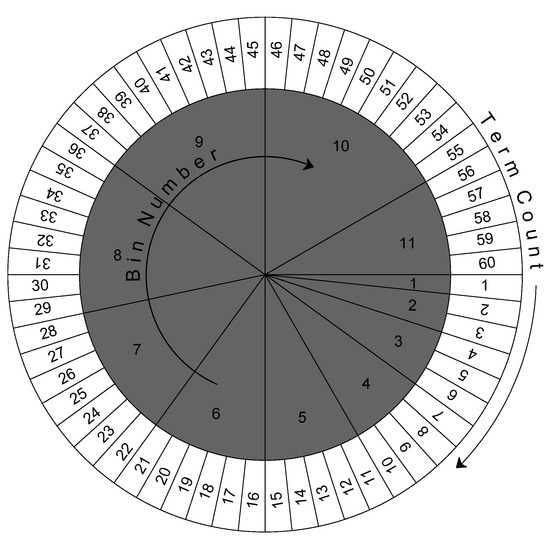
Figure 1. Mapping of term counts 1 to 60 to binned term counts.

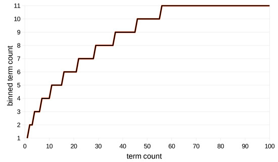
Figure 2. Mapping of term counts to binned term counts.

As BTC is a monotonically increasing function, it ensures that a term with lower term count in a document will not be mapped to a higher BTC value than its BTC value in another document having a higher term count. We hypothesize that reducing the document length in this way will reduce the anomaly discussed earlier in the previous subsection. Table 3 shows BTC mapping of term counts of the example given in Table 2. It can be seen that BTC maps higher term counts to higher or equal values than BTC values for lower term counts.

Table 3. BTC values of the terms given in Table 2.

Doc Id	Category	Label	Length	Term Count	TF (Equation (2))	BTC
2367	wheat	Multi	498	5	0.01	3
7154	grain	Single	167	2	0.01	2
(a) Frequencies of term ‘wheat’ in documents of wheat and grain categories
3981	grain	Multi	579	1	0.002	1
4679	cotton	Single	195	1	0.005	1
(b) Frequencies of term ‘grain’ in documents of grain and cotton categories

As discussed earlier in Table 2, in the scenario (a) term count of term ‘wheat’ in document 2367 of Reuters dataset is 5 and its term count in document 7154 is 2. Both term counts were mapped to TF = 0.01, although wheat’s term count is 2.5 times higher in one document than the other. BTC resolves this anomaly by mapping the term count 5 to BTC value 3 and term count 2 to BTC value 2. Hence, retaining the relative importance of the term ‘wheat’. BTC also resolved the anomaly discussed in scenario (b). Here, the term count of the term ‘grain’ is 1 in two different documents having document IDs 3981 and 4679 of Reuters dataset. TF frequency of grain in document of related class “grain” is lesser (0.002) than its term frequency in document of un-related class “cotton” (0.005). BTC maps both term counts to value 1, hence also resolving the second anomaly.

By mapping the elements that fall in a bin to one value, information is compressed, and the amount of compression increases with increase in bin size. Larger term counts are suppressed more than smaller term counts. We define the difference between a bin label and the average value of its elements as compression factor. Figure 3 shows the percentage compression for bin numbers.

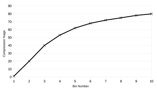
Figure 3. Percentage compression increases with increase in bin number. Higher term counts are being penalized more without affecting their importance.

3.3. Another Motivating Example

As reported in the literature, feature scaling is desirable for distance-based classification algorithms such as k-NN and SVM and clustering algorithms such as K-Means. Large values of features may result in large distances, making a classifier biased towards instances with large feature values. Although scaling is already being performed with document length normalized, the proposed BTC measure will further decrease unique values by mapping multiple values to a single bin. In this way, classifiers used to perform experiments should benefit from it.

Another example of the motivation of BTC is shown in Table 4, which contains a toy dataset with four terms and three documents. Document $d_1$ is a small document, $d_2$ is of medium length, while $d_3$ is a long document. The term counts and respective BTC values of the terms are tabulated. BTC imposes a maximum penalty on documents with large term counts ($d_3$), reducing document length from 76 to 24 (68% reduction). The small document ($d_1$) is least penalized (14%), while the medium length document ($d_2$) is imposed with 31% reduction. As BTC has reduced the length of large documents, it will reduce the anomalies introduced by document length normalization.

Table 4. Another motivating example.

Term Counts
Doc ID	$t_1$	$t_2$	$t_3$	$t_4$	Length
$d_1$	1	2	1	3	7
$d_2$	3	5	1	7	16
$d_3$	23	15	30	8	76
Binned Term Counts
$d_1$	1	2	1	2	6
$d_2$	3	3	1	4	11
$d_3$	7	5	8	4	24

Derivation of BTC Formula

In this section, we establish a mathematical relationship between term count and bin number. Bin numbers range from one to $\tau$ where $\tau$ is the threshold value. From Figure 1, we can see that a maximum term count $U_b$ in a bin b is sum of bin numbers $\left\{1,\dots ,b-2,b-1,b\right\}$. For example, the maximum term count in bin 4 is 10. Summing bin numbers 1, 2, 3, 4 gives 10. It is an arithmetic sequence with common difference $M=1$. We can represent $U_b$ as sum of arithmetic sequence as given by,

$$U_b=\frac{k(a_1+a_k)}{2}$$

(17)

where k is number of terms in the sequence, $a_1$ is the first term and $a_k$ is kth term. For the arithmetic sequence $\left\{1,\dots ,b-2,b-1,b\right\}$ with common difference $M=1$, $a_1=1$, $k=a_k=b$. Equation (17) becomes,

$$U_b=\frac{b(1+b)}{2}$$

(18)

Rearranging, we can obtain,

$$b^2+b-2U_b=0$$

(19)

This is a quadratic equation. Solving it for b and considering the positive part only, we obtain,

$$b=\frac{-1+\sqrt{1+8U_b}}{2}$$

(20)

Equation (20) is true if $U_b$ is the largest term count in the bin. Considering $U_b$ to be any arbitrary term count $tc$ in a bin, Equation (20) becomes an inequality.

$$b\ge \frac{-1+\sqrt{1+8tc}}{2}$$

(21)

As bin value b is an integer, rounding $R.H.S$ upwards to nearest integer will give us the actual value of b, which is given by,

$$b=\left[\frac{-1+\sqrt{1+8tc}}{2}\right]$$

(22)

Equation (22) defines the relationship between a term count $tc$ and bin b. Putting value of $tc$ in the above equation will give us the label of the bin where it should be mapped.

4. Empirical Evaluation

In this section, we explain the experimental setup used to compare the newly proposed BTC against the original TF and its more recently proposed alternative named modified term frequency (MTF) [55]. Each of these term frequency factors is used in conjunction with four well-known collection frequency factors namely IDF [56], RF [36], IGM [37], and MONO [39].

4.1. Description of the Datasets

We used three single labeled benchmark datasets for our experiments, namely R8 (a subset of Reuters-21578), WebKB and 20-Newsgroups. These datasets differ in size and class skew. Summary of the datasets is provided in Table 5. Reuters dataset is the most widely used dataset for text classification. We used the R8 version, which is already split into training and test sets using the modApté split. The other dataset is 20-Newsgroups that consists of newsgroup documents from 20 different categories. This dataset is known for its large size and balanced categories. This dataset has 18,821 documents in total. The last dataset is WebKB in which the documents correspond to web pages collected from different universities. This dataset is considered hard to classify due to its high sparsity. All three datasets were downloaded from Ana Cardoso Cachopo’s webpage [57] in raw text form.

Table 5. Summary of the datasets.

Dataset	Total Docs	Number of Terms	Number of Classes	Min Class Size	Max Class Size
Reuters (R8)	7674	7225	8	51	3923
Categories	acq, crude, earn, grain, interest, money-fx ship, trade
WebKB	4199	7105	4	504	1641
Categories	project, course, faculty, student
20 Newsgroups	18,821	29,739	20	628	999
Categories	talk.religion.misc,talk.politics.misc, alt.atheism,talk.politics.guns, talk.politics.mideast,comp.os.ms-windows.misc, comp.sys.mac.hardware, comp.graphics,misc.forsale, comp.sys.ibm.pc.hardware,sci.electronics, comp.windows.x,sci.space,rec.autos, sci.med,sci.crypt,rec.sport.baseball, rec.motorcycles, soc.religion.christian,rec.sport.hockey

4.2. Datasets Pre-Processing

We processed the datasets to generate term counts from raw text. We then applied stemming using Porter’s stemmer [58] and removed stop words using a stop words list. Pruning was applied afterwards to remove too rare and too frequent terms by applying lower and upper threshold values for document frequency. The values for upper and lower thresholds are the same as suggested by Forman in [59]. An absolute threshold value is used for lower threshold and words present in three or less documents are removed. For the upper threshold, we use a percentage of the total number of documents. The words present in 25% or more documents are removed. We used the training and test set splits as provided by the maintainers of the datasets.

4.3. Term Weighting Schemes

We compare the performance of two term frequency factors namely TF and MTF against our newly proposed BTC factor. Towards this end, we used 4 well-known collection frequency factors namely IDF [56], RF [36], IGM [37], and MONO [39]. In other words, we compare the performance of BTC-IDF, TF-IDF, and MTF-IDF on three datasets to find which factor (BTC, TF, or MTF) performs the best with the IDF factor. Similarly, we combine and compare BTC, TF and MTF with other factors. As recommended by [39], $\alpha$ in TF-MONO and $\gamma$ in TF-IGM should be set to 6 for the datasets of Reuters-21578 and WebKB while these coefficients should be set to 7 for 20 Newsgroups dataset. We used the same recommendations in our experiments. All these schemes were implemented in Python programming language.

4.4. Classification Algorithms

We used two classification algorithms, support vector machines (SVM) and K-nearest neighbors (KNN), to evaluate the text classification performance with the new BTC factor. SVM is a widely used classification algorithm in text classification [20]. We used the linear kernel of SVM from LibSVM package [60]. KNN is also well-known for its use in classifying text documents [61]. It is a simple learning algorithm and considers neighbor samples to classify documents. We tried different values of k for each dataset and found that 15, 11, and 20 produce better classification results for Reuters-21578, WebKB, and 20-Newsgroups datasets, respectively.

4.5. Evaluation Metrics

Macro-averaged $F_1$ is the most widely used measure to evaluate the classification performance of text classifiers [62]. The $F_1$-measure is a harmonic mean of precision and recall, where precision is ($p=\frac{tp}{tp+fp}$) and recall is ($r=\frac{tp}{tp+fn}$) [10]. Here, $tp$ denotes the true positives and $fp$ is the false positives while $fn$ denotes the false negatives. The macro $F_1$ can be calculated [63] as given by,

$$MacroAveraged{F}_1=\frac{{\displaystyle \sum _{j=1}^{\left|C\right|}}\frac{2\times p_j\times r_j}{p_j+r_j}}{\left|C\right|}$$

(23)

where $p_j$ is the precision and $r_j$ is the recall for jth class and $\left|C\right|$ is the number of classes in a dataset.

4.6. Evaluation Procedure

After a dataset is preprocessed, its terms are weighted by a term weighting scheme x.y, where x is one of the term frequency factors {TF, MTF, BTC} and y is one of the collection frequency factors {IDF, RF, IGM, MONO}. In our evaluation, we use CHI-square for selecting the most relevant terms as it is a well-known feature selection metric in text classification [37]. CHI-square is applied to the training set of a dataset to generate a list of terms or words in decreasing order of importance. Nested subsets are constructed by selecting the top 500, 1000, 2000, 4000, 6000, 8000, 10,000, 12,000, 14,000, and 16,000 ranked words for 20-Newsgroups and the top 100, 200, 500, 700, 1000, 2000, 3000, 4000, 5000, 6000, 7000 for R8 and WebKB datasets. Thus, we construct 10 nested subsets for 20-Newsgroups and 11 nested subsets for each of the R8 and WebKB datasets. The quality of each subset is investigated by training two classifiers (SVM and KNN) and measuring the macro $F_1$ values on the test set. These steps were repeated for the three datasets. Overall, there are 2 × (10 + 11 + 11) = 64 subsets for which BTC is compared against TF on three datasets with both the classifiers for a collection frequency factor. As we test four collection frequency factors, BTC and TF are compared in 4 × 64 = 256 nested subsets. The same holds for MTF too.

4.7. Statistical Analysis Procedure

To determine how significant is the performance of BTC, we repeat the above-mentioned evaluation procedure five times. For each of the five iterations, documents of a dataset are randomly split into training and test sets while maintaining the class skews. Given a classifier, for each nested subset,

• we obtain five different macro $F_1$ values for each term weighting scheme.
• we apply the paired two-sided t-test [64] on the macro $F_1$ values of BTC and those of its competing weighting scheme. The t-test is well-known for testing a null hypothesis of the means of two populations being equal (i.e., $H_0:{\mu }_1-{\mu }_2=0$ and $H_1:{\mu }_1-{\mu }_2\ne 0$) [65].
• we deduce the following information with the help of the 95% confidence interval (CI) values,

  (a)

  If CI values cross zero, the difference in the mean macro $F_1$ values is not significant. We consider this comparison to be a tie.

  (b)

  If CI does not cross zero, the difference between mean macro $F_1$ values is significant. We call this comparison a win for BTC if both lower and upper bounds of CI lie in the positive range, thus concluding that BTC’s performance is statistically better than that of its competitor. Otherwise, this comparison is a loss for BTC.

5. Results and Discussion

In this section, we present results with which we can compare performances of BTC, TF, and MTF on three datasets using SVM and KNN classifiers. There are four cases: TF-IGM vs BTC-IGM vs MTF-IGM, TF-IDF vs BTC-IDF vs MTF-IDF, TF-RF vs BTC-RF vs MTF-RF, TF-MONO vs BTC-MONO vs MTF-MONO. The tables presented contain the macro $F_1$. A win of BTC is depicted by a • symbol while a loss for BTC is indicated by a ∘. The absence of a symbol indicates a tie. For each dataset, the best classification performances with the smallest subset of top ranked terms are made bold and are also underlined. We use $\left|\mathbf{G}\right|$ to indicate cardinality of a subset that contains a certain number of top ranked terms.

5.1. BTC-IDF vs. TF-IDF vs. MTF-IDF

Table 6 shows the performance of BTC when used with IDF, which is the most widely used collection frequency factor for text classification. Either subsets of words are evaluated by SVM or KNN, we can find that BTC-IDF has achieved the highest macro $F_1$ values on all the three datasets. The analysis of t-test shows that BTC-IDF combination produces statistically better results than TF-IDF and MTF-IDF in most of the cases.

Table 6. Performance comparison of BTC-IDF vs TF-IDF vs MTF-IDF.

G	BTC-IDF	TF-IDF	MTF-IDF	BTC-IDF	TF-IDF	MTF-IDF
	SVM			KNN
	Reuters-21578 (R8)
100	86.1	86.9 ∘	84.3 •	84.9	83.5 •	83.7 •
200	89.4	88.9 •	86.5 •	87.4	86.2 •	86.4 •
500	90.3	89.3 •	89.7 •	88.1	86 •	86.8 •
700	90.5	89.7 •	89.5 •	$\underline{\mathbf{88}.\mathbf{6}}$	86.4 •	87.1 •
1000	90.7	89.9 •	89.9 •	87.8	85.8 •	85.9 •
2000	90.9	89.6 •	90 •	87.3	85.9 •	84.7 •
3000	90.9	89.7 •	90.2 •	87.6	86 •	84.7 •
4000	91.3	90 •	90.6 •	87	86 •	84.7 •
5000	91.3	90.2 •	90.7 •	86.9	85.6 •	84.8 •
6000	$\underline{\mathbf{91}.\mathbf{4}}$	89.9 •	90.6 •	87.2	85.3 •	84.7 •
7000	91.4	89.9 •	90.5 •	87.1	85.2 •	84.9 •
	WebKB
100	82.6	81.8 •	80 •	75.6	70.9 •	69.9 •
200	82.3	81.3 •	78.4 •	75.8	68.9 •	72.1 •
500	83	81 •	80.1 •	$\underline{\mathbf{76}.\mathbf{5}}$	70.9 •	74.5 •
700	83.3	81 •	80.1 •	75.4	70.4 •	74.5 •
1000	83.4	81.3 •	81 •	75.1	70.7 •	74.1 •
2000	84.4	81.5 •	80.8 •	74.3	70.6 •	72.8 •
3000	84.4	81.6 •	81.9 •	74.7	71.3 •	72.7 •
4000	84.9	81.8 •	81.9 •	74.8	71.5 •	73.2 •
5000	84.7	82.6 •	81.9 •	74.9	71 •	72.9 •
6000	84.9	83 •	82.4 •	74.9	71.5 •	73.3 •
7000	$\underline{\mathbf{85}.\mathbf{7}}$	83.4 •	83.6 •	74.9	70.9 •	72.3 •
	20-Newsgroups
500	70	68.9 •	68 •	69.9	66.2 •	67.2 •
1000	71.6	70.9 •	69.3 •	75	69.3 •	72 •
2000	73.8	72.8 •	71.8 •	78	72.6 •	74.9 •
4000	76.5	75.5 •	73.8 •	79.7	74.9 •	77.3 •
6000	78.8	77.7 •	75.7 •	80.7	75.8 •	78.1 •
8000	80	78.7 •	77.1 •	81.4	76.7 •	78.7 •
10,000	80.8	79.3 •	77.7 •	81.7	76.8 •	79.3 •
12,000	81.2	80 •	78.9 •	82	77.1 •	79.7 •
14,000	81.6	80.3 •	79.3 •	$\underline{\mathbf{82}.\mathbf{3}}$	77.3 •	79.8 •
16,000	$\underline{\mathbf{81}.\mathbf{9}}$	80.5 •	79.5 •	82.3	77.3 •	79.9 •

5.2. BTC-IGM vs. TF-IGM vs. MTF-IGM

The macro $F_1$ performance of BTC against that of TF and MTF is shown in Table 7 when IGM is used as the collection frequency factor. Application of t-test on the accuracies provide insight into the statistical significance of BTC. Results of BTC are better or comparable to those of TF and MTF. Moreover, BTC-IGM outperformed the other 2 term weighting schemes by exhibiting highest macro $F_1$ values on the three datasets.

Table 7. Performance comparison of BTC-IGM vs TF-IGM vs MTF-IGM.

G	BTC-IGM	TF-IGM	MTF-IGM	BTC-IGM	TF-IGM	MTF-IGM
	SVM			KNN
	Reuters-21578 (R8)
100	87.5	88.2 ∘	85.5 •	87.5	87.2 •	87.4 •
200	90	89.9 •	87.3 •	89.5	88.7 •	89.1 •
500	91.7	90.9 •	90 •	$\underline{\mathbf{91}.\mathbf{2}}$	89.7 •	90.7 •
700	91.6	90.9 •	90.7 •	91.2	89.4 •	90.8 •
1000	91.8	91.5 •	91.1 •	91.2	89.6 •	90.5 •
2000	92.3	92.1 •	91.7 •	90.6	88.9 •	90.4 •
3000	92.7	92.4 •	92 •	90.5	88.5 •	90.5
4000	93.1	92.6 •	92.5 •	90.7	88.6 •	90.5 •
5000	$\underline{\mathbf{93}.\mathbf{2}}$	92.6 •	92.6 •	90.8	88.6 •	90.7 •
6000	93.1	92.5 •	92.7 •	91	88.6 •	90.6 •
7000	93.2	92.3 •	92.7 •	90.8	88.5 •	90.7 •
	WebKB
100	82.7	81.7 •	80.7 •	77.6	73.6 •	72.8 •
200	82.8	81.9 •	80.4 •	80.1	75.7 •	77.5 •
500	84.3	82.7 •	82.5 •	81.2	76.8 •	80.9 •
700	85.2	83.7 •	82.8 •	80.9	76.5 •	80.5 •
1000	85.9	83.8 •	83.5 •	81.5	76.4 •	80.7 •
2000	86.2	84.4 •	83.2 •	81.2	76.3 •	80.2 •
3000	86.8	84.7 •	83.8 •	81.2	76.5 •	80.6 •
4000	86.9	84.8 •	83.9 •	81.7	76.5 •	80.8 •
5000	87.5	85.5 •	84 •	81.8	76.7 •	81 •
6000	87.9	85.6 •	84.7 •	$\underline{\mathbf{82}.\mathbf{2}}$	76.7 •	81.5 •
7000	$\underline{\mathbf{88}.\mathbf{8}}$	86.2 •	85.8 •	81.2	76.5 •	80.5 •
	20-Newsgroups
500	71.5	70.2 •	69.4 •	69.5	68.1 •	68.8 •
1000	74.2	73.2 •	71.7 •	74.6	72 •	73.9 •
2000	76.9	75.9 •	74.8 •	76.8	74.7 •	76.3 •
4000	79.3	78.4 •	77.7 •	79.3	77.3 •	77.8 •
6000	80.7	79.6 •	78.5 •	80.4	78.1 •	79.8 •
8000	81.5	80.5 •	79.4 •	80.9	78.7 •	79.7 •
10,000	82.1	81 •	79.8 •	81.2	78.9 •	80.4 •
12,000	82.5	81.2 •	80.5 •	81.6	79.1 •	80.7 •
14,000	82.6	81.3 •	80.8 •	81.7	79 •	80.9 •
16,000	$\underline{\mathbf{82}.\mathbf{8}}$	81.4 •	81 •	$\underline{\mathbf{82}}$	79.1 •	81 •

5.3. BTC-RF vs. TF-RF vs. MTF-RF

Results of evaluating the quality of subsets of BTC-RF, TF-RF and MTF-RF with SVM and KNN are shown in Table 8. The superior performance of BTC-RF weighting scheme is evident from the t-test analysis as compared to the other two schemes.

Table 8. Performance comparison of BTC-RF vs. TF-RF vs. MTF-RF.

G	BTC-RF	TF-RF	MTF-RF	BTC-RF	TF-RF	MTF-RF
	SVM			KNN
	Reuters-21578 (R8)
100	89	89	86.1 •	86.8	86.3 •	86 •
200	90.7	90.1 •	88 •	88.6	87.4 •	88.6
500	92	91.5 •	90.2 •	89.8	88.9 •	90.1 ∘
700	92.8	92 •	90.9 •	89.7	89 •	89.9 ∘
1000	92.9	91.9 •	91.2 •	89.9	89 •	90.3 ∘
2000	93	92.3 •	91.7 •	89.8	88.4 •	89.7 •
3000	92.8	92 •	91.8 •	$\underline{\mathbf{90}}$	88.4 •	89.9 •
4000	92.9	91.9 •	92.1 •	89.9	88.3 •	90.1 ∘
5000	93.1	92.1 •	92.2 •	89.9	88.6 •	90.2 ∘
6000	93.1	92.1 •	92.2 •	89.8	88.9 •	90.2 ∘
7000	$\underline{\mathbf{93}.\mathbf{2}}$	92.2 •	92.2 •	89.8	88.9 •	90.1 ∘
	WebKB
100	83.9	83 •	81.2 •	78.8	73.6 •	73.2 •
200	85.1	83.9 •	81.2 •	80	74.5 •	77.2 •
500	86.2	84.1 •	81.9 •	81.2	76.6 •	80 •
700	86.8	85.3 •	82.4 •	81.1	75.7 •	80.3 •
1000	86.8	85.4 •	82.9 •	81.3	75.8 •	80.4 •
2000	87.4	85.7 •	82.9 •	81.3	76.1 •	80.7 •
3000	87.6	86 •	83.5 •	81.5	76.4 •	80.6 •
4000	87.8	86.4 •	83.8 •	81.8	76.1 •	80.9 •
5000	88	86.4 •	84.5 •	$\underline{\mathbf{82}.\mathbf{1}}$	76.8 •	81 •
6000	88.3	86.4 •	85 •	82.1	76.2 •	81.2 •
7000	$\underline{\mathbf{88}.\mathbf{9}}$	86.9 •	86.2 •	81.7	75.6 •	80.5 •
	20-Newsgroups
500	73.1	71.8 •	71 •	70.7	68.2 •	68.7 •
1000	76.2	75.4 •	73.6 •	76.2	72.8 •	74.4 •
2000	78.3	77.5 •	76.1 •	77.9	75.2 •	76.4 •
4000	80.4	79.3 •	78.5 •	80.5	77.7 •	79 •
6000	81.5	80.5 •	79.5 •	82	78.2 •	80.5 •
8000	82.2	81.2 •	80.3 •	82.4	78.8 •	81 •
10,000	82.7	81.7 •	80.7 •	82.9	79 •	81.2 •
12,000	83	82 •	81.1 •	83.3	79.2 •	81.8 •
14,000	$\underline{\mathbf{83}.\mathbf{3}}$	82.3 •	81.5 •	$\underline{\mathbf{83}.\mathbf{6}}$	79.2 •	82 •
16,000	83.3	82.2 •	81.5 •	83.5	79.1 •	81.9 •

5.4. BTC-MONO vs. TF-MONO vs. MTF-MONO

Finally, we evaluate the capability of BTC, TF and MTF along with a more recently proposed collection frequency factor MONO. Table 9 shows the performance evaluations of the SVM and KNN classifiers. We can find that performance of BTC-MONO is better than that of the other two weighting schemes.

Table 9. Performance comparison of BTC-MONO vs. TF-MONO vs. MTF-MONO.

$\left|\mathbf{G}\right|$	BTC-MONO	TF-MONO	MTF-MONO	BTC-MONO	TF-MONO	MTF-MONO
	SVM			KNN
	Reuters-21578 (R8)
100	88	87.6 •	84.8 •	85.7	85.2 •	85.3 •
200	89.8	89.6 •	88.4 •	87.7	86.4 •	87.2 •
500	91.1	90.3 •	89.6 •	$\underline{\mathbf{88}.\mathbf{1}}$	87 •	87.8 •
700	91.5	90.5 •	90.3 •	88	86.7 •	87.8 •
1000	91.5	90.6 •	90.7 •	88	86.6 •	87.8 •
2000	91.6	91 •	90.9 •	88.1	86.6 •	87.8 •
3000	91.6	91.3 •	91.3 •	87.9	86.5 •	87.6 •
4000	91.8	91.3 •	91.4 •	87.9	86.4 •	87.6 •
5000	91.9	91.3 •	91.4 •	87.8	86.4 •	87.6 •
6000	91.9	91.2 •	91.3 •	87.8	86.4 •	87.5 •
7000	$\underline{\mathbf{92}}$	91.3 •	91.3 •	87.8	86.4 •	87.6 •
	WebKB
100	83	82.6 •	80.2 •	77.3	72.2 •	73.7 •
200	83.7	83.4 •	80 •	77.4	73.1 •	75.4 •
500	85	83 •	80.8 •	78.6	73.9 •	77.7 •
700	85.6	84.1 •	81.8 •	78.5	74.1 •	78.1 •
1000	85.6	84.1 •	82.5 •	78.7	73.9 •	78.4 •
2000	86.3	84.6 •	82.3 •	78.8	73.8 •	78.6 •
3000	86.5	85 •	82.7 •	78.5	74 •	78.6 ∘
4000	86.9	85.3 •	82.8 •	$\underline{\mathbf{78}.\mathbf{9}}$	73.9 •	79 ∘
5000	87.3	85.8 •	83.4 •	78.9	74 •	78.8 •
6000	87.2	85.9 •	84.2 •	78.9	74.2 •	79 ∘
7000	$\underline{\mathbf{87}.\mathbf{4}}$	86.3 •	84.7 •	78.7	73.8 •	78.6 •
	20-Newsgroups
500	70.8	70 •	68.9 •	61.6	59.7 •	60.7 •
1000	72.2	71.6 •	69.8 •	64.1	61.7 •	62.5 •
2000	73.6	72.4 •	70.9 •	65.3	62.1 •	63.7 •
4000	75	74.1 •	72.8 •	66.3	63.1 •	65.9 •
6000	76.2	75.4 •	74.5 •	67.1	63.1 •	66.7 •
8000	76.8	76.1 •	74.9 •	67.6	63.4 •	67.1 •
10,000	77.3	76.5 •	75.7 •	68	63.4 •	67.3 •
12,000	77.6	76.6 •	76.2 •	67.8	63.5 •	67.4 •
14,000	77.8	76.9 •	76.4 •	68	63.5 •	67.7 •
16,000	$\underline{\mathbf{78}.\mathbf{4}}$	77.1 •	76.7 •	$\underline{\mathbf{68}.\mathbf{3}}$	63.7 •	67.7 •

Our experimental results based on t-test lead us to a conclusion that both SVM and KNN classifiers achieve higher classification accuracies on the three standard datasets when BTC is used in combination with the collection frequency factors. Between the TF and MTF factors, BTC has won more trials against TF than MTF. The performance of BTC is better or comparable to TF and MTF while there is no loss for BTC.

5.5. Discussion of Results

Achieving high accuracy on unbalanced datasets is challenging for classification algorithms. In highly skewed datasets, more instances of smaller classes are misclassified than those of larger ones. A good classifier should be able to produce high macro $F_1$ values. This depends on the classification algorithm, a term weighting scheme, and a feature selection algorithm. Our focus in this paper is on the former. We investigated the working of our newly proposed BTC against TF and MTF while combining them with four collection frequency factors on three standard datasets with two classifiers. We used CHI-square to rank the terms and constructed 64 subsets for the three datasets. The results in Table 10 shows the count of subsets in which BTC has obtained performance statistically (over five splits of the datasets) better than TF and MTF on each dataset with each classifier. We can observe that performance of BTC is better than that of TF and MTF in 52% of the subsets. The remaining cases it is comparable to TF and MTF. There is no single subset for which the performance of BTC was poorer than that of TF and MTF.

Table 10. Summary: Percentage Wins of BTC against TF and MTF.

Data Set	IDF	RF	IGM	MONO	Row Total	Percentage	IDF	RF	IGM	MONO	Row Total	Percentage
	SVM						KNN
	TF
R8	8	6	1	1	16	36.4	5	2	9	10	26	59.1
WebKB	9	10	10	8	37	84.1	11	11	11	11	44	100
20NG	9	9	9	1	28	70	3	7	8	8	26	65
Col. Total	26	25	20	10	81	63.3	19	20	28	29	96	75
Percentage	81.3	78.1	62.5	31.3	63.3		59.4	62.5	87.5	90.6	75
	MTF
R8	2	5	3	0	10	22.7	11	1	0	0	12	27.3
WebKB	3	8	0	8	19	43.2	8	5	4	2	19	43.2
20NG	1	3	1	7	12	30	1	8	4	3	16	40
Col. Total	6	16	4	15	41	32	20	14	8	5	47	36.7
Percentage	18.8	50	12.5	46.9	32		62.5	43.8	25	15.6	36.7

Table 11 shows a summary of the highest macro $F_1$ values attained on each dataset. It can be seen that on the three datasets BTC-based term weighting schemes have been the top performer. BTC with IGM and RF have produced the highest macro $F_1$ values. On 20 newsgroup datasets, we found from the literature survey that one of the best macro $F_1$ results was reported in [63]. The SVM classifier obtained a macro $F_1$ value of 97.32. For the R8 dataset, [66] has reported one of the best macro $F_1$ results (i.e., 96.98) using SVM. Similarly, the macro $F_1$ value of 89.8 with Random forests classifier was found to be one of the best results on WebKB [67].

Table 11. Summary: Best Text Classification Results.

Data Set	Highest Value	Term Weighting Scheme	Highest Value	Term Weighting Scheme
	SVM		KNN
R8	93.2	BTC-IGM, BTC-RF	91.2	BTC-IGM
WebKB	88.9	BTC-RF	82.2	BTC-IGM
20NG	83.3	BTC-RF	83.6	BTC-RF

5.5.1. Strengths and Weaknesses of BTC

BTC, a non-linear weighting scheme, is designed to trim significant term counts more than small-term counts before normalization, thus helping to moderate the secondary effects produced on large documents. When all the documents in a dataset contain words with small term counts, researchers have suggested using binary values instead of term frequencies [10]. In such cases, BTC will only reduce term counts by a factor of 1 (assuming the maximum term count is 3). The resulting BTC values will be very close to the original term counts; hence, they will behave very similarly to TF. In case a corpus contains documents of almost equal length, documents cannot be distinguished as small and large documents. Therefore, the documents will be equally penalized by document length normalization. There is no need to alter term counts, instead, it may deteriorate the results. Moreover, if the threshold (the value after which all term counts will be mapped onto the max bin) needs to be set properly concerning term counts in a corpus, it will aggressively truncate term counts. In such cases, BTC may perform differently from expectations. BTC will perform well in situations other than those mentioned above. If the documents in a corpus vary mainly in size, BTC is a measure of choice in such cases. Also, as BTC scales the term counts, distance-based classifiers should benefit from it. Choosing a suitable threshold value is also crucial in determining overall performance.

5.5.2. Time Complexity of BTC

Regarding computational efficiency, the time complexity of Big-Oh of BTC, TF, and MTF is the same. If N is the number of terms, running time is $O\left(N\right)$. However, empirically, we found that, on average, TF, MTF, and BTC take 4 s, 755 s, and 3 s respectively. Therefore, BTC is computationally most efficient in finding the term weights of data. The system used in this experiment was HPZ420 with processor Intel Xeon 1660 (6 cores, 12 threads), 16 GB Ram, and 1TB solid state drive.

From the discussion above, we can conclude that BTC is better than TF and MTF in capturing a term’s importance at the document level. Therefore, when combined with a collection frequency factor, BTC performs better than TF and MTF.

6. Conclusions

In text classification, TF-IDF is the most commonly used term weighting scheme. TF being a measure of importance of term in a document employs normalization by the document length to make the larger terms counts in longer documents comparable to the term counts of shorter documents. However, this suppresses the term counts for longer documents more than term counts of shorter documents due to which a term’s true worth is not found. In this paper, we introduced a new term frequency factor named Binned Term Count (BTC), which eliminates the need of normalization by document length. BTC being an alternative to TF maps higher term counts to higher or equal values than mapped values of lower term counts. We evaluated performance of BTC on three benchmark datasets (namely Reuters-21578, 20 Newsgroups and WebKB) against TF and a more recently proposed alternative of TF using SVM and KNN classifiers. Based on two-sided paired t-test, our results showed that performance of BTC-based term weighting schemes is statistically significant than that of the TF- and MTF-based weighting schemes on all the three datasets. As a future work, BTC can be explored by introducing the variable length of the bins. These variable lengths may vary depending upon the average size of the documents in a corpus. In this way, length variation of the documents can be assigned in a controlled and effective manner.

References

- Sebastiani, F. Machine Learning in Automated Text Categorization. ACM Comput. Surv. 2002, 34, 1–47. [Google Scholar] [CrossRef]
- McManis, C.E.; Smith, D.A. Identifying Categories within Textual Data. U.S. Patent 10,157,178, 18 December 2018. [Google Scholar]
- HaCohen-Kerner, Y.; Rosenfeld, A.; Sabag, A.; Tzidkani, M. Topic-based classification through unigram unmasking. Procedia Comput. Sci. 2018, 126, 69–76. [Google Scholar] [CrossRef]
- Maruf, S.; Javed, K.; Babri, H.A. Improving text classification performance with random forests-based feature selection. Arab. J. Sci. Eng. 2016, 41, 951–964. [Google Scholar] [CrossRef]
- Li, L.; Xiao, L.; Jin, W.; Zhu, H.; Yang, G. Text Classification Based on Word2vec and Convolutional Neural Network. In Proceedings of the International Conference on Neural Information Processing, Siem Reap, Cambodia, 13–16 December 2018; Springer: Berlin/Heidelberg, Germany, 2018; pp. 450–460. [Google Scholar]
- Sidorov, G. Generalized n-grams. In Syntactic n-Grams in Computational Linguistics; Springer: Berlin/Heidelberg, Germany, 2019; pp. 85–86. [Google Scholar]
- Li, Y.J.; Chung, S.M.; Holt, J.D. Text document clustering based on frequent word meaning sequences. Data Knowl. Eng. 2008, 64, 381–404. [Google Scholar] [CrossRef]
- Yao, L.; Mao, C.; Luo, Y. Graph convolutional networks for text classification. In Proceedings of the AAAI Conference on Artificial Intelligence, Honolulu, HI, USA, 27 January–1 February 2019; Volume 33, pp. 7370–7377. [Google Scholar]
- Wang, R.; Chen, G.; Sui, X. Multi label text classification method based on co-occurrence latent semantic vector space. Procedia Comput. Sci. 2018, 131, 756–764. [Google Scholar] [CrossRef]
- Forman, G. An extensive empirical study of feature selection metrics for text classification. J. Mach. Learn. Res. 2003, 3, 1289–1305. [Google Scholar]
- Lan, M.; Sung, S.Y.; Low, H.B.; Tan, C.L. A comparative study on term weighting schemes for text categorization. In Proceedings of the IEEE International Joint Conference on Neural Networks, Montreal, QC, Canada, 31 July–4 August 2005; pp. 546–551. [Google Scholar]
- Sinoara, R.A.; Camacho-Collados, J.; Rossi, R.G.; Navigli, R.; Rezende, S.O. Knowledge-enhanced document embeddings for text classification. Knowl. -Based Syst. 2019, 163, 955–971. [Google Scholar] [CrossRef]
- Salton, G.; Buckley, C. Term-weighting Approaches in Automatic Text Retrieval. Inf. Process. Manag. 1988, 24, 513–523. [Google Scholar] [CrossRef]
- Leopold, E.; Kindermann, J. Text Categorization with Support Vector Machines. How to Represent Texts in Input Space? Mach. Learn. 2002, 46, 423–444. [Google Scholar] [CrossRef]
- Haddoud, M.; Mokhtari, A.; Lecroq, T.; Abdeddaïm, S. Combining supervised term-weighting metrics for SVM text classification with extended term representation. Knowl. Inf. Syst. 2016, 49, 909–931. [Google Scholar] [CrossRef]
- Liu, Y.; Loh, H.T.; Toumi, K.Y.; Tor, S.B. Handling of Imbalanced Data in Text Classification: Category-Based Term Weights. In Natural Language Processing and Text Mining; Springer: London, UK, 2007; pp. 172–192. [Google Scholar]
- Zhang, T.; Ge, S.S. An Improved TF-IDF Algorithm Based on Class Discriminative Strength for Text Categorization on Desensitized Data. In Proceedings of the 2019 3rd International Conference on Innovation in Artificial Intelligence, ACM, New York, NY, USA, 15–18 March 2019; pp. 39–44. [Google Scholar]
- Dogan, T.; Uysal, A.K. On Term Frequency Factor in Supervised Term Weighting Schemes for Text Classification. Arab. J. Sci. Eng. 2019, 44, 9545–9560. [Google Scholar] [CrossRef]
- Chen, L.; Jiang, L.; Li, C. Using modified term frequency to improve term weighting for text classification. Eng. Appl. Artif. Intell. 2021, 101, 104215. [Google Scholar] [CrossRef]
- Sabbah, T.; Selamat, A.; Selamat, M.H.; Al-Anzi, F.S.; Viedma, E.H.; Krejcar, O.; Fujita, H. Modified frequency-based term weighting schemes for text classification. Appl. Soft Comput. 2017, 58, 193–206. [Google Scholar] [CrossRef]
- Singhal, A.; Salton, G.; Buckley, C. Length Normalization in Degraded Text Collections. In Proceedings of the Fifth Annual Symposium on Document Analysis and Information Retrieval, Las Vegas, NV, USA, 15–17 April 1995; pp. 15–17. [Google Scholar]
- Singhal, A.; Buckley, C.; Mitra, M. Pivoted document length normalization. In Proceedings of the ACM SIGIR Forum, Tokyo, Japan, 7–11 August 2017; Volume 51, pp. 176–184. [Google Scholar]
- Nigam, K.; Mccallum, A.K.; Thrun, S.; Mitchell, T. Text Classification from Labeled and Unlabeled Documents using EM. Mach. Learn. 2000, 39, 103–134. [Google Scholar] [CrossRef]
- Ponte, J.M.; Croft, W.B. A Language Modeling Approach to Information Retrieval. In Proceedings of the 21st Annual International ACM SIGIR Conference on Research and Development in Information Retrieval, Melbourne, Australia, 24–28 August 1998; pp. 275–281. [Google Scholar]
- Xue, X.B.; Zhou, Z.H. Distributional Features for Text Categorization. IEEE Trans. Knowl. Data Eng. 2009, 21, 428–442. [Google Scholar]
- Sabbah, T.; Selamat, A. Modified frequency-based term weighting scheme for accurate dark web content classification. In Proceedings of the Asia Information Retrieval Symposium; Springer: Berlin/Heidelberg, Germany, 2014; pp. 184–196. [Google Scholar]
- Arunachalam, A.; Aruldevi, M.; Perumal, S. An Efficient Document Search in Web Learning using Term Frequency and Inverse Document Frequency. Int. J. Pure Appl. Math. 2018, 119, 3739–3747. [Google Scholar]
- Joho, H.; Sanderson, M. Document frequency and term specificity. In Proceedings of the RIAO ’07 Large Scale Semantic Access to Content (Text, Image, Video, and Sound), Pittsburgh, PA, USA, 30 May–1 June 2007; pp. 350–359. [Google Scholar]
- Anandarajan, M.; Hill, C.; Nolan, T. Term-Document Representation. In Practical Text Analytics; Springer: Berlin/Heidelberg, Germany, 2019; pp. 61–73. [Google Scholar]
- Bafna, P.; Pramod, D.; Vaidya, A. Document clustering: TF-IDF approach. In Proceedings of the 2016 International Conference on Electrical, Electronics, and Optimization Techniques (ICEEOT), Chennai, India, 3–5 March 2016; pp. 61–66. [Google Scholar]
- Debole, F.; Sebastiani, F. Supervised term weighting for automated text categorization. In Text Mining and Its Applications; Springer: Berlin/Heidelberg, Germany, 2004; pp. 81–97. [Google Scholar]
- Lertnattee, V.; Theeramunkong, T. Analysis of inverse class frequency in centroid-based text classification. In Proceedings of the IEEE International Symposium on Communications and Information Technology—ISCIT 2004, Sapporo, Japan, 26–29 October 2004; Volume 2, pp. 1171–1176. [Google Scholar]
- Wang, D.; Zhang, H. Inverse-category-frequency based supervised term weighting scheme for text categorization. J. Inf. Sci. Eng. 2013, 29, 209–225. [Google Scholar]
- Quan, X.; Wenyin, L.; Qiu, B. Term weighting schemes for question categorization. IEEE Trans. Pattern Anal. Mach. Intell. 2010, 33, 1009–1021. [Google Scholar] [CrossRef]
- Ren, F.; Sohrab, M.G. Class-indexing-based term weighting for automatic text classification. Inf. Sci. 2013, 236, 109–125. [Google Scholar] [CrossRef]
- Lan, M.; Tan, C.L.; Su, J.; Lu, Y. Supervised and traditional term weighting methods for automatic text categorization. IEEE Trans. Pattern Anal. Mach. Intell. 2009, 31, 721–735. [Google Scholar] [CrossRef]
- Chen, K.; Zhang, Z.; Long, J.; Zhang, H. Turning from TF-IDF to TF-IGM for term weighting in text classification. Expert Syst. Appl. 2016, 66, 245–260. [Google Scholar] [CrossRef]
- Dogan, T.; Uysal, A.K. Improved inverse gravity moment term weighting for text classification. Expert Syst. Appl. 2019, 130, 45–59. [Google Scholar] [CrossRef]
- Dogan, T.; Uysal, A.K. A novel term weighting scheme for text classification: TF-MONO. J. Inf. 2020, 14, 101076. [Google Scholar] [CrossRef]
- Mikolov, T.; Sutskever, I.; Chen, K.; Corrado, G.S.; Dean, J. Distributed Representations of Words and Phrases and their Compositionality. In Proceedings of the Advances in Neural Information Processing Systems, Lake Tahoe, NV, USA, 5–8 December 2013; Volume 26. [Google Scholar]
- Devlin, J.; Chang, M.; Lee, K.; Toutanova, K. BERT: Pre-training of Deep Bidirectional Transformers for Language Understanding. In Proceedings of the 2019 Conference of the North American Chapter of the Association for Computational Linguistics: Human Language Technologies, NAACL-HLT 2019, Minneapolis, MN, USA, 2–7 June 2019; Volume 1, pp. 4171–4186. [Google Scholar]
- Ge, L.; Moh, T.S. Improving text classification with word embedding. In Proceedings of the 2017 IEEE International Conference on Big Data (Big Data), Boston, MA, USA, 11–14 November 2017; pp. 1796–1805. [Google Scholar]
- Di Gennaro, G.; Buonanno, A.; Palmieri, F. Considerations about learning Word2Vec. J. Supercomput. 2021, 77, 12320–12335. [Google Scholar] [CrossRef]
- Jatnika, D.; Bijaksana, M.A.; Suryani, A.A. Word2vec model analysis for semantic similarities in English words. Procedia Comput. Sci. 2019, 157, 160–167. [Google Scholar] [CrossRef]
- Ordentlich, E.; Yang, L.; Feng, A.; Cnudde, P.; Grbovic, M.; Djuric, N.; Radosavljevic, V.; Owens, G. Network-efficient distributed word2vec training system for large vocabularies. In Proceedings of the 25th Acm International on Conference on Information and Knowledge Management, Indianapolis, IN, USA, 24–28 October 2016; pp. 1139–1148. [Google Scholar]
- Pennington, J.; Socher, R.; Manning, C.D. GloVe: Global Vectors for Word Representation. In Proceedings of the EMNLP, Doha, Qatar, 25–29 October 2014; Volume 14, pp. 1532–1543. [Google Scholar]
- Joulin, A.; Grave, E.; Bojanowski, P.; Mikolov, T. Bag of Tricks for Efficient Text Classification. arXiv 2016, arXiv:1607.01759. [Google Scholar]
- Koroteev, M.V. BERT: A Review of Applications in Natural Language Processing and Understanding. arXiv 2021, arXiv:2103.11943. [Google Scholar]
- Li, Q.; Zhang, Y.; Wang, H. Knowledge Base Question Answering for Intelligent Maintenance of Power Plants. In Proceedings of the 2021 IEEE 24th International Conference on Computer Supported Cooperative Work in Design (CSCWD), Dalian, China, 5–7 May 2021; pp. 626–631. [Google Scholar]
- Yu, S.; Su, J.; Luo, D. Improving BERT-Based Text Classification With Auxiliary Sentence and Domain Knowledge. IEEE Access 2019, 7, 176600–176612. [Google Scholar] [CrossRef]
- Smith, N.A. Contextual word representations: Putting words into computers. Commun. ACM 2020, 63, 66–74. [Google Scholar] [CrossRef]
- Qiu, Y.; Yang, B. Research on Micro-blog Text Presentation Model Based on Word2vec and TF-IDF. In Proceedings of the 2021 IEEE Asia-Pacific Conference on Image Processing, Electronics and Computers (IPEC), Dalian, China, 14–16 April 2021; pp. 47–51. [Google Scholar]
- Zhu, D.; Wong, K.W. An evaluation study on text categorization using automatically generated labeled dataset. Neurocomputing 2017, 249, 321–336. [Google Scholar] [CrossRef]
- Flach, P. Machine Learning: The Art and Science of Algorithms That Make Sense of Data; Cambridge University Press: New York, NY, USA, 2012. [Google Scholar]
- Chen, L.; Jiang, L.; Li, C. Modified DFS-based term weighting scheme for text classification. Expert Syst. Appl. 2021, 168, 114438. [Google Scholar] [CrossRef]
- Jones, K.S. A statistical interpretation of term specificity and its application in retrieval. J. Doc. 2004, 40, 493–502. [Google Scholar] [CrossRef]
- Cachopo, A.M.J.C. Improving Methods for Single-Label Text Categorization. Ph.D. Thesis, Instituto Superior Tecnico, Universidade Tecnica de Lisboa, Lisboa, Portugal, 2007. [Google Scholar]
- Willett, P. The Porter stemming algorithm: Then and now. Program: Electron. Libr. Inf. Syst. 2006, 40, 219–223. [Google Scholar] [CrossRef]
- Forman, G. A pitfall and solution in multi-class feature selection for text classification. In Proceedings of the Twenty-First International Conference on Machine Learning, Banff, AB, Canada, 4–8 July 2004; p. 38. [Google Scholar]
- Chang, C.C.; Lin, C.J. LIBSVM: A library for support vector machines. ACM Trans. Intell. Syst. Technol. (TIST) 2011, 2, 1–27. [Google Scholar] [CrossRef]
- Sabbah, T.; Selamat, A.; Selamat, M.H.; Ibrahim, R.; Fujita, H. Hybridized term-weighting method for dark web classification. Neurocomputing 2016, 173, 1908–1926. [Google Scholar] [CrossRef]
- Asim, M.; Javed, K.; Rehman, A.; Babri, H. A new feature selection metric for text classification: Eliminating the need for a separate pruning stage. Int. J. Mach. Learn. Cybern. 2021, 12, 2461–2478. [Google Scholar] [CrossRef]
- Uysal, A.K.; Gunal, S. A novel probabilistic feature selection method for text classification. Knowl. -Based Syst. 2012, 36, 226–235. [Google Scholar] [CrossRef]
- Navidi, W. Statistics for Engineers and Scientists, 4th ed.; McGraw-Hill Education: New York, NY, USA, 2015. [Google Scholar]
- Witte, R.S.; Witte, J.S. Statistics, 9th ed.; John Wiley & Sons: Hoboken, NJ, USA, 2010. [Google Scholar]
- Goudjil, M.; Koudil, M.; Bedda, M.; Ghoggali, N. A Novel Active Learning Method Using SVM for Text Classification. Int. J. Autom. Comput. 2018, 15, 290–298. [Google Scholar] [CrossRef]
- Ali, M.S.; Javed, K. A Novel Inherent Distinguishing Feature Selector for Highly Skewed Text Document Classification. Arab. J. Sci. Eng. 2020, 45, 10471–10491. [Google Scholar] [CrossRef]
Publisher’s Note: MDPI stays neutral with regard to jurisdictional claims in published maps and institutional affiliations. |
© 2022 by the authors. Licensee MDPI, Basel, Switzerland. This article is an open access article distributed under the terms and conditions of the Creative Commons Attribution (CC BY) license (https://creativecommons.org/licenses/by/4.0/).