Boundary Feedback Stabilization of Two-Dimensional Shallow Water Equations with Viscosity Term

Abstract

This paper treats a water flow regularization problem by means of local boundary conditions for the two-dimensional viscous shallow water equations. Using an a-priori energy estimate of the perturbation state and the Faedo–Galerkin method, we build a stabilizing boundary feedback control law for the volumetric flow in a finite time that is prescribed by the solvability of the associated Cauchy problem. We iterate the same approach to build by cascade a stabilizing feedback control law for infinite time. Thanks to a positive arbitrary time-dependent stabilization function, the control law provides an exponential decay of the energy.

1. Introduction

Regularization of free-surface fluid flows is a problem of practical interest for environmental and budgetary purposes in the current situation of climate change that rarefies fresh water sources worldwide. Depending on the specific application, the regularization of fluid flows is performed through control methodologies of the Navier–Stokes equations or a system of partial differential equations derived from them, which describe a particular setting and/or physical properties. Several mechanisms of controlling fluid flows have been designed in the recent past, see [1,2,3,4,5].

Control and stabilization of fluid flows governed by the Navier–Stokes equations have been extensively studied in the literature using various approaches. In the three-dimensional setting, a local stabilization around an unstable stationary state is performed in [6] by means of a feedback control law. In [7], the existence of time-points values of boundary feedback laws is achieved by an optimal control problem to alleviate the high regularity required for the velocity components. One of the widely adopted approaches formulates the associate optimal control problem in infinite dimensional spaces, which gives rise to a Riccati equation [8]. Stabilization of the Navier-Stokes equations from the boundary or from a portion of the boundary is mainly investigated by means of feedback control laws. In addition to the series of papers [9,10,11,12,13], the inclusive examination in [14] lists a number of approaches for control by means of feedback laws. It also discusses the associated challenges, such as start-control, impulse-control and distributed-control laws, which have been studied for the Oseen and Navier-Stokes equations. Recently, global solution as well as an optimality system and a second-order sufficient optimality condition were obtained for the stationary two-dimensional Stokes equations [15,16], while an optimal controllability of a stationary two-dimensional non-Newtonian fluid in a pipeline network is studied in [17].

When the horizontal length scale of the physical domain is much greater than the vertical one, the flow movement can be captured by the water height and the horizontal velocity field. In that particular setting of shallow water flows, great advances have been made in the mechanism of controlling free-surface flow parameters by local boundary conditions, despite the challenges associated with the nonlinearity of the governing equations, see [18,19] for detailed and comprehensive reviews. Global stability of the two-dimensional water flow has been achieved in $L^2$-norm [20] using the symmetrization of the flux matrices, in $H^2$-norm [21], by acting on the tangential velocity. The approach of tracking the flow energy through the Riemann invariant variables is adopted in [22,23] in the one-dimensional setting and is explored in [24] for the two-dimensional channel flow. Besides the provided flexibility in practical experiments, the adding of the viscosity influence provides regularizing effects in estimating the flow energy, see [25].

In this paper, we address the stabilization of two-dimensional viscous shallow water around a steady-state, that is, the problem of driving the flow-state variables of viscous incompressible fluid inside a bounded container to a desired steady state. The control law acts on the volumetric flow vector along a portion of the boundary. Due to the challenges inherent in dealing with the nonlinear advection, we alleviate the nonlinearity issues by processing to the linearization around the steady state for small perturbations of the flow state. The resulting system of linear partial differential equations is referred to as the linearized shallow-water model, for which the existence and the uniqueness of solution is addressed by combining some notions of compactness and an a-priori energy estimate using the Faedo-Galerkin method. Subsequently, the stabilization of the nonlinear model around the steady state is rearranged as the stabilization of the linearized model around zero. In a short time, prescribed by the existence of a solution to the Cauchy problem associated with the weak formulation in an Hilbertian basis, the control building process explores only the estimation of the non-viscous energy of the linearized model and relies on a continuous time-dependent stabilization rate. The global-time stabilization result is established by cascading over a sequence of intervals.

The content of this paper is organized as follows: Section 2 introduces the equations governing the flow of a viscous shallow water in a three-dimensional domain with a given bathymetry. In Section 3, we detail the problem setting: we present the steady-state model, discuss the linearization, set the notations and the assumptions of the function spaces, and state the stabilization problem. Section 4 is devoted to the design of the small-time feedback control law. The main result of the stabilization of the linearized shallow-water model through the exponential decay of the energy is presented in Section 5. We conclude by giving some perspective directions of improvement of the presented method in Section 6.

2. 2-D Viscous Shallow-Water Equations

Consider a three-dimensional domain with a non-flat bottom in which a viscous water flows with a free-surface denoted by $\Omega$, a bounded subset of ${\mathbb{R}}^2$, with boundary $\partial \Omega ={\Gamma }_1\cup {\Gamma }_2$. The SWE (shallow-water equations) are a set of partial differential equations derived by depth integrating the Navier–Stokes equations, see [26,27,28,29], with the assumption that the horizontal length scale of the domain is much greater than the vertical one. In the absence of Coriolis, frictional, and wind effects, the 2D viscous SWE with a viscosity coefficient $\mu$ in $[m^2·s^{-1}]$ are given by

$$\begin{array}{c}\hfill \left\{\begin{array}{cc}{\displaystyle {\partial }_{t}H+{\partial }_x\left(H{V}_{{}_1}\right)+{\partial }_y\left(H{V}_{{}_2}\right)=0}\hfill & {\displaystyle \mathrm{in}\mathcal{Q},}\hfill \\ {\displaystyle {\partial }_t\left(H{V}_{{}_1}\right)+{\partial }_x\left(H{V}_{{}_1}^2\right)+gH{\partial }_x\left(H+\eta \right)+{\partial }_y\left(H{V}_{{}_1}{V}_{{}_2}\right)=\mu \Delta \left(H{V}_{{}_1}\right)}\hfill & {\displaystyle \mathrm{in}\mathcal{Q},}\hfill \\ {\displaystyle {\partial }_t\left(H{V}_{{}_2}\right)+{\partial }_x\left(H{V}_{{}_1}{V}_{{}_2}\right)+{\partial }_y\left(H{V}_{{}_2}^2\right)+gH{\partial }_y\left(H+\eta \right)=\mu \Delta \left(H{V}_{{}_2}\right)}\hfill & {\displaystyle \mathrm{in}\mathcal{Q},}\hfill \\ {\displaystyle \left(H,V_{{}_1},V_{{}_2}\right)(0,·,·)=\left(H^0,V_{{}_1}^0,V_{{}_2}^0\right)(·,·)}\hfill & {\displaystyle \mathrm{in}\Omega ,}\hfill \\ \mathrm{boundary}\mathrm{conditions}\mathrm{to}\mathrm{be}\mathrm{specified},\hfill \end{array}\right.\end{array}$$

(1)

where $\mathcal{Q}=(0,T)\times \Omega$, $T>0$ denotes the duration of the study, H the height of the water column, $\left(V_{{}_1},V_{{}_2}\right)$ the velocity vector with reference to $(Ox,Oy)$, $\eta$ the bathymetry describing the bottom elevation, and g is the constant of the acceleration due to the gravity force. The symbol ${\partial }_t$ designates the time derivative while ${\partial }_x$ and ${\partial }_y$ are the space derivatives in the x-direction and y-direction, respectively. The differential operator $\Delta$ represents the diffusion field $\Delta ={\partial }_{xx}+{\partial }_{yy}$. The triplet $\left(H,V_{{}_1},V_{{}_2}\right)$ varies with $(t,x,y)$ and forms the solution of (1) while the bathymetry $\eta (x,y)$ is independent of the time variable because there is no sediment transport. For the unidirectional propagation, an alternative approach to describing the waves at the free surface of shallow water under the influence of gravity is to consider the Korteweg–de Vries equation, see [30], where notions in differential geometry help to establish the existence of global solutions, see [31].

The diffusion effects have been modeled in several ways in the literature. It is shown in [32] that the formulation $\mu H\Delta V_{{}_i}$ on the right hand side of (1) is not consistent with the primitive form of the equations for the energy norm and an energetically consistent formulation is given therein. This is deeply analyzed through the existence of weak solutions to the SWE in [33], where, by looking for $(V_{{}_1},V_{{}_2})$ bounded in $L^2(0,T,H^1(\Omega ))$, $H\in L^{\infty }(0,T,L^1(\Omega ))$ and $HlogH\in L^{\infty }(0,T,L^1(\Omega ))$ to induce the dissipation, the term $H{V}_{{}_i}$ stands as an obstacle for the existence of solutions. That is why there is a constraint of small data to guarantee the existence of time-local weak solutions.

For the diffusion formulation $\mu \Delta \left(H{V}_{{}_i}\right)$, as used here on the right hand side of (1), the existence of weak solutions and its stability are described in [26]. In that case, the diffusion provides regularizing effects due to an entropic inequality on the height variable H. It is important to notice that the stability result is restricted to the models where capillarity and friction are taken into account. For the 1-D model, a clearer result for the existence of weak global solutions can be elaborated with much less restrictive data [33].

Using the volumetric flow variable vector $\mathbf{Q}=(Q_{{}_1},Q_{{}_2})=(H{V}_{{}_1},H{V}_{{}_2})$, the system (1) is rewritten for further analysis in the following conservative form:

$$\begin{array}{c}\hfill \begin{array}{ccc}& {\partial }_{t}H+\mathrm{div}\mathbf{Q}=0,\hfill & {\displaystyle \mathrm{in}\mathcal{Q},}\hfill \\ & {\partial }_t\mathbf{Q}+\mathrm{div}\mathcal{F}(H,\mathbf{Q})+gH\nabla (H+\eta )-\mu \Delta \mathbf{Q}=0,\hfill & {\displaystyle \mathrm{in}\mathcal{Q},}\hfill \end{array}\end{array}$$

(2)

where $\mathbf{Q}={\left(Q_{{}_1},Q_{{}_2}\right)}^{\top }$ (the superscript ⊤ is the transpose operator), the matrix $\mathcal{F}(H,\mathbf{Q})=\mathbf{Q}·{\mathbf{Q}}^{\top }/H$, the differential operator ∇ is the gradient field, and div(·) stands for the divergence operator, div($\mathit{f}$) = $\nabla ·\mathit{f}$ for a sufficiently regular vector function. Although the non-conservative formulation, see [20], is known to provide a better mass conservation of the volumetric quantity of water, it does not hold across a shock or a hydraulic jump since velocities do not generate fundamental conservation equations. On the other hand, the conservative formulation (2) supports front discontinuities such as shock waves at a fluid’s interface and irregular source terms, and appeals to Riemann solver for numerical resolution, see [22,23,34,35]. Therefore, the conservative form (2) is well-suited for our stabilization problem, which we state in the next section.

3. Statement of the Problem

In this section, we lay out the stabilization problem from the linearization around the steady state to the setting of finding the boundary feedback control law.

3.1. Steady-State, Linearization

The objective of the stabilization is to bring the variables of the flow to a given steady state that is the reference state. In practice, this consists of finding a controller (inflows, outflows) allowing to adjust the flow parameters to keep the flow state variables near this reference state. We denote the steady state by $\overline{\mathit{U}}={(\overline{h},{\overline{q}}_{{}_1},{\overline{q}}_{{}_2})}^{\top }$ and it is stationary and given by:

$$\begin{array}{c}\hfill \begin{array}{ccc}& \mathrm{div}\overline{\mathit{q}}=0,\hfill & {\displaystyle \mathrm{in}\Omega ,}\hfill \\ & g\overline{h}\nabla \left(\overline{h}+\eta \right)-\frac{1}{\overline{h}}\mathcal{F}(\overline{h},\overline{\mathit{q}})·\nabla \overline{h}+\frac{1}{\overline{h}}(\nabla \overline{\mathit{q}})·\overline{\mathit{q}}-\mu \Delta \overline{\mathit{q}}=0\hfill & {\displaystyle \mathrm{in}\Omega .}\hfill \end{array}\end{array}$$

(3)

The hydrodynamical variable vector $(H,Q_{{}_1},Q_{{}_2})$ is formed by the equilibrium state $(\overline{h},{\overline{q}}_{{}_1},{\overline{q}}_{{}_2})$ and a perturbation state denoted by $(h,q_{{}_1},q_{{}_2})$. Hence, the linearization consists of using

$$\begin{array}{c}\hfill \begin{array}{c}H(t,x,y)=\overline{h}(x,y)+h(t,x,y),\\ Q_{{}_1}(t,x,y)={\overline{q}}_{{}_1}(x,y)+q_{{}_1}(t,x,y),\\ Q_{{}_2}(t,x,y)={\overline{q}}_{{}_2}(x,y)+q_{{}_2}(t,x,y).\end{array}\end{array}$$

(4)

We proceed to the linearization of the system (2) by replacing the state variables H, $Q_{{}_1}$ and $Q_{{}_2}$ by their above expressions. In addition, we consider the following assumption $\left|h\right|\ll \overline{h}$, $\left|q_{{}_1}\right|\ll \left|{\overline{q}}_{{}_1}\right|$ and $\left|q_{{}_2}\right|\ll \left|{\overline{q}}_{{}_2}\right|$ to justify keeping only the first-order terms in the perturbation state because we neglect higher order terms. We denote by

$$\begin{array}{c}\hfill \overline{\mathit{v}}=\left(\begin{array}{c}{\displaystyle {\overline{v}}_{{}_1}}\\ \\ {\displaystyle {\overline{v}}_{{}_2}}\end{array}\right),{\mathbf{\alpha }}_{{}_0}=\left(\begin{array}{c}{\displaystyle {\alpha }_{{}_0}^1}\\ \\ {\displaystyle {\alpha }_{{}_0}^2}\end{array}\right),\mathit{A}=\left(\begin{array}{cc}{\displaystyle {\beta }_{{}_0}^1}& {\displaystyle {\gamma }_{{}_0}^1}\\ \\ {\displaystyle {\beta }_{{}_0}^2}& {\displaystyle {\gamma }_{{}_0}^2}\end{array}\right),\mathrm{and}\mathit{B}=\left(\begin{array}{cc}{\displaystyle {\alpha }_{{}_1}^1}& {\displaystyle {\alpha }_{{}_2}^1}\\ \\ {\displaystyle {\alpha }_{{}_1}^2}& {\displaystyle {\alpha }_{{}_2}^2}\end{array}\right),\end{array}$$

where the coefficients are given by:

$$\begin{array}{ccccc}\hfill {\alpha }_{{}_0}^1& =g{\partial }_x\overline{h}+g{\partial }_x\eta ,\hfill & \hfill {\alpha }_{{}_0}^2& =g{\partial }_y\overline{h}+g{\partial }_y\eta ,\hfill & \\ \hfill {\beta }_{{}_0}^1& =\frac{1}{\overline{h}}\left(2{\partial }_x{\overline{q}}_{{}_1}-2{\overline{v}}_{{}_1}{\partial }_x\overline{h}+{\partial }_y{\overline{q}}_{{}_2}-{\overline{v}}_{{}_2}{\partial }_y\overline{h}\right),\hfill & \hfill {\beta }_{{}_0}^2& =\frac{1}{\overline{h}}\left({\partial }_x{\overline{q}}_{{}_2}-{\overline{v}}_{{}_2}{\partial }_x\overline{h}\right),\hfill & \\ \hfill {\gamma }_{{}_0}^1& =\frac{1}{\overline{h}}\left({\partial }_y{\overline{q}}_{{}_1}-{\overline{v}}_{{}_1}{\partial }_y\overline{h}\right),\hfill & \hfill {\gamma }_{{}_0}^2& =\frac{1}{\overline{h}}\left(2{\partial }_y{\overline{q}}_{{}_2}-2{\overline{v}}_{{}_2}{\partial }_y\overline{h}+{\partial }_x{\overline{q}}_{{}_1}-{\overline{v}}_{{}_1}{\partial }_x\overline{h}\right),\hfill & \\ \hfill {\alpha }_{{}_1}^1& =c^2-{\overline{v}}_{{}_1}^2,\hfill & \hfill {\alpha }_{{}_2}^1& =-{\overline{v}}_{{}_1}{\overline{v}}_{{}_2},\hfill & \\ \hfill {\alpha }_{{}_1}^2& =-{\overline{v}}_{{}_1}{\overline{v}}_{{}_2},\hfill & \hfill {\alpha }_{{}_2}^2& =c^2-{\overline{v}}_{{}_2}^2.\hfill \end{array}$$

The constant $c=\sqrt{g\overline{h}}$ is the wave speed at the equilibrium. The linearization gives rise to the model governing the evolution of the residual state. This is the following linearized 2D shallow-water system

$$\begin{array}{ccc}\hfill {\partial }_{t}h+\mathrm{div}\mathit{q}& =& 0\mathrm{in}\mathcal{Q},\hfill \\ \hfill {\partial }_t\mathit{q}+\left(\mathrm{div}\mathit{q}\right)\overline{\mathit{v}}+\nabla \mathit{q}·\overline{\mathit{v}}-\mu \Delta \mathit{q}+\mathit{B}·\nabla h+\mathit{A}·\mathit{q}+h{\mathbf{\alpha }}_{{}_0}& =& 0\mathrm{in}\mathcal{Q},\hfill \\ \hfill \mathit{q}(t=0)& =& {\mathit{q}}^0\mathrm{in}\Omega ,\hfill \\ \hfill h(t=0)& =& h^0\mathrm{in}\Omega .\hfill \end{array}$$

(5)

With given initial state $\left(h^0,{\mathit{q}}^0\right)$, the control problem consists of providing suitable boundary conditions $\mathcal{V}=({\mathcal{V}}_1,{\mathcal{V}}_2)$ on a portion of the boundary, ${\Gamma }_1$, so that the state $\left(h,\mathit{q}\right)$ converges in time towards $(0,0,0)$ with the assumption that the physical domain is uniformly convex with a Lipschitz boundary. Note that the advection, in the linearized system (5), runs with constant flux matrices depending only on the steady state ${\partial }_x\mathcal{F}\left(\overline{U}\right)$ and ${\partial }_y\mathcal{F}\left(\overline{U}\right)$. The controlled boundary portion ${\Gamma }_1$ is defined in the next section.

3.2. Notations and Function Spaces

Physically, the domain $\Omega$ is a regular (it provides the required smoothness for a Lipschitz boundary) open-bounded subset of ${\mathbb{R}}^2$ with boundary $\partial \Omega$. We remind the reader that there is no sediment movement; the bathymetry is, therefore, a time-invariant function, see Figure 1.

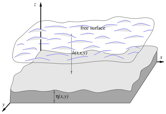
Figure 1. Domain representation.

For the sake of clarity, we specify the following two statements:

(S1)

The boundary portion, where the control action is applied, is given by

$$\begin{array}{c}\hfill {\Gamma }_{{}_1}=\left\{(x,y)\in \partial \Omega :2{\overline{v}}_{{}_1}{n}_x+{\overline{v}}_{{}_2}{n}_y<0\mathrm{and}{\overline{v}}_{{}_1}{n}_x+2{\overline{v}}_{{}_2}{n}_y<0\right\}.\end{array}$$

The boundary portion ${\Gamma }_{{}_1}$ exists (is nonempty) and is included in the boundary portion given by ${({\overline{v}}_{{}_1},{\overline{v}}_{{}_2})}^{\top }·\overrightarrow{\mathbf{n}}<0$, where the vector $\overrightarrow{\mathbf{n}}={(n_x,n_y)}^{\top }$ is the external normal unit vector at the boundary. The uncontrolled boundary portion ${\Gamma }_2=\partial \Omega \backslash {\Gamma }_1$.

(S2)

The flux variation is bounded at the boundary $\partial \Omega$. This follows naturally because of the sub-critical flow regime considered here, and is stated for the sake of clarity. It means that the limit when $(x,y)$ tends to the boundary $\partial \Omega$ of the term ${∥\nabla \mathit{q}∥}_{L^2(\Omega )}$ is bounded, that is,

$$max\left\{\underset{(x,y)\to (x_b,y_b)}{lim}{∥\nabla \mathit{q}(x,y)∥}_{L^2(\Omega )}\mathrm{for}(x_b,y_b)\in \partial \Omega \right\}\mathrm{is}\mathrm{finite}.$$

The regularity of the steady-state $(\overline{h},{\overline{v}}_{{}_1},{\overline{v}}_{{}_2})$ depends on the nature of the bathymetry $\eta$; for instance, $\overline{h}$, ${\overline{v}}_{{}_1}$ and ${\overline{v}}_{{}_2}$ are constant if the bathymetry is constant (flat bottom tomography). We, therefore, consider a sufficiently regular bathymetry $\eta$, such that $\overline{h}$, ${\overline{v}}_{{}_1}$ and ${\overline{v}}_{{}_2}$ are differentiable in $\Omega$: $\overline{h}\in H_0^1(\Omega )$, ${\overline{v}}_{{}_1}\in H^1(\Omega )$ and ${\overline{v}}_{{}_2}\in H^1(\Omega )$.

For $\mathcal{Q}=(0,T)\times \Omega$, we consider the space $L^2\left(0,T;H^1(\Omega )\right)$. In the same setting, we introduce also the space $L^2\left(0,T;H_{{\Gamma }_1}^1(\Omega )\right)$, where the Hilbert space $H_{{\Gamma }_1}^1(\Omega )$ is given by

$$\begin{array}{c}\hfill H_{{\Gamma }_1}^1(\Omega )=\left\{\mathit{u}\in L^2(\Omega ):\nabla \mathit{u}\in L^2(\Omega )\mathrm{and}{\mathit{u}}_{{|}_{{\Gamma }_2}}=0\right\}.\end{array}$$

The space $H^1(\Omega )$ and its subspace $H_{{\Gamma }_1}^1(\Omega )$ are equipped with the norm ${\parallel ·\parallel }_{H^1(\Omega )}$ defined for a function $\mathit{u}$ by ${\parallel \mathit{u}\parallel }_{H^1(\Omega )}^2={\parallel \mathit{u}\parallel }_{L^2(\Omega )}^2+{\parallel \nabla \mathit{u}\parallel }_{L^2(\Omega )}^2$. In the rest of this paper, we denote by W the space given by $W=L^2\left(0,T;H^1(\Omega )\right)\times L^2\left(0,T;H_{{\Gamma }_1}^1(\Omega )\right)\times L^2\left(0,T;H_{{\Gamma }_1}^1(\Omega )\right)$.

3.3. The Stabilization Problem

With the conditions (4), the task of stabilizing the nonlinear state $\left(H,Q_1,Q_{{}_2}\right)$ around the steady state $\left(\overline{h},{\overline{q}}_{{}_1},{\overline{q}}_{{}_2}\right)$ is reformulated as a stabilization problem of the perturbation state $\left(h,\mathit{q}\right)$ around $(0,0,0)$. The objective is to find suitable local boundary conditions on $\mathit{q}$ that take the flow-state variables as quickly as possible to the steady-state equilibrium. We formulate this goal as a stabilization problem in the following way

$$\begin{array}{ccc}\hfill {\partial }_{t}h+\mathrm{div}\mathit{q}& =& 0\mathrm{in}\mathcal{Q},\hfill \\ \hfill {\partial }_t\mathit{q}+\left(\mathrm{div}\mathit{q}\right)\overline{\mathit{v}}+\nabla \mathit{q}·\overline{\mathit{v}}-\mu \Delta \mathit{q}+\mathit{B}·\nabla h+\mathit{A}·\mathit{q}+h{\mathbf{\alpha }}_{{}_0}& =& 0\mathrm{in}\mathcal{Q},\hfill \\ \hfill \mathit{q}(t=0)& =& {\mathit{q}}^0\mathrm{in}\Omega ,\hfill \\ \hfill h(t=0)& =& h^0\mathrm{in}\Omega ,\hfill \\ \hfill \mathit{q}& =& \mathcal{V}\mathrm{on}(0,\infty )\times {\Gamma }_{{}_1},\hfill \\ \hfill \mathit{q}& =& 0\mathrm{on}(0,\infty )\times {\Gamma }_{{}_2}.\hfill \end{array}$$

(6)

Concretely, we look for $\mathcal{V}$ such that $(h,\mathit{q})$ from (6) converges to $(0,0,0)$. In that sequel, we state the weak formulation associated with (6) that consists in writing (6) as a system of ordinary differential equations depending only on the variable t by using the Green’s formula of integration by parts: for all $(\phi ,\varphi ,\psi )\in W$, find $(h,q_{{}_1},q_{{}_2})$ in W satisfying

$$\begin{array}{c}\hfill {\int }_{\Omega }\phi {\partial }_{t}hd\Omega -{\int }_{\Omega }\mathit{q}\nabla \phi d\Omega =-{\int }_{{\Gamma }_{{}_1}}\phi \mathit{q}·\mathbf{n}d\sigma ,\end{array}$$

(7)

$$\begin{array}{ccc}\hfill {\int }_{\Omega }{\partial }_t{q}_{{}_1}\varphi d\Omega & +& {\int }_{\Omega }\left(\mathrm{div}\mathit{q}{\overline{v}}_{{}_1}\right)\varphi d\Omega -{\int }_{\Omega }{q}_{{}_1}\mathrm{div}\left(\varphi \overline{\mathit{v}}\right)d\Omega +\mu {\int }_{\Omega }\nabla q_{{}_1}\nabla \varphi d\Omega -{\int }_{\Omega }h\mathrm{div}\left(\varphi {\mathit{B}}_{{}_{1·}}\right)d\Omega \hfill \\ & +& {\int }_{\Omega }{\beta }_{{}_0}^1{q}_{{}_1}\varphi d\Omega +{\int }_{\Omega }{\gamma }_{{}_0}^1{q}_{{}_2}\varphi d\Omega +{\int }_{\Omega }h{\alpha }_{{}_0}^1\varphi d\Omega \hfill \\ \hfill =& -& {\int }_{{\Gamma }_{{}_1}}\left(q_{{}_1}\varphi \right)\overline{\mathit{v}}·\mathbf{n}d\sigma +\mu {\int }_{{\Gamma }_{{}_1}}(\nabla q_{{}_1}·\mathbf{n})\varphi d\sigma -{\int }_{{\Gamma }_{{}_1}}h\varphi ({\mathit{B}}_{{}_{1·}}·\mathbf{n})d\sigma ,\hfill \end{array}$$

(8)

$$\begin{array}{c}\hfill \\ \hfill {\int }_{\Omega }{\partial }_t{q}_{{}_2}\psi d\Omega & +& {\int }_{\Omega }\left(\mathrm{div}\mathit{q}{\overline{v}}_{{}_2}\right)\psi d\Omega -{\int }_{\Omega }{q}_{{}_2}\mathrm{div}\left(\psi \overline{\mathit{v}}\right)d\Omega +\mu {\int }_{\Omega }\nabla q_{{}_2}\nabla \psi d\Omega -{\int }_{\Omega }h\mathrm{div}\left(\psi {\mathit{B}}_{{}_{2·}}\right)d\Omega \hfill \\ & +& {\int }_{\Omega }{\beta }_{{}_0}^2{q}_{{}_1}\psi d\Omega +{\int }_{\Omega }{\gamma }_{{}_0}^2{q}_{{}_2}\psi d\Omega +{\int }_{\Omega }h{\alpha }_{{}_0}^2\psi d\Omega \hfill \\ \hfill =& -& {\int }_{{\Gamma }_{{}_1}}\left(q_{{}_2}\psi \right)\overline{\mathit{v}}·\mathbf{n}d\sigma +\mu {\int }_{{\Gamma }_{{}_1}}(\nabla q_{{}_2}.n)\psi d\sigma -{\int }_{{\Gamma }_{{}_1}}h\psi ({\mathit{B}}_{{}_{2·}}·\mathbf{n})d\sigma .\hfill \end{array}$$

(9)

From now, the weak formulation of the stabilization problem (6) refers to (7)–(9), which are obtained by integration by parts of (6) multiplied with the test function $(\phi ,\varphi ,\psi )$.

4. Preliminary Result: Small-Time Control Design

The stabilization problem (6) is constrained by the existence of a solution. In this section, we examine the existence of a solution to the dynamical system resulting from the representation of the weak formulation in an Hilbertian basis and we address the short-time stabilization problem.

Lemma 1 (Existence of small-time weak solutions).

There exists a time $T_1$ such that the ordinary differential Equations (7)–(9) with the Cauchy condition admit a solution on the time interval $[0,T_1]$.

The above lemma addresses the existence of local weak solutions. The proof is elaborated in two steps: the first one consists of writing the weak form as a system of differential equations using a Hilbertian basis of finite dimensions of W. The second step deals with the existence of a solution of the resulting system of differential equations thanks to the Cauchy–Peano theorem, see [36,37].

Proof. 

The existence of a local weak solution is elaborated using the Cauchy–Peano theorem. Let ${\left\{a_i\right\}}_{i\ge 1}$ (respectively, by ${\left\{e_i\right\}}_{i\ge 1}$) denote an Hilbertian basis of the space $H^1(\Omega )$ (respectively, $H_{{\Gamma }_1}^1(\Omega )$). We consider a positive integer n such that the finite dimensional space $span\left\{a_i:1\le i\le n\right\}$ contains the term $h_n^0$ of a sequence of functions ${\left(h_n^0\right)}_{n\ge 1}$ that converges toward the initial condition $h^0$ (respectively, $span\left\{e_i:1\le i\le n\right\}$) containing the terms $q_{{}_{1n}}^0$ and $q_{{}_{2n}}^0$ sequences of functions ${\left(q_{{}_{1n}}^0\right)}_{n\ge 1}$ and ${\left(q_{{}_{2n}}^0\right)}_{n\ge 1}$ converging, respectively, to $q_{{}_1}^0$ and $q_{{}_2}^0$). For a sufficiently large n, the projection of h, $q_{{}_1}$ and $q_{{}_2}$ allows us to write

$$\begin{array}{c}\hfill h\approx \sum _{i=1}^n{\alpha }_{{}_i}\left(t\right)a_{{}_i}(x,y),q_{{}_1}\approx \sum _{i=1}^n{\beta }_{{}_i}\left(t\right)e_{{}_i}(x,y),\mathrm{and}{q}_{{}_2}\approx \sum _{i=1}^n{\gamma }_{{}_i}\left(t\right)e_{{}_i}(x,y),\end{array}$$

where ${\left({\alpha }_{{}_i}\left(t\right)\right)}_{1\le i\le n}$, ${\left({\beta }_{{}_i}\left(t\right)\right)}_{1\le i\le n}$ and ${\left({\gamma }_{{}_i}\left(t\right)\right)}_{1\le i\le n}$ are, respectively, the unknown coordinates of h, $q_{{}_1}$ and $q_{{}_2}$ at time t. Replacing test functions $(\phi ,\varphi ,\psi )$ by the $(a_{{}_j},e_{{}_j},e_{{}_j})$ for the $j^{th}$ dimension, the weak formulation becomes:

$$\begin{array}{c}\hfill \sum _{i=1}^n{\partial }_t{\alpha }_{{}_i}\left(t\right){\int }_{\Omega }{a}_{{}_i}{e}_{{}_j}d\Omega -\sum _{i=1}^n{\beta }_{{}_i}\left(t\right){\int }_{\Omega }{a}_{{}_i}{\partial }_x{e}_{{}_j}d\Omega -\sum _{i=1}^n{\gamma }_{{}_i}\left(t\right){\int }_{\Omega }g{a}_{{}_i}{\partial }_y{e}_{{}_j}d\Omega =-{\int }_{{\Gamma }_{{}_1}}{e}_{{}_j}\mathcal{V}·\mathbf{n}d\sigma ,\end{array}$$

$$\begin{array}{ccc}\hfill {\displaystyle \sum _{i=1}^n{\partial }_t{\beta }_{{}_i}\left(t\right){\int }_{\Omega }{e}_{{}_i}{e}_{{}_j}d\Omega }& +& {\displaystyle \sum _{i=1}^n{\beta }_{{}_i}\left(t\right){\int }_{\Omega }{\overline{v}}_{{}_1}{e}_{{}_j}{\partial }_x{e}_{{}_i}d\Omega +\sum _{i=1}^n{\gamma }_{{}_i}\left(t\right){\int }_{\Omega }{\overline{v}}_{{}_1}{e}_{{}_j}{\partial }_y{e}_{{}_i}d\Omega }\hfill \\ & -& {\displaystyle \sum _{i=1}^n{\beta }_{{}_i}\left(t\right){\int }_{\Omega }{e}_{{}_i}\mathrm{div}\left(e_{{}_j}\overline{\mathit{v}}\right)d\Omega +\sum _{i=1}^n{\beta }_{{}_i}\left(t\right)\mu {\int }_{\Omega }\nabla e_{{}_i}\nabla e_{{}_j}d\Omega }\hfill \\ & -& {\displaystyle \sum _{i=1}^n{\alpha }_{{}_i}\left(t\right){\int }_{\Omega }{a}_{{}_i}\mathrm{div}\left(e_{{}_j}{\mathit{B}}_{{}_{1·}}\right)d\Omega +\sum _{i=1}^n{\beta }_{{}_i}\left(t\right){\int }_{\Omega }{\mathit{A}}_{{}_{11}}{e}_{{}_i}{e}_{{}_j}d\Omega }\hfill \\ & +& {\displaystyle \sum _{i=1}^n{\gamma }_{{}_i}\left(t\right){\int }_{\Omega }{\mathit{A}}_{{}_{12}}{e}_{{}_i}{e}_{{}_j}d\Omega +\sum _{i=1}^n{\alpha }_{{}_i}\left(t\right){\int }_{\Omega }{\alpha }_{{}_0}^1{a}_{{}_i}{e}_{{}_j}d\Omega }\hfill \\ & =& {\displaystyle -{\int }_{{\Gamma }_{{}_1}}\left({\mathcal{V}}_{{}_1}{e}_{{}_j}\right)\overline{\mathit{v}}·\mathbf{n}d\sigma +\mu \sum _{i=1}^n{\beta }_{{}_i}\left(t\right){\int }_{{\Gamma }_{{}_1}}(\nabla e_{{}_i}·\mathbf{n})e_{{}_j}d\sigma -{\int }_{{\Gamma }_{{}_1}}h{e}_{{}_j}\left({\mathit{B}}_{{}_{1·}}·\mathbf{n}\right)d\sigma ,}\hfill \end{array}$$

$$\begin{array}{ccc}\hfill {\displaystyle \sum _{i=1}^n{\partial }_t{\gamma }_{{}_i}\left(t\right){\int }_{\Omega }{e}_{{}_i}{e}_{{}_j}d\Omega }& +& {\displaystyle \sum _{i=1}^n{\beta }_{{}_i}\left(t\right){\int }_{\Omega }{\overline{v}}_{{}_2}{e}_{{}_j}{\partial }_x{e}_{{}_i}d\Omega +\sum _{i=1}^n{\gamma }_{{}_i}\left(t\right){\int }_{\Omega }{\overline{v}}_{{}_2}{e}_{{}_j}{\partial }_y{e}_{{}_i}d\Omega }\hfill \\ & -& {\displaystyle \sum _{i=1}^n{\gamma }_{{}_i}\left(t\right){\int }_{\Omega }{e}_{{}_i}\mathrm{div}\left(e_{{}_j}\overline{\mathit{v}}\right)d\Omega +\sum _{i=1}^n{\gamma }_{{}_i}\left(t\right)\mu {\int }_{\Omega }\nabla e_{{}_i}\nabla e_{{}_j}d\Omega }\hfill \\ & -& {\displaystyle \sum _{i=1}^n{\alpha }_{{}_i}\left(t\right){\int }_{\Omega }{a}_{{}_i}\mathrm{div}\left(e_{{}_j}{\mathit{B}}_{{}_{2·}}\right)d\Omega +\sum _{i=1}^n{\beta }_{{}_i}\left(t\right){\int }_{\Omega }{\mathit{A}}_{{}_{21}}{e}_{{}_i}{e}_{{}_j}d\Omega }\hfill \\ & +& {\displaystyle \sum _{i=1}^n{\gamma }_{{}_i}\left(t\right){\int }_{\Omega }{\mathit{A}}_{{}_{22}}{e}_{{}_i}{e}_{{}_j}d\Omega +\sum _{i=1}^n{\alpha }_{{}_i}\left(t\right){\int }_{\Omega }{\alpha }_0^2{a}_{{}_i}{e}_{{}_j}d\Omega }\hfill \\ & =& {\displaystyle -{\int }_{{\Gamma }_{{}_1}}\left({\mathcal{V}}_{{}_2}{e}_{{}_j}\right)\overline{\mathit{v}}·\mathbf{n}d\sigma +\mu \sum _{i=1}^n{\gamma }_{{}_i}\left(t\right){\int }_{{\Gamma }_{{}_1}}(\nabla e_{{}_i}·\mathbf{n})e_{{}_j}d\sigma -{\int }_{{\Gamma }_{{}_1}}h{e}_{{}_j}\left({\mathit{B}}_{{}_{2·}}·\mathbf{n}\right)d\sigma .}\hfill \end{array}$$

Let us introduce the matrices ${\mathit{M}}_k$ for $k=1,\cdots ,11$ as well as the vectors ${\mathit{m}}_l$ for $l=1,\cdots ,3$ as follows

$$\begin{array}{ccc}\hfill {\mathit{M}}_{1_{ji}}& =& {\int }_{\Omega }{a}_{{}_i}{e}_{{}_j}d\Omega ,{\mathit{M}}_{2_{ji}}={\int }_{\Omega }{a}_{{}_i}{\partial }_x{e}_{{}_j}d\Omega ,{\mathit{M}}_{3_{ji}}={\int }_{\Omega }{a}_{{}_i}{\partial }_y{e}_{{}_j}d\Omega \hfill \\ \hfill {\mathit{M}}_{4_{ji}}& =& {\int }_{\Omega }{e}_{{}_i}{e}_{{}_j}d\Omega ,{\mathit{M}}_{5_{ji}}={\int }_{\Omega }{\overline{v}}_{{}_1}{e}_{{}_j}{\partial }_x{e}_{{}_i}d\Omega -{\int }_{\Omega }{e}_{{}_i}\mathrm{div}\left(e_{{}_j}\overline{\mathit{v}}\right)d\Omega +\mu {\int }_{\Omega }\nabla e_{{}_i}\nabla e_{{}_j}d\Omega +{\int }_{\Omega }{\mathit{A}}_{{}_{11}}{e}_{{}_i}{e}_{{}_j}d\Omega ,\hfill \\ \hfill {\mathit{M}}_{6_{ji}}& =& {\int }_{\Omega }{\overline{v}}_{{}_1}{e}_{{}_j}{\partial }_y{e}_{{}_i}d\Omega +{\int }_{\Omega }{\mathit{A}}_{{}_{12}}{e}_{{}_i}{e}_{{}_j}d\Omega ,{\mathit{M}}_{7_{ji}}=-{\int }_{\Omega }{e}_{{}_i}\mathrm{div}\left(e_{{}_j}{\mathit{B}}_{{}_{1·}}\right)d\Omega +{\int }_{\Omega }{\alpha }_{{}_0}^1{e}_{{}_i}{e}_{{}_j}d\Omega ,\hfill \end{array}$$

$$\begin{array}{ccc}\hfill {\mathit{M}}_{8_{ji}}& =& {\int }_{\Omega }{\overline{v}}_{{}_2}{e}_{{}_j}{\partial }_x{e}_{{}_i}d\Omega +{\int }_{\Omega }{\mathit{A}}_{{}_{21}}{e}_{{}_i}{e}_{{}_j}d\Omega ,\hfill \\ \hfill {\mathit{M}}_{9_{ji}}& =& {\int }_{\Omega }{\overline{v}}_{{}_2}{e}_{{}_j}{\partial }_y{e}_{{}_i}d\Omega -{\int }_{\Omega }{e}_{{}_i}\mathrm{div}\left(e_{{}_j}\overline{\mathit{v}}\right)d\Omega +\mu {\int }_{\Omega }\nabla e_{{}_i}\nabla e_{{}_j}d\Omega +{\int }_{\Omega }{\mathit{A}}_{{}_{22}}{e}_{{}_i}{e}_{{}_j}d\Omega \hfill \\ \hfill {\mathit{M}}_{{10}_{ji}}& =& -{\int }_{\Omega }{e}_{{}_i}\mathrm{div}\left(e_{{}_j}{\mathit{B}}_{{}_{2·}}\right)d\Omega +{\int }_{\Omega }{\alpha }_{{}_0}^2{e}_{{}_i}{e}_{{}_j}d\Omega ,{\mathit{M}}_{{11}_{ji}}=\mu {\int }_{{\Gamma }_{{}_1}}(\nabla e_{{}_i}·\mathbf{n})e_{{}_j}d\sigma ,\hfill \end{array}$$

and

$$\begin{array}{ccc}\hfill {\mathit{m}}_{1_j}& =& -{\int }_{{\Gamma }_{{}_1}}{e}_{{}_j}{n}_{x}d\sigma ,{\mathit{m}}_{2_j}=-{\int }_{{\Gamma }_1}{e}_{{}_j}{n}_{y}d\sigma ,{\mathit{m}}_{3_j}=-{\int }_{{\Gamma }_{{}_1}}{e}_{{}_j}\overline{\mathit{v}}·\mathbf{n}d\sigma ,\hfill \\ \hfill {\mathit{m}}_{4_j}& =& -{\int }_{{\Gamma }_{{}_1}}h{e}_{{}_j}\left({\mathit{B}}_{{}_{1·}}·\mathbf{n}\right)d\sigma {\mathit{m}}_{5_j}=-{\int }_{{\Gamma }_{{}_1}}h{e}_{{}_j}\left({\mathit{B}}_{{}_{2·}}·\mathbf{n}\right)d\sigma .\hfill \end{array}$$

We now count the n components; this yields the following system of matrix equations

$$\begin{array}{c}\hfill \left\{\begin{array}{c}{\displaystyle {\mathit{M}}_1{\partial }_t\mathit{a}\left(t\right)-{\mathit{M}}_2\mathit{b}\left(t\right)-{\mathit{M}}_3\mathit{c}\left(t\right)={\mathcal{V}}_{{}_1}{\mathit{m}}_1+{\mathcal{V}}_{{}_2}{\mathit{m}}_2,}\hfill \\ \\ {\displaystyle {\mathit{M}}_4{\partial }_t\mathit{b}\left(t\right)+{\mathit{M}}_5\mathit{b}\left(t\right)+{\mathit{M}}_6\mathit{c}\left(t\right)+{\mathit{M}}_7\mathit{a}\left(t\right)={\mathcal{V}}_{{}_1}{\mathit{m}}_3+{\mathit{M}}_{11}\mathit{b}\left(t\right)+{\mathit{m}}_4,}\hfill \\ \\ {\displaystyle {\mathit{M}}_4{\partial }_t\mathit{c}\left(t\right)+{\mathit{M}}_8\mathit{b}\left(t\right)+{\mathit{M}}_9\mathit{c}\left(t\right)+{\mathit{M}}_{10}\mathit{a}\left(t\right)={\mathcal{V}}_{{}_2}{\mathit{m}}_3+{\mathit{M}}_{11}\mathit{c}\left(t\right)+{\mathit{m}}_5,}\hfill \end{array}\right.\end{array}$$

where the vectors $\mathit{a}$, $\mathit{b}$ and $\mathit{c}$ are given by the coordinates of the state variables h, $q_{{}_1}$ and $q_{{}_2}$, respectively, i.e., $\mathit{a}=({\alpha }_{{}_1},\cdots ,{\alpha }_{{}_n})$, $\mathit{b}=({\beta }_{{}_1},\cdots ,{\beta }_{{}_n})$, and $\mathit{c}=({\gamma }_{{}_1},\cdots ,{\gamma }_{{}_n})$. To introduce the matrices:

$$\begin{array}{c}\hfill {\mathit{P}}_1=\left(\begin{array}{ccc}{\displaystyle {\mathit{M}}_1}& {\displaystyle 0}& {\displaystyle 0}\\ {\displaystyle 0}& {\displaystyle {\mathit{M}}_4}& {\displaystyle 0}\\ {\displaystyle 0}& {\displaystyle 0}& {\displaystyle {\mathit{M}}_4}\end{array}\right),{\mathit{P}}_2=\left(\begin{array}{ccc}{\displaystyle 0}& {\displaystyle {\mathit{M}}_2}& {\displaystyle {\mathit{M}}_3}\\ {\displaystyle {\mathit{M}}_7}& {\displaystyle {\mathit{M}}_5}& {\displaystyle {\mathit{M}}_6}\\ {\displaystyle {\mathit{M}}_{10}}& {\displaystyle {\mathit{M}}_8}& {\displaystyle {\mathit{M}}_9}\end{array}\right),\mathrm{and}{\mathit{P}}_3=\left(\begin{array}{ccc}{\displaystyle 0}& {\displaystyle 0}& {\displaystyle 0}\\ {\displaystyle 0}& {\displaystyle {\mathit{M}}_{11}}& {\displaystyle 0}\\ {\displaystyle 0}& {\displaystyle 0}& {\displaystyle {\mathit{M}}_{11}}\end{array}\right),\end{array}$$

and the vectors

$$\begin{array}{c}\hfill \mathit{y}=\left(\begin{array}{c}{\displaystyle \mathit{a}}\\ {\displaystyle \mathit{b}}\\ {\displaystyle \mathit{c}}\end{array}\right),{\mathit{p}}_1=\left(\begin{array}{c}{\displaystyle {\mathit{m}}_1}\\ {\displaystyle {\mathit{m}}_3}\\ {\displaystyle 0}\end{array}\right),{\mathit{p}}_2=\left(\begin{array}{c}{\displaystyle {\mathit{m}}_2}\\ {\displaystyle 0}\\ {\displaystyle {\mathit{m}}_3}\end{array}\right)\mathrm{and}{\mathit{p}}_3=\left(\begin{array}{c}{\displaystyle 0}\\ {\displaystyle {\mathit{m}}_4}\\ {\displaystyle {\mathit{m}}_5}\end{array}\right),\end{array}$$

we write the weak form of Equations (7)–(9) together as an ordinary differential equation, with the initial condition ${\mathit{y}}_0$ associated with $(h^0,{\mathit{q}}^0)$, in the form

$$\begin{array}{c}\hfill \left\{\begin{array}{c}{\displaystyle {\mathit{y}}^{\prime }\left(t\right)=\mathit{f}(t,\mathit{y}),}\hfill \\ {\displaystyle \mathit{y}(t=0)={\mathit{y}}_0,}\hfill \end{array}\right.\end{array}$$

(10)

where

$$\begin{array}{c}\hfill {\displaystyle \mathit{f}(t,\mathit{y}\left(t\right))=-{\mathit{P}}_1^{-1}{\mathit{P}}_2\mathit{y}\left(t\right)+{\mathit{P}}_1^{-1}{\mathit{P}}_3\mathit{y}\left(t\right)+{\mathcal{V}}_{{}_1}\left(t\right){\mathit{P}}_1^{-1}{\mathit{p}}_1+{\mathcal{V}}_{{}_2}\left(t\right){\mathit{P}}_1^{-1}{\mathit{p}}_2+{\mathit{P}}_1^{-1}{\mathit{p}}_3\left(t\right).}\end{array}$$

It remains now to prove the continuity of the functional $\mathit{f}$. For that, we consider the matrix norm ${∥·∥}_2$ given by:

$$\begin{array}{c}\hfill {\displaystyle {∥\mathit{M}∥}_2=\underset{\mathbf{\zeta }}{sup}\frac{{∥\mathit{M}\mathbf{\zeta }∥}_2}{{∥\mathbf{\zeta }∥}_2},\mathrm{where}{∥\mathbf{\zeta }∥}_2=\sqrt{\sum _i^n{\left|{\mathbf{\zeta }}_i\right|}^2}.}\end{array}$$

We have

$$\begin{array}{ccc}\hfill {∥\mathit{f}∥}_2& =& {∥-{\mathit{P}}_1^{-1}{\mathit{P}}_2\mathit{y}\left(t\right)+{\mathit{P}}_1^{-1}{\mathit{P}}_3\mathit{y}\left(t\right)+{\mathcal{V}}_{{}_1}\left(t\right){\mathit{P}}_1^{-1}{\mathit{p}}_1+{\mathcal{V}}_{{}_2}\left(t\right){\mathit{P}}_1^{-1}{\mathit{p}}_2+{\mathit{P}}_1^{-1}{\mathit{p}}_3\left(t\right)∥}_2\hfill \\ & \le & {∥-{\mathit{P}}_1^{-1}{\mathit{P}}_2\mathit{y}\left(t\right)∥}_2+{∥{\mathit{P}}_1^{-1}{\mathit{P}}_3\mathit{y}\left(t\right)∥}_2+{∥{\mathcal{V}}_{{}_1}\left(t\right){\mathit{P}}_1^{-1}{\mathit{p}}_1∥}_2+{∥{\mathcal{V}}_{{}_2}\left(t\right){\mathit{P}}_1^{-1}{\mathit{p}}_2∥}_2+{∥{\mathit{P}}_1^{-1}{\mathit{p}}_3\left(t\right)∥}_2.\hfill \end{array}$$

Yet, we know that

$$\begin{array}{ccc}\hfill {∥-{\mathit{P}}_1^{-1}{\mathit{P}}_2\mathit{y}∥}_2& =& {∥-{\mathit{P}}_1^{-1}{\mathit{P}}_2\left(\mathit{y}-{\mathit{y}}_0+{\mathit{y}}_0\right)∥}_2\hfill \\ & \le & {∥-{\mathit{P}}_1^{-1}{\mathit{P}}_2\left(\mathit{y}-{\mathit{y}}_0\right)∥}_2+{∥-{\mathit{P}}_1^{-1}{\mathit{P}}_2{\mathit{y}}_0∥}_2\hfill \\ & \le & {∥-{\mathit{P}}_1^{-1}{\mathit{P}}_2∥}_2\left({∥\mathit{y}-{\mathit{y}}_0∥}_2+{∥{\mathit{y}}_0∥}_2\right).\hfill \end{array}$$

Similarly, we bound the quantity ${∥-{\mathit{P}}_1^{-1}{\mathit{P}}_3\mathit{y}∥}_2$. The terms ${∥{\mathcal{V}}_{{}_1}\left(t\right){\mathit{P}}_1^{-1}{\mathit{p}}_1∥}_2$ and ${∥{\mathcal{V}}_{{}_2}\left(t\right){\mathit{P}}_1^{-1}{\mathit{p}}_2∥}_2$ contain the control actions $({\mathcal{V}}_{{}_1},{\mathcal{V}}_{{}_2})$; their majoration follows from the statement (S2). As the perturbation state for the height is supposed to be small compared to $\overline{h}$ and given the definition of the space W, the term ${∥{\mathit{P}}_1^{-1}{\mathit{p}}_3\left(t\right)∥}_2$ is bounded. Therefore, there exists a constant $K_{{}_1}$ such that

$$\begin{array}{c}\hfill {∥\mathit{f}∥}_2\le K_{{}_1}.\end{array}$$

(11)

It is clear that ${∥\mathit{y}-{\mathit{y}}_0∥}_2\le E\left(0\right)$ because the control law acts to decrease the initial total energy $E\left(0\right)$. Denoting $T_{{}_1}=E\left(0\right)/K_{{}_1}$, it yields that $\mathit{f}$ is bounded according to (11). Moreover, $\mathit{f}$ is continuous because it is a composition of a linear function followed by a translation. Therefore, the Cauchy–Peano theorem ensures the existence of solutions to (10) in the time interval $[0,T_{{}_1}]$. □

The proof below is enough for the infinite dimensional setting in Lemma 1 because for the drift function $\mathit{f}$ satisfying the Lipschitz condition in the variable $\mathit{y}$, the Cauchy–Picard theorem, see [38], transmits the result from the finite dimensional case to an infinite dimensional case. Yet, the drift $\mathit{f}$ fulfills the Lipschitz condition because of (11) and its affine structure.

4.1. Energy Estimate

Here, we define and estimate the energy of the perturbation state at a time $t\in [0,T_1]$.

Definition 1 (Energy).

For $t\in [0,T_{{}_1}]$, we consider the energy defined as:

$$\begin{array}{ccc}\hfill E\left(t\right)& =& {∥\sqrt{g\overline{h}}h∥}_{L^2(\Omega )}^2+{∥q_{{}_1}∥}_{L^2(\Omega )}^2+{∥q_{{}_2}∥}_{L^2(\Omega )}^2+\mu {\int }_0^t{∥\nabla \mathit{q}\left(\tau \right)∥}_{L^2(\Omega )}^{2}d\tau \hfill \\ & =& E^1\left(t\right)+\mu {\int }_0^t{∥\nabla \mathit{q}\left(\tau \right)∥}_{L^2(\Omega )}^{2}d\tau ,\hfill \end{array}$$

(12)

where $E^1\left(t\right)$ is the non-viscous energy and $T_{{}_1}$ is the time bound given in Lemma 1.

To establish an estimate on the energy, we replace the test functions $(\phi ,\varphi ,\psi )$ by $(g\overline{h}h,\mathit{q})$ in the variational form (7)–(9), to obtain

$$\begin{array}{c}\hfill {\displaystyle \frac{1}{2}{\int }_{\Omega }g\overline{h}{\partial }_t{h}^{2}d\Omega -{\int }_{\Omega }g\mathit{q}·\nabla \left(\overline{h}h\right)d\Omega =-{\int }_{{\Gamma }_{{}_1}}g\overline{h}h\mathit{q}·\mathbf{n}d\sigma ,}\end{array}$$

$$\begin{array}{ccc}\hfill {\displaystyle \frac{1}{2}{\int }_{\Omega }{\partial }_t\left(q_{{}_1}^2+q_{{}_2}^2\right)d\Omega }& +& {\displaystyle \mu {\int }_{\Omega }{∥\nabla \mathit{q}∥}_2^{2}d\Omega +{\int }_{\Omega }\left(\mathrm{div}\mathit{q}\right)\overline{\mathit{v}}·\mathit{q}d\Omega -{\int }_{\Omega }{q}_{{}_1}\mathrm{div}\left(q_{{}_1}\overline{\mathit{v}}\right)d\Omega }\hfill \\ & -& {\displaystyle {\int }_{\Omega }{q}_{{}_2}\mathrm{div}\left(q_{{}_2}\overline{\mathit{v}}\right)d\Omega -{\int }_{\Omega }h\mathrm{div}(\mathit{B}·\mathit{q})d\Omega +{\int }_{\Omega }(\mathit{A}·\mathit{q})·\mathit{q}d\Omega +{\int }_{\Omega }h{\mathbf{\alpha }}_{{}_0}·\mathit{q}d\Omega }\hfill \\ & =& {\displaystyle -{\int }_{{\Gamma }_{{}_1}}(q_{{}_1}^2+q_{{}_2}^2)\overline{\mathit{v}}·\mathbf{n}d\sigma +\mu {\int }_{{\Gamma }_{{}_1}}(q_{{}_1}\nabla q_{{}_1}+q_{{}_2}\nabla q_{{}_2})·\mathbf{n}d\sigma -{\int }_{{\Gamma }_{{}_1}}h(\mathit{B}·\mathit{q})·\mathbf{n}d\sigma .}\hfill \end{array}$$

Adding the two equalities yields

$$\begin{array}{ccc}\hfill {\displaystyle \frac{1}{2}{\partial }_t{E}^1\left(t\right)+\mu {\int }_{\Omega }{∥\nabla \mathit{q}∥}_2^{2}d\Omega }& =& {\displaystyle I_{{}_1}+I_{{}_2}+I_{{}_3}+I_{{}_4}-{\int }_{{\Gamma }_{{}_1}}g\overline{h}h\mathit{q}·\mathbf{n}d\sigma -{\int }_{{\Gamma }_{{}_1}}(q_{{}_1}^2+q_{{}_2}^2)\overline{\mathit{v}}·\mathbf{n}d\sigma }\hfill \\ & & {\displaystyle +\mu {\int }_{{\Gamma }_{{}_1}}(q_{{}_1}\nabla q_{{}_1}+q_{{}_2}\nabla q_{{}_2})·\mathbf{n}d\sigma -{\int }_{{\Gamma }_{{}_1}}h(\mathit{B}·\mathit{q})·\mathbf{n}d\sigma ,}\hfill \end{array}$$

where the quantities $I_{{}_i}$ are given by

$$\begin{array}{ccccc}\hfill & I_{{}_1}={\int }_{\Omega }g\mathit{q}·\nabla \left(\overline{h}h\right)d\Omega +{\int }_{\Omega }h\mathrm{div}(\mathit{B}·\mathit{q})d\Omega ,\hfill & \hfill & I_{{}_2}=-{\int }_{\Omega }\mathrm{div}\mathit{q}\overline{\mathit{v}}·\mathit{q}d\Omega ,\hfill & \\ \hfill & I_{{}_3}={\int }_{\Omega }{q}_{{}_1}\mathrm{div}\left(q_{{}_1}\overline{\mathit{v}}\right)d\Omega +{\int }_{\Omega }{q}_{{}_2}\mathrm{div}\left(q_{{}_2}\overline{\mathit{v}}\right)d\Omega ,\hfill & \hfill & I_{{}_4}=-{\int }_{\Omega }(\mathit{A}·\mathit{q})·\mathit{q}d\Omega -{\int }_{\Omega }h{\mathbf{\alpha }}_{{}_0}·\mathit{q}d\Omega .\hfill \end{array}$$

We now investigate how to isolate the nonlinear terms in each $I_{{}_i}$ with the purpose of having no derivative terms on the boundary. For that, we apply the Green formula in an adaptive manner. Afterward, we take the maximum bound over the steady-state variables, which allows us to obtain a bound estimate for each quantity. For the quantity $I_{{}_1}$, it comes that

$$\begin{array}{ccc}\hfill {\displaystyle I_{{}_1}}& \le & {\displaystyle \underset{\Omega }{max}\left(\frac{g∥\nabla \overline{h}∥}{\sqrt{\overline{h}}}\right){\int }_{\Omega }\sqrt{\overline{h}}∥h\mathit{q}∥d\Omega +\underset{\Omega }{max}\left(\frac{{\overline{v}}_{{}_1}^2}{\sqrt{\overline{h}}}\right){\int }_{\Omega }\sqrt{\overline{h}}\left|h{\partial }_x{q}_{{}_1}\right|d\Omega }\hfill \\ & & {\displaystyle +\underset{\Omega }{max}\left(\frac{\left|{\partial }_x{\overline{v}}_{{}_1}^2\right|}{\sqrt{\overline{h}}}\right){\int }_{\Omega }\sqrt{\overline{h}}\left|h{q}_{{}_1}\right|d\Omega +\underset{\Omega }{max}\left(\frac{{\overline{v}}_{{}_2}^2}{\sqrt{\overline{h}}}\right){\int }_{\Omega }\sqrt{\overline{h}}\left|h{\partial }_y{q}_{{}_2}\right|d\Omega }\hfill \\ & & {\displaystyle +\underset{\Omega }{max}\left(\frac{\left|{\partial }_y{\overline{v}}_{{}_2}^2\right|}{\sqrt{\overline{h}}}\right){\int }_{\Omega }\sqrt{\overline{h}}\left|h{q}_{{}_2}\right|d\Omega +\underset{\Omega }{max}\left(\frac{\left|{\overline{v}}_{{}_1}{\overline{v}}_{{}_2}\right|}{\sqrt{\overline{h}}}\right){\int }_{\Omega }\sqrt{\overline{h}}\left|h{\partial }_x{q}_{{}_2}\right|d\Omega }\hfill \\ & & {\displaystyle +\underset{\Omega }{max}\left(\frac{\left|{\partial }_x\left({\overline{v}}_{{}_1}{\overline{v}}_{{}_2}\right)\right|}{\sqrt{\overline{h}}}\right){\int }_{\Omega }\sqrt{\overline{h}}\left|h{q}_{{}_2}\right|d\Omega +\underset{\Omega }{max}\left(\frac{\left|{\overline{v}}_{{}_1}{\overline{v}}_{{}_2}\right|}{\sqrt{\overline{h}}}\right){\int }_{\Omega }\sqrt{\overline{h}}\left|h{\partial }_y{q}_{{}_1}\right|d\Omega }\hfill \\ \hfill & & {\displaystyle +\underset{\Omega }{max}\left(\frac{\left|{\partial }_y\left({\overline{v}}_{{}_1}{\overline{v}}_{{}_2}\right)\right|}{\sqrt{\overline{h}}}\right){\int }_{\Omega }\sqrt{\overline{h}}\left|h{q}_{{}_1}\right|d\Omega +{\int }_{\partial \Omega }g\overline{h}h\mathit{q}·\mathbf{n}d\sigma .}\hfill \end{array}$$

(13)

Similarly, we bound the quantities $I_{{}_2}$, $I_{{}_3}$, and $I_{{}_4}$ as follows

$$\begin{array}{ccc}\hfill {\displaystyle I_{{}_2}}& \le & {\displaystyle \frac{1}{2}\underset{\Omega }{max}\left(\left|{\partial }_x{\overline{v}}_{{}_1}\right|\right){\int }_{\Omega }{q}_{{}_1}^{2}d\Omega +\frac{1}{2}\underset{\Omega }{max}\left(\left|{\partial }_y{\overline{v}}_{{}_2}\right|\right){\int }_{\Omega }{q}_{{}_2}^{2}d\Omega +\underset{\Omega }{max}\left(\left|{\overline{v}}_{{}_1}\right|\right){\int }_{\Omega }\left|q_{{}_1}{\partial }_y{q}_{{}_2}\right|d\Omega }\hfill \\ \hfill & & {\displaystyle +\underset{\Omega }{max}\left(\left|{\overline{v}}_{{}_2}\right|\right){\int }_{\Omega }\left|q_{{}_2}{\partial }_x{q}_{{}_1}\right|d\Omega -{\int }_{\partial \Omega }\frac{{\overline{v}}_{{}_1}}{2}{q}_{{}_1}^2{n}_{x}d\sigma -{\int }_{\partial \Omega }\frac{{\overline{v}}_{{}_2}}{2}{q}_{{}_2}^2{n}_{y}d\sigma ,}\hfill \end{array}$$

(14)

$$\begin{array}{ccc}\hfill {\displaystyle I_{{}_3}}& \le & {\displaystyle \frac{1}{2}\underset{\Omega }{max}\left(\left|{\partial }_x{\overline{v}}_{{}_1}\right|\right){\int }_{\Omega }{q}_{{}_1}^{2}d\Omega +\underset{\Omega }{max}\left(\left|{\partial }_x{\overline{v}}_{{}_2}\right|\right){\int }_{\Omega }\left|q_{{}_1}{q}_{{}_2}\right|d\Omega +\underset{\Omega }{max}\left(\left|{\overline{v}}_{{}_2}\right|\right){\int }_{\Omega }\left|q_{{}_1}{\partial }_x{q}_{{}_2}\right|d\Omega }\hfill \\ & & {\displaystyle +\underset{\Omega }{max}\left(\left|{\partial }_y{\overline{v}}_{{}_2}\right|\right){\int }_{\Omega }\left|q_{{}_1}{q}_{{}_2}\right|d\Omega +\underset{\Omega }{max}\left(\left|{\overline{v}}_{{}_1}\right|\right){\int }_{\Omega }\left|q_{{}_2}{\partial }_y{q}_{{}_1}\right|d\Omega +\frac{1}{2}\underset{\Omega }{max}\left(\left|{\partial }_y{\overline{v}}_{{}_2}\right|\right){\int }_{\Omega }{q}_{{}_2}^{2}d\Omega }\hfill \\ \hfill & & {\displaystyle -{\int }_{\partial \Omega }\frac{{\overline{v}}_{{}_1}}{2}{q}_{{}_1}^2{n}_{x}d\sigma -{\int }_{\partial \Omega }\frac{{\overline{v}}_{{}_2}}{2}{q}_{{}_2}^2{n}_{y}d\sigma ,}\hfill \end{array}$$

(15)

and

$$\begin{array}{ccc}\hfill {\displaystyle I_{{}_4}}& \le & {\displaystyle \underset{\Omega }{max}\left(\left|{\beta }_{{}_0}^1\right|\right){\int }_{\Omega }{q}_{{}_1}^{2}d\Omega +\underset{\Omega }{max}\left(\left|{\gamma }_{{}_0}^1+{\beta }_{{}_0}^2\right|\right){\int }_{\Omega }\left|q_{{}_1}{q}_{{}_2}\right|d\Omega +\underset{\Omega }{max}\left(\left|{\gamma }_{{}_0}^2\right|\right){\int }_{\Omega }{q}_{{}_2}^{2}d\Omega }\hfill \\ \hfill & & {\displaystyle +\underset{\Omega }{max}\left(\frac{\left|{\alpha }_{{}_0}^1\right|}{\sqrt{\overline{h}}}\right){\int }_{\Omega }\sqrt{\overline{h}}\left|h{q}_{{}_1}\right|d\Omega +\underset{\Omega }{max}\left(\frac{\left|{\alpha }_{{}_0}^2\right|}{\sqrt{\overline{h}}}\right){\int }_{\Omega }\sqrt{\overline{h}}\left|h{q}_{{}_2}\right|d\Omega .}\hfill \end{array}$$

(16)

We now apply the Young inequality to separate the nonlinear terms (in the perturbation state) for the upper bound of each of the inequalities (13)–(16). That implies the existence of ${\epsilon }_i$ for $(i=1,\cdots ,18)$, such that

$$\begin{array}{ccc}\hfill {\displaystyle \frac{1}{2}{\partial }_t{E}^1\left(t\right)+\mu {\int }_{\Omega }{∥\nabla \mathit{q}∥}_2^{2}d\Omega }& \le & {\displaystyle T_{{}_{\mathrm{bord}}}\left(t\right)+C_{{}_h}{\int }_{\Omega }\overline{h}{h}^{2}d\Omega +C_{q_1}{\int }_{\Omega }{q}_{{}_1}^{2}d\Omega +C_{q_2}{\int }_{\Omega }{q}_{{}_2}^{2}d\Omega }\hfill \\ & & {\displaystyle +\left({\epsilon }_2\underset{\Omega }{max}\left(\frac{{\overline{v}}_{{}_1}^2}{\sqrt{\overline{h}}}\right)+{\epsilon }_{11}\underset{\Omega }{max}\left(\left|{\overline{v}}_2\right|\right)\right){\int }_{\Omega }{\left({\partial }_x{q}_{{}_1}\right)}^{2}d\Omega }\hfill \\ & & {\displaystyle +\left({\epsilon }_8\underset{\Omega }{max}\left(\frac{\left|{\overline{v}}_{{}_1}{\overline{v}}_{{}_2}\right|}{\sqrt{\overline{h}}}\right)+{\epsilon }_{15}\underset{\Omega }{max}\left(\left|{\overline{v}}_{{}_1}\right|\right)\right){\int }_{\Omega }{\left({\partial }_y{q}_{{}_1}\right)}^{2}d\Omega }\hfill \\ & & {\displaystyle +\left({\epsilon }_6\underset{\Omega }{max}\left(\frac{\left|{\overline{v}}_{{}_1}{\overline{v}}_{{}_2}\right|}{\sqrt{\overline{h}}}\right)+{\epsilon }_{13}\underset{\Omega }{max}\left(\left|{\overline{v}}_{{}_2}\right|\right)\right){\int }_{\Omega }{\left({\partial }_x{q}_{{}_2}\right)}^{2}d\Omega }\hfill \\ & & {\displaystyle +\left({\epsilon }_4\underset{\Omega }{max}\left(\frac{{\overline{v}}_{{}_2}^2}{\sqrt{\overline{h}}}\right)+{\epsilon }_{10}\underset{\Omega }{max}\left(\left|{\overline{v}}_{{}_1}\right|\right)\right){\int }_{\Omega }{\left({\partial }_y{q}_{{}_2}\right)}^{2}d\Omega ,}\hfill \end{array}$$

where

$$\begin{array}{ccc}\hfill {\displaystyle C_{{}_h}}& =& {\displaystyle \frac{1}{{\epsilon }_1}\underset{\Omega }{max}\left(\frac{g∥\nabla \overline{h}∥}{\sqrt{\overline{h}}}\right)+\frac{1}{{\epsilon }_2}\underset{\Omega }{max}\left(\frac{{\overline{v}}_{{}_1}^2}{\sqrt{\overline{h}}}\right)+\frac{1}{{\epsilon }_3}\underset{\Omega }{max}\left(\frac{\left|{\partial }_x{\overline{v}}_{{}_1}^2\right|}{\sqrt{\overline{h}}}\right)+\frac{1}{{\epsilon }_4}\underset{\Omega }{max}\left(\frac{{\overline{v}}_{{}_2}^2}{\sqrt{\overline{h}}}\right);}\hfill \\ & & {\displaystyle +\frac{1}{{\epsilon }_5}\underset{\Omega }{max}\left(\frac{\left|{\partial }_y{\overline{v}}_{{}_2}^2\right|}{\sqrt{\overline{h}}}\right)+\frac{1}{{\epsilon }_6}\underset{\Omega }{max}\left(\frac{\left|{\overline{v}}_{{}_1}{\overline{v}}_{{}_2}\right|}{\sqrt{\overline{h}}}\right)+\frac{1}{{\epsilon }_7}\underset{\Omega }{max}\left(\frac{\left|{\partial }_x\left({\overline{v}}_{{}_1}{\overline{v}}_{{}_2}\right)\right|}{\sqrt{\overline{h}}}\right)+\frac{1}{{\epsilon }_8}\underset{\Omega }{max}\left(\frac{\left|{\overline{v}}_{{}_1}{\overline{v}}_{{}_2}\right|}{\sqrt{\overline{h}}}\right)}\hfill \\ & & {\displaystyle +\frac{1}{{\epsilon }_9}\underset{\Omega }{max}\left(\frac{\left|{\partial }_y\left({\overline{v}}_{{}_1}{\overline{v}}_{{}_2}\right)\right|}{\sqrt{\overline{h}}}\right)+\frac{1}{{\epsilon }_{17}}\underset{\Omega }{max}\left(\frac{\left|{\alpha }_{{}_0}^1\right|}{\sqrt{\overline{h}}}\right)+\frac{1}{{\epsilon }_{18}}\underset{\Omega }{max}\left(\frac{\left|{\alpha }_{{}_0}^2\right|}{\sqrt{\overline{h}}}\right),}\hfill \end{array}$$

$$\begin{array}{ccc}\hfill {\displaystyle C_{q_1}}& =& {\displaystyle {\epsilon }_1\underset{\Omega }{max}\left(\frac{g∥\nabla \overline{h}∥}{\sqrt{\overline{h}}}\right)+{\epsilon }_3\underset{\Omega }{max}\left(\frac{\left|{\partial }_x{\overline{v}}_{{}_1}^2\right|}{\sqrt{\overline{h}}}\right)+{\epsilon }_9\underset{\Omega }{max}\left(\frac{\left|{\partial }_y\left({\overline{v}}_{{}_1}{\overline{v}}_{{}_2}\right)\right|}{\sqrt{\overline{h}}}\right)+\underset{\Omega }{max}\left(\left|{\partial }_x{\overline{v}}_{{}_1}\right|\right)}\hfill \\ & & {\displaystyle +\frac{1}{{\epsilon }_{10}}\underset{\Omega }{max}\left(\left|{\overline{v}}_{{}_1}\right|\right)+\frac{1}{{\epsilon }_{12}}\underset{\Omega }{max}\left(\left|{\partial }_x{\overline{v}}_{{}_2}\right|\right)+\frac{1}{{\epsilon }_{13}}\underset{\Omega }{max}\left(\left|{\overline{v}}_{{}_2}\right|\right)+\frac{1}{{\epsilon }_{14}}\underset{\Omega }{max}\left(\left|{\partial }_y{\overline{v}}_{{}_1}\right|\right)+\underset{\Omega }{max}\left({\beta }_{{}_0}^1\right)}\hfill \\ & & {\displaystyle +\frac{1}{{\epsilon }_{16}}\underset{\Omega }{max}\left(\left|{\gamma }_{{}_0}^1+{\beta }_{{}_0}^2\right|\right)+{\epsilon }_{17}\underset{\Omega }{max}\left(\frac{\left|{\alpha }_{{}_0}^1\right|}{\sqrt{\overline{h}}}\right),}\hfill \end{array}$$

$$\begin{array}{ccc}\hfill {\displaystyle C_{q_2}}& =& {\displaystyle {\epsilon }_1\underset{\Omega }{max}\left(\frac{g∥\nabla \overline{h}∥}{\sqrt{\overline{h}}}\right)+{\epsilon }_5\underset{\Omega }{max}\left(\frac{\left|{\partial }_y{\overline{v}}_{{}_2}^2\right|}{\sqrt{\overline{h}}}\right)+{\epsilon }_7\underset{\Omega }{max}\left(\frac{\left|{\partial }_x\left({\overline{v}}_{{}_1}{\overline{v}}_{{}_2}\right)\right|}{\sqrt{\overline{h}}}\right)+\underset{\Omega }{max}\left(\left|{\partial }_y{\overline{v}}_{{}_2}\right|\right)}\hfill \\ & & {\displaystyle +\frac{1}{{\epsilon }_{11}}\underset{\Omega }{max}\left(\left|{\overline{v}}_{{}_2}\right|\right)+{\epsilon }_{12}\underset{\Omega }{max}\left(\left|{\partial }_x{\overline{v}}_{{}_2}\right|\right)+{\epsilon }_{14}\underset{\Omega }{max}\left(\left|{\partial }_y{\overline{v}}_{{}_1}\right|\right)+\frac{1}{{\epsilon }_{15}}\underset{\Omega }{max}\left(\left|{\overline{v}}_{{}_1}\right|\right)+\underset{\Omega }{max}\left(\left|{\gamma }_{{}_0}^2\right|\right)}\hfill \\ & & {\displaystyle +{\epsilon }_{16}\underset{\Omega }{max}\left(\left|{\gamma }_{{}_0}^1+{\beta }_{{}_0}^2\right|\right)+{\epsilon }_{18}\underset{\Omega }{max}\left(\frac{\left|{\alpha }_{{}_0}^2\right|}{\sqrt{\overline{h}}}\right),}\hfill \end{array}$$

and

$$\begin{array}{ccc}\hfill {\displaystyle T_{{}_{\mathrm{bord}}}\left(t\right)}& =& {\displaystyle -{\int }_{{\Gamma }_{{}_1}}\left({\overline{v}}_{{}_1}{q}_{{}_1}^2{n}_x+{\overline{v}}_{{}_2}{q}_{{}_2}^2{n}_y\right)d\sigma -{\int }_{{\Gamma }_{{}_1}}(q_{{}_1}^2+q_{{}_2}^2)\overline{\mathit{v}}·\mathbf{n}d\sigma }\hfill \\ & & {\displaystyle +\mu {\int }_{{\Gamma }_{{}_1}}(q_{{}_1}\nabla q_{{}_1}+q_{{}_2}\nabla q_{{}_2})·\mathbf{n}d\sigma -{\int }_{{\Gamma }_{{}_1}}h(\mathit{B}·\mathit{q})·\mathbf{n}d\sigma .}\hfill \end{array}$$

Note that $C_{{}_h}$, $C_{q_1}$ and $C_{q_2}$ are constant while $T_{{}_{\mathrm{bord}}}$ is time variable. Let us denote

$$C_m=max\left(\frac{C_{{}_h}}{g},C_{q_1},C_{q_2}\right)$$

and

$$\begin{array}{ccc}\hfill C_v=max(& & {\epsilon }_2\underset{\Omega }{max}\left(\frac{{\overline{v}}_{{}_1}^2}{\sqrt{\overline{h}}}\right)+{\epsilon }_{11}\underset{\Omega }{max}\left(\left|{\overline{v}}_{{}_2}\right|\right),{\epsilon }_8\underset{\Omega }{max}\left(\frac{\left|{\overline{v}}_{{}_1}{\overline{v}}_{{}_2}\right|}{\sqrt{\overline{h}}}\right)+\frac{1}{{\epsilon }_{15}}\underset{\Omega }{max}\left(\left|{\overline{v}}_{{}_1}\right|\right),\hfill \\ & & {\epsilon }_6\underset{\Omega }{max}\left(\frac{\left|{\overline{v}}_{{}_1}{\overline{v}}_{{}_2}\right|}{\sqrt{\overline{h}}}\right)+{\epsilon }_{13}\underset{\Omega }{max}\left(\left|{\overline{v}}_{{}_2}\right|\right),{\epsilon }_4\underset{\Omega }{max}\left(\frac{{\overline{v}}_{{}_2}^2}{\sqrt{\overline{h}}}\right)+{\epsilon }_{10}\underset{\Omega }{max}\left(\left|{\overline{v}}_{{}_1}\right|\right)).\hfill \end{array}$$

Since the ${\epsilon }_i$ can be chosen arbitrarily, we then take ${\epsilon }_2$, ${\epsilon }_4$, ${\epsilon }_6$, ${\epsilon }_8$, ${\epsilon }_{10}$, ${\epsilon }_{11}$, ${\epsilon }_{13}$ and ${\epsilon }_{15}$ such that $\frac{\mu }{2}\ge C_v$. Therefore, it comes that

$$\begin{array}{ccc}\hfill {\partial }_t{E}^1\left(t\right)+\frac{\mu }{2}{\int }_{\Omega }{∥\nabla \mathit{q}∥}_2^{2}d\Omega & \le & T_{{}_{\mathrm{bord}}}\left(t\right)+C_m{E}^1\left(t\right)\hfill \\ \hfill {\partial }_t{E}^1\left(t\right)+\frac{\mu }{2}{\int }_{\Omega }{∥\nabla \mathit{q}∥}_2^{2}d\Omega & \le & T_{{}_{\mathrm{bord}}}\left(t\right)+C_m{E}^1\left(t\right)+C_m\frac{\mu }{2}{\int }_0^t{\int }_{\Omega }{∥\nabla \mathit{q}∥}_2^{2}d\Omega dt.\hfill \end{array}$$

Finally, with (13), the energy E of the stabilization problem (6) satisfies

$$\begin{array}{c}\hfill {\partial }_{t}E\left(t\right)-C_{m}E\left(t\right)\le T_{{}_{\mathrm{bord}}}\left(t\right).\end{array}$$

(17)

4.2. Short-Time Control Building Process

In this section, we address the existence and the design of the boundary feedback control law in the time interval $\left[0,T_1\right]$, which stabilizes the perturbation state in the sense that the energy decreases.

Lemma 2.

Let r be a continuous time function for which the integral diverges when t tends to $+\infty$; there exists a nonlinear control law ${\mathcal{V}}_1=(u_{1_1},u_{1_2})$ to set as the boundary condition on ${\Gamma }_{{}_1}$ such that, for all $t\in \left[0,T_1\right]$, the energy E satisfies the following estimate:

$$\begin{array}{c}\hfill {\displaystyle E^1\left(t\right)+{\int }_0^t{∥\nabla \mathit{q}∥}_{L^2(\Omega )}^{2}ds\le E^1\left(0\right)exp\left({\int }_0^t-r\left(s\right)ds\right)\forall t\in [0,T_1].}\end{array}$$

(18)

This lemma is an intermediate result that proves the existence of a boundary control law in the time interval $[0,T_1]$.

Proof. 

We have shown the existence of a solution in the time interval $[0,T_1]$ in Lemma 1. Let us now consider the energy estimate (17) with $T_{{}_{\mathrm{bord}}}\left(t\right)$ expressed in terms of the control commands

$$\begin{array}{c}\hfill T_{{}_{\mathrm{bord}}}\left(t\right)=a_1{u}_{1_1}^2\left(t\right)+b_1\left(h\right)u_{1_1}\left(t\right)+a_2{u}_{2_1}^2\left(t\right)+b_2\left(h\right)u_{2_1}\left(t\right),\end{array}$$

where

$$\begin{array}{c}\hfill a_{{}_1}=-{\int }_{{\Gamma }_{{}_1}}\left(2{\overline{v}}_{{}_1}{n}_x+{\overline{v}}_{{}_2}{n}_y\right)d\sigma ,a_{{}_2}=-{\int }_{{\Gamma }_{{}_1}}\left({\overline{v}}_{{}_1}{n}_x+2{\overline{v}}_{{}_2}{n}_y\right)d\sigma ,\end{array}$$

$$\begin{array}{ccc}\hfill b_{{}_1}\left(h\right)& =& -{\int }_{{\Gamma }_{{}_1}}\left((c^2-{\overline{v}}_{{}_1}^2)n_x-{\overline{v}}_{{}_1}{\overline{v}}_{{}_2}{n}_y\right)hd\sigma +\mu {\int }_{{\Gamma }_{{}_1}}\nabla q_{{}_1}·\mathbf{n}d\sigma ,\hfill \\ \hfill b_{{}_2}\left(h\right)& =& -{\int }_{{\Gamma }_{{}_1}}\left((c^2-{\overline{v}}_{{}_1}^2)n_y-{\overline{v}}_{{}_1}{\overline{v}}_{{}_2}{n}_x\right)hd\sigma +\mu {\int }_{{\Gamma }_{{}_1}}\nabla q_{{}_2}·\mathbf{n}d\sigma .\hfill \end{array}$$

The energy estimate can then be written in terms of the control command as follows

$$\begin{array}{c}\hfill \frac{1}{2}{\partial }_{t}E\left(t\right)-C_{m}E\left(t\right)\le a_1{u}_{1_1}^2\left(t\right)+b_1\left(h\right)u_{1_1}\left(t\right)+a_2{u}_{2_1}^2\left(t\right)+b_2\left(h\right)u_{2_1}\left(t\right).\end{array}$$

Now we introduce the positive and continuous function r which stands for the stabilization rate. We also denote by $F_{{}_0}$ the positive function given by

$$\begin{array}{c}\hfill F_{{}_0}\left(t\right)=E\left(0\right)exp\left(-{\int }_{{}_0}^{t}r\left(s\right)ds\right)\end{array}$$

such that

$$\begin{array}{c}\hfill a_1{u}_{1_1}^2\left(t\right)+b_1\left(h\right)u_{1_1}\left(t\right)+a_2{u}_{2_1}^2\left(t\right)+b_2\left(h\right)u_{2_1}\left(t\right)\le \frac{1}{2}\frac{\partial F_{{}_0}}{\partial t}-C_{{}_m}{F}_{{}_0}.\end{array}$$

(19)

Furthermore, we denote by $G_{{}_0}=\frac{1}{2}{\partial }_t{F}_{{}_0}-C_{{}_m}{F}_{{}_0}$, and we set the following two inequalities

$$\begin{array}{c}\hfill {\displaystyle a_1{u}_{1_1}^2\left(t\right)+b_1\left(h\right)u_{1_1}\left(t\right)-\frac{1}{2}{G}_0\le 0\mathrm{and}{a}_2{u}_{2_1}^2\left(t\right)+b_2\left(h\right)u_{2_1}\left(t\right)-\frac{1}{2}{G}_0\le 0,}\end{array}$$

so that the inequality (19) holds. The solutions of the associated second-order polynomials are, respectively,

$$\begin{array}{c}\hfill {\displaystyle {\xi }_{1_1}=\frac{-b_{{}_1}-\sqrt{b_{{}_1}^2+2a_{{}_1}{G}_{{}_0}}}{2a_{{}_1}},{\xi }_{1_2}=\frac{-b_{{}_1}+\sqrt{b_{{}_1}^2+2a_{{}_1}{G}_{{}_0}}}{2a_{{}_1}},}\\ \hfill {\displaystyle {\xi }_{2_1}=\frac{-b_2-\sqrt{b_2^2+2a_2{G}_0}}{2a_2},{\xi }_{2_2}=\frac{-b_2+\sqrt{b_2^2+2a_2{G}_0}}{2a_2},}\end{array}$$

because $a_{{}_1}$ and $a_{{}_2}$ are negative by construction (see statement (S1)). The coefficients $b_{{}_1}$ and $b_{{}_2}$ depend on the perturbation height h and on the limit, towards the boundary, of the $L^2$ norm of the gradient of the perturbation flow; therefore, to guarantee the boundedness of the control command, we define $u_{i_1}$ (for i=1;2) using the following combination

$$\begin{array}{c}\hfill {\displaystyle u_{i_1}=max\left(-sign\left(b_{{}_i}\right),0\right){\xi }_{i_1}+max\left(sign\left(b_{{}_i}\right),0\right){\xi }_{i_2}.}\end{array}$$

(20)

The function $sign\left(x\right)$ returns the sign of the real x. The control laws defined at (20) guarantee that the boundary condition ${\mathcal{V}}_1=(u_{1_1},u_{2_1})$ is bounded and decreases the energy of the perturbation system thanks to

$$\begin{array}{c}\hfill {\displaystyle E^1\left(t\right)+{\int }_0^t{∥\nabla \mathit{q}∥}_{L^2(\Omega )}^{2}ds\le E^1\left(0\right)exp\left({\int }_0^t-r\left(s\right)ds\right)\forall t\in [0,T_{{}_1}].}\end{array}$$

□

It is important to note that the control ${\mathcal{V}}_1$ does not act on the system after the energy reaches $E\left(T_{{}_1}\right)$.

5. Stabilization Result

In this section, we establish the existence and uniqueness of the weak solution of the linearized system (6) equipped with the feedback control law, which is devised by cascade and achieves an exponential convergence of the state variables $(h,\mathit{q})$ towards $(0,0,0)$. We start by the existence of a sequence of intervals by replicating Lemma 1. For that, we adapt the energy definition for all time $t>0$.

Definition 2

(Energy). We consider the following definition of the energy:

$$\begin{array}{ccc}\hfill E\left(t\right)& =& {∥\sqrt{g\overline{h}}h∥}_{L^2(\Omega )}^2+{∥q_{{}_1}∥}_{L^2(\Omega )}^2+{∥q_{{}_2}∥}_{L^2(\Omega )}^2+\mu {\int }_{T_{{}_k}}^t{∥\nabla \mathit{q}∥}_{L^2(\Omega )}^{2}d\sigma \hfill \\ & =& E^1\left(t\right)+\mu {\int }_{T_{{}_k}}^t{∥\nabla \mathit{q}∥}_{L^2(\Omega )}^{2}d\sigma ,\hfill \end{array}$$

(21)

where $E^1\left(t\right)$ is the non-viscous energy and $T_{{}_k}$ is the lower bound of the time interval $[T_{{}_k},T_{{}_{k+1}}]$, which is defined in the next lemma.

Lemma 3.

There exists a sequence of intervals ${\left(\left[T_{{}_k},T_{{}_{k+1}}\right]\right)}_{k\ge 0}$ such that

1. 

In each interval $\left[T_{{}_k},T_{{}_{k+1}}\right]$, there exists a stabilizing boundary control command ${\mathcal{V}}_{{}_k}$

2. 

For all $t\in \left[T_{{}_k},T_{{}_{k+1}}\right]$, the energy satisfies

$$\begin{array}{c}\hfill {\displaystyle E\left(t\right)\le E^1\left(0\right)exp\left(-{\int }_0^{T_{{}_{k+1}}}r\left(s\right)ds\right).}\end{array}$$

(22)

Proof. 

for the sake of clarity, we proceed by induction to prove Lemma 3.

• Verification for $k=0$:
  Let $T_{{}_0}=0$; thanks to Lemma 1, it exists $T_{{}_1}$ such that the differential Equation (10) admits solutions in the time interval $\left[T_{{}_0},T_{{}_1}\right]$. Lemma 2 gives us the existence of a control command ${\mathcal{V}}_{{}_1}$ satisfying (22). The Lemma 3 is then true for $k=0$.
• Suppose that the statement is true till rank k, and let us show it is true at rank $k+1$:
  The induction hypothesis gives the existence of $T_k$. We now consider the control problem (6) with initial data $\left(h\left(T_{{}_k}\right),\mathit{q}\left(T_{{}_k}\right)\right)$. Similarly to the analysis performed in Section 4, it yields the following differential equation

  $$\begin{array}{c}\hfill \left\{\begin{array}{c}{\displaystyle {\mathit{y}}^{\prime }\left(t\right)={\mathit{f}}_{{}_k}(t,\mathit{y})}\hfill \\ {\displaystyle \mathit{y}(t=T_{{}_k})={\mathit{y}}_{{}_k}.}\hfill \end{array}\right.\end{array}$$

  (23)
  Applying Lemma 1, it comes that ${∥{\mathit{f}}_{{}_k}∥}_2\le K_{{}_{k+1}}$ and $T_{{}_{k+1}}=E\left(T_{{}_k}\right)/K_{{}_k}+T_{{}_k}$ such that (23) has a solution in $\left[T_{{}_k},T_{{}_{k+1}}\right]$. Thanks to Lemma 2, it exists a stabilizing control command ${\mathcal{V}}_{{}_{k+1}}$, and for all $t\in \left[T_{{}_k},T_{{}_{k+1}}\right]$, we have

  $$\begin{array}{ccc}\hfill {\displaystyle E\left(t\right)}& \le & {\displaystyle E^1\left(T_k\right)exp\left(-{\int }_{T_k}^{t}r\left(s\right)ds\right)}\hfill \\ & \le & {\displaystyle E\left(T_k\right)exp\left(-{\int }_{T_k}^{t}r\left(s\right)ds\right).}\hfill \end{array}$$
  Since $T_{{}_k}\in \left[T_{{}_{k-1}},T_{{}_k}\right]$, we have

  $$\begin{array}{c}\hfill E\left(T_{{}_k}\right)\le E^1\left(T_{{}_{k-1}}\right)exp\left(-{\int }_{T_{{}_{k-1}}}^{T_{{}_k}}r\left(s\right)ds\right),\end{array}$$

  which implies that

  $$\begin{array}{ccc}\hfill E\left(t\right)& \le & E^1\left(T_{k-1}\right)exp\left(-{\int }_{T_{k-1}}^{T_k}r\left(s\right)ds\right)exp\left(-{\int }_{T_k}^{t}r\left(s\right)ds\right)\hfill \\ & \le & E^1\left(T_{k-1}\right)exp\left(-{\int }_{T_{k-1}}^{t}r\left(s\right)ds\right)\hfill \\ & & ⋮\hfill \\ & \le & E^1\left(0\right)exp\left(-{\int }_0^{t}r\left(s\right)ds\right).\hfill \end{array}$$
  The statement is then true at rank $k+1$, and that proves the Lemma 3.

□

We have shown the existence of the sequence of interval ${\left(\left[T_{{}_k},T_{{}_{k+1}}\right]\right)}_{{}_{k\ge 1}}$ and the existence of a boundary control command ${\mathcal{V}}_{{}_k}$ in each interval $\left[T_{{}_k},T_{{}_{k+1}}\right]$. We can now design the feedback control law for all $t\ge 0$.

Definition 3

(Control law). The boundary control law $\mathcal{V}$ for the stabilization problem (6) is given by

$$\begin{array}{c}\hfill \mathcal{V}\left(t\right)=\sum _{k=0}^{\infty }{\mathcal{V}}_k\left(t\right){𝟙}_{[T_{{}_k},T_{{}_{k+1}}]}\left(t\right),\end{array}$$

(24)

where the local control command ${\mathcal{V}}_k=(u_{1_k},u_{2_k})$ is defined in $[T_{{}_k},T_{{}_{k+1}}]$ by

$$\begin{array}{c}\hfill u_{i_k}=max\left(-sign\left(b_i\right),0\right){\xi }_{i_1}^k+max\left(sign\left(b_i\right),0\right){\xi }_{i_2}^k\mathrm{for}i=1;2.\end{array}$$

The quantities ${\xi }_{i_1}^k$ and ${\xi }_{i_2}^k$ are solutions of second-order polynomials and are written as

$$\begin{array}{c}\hfill {\displaystyle {\xi }_{1_1}^k=\frac{-b_{{}_1}-\sqrt{b_{{}_1}^2+2a_{{}_1}{G}_{{}_k}}}{2a_{{}_1}},{\xi }_{1_2}^k=\frac{-b_{{}_1}+\sqrt{b_{{}_1}^2+2a_{{}_1}{G}_{{}_k}}}{2a_{{}_1}},}\\ \hfill {\displaystyle {\xi }_{2_1}^k=\frac{-b_{{}_2}-\sqrt{b_{{}_2}^2+2a_{{}_2}{G}_{{}_k}}}{2a_{{}_2}},{\xi }_{2_2}^k=\frac{-b_{{}_2}+\sqrt{b_{{}_2}^2+2a_{{}_2}{G}_{{}_k}}}{2a_{{}_2}},}\end{array}$$

where the coefficients $a_{{}_i}$ and $b_{{}_i}$ are given in Section 4.2 where the function $G_{{}_k}$ is defined in the time interval $[T_{{}_k},T_{{}_{k+1}}]$ as follows:

$$\begin{array}{c}\hfill G_{{}_k}\left(t\right)=\frac{1}{2}{\partial }_t{F}_{{}_k}\left(t\right)-C_{{}_m}{F}_{{}_k}\left(t\right),\mathrm{with}{F}_{{}_k}\left(t\right)=E\left(T_{{}_k}\right)exp\left(-{\int }_{T_{{}_k}}^{t}r\left(s\right)ds\right).\end{array}$$

(25)

The time function r represents the stabilization rate, and $C_{{}_m}$ is a constant depending on the steady state.

    We can now state our main result.

Theorem 1 (main result).

Let r be a continuous time function for which the integral over the interval $\left[0,t\right]$ diverges when t tends to $+\infty$. Then, there exists a sequence of intervals ${\left([T_{{}_k},T_{{}_{k+1}}]\right)}_{k\ge 0}$ such that

$$\bigcup _{k=0}^{+\infty }]T_{{}_k},T_{{}_{k+1}}]=]0,+\infty [,$$

and the stabilization problem (6) with the boundary conditions (24) admits a unique solution $(h,\mathit{q})$ for which the energy E decreases according to the following estimate:

$$\begin{array}{c}\hfill E\left(t\right)\le E^1\left(0\right)exp\left({\int }_0^t-r\left(s\right)ds\right).\end{array}$$

(26)

The continuity of the functions $x\mapsto \sqrt{x}$ and $x\mapsto x^2$ and of the hydrodynamic water level h imply that the control law $\mathcal{V}$ built by concatenating the stabilizing control commands ${\mathcal{V}}_k$ is continuous. It is also worth noticing that the control vanishes when the energy reaches zero, and that the sequence of the time intervals is well-defined, i.e.,

$$\bigcup _{k=0}^{+\infty }]T_{{}_k},T_{{}_{k+1}}]=]0,+\infty [.$$

Proof. 

The proof is performed using the Faedo–Galerkin method. As outlined at the beginning of the proof of Lemma 1, we consider again ${\left\{a_i\right\}}_{1\le i\le n}$ (respectively, by ${\left\{e_i\right\}}_{1\le i\le n}$) by a finite Hilbertian basis of the space $H^1(\Omega )$ (respectively $H_{{\Gamma }_1}^1(\Omega )$). Let $W_n=Vect\left\{a_{{}_1},\cdots ,a_{{}_n}\right\}\times Vect\left\{e_{{}_1},\cdots ,e_{{}_n}\right\}\times Vect\left\{e_{{}_1},\cdots ,e_{{}_n}\right\}$ be the vector space of finite dimension generated by $\left\{a_{{}_i}\right\}\times \left\{e_{{}_{1}i}\right\}\times \left\{e_{{}_i}\right\}$. Let $(h_n^0,{\mathit{q}}_n^0)$ be a sequence in $W_n(\Omega )$ converging to $(h^0,{\mathit{q}}^0)$ in $L^2(\Omega )$. The weak form associated with the problem (6) in $W_n(\Omega )$ is given by:

$$\begin{array}{c}\hfill {\int }_{\Omega }\phi {\partial }_t{h}_{{}_n}d\Omega -{\int }_{\Omega }{\mathit{q}}_{{}_n}\nabla \phi d\Omega =-{\int }_{{\Gamma }_{{}_1}}\phi {\mathit{q}}_{{}_n}·\mathbf{n}d\sigma ,\end{array}$$

(27)

$$\begin{array}{ccc}\hfill {\int }_{\Omega }{\partial }_t{q}_{{}_{1_{{}_n}}}\varphi d\Omega & +& {\int }_{\Omega }\left(\mathrm{div}{\mathit{q}}_{{}_n}{\overline{v}}_{{}_1}\right)\varphi d\Omega -{\int }_{\Omega }{q}_{{}_{1_{{}_n}}}\mathrm{div}\left(\varphi \overline{\mathit{v}}\right)d\Omega +\mu {\int }_{\Omega }\nabla q_{{}_{1_{{}_n}}}\nabla \varphi d\Omega \hfill \\ & -& {\int }_{\Omega }{h}_{{}_n}\mathrm{div}\left(\varphi {\mathit{B}}_{{}_{1·}}\right)d\Omega +{\int }_{\Omega }{\beta }_{{}_0}^1{q}_{{}_{1_{{}_n}}}\varphi d\Omega +{\int }_{\Omega }{\gamma }_{{}_0}^1{q}_{{}_{2_{{}_n}}}\varphi d\Omega +{\int }_{\Omega }{h}_{{}_n}{\alpha }_{{}_0}^1\varphi d\Omega \hfill \\ \hfill =& -& {\int }_{{\Gamma }_{{}_1}}\left(q_{{}_{1_{{}_n}}}\varphi \right)\overline{\mathit{v}}·\mathbf{n}d\sigma +\mu {\int }_{{\Gamma }_{{}_1}}(\nabla q_{{}_{1_{{}_n}}}·\mathbf{n})\varphi d\sigma -{\int }_{{\Gamma }_{{}_1}}{h}_{{}_n}\varphi ({\mathit{B}}_{{}_{1·}}·\mathbf{n})d\sigma ,\hfill \end{array}$$

(28)

$$\begin{array}{c}\hfill \\ \hfill {\int }_{\Omega }{\partial }_t{q}_{{}_{2_{{}_n}}}\psi d\Omega & +& {\int }_{\Omega }\left(\mathrm{div}{\mathit{q}}_{{}_n}{\overline{v}}_{{}_2}\right)\psi d\Omega -{\int }_{\Omega }{q}_{{}_{2_{{}_n}}}\mathrm{div}\left(\psi \overline{\mathit{v}}\right)d\Omega +\mu {\int }_{\Omega }\nabla q_{{}_{2_{{}_n}}}\nabla \psi d\Omega \hfill \\ & -& {\int }_{\Omega }{h}_{{}_n}\mathrm{div}\left(\psi {\mathit{B}}_{{}_{2·}}\right)d\Omega +{\int }_{\Omega }{\beta }_{{}_0}^2{q}_{{}_{1_{{}_n}}}\psi d\Omega +{\int }_{\Omega }{\gamma }_{{}_0}^2{q}_{{}_{2_{{}_n}}}\psi d\Omega +{\int }_{\Omega }{h}_{{}_n}{\alpha }_{{}_0}^2\psi d\Omega \hfill \\ \hfill =& -& {\int }_{{\Gamma }_{{}_1}}\left(q_{{}_{2_{{}_n}}}\psi \right)\overline{\mathit{v}}·\mathbf{n}d\sigma +\mu {\int }_{{\Gamma }_{{}_1}}(\nabla q_{{}_{2_{{}_n}}}·\mathbf{n})\psi d\sigma -{\int }_{{\Gamma }_{{}_1}}{h}_{{}_n}\psi ({\mathit{B}}_{{}_{2·}}·\mathbf{n})d\sigma .\hfill \end{array}$$

(29)

Referring to the energy estimate, it comes that

$$\begin{array}{c}\hfill {\displaystyle E_{{}_n}^1\left(t\right)\le E_{{}_n}\left(t\right)\le E_{{}_n}^1\left(0\right)exp\left({\int }_0^t-r\left(s\right)ds\right)\forall t\in [0,T],}\end{array}$$

(30)

with

$$\begin{array}{c}\hfill {\displaystyle E_{{}_n}^1\left(t\right)={∥\sqrt{g\overline{h}}{h}_{{}_n}∥}_{L^2(\Omega )}^2+{∥q_{1_n}∥}_{L^2(\Omega )}^2+{∥q_{2_n}∥}_{L^2(\Omega )}^2.}\end{array}$$

For $T\ge 0$ to be sufficiently large, and a steady state $\overline{U}$ sufficiently regular, the integration over the time interval $\left[0,T\right]$ of (31) gives us the existence of a positive constant $C\ge 0$, such that

$$\begin{array}{c}\hfill {\displaystyle {∥h_{{}_n}∥}_{L^2(0,T,\Omega )}^2+{∥{\mathit{q}}_{{}_n}∥}_{L^2(0,T,\Omega )}^2\le C.}\end{array}$$

This latter inequality implies that $(h_{{}_n},{\mathit{q}}_{{}_n})$ is bounded in $L^2\left(0,T,L^2{(\Omega )}^3\right)$, which is a Hilbert space. Therefore, we can extract a sub-sequence, denoted also by $(h_{{}_n},{\mathit{q}}_{{}_n})$, converging weakly to the limit $(h,\mathit{q})$ in $L^2\left(0,T,L^2{(\Omega )}^3\right)$. Let us now introduce the following spaces $H_T^1$, $S_t\left(T\right)$ and $S_l\left(T\right)$

$$\begin{array}{ccc}\hfill {\displaystyle H_T^1}& =& {\displaystyle \left\{g\in H^1(0,T),\mathrm{such}\mathrm{that}g\left(T\right)=0\right\},}\hfill \\ \hfill {\displaystyle S_t\left(T\right)}& =& {\displaystyle \left\{\phi :\phi (t,x,y)=g_1\left(t\right)\sum _{i=1}^{n_0}{a}_i{e}_i(x,y),\mathrm{such}\mathrm{that}{g}_1\in H_T^1\mathrm{and}{a}_i\in \mathbb{R}\right\},}\hfill \\ \hfill {\displaystyle S_l\left(T\right)}& =& {\displaystyle \left\{f\in H_T^1\times H^1(\Omega ),\mathrm{such}\mathrm{that}f(T,x,y)=0\right\}.}\hfill \end{array}$$

For the mass equation: the integration over the time interval $\left[0,T\right]$ of (27) results in,

$$\begin{array}{ccc}\hfill {\displaystyle -{\int }_0^T{\left(h_{{}_n},\partial \phi \right)}_{\Omega }dt}& +& {\displaystyle {\left(h_{{}_n}(0,x,y),\phi (0,x,y)\right)}_{\Omega }-{\left(h_{{}_n}(T,x,y),\phi (T,x,y)\right)}_{\Omega }}\hfill \\ & -& {\displaystyle {\int }_0^T{\left({\mathit{q}}_{{}_n},\nabla \phi \right)}_{\Omega }dt=-{\int }_0^T{\int }_{\partial \Omega }\phi {\mathit{q}}_{{}_n}·\mathbf{n}d\sigma dt,}\hfill \end{array}$$

(31)

where $\phi \in H^1(\Omega )$. Taking $\phi \in S_t\left(T\right)\times H^1(\Omega )$, that is $\phi =g_1\left(t\right){\sum }_{i=1}^{n_0}{a}_i{e}_i(x,y)=a_1{e}_1(x,y)$, the equality (31) becomes

$$\begin{array}{ccc}\hfill -{\int }_0^T{\left(h_{{}_n},e_1\right)}_{\Omega }{\partial }_t{g}_1\left(t\right)dt& -& {\left(h_{{}_n}(0,x,y),e_1(0,x,y)\right)}_{\Omega }{g}_1\left(0\right)-{\int }_0^T{\left({\mathit{q}}_k,\nabla e_1\right)}_{\Omega }{g}_1\left(t\right)dt\hfill \\ \hfill =& -& {\int }_0^T\left(g_1\left(t\right)v_1\left(t\right){\int }_{{\Gamma }_1}{e}_1{n}_{x}d\sigma \right)dt-{\int }_0^T\left(g_1\left(t\right)v_2\left(t\right){\int }_{{\Gamma }_1}{e}_1{n}_{y}d\sigma \right)dt,\hfill \\ \hfill =& -& {\int }_{{\Gamma }_1}{e}_1{n}_{x}d\sigma {\int }_0^T{g}_1\left(t\right)v_1\left(t\right)dt-{\int }_{{\Gamma }_1}{e}_1{n}_{y}d\sigma {\int }_0^T{g}_1\left(t\right)v_2\left(t\right)dt.\hfill \end{array}$$

Since $S_t\left(T\right)$ is dense in $S_l\left(T\right)$, taking the limit when n tends to $+\infty$, we obtain by compactness:

$$\begin{array}{ccc}\hfill -{\int }_0^T{\left(\tilde{h},e_1\right)}_{\Omega }{\partial }_t{g}_1\left(t\right)dt& -& {\left(\tilde{h}(0,x,y),e_1(0,x,y)\right)}_{\Omega }{g}_1\left(0\right)-{\int }_0^T{\left(\tilde{q},\nabla e_1\right)}_{\Omega }{g}_1\left(t\right)dt\hfill \\ \hfill =& -& {\int }_{{\Gamma }_1}{e}_1{n}_{x}d\sigma {\int }_0^T{g}_1\left(t\right)v_1\left(t\right)dt-{\int }_{{\Gamma }_1}{e}_1{n}_{y}d\sigma {\int }_0^T{g}_1\left(t\right)v_2\left(t\right)dt,\hfill \end{array}$$

where $e_1$ is taken in $H^1(\Omega )$ and g in $H_T^1$, respectively.

Since $D(0,T)\times D(\Omega )\subset H^1(0,T)\times H^1(\Omega )$ and $L^2\left(Q\right)\subset D^{\prime }\left(Q\right)$, we consider from now on the test function $\phi \in D\left(Q\right)\times D(\Omega )$. That allows us to drop the second member in the equation above because if a function belongs to $D\left(Q\right)$, it vanishes at the boundary. Subsequently, we can write

$$\begin{array}{c}\hfill {\displaystyle -{\left(h,{\partial }_t\phi \right)}_{{\left(D(0,T)\times D(\Omega )\right)}^{\prime },\left(D(0,T)\times D(\Omega )\right)}-{\left(\mathit{q},\nabla \phi \right)}_{{\left(D(0,T)\times D(\Omega )\right)}^{\prime },\left(D(0,T)\times D(\Omega )\right)}=0.}\end{array}$$

Finally, we conclude that, in the distributions sense,

$$\begin{array}{c}\hfill {\partial }_{t}h+div\mathit{q}=0.\end{array}$$

For the first equation of the momentum, we have

$$\begin{array}{ccc}\hfill -{\left({\partial }_t{q}_{1_k},\psi \right)}_{\Omega }& -& {\left(q_{1_k}(0,x,y),\psi (0,x,y)\right)}_{\Omega }+{\left(q_{1_k}(T,x,y),\psi (T,x,y)\right)}_{\Omega }+{\int }_0^T{\left(\overline{u}div{\mathit{q}}_k,\psi )\right)}_{\Omega }dt\hfill \\ & -& {\int }_0^T{\left(q_{1_k},div\left(\psi \overline{\mathit{v}}\right)\right)}_{\Omega }dt+\mu {\int }_0^T{\left(\nabla q_{1_k},\nabla \psi \right)}_{\Omega }dt-{\int }_0^T{\left(h_{{}_k},\mathrm{div}\left(\psi {\mathit{B}}_{{}_{1·}}\right)\right)}_{\Omega }dt\hfill \\ & +& {\int }_0^T{\left({\beta }_0^1{q}_{1_k},\psi \right)}_{\Omega }dt+{\int }_0^T{\left({\gamma }_0^1{q}_{2_k},\psi \right)}_{\Omega }dt+{\int }_0^T{\left({\alpha }_0^1{h}_k,\psi \right)}_{\Omega }dt\hfill \\ \hfill =& & {\int }_0^T{\int }_{{\Gamma }_1}\left(v_1\psi \right)\overline{\mathit{v}}·\mathbf{n}d\sigma dt+\mu {\int }_0^T{\int }_{{\Gamma }_1}\left(\nabla q_{1_k}·\mathbf{n}\right)\psi d\sigma dt-{\int }_0^T{\int }_{{\Gamma }_1}{h}_{{}_k}\psi ({\mathit{B}}_{{}_{1·}}·\mathbf{n})d\sigma dt.\hfill \end{array}$$

(32)

Taking $\psi \in S_t\left(T\right)$, $\psi =g_2\left(t\right){\sum }_{i=1}^{n_0}{b}_i^1{e}_i(x,y)=g_2\left(t\right)e_2(x,y)$, the relation (32) becomes

$$\begin{array}{ccc}\hfill -{\left({\partial }_t{q}_{1_k},\psi \right)}_{\Omega }& -& {\left(q_{1_k}(0,x,y),e_2(0,x,y)\right)}_{\Omega }{g}_2\left(0\right)+{\int }_0^T{\left({\overline{v}}_{{}_1}div{\mathit{q}}_k,e_2)\right)}_{\Omega }{g}_2\left(t\right)dt\hfill \\ & -& {\int }_0^T{\left(q_{1_k},div\left(e_2\overline{\mathit{v}}\right)\right)}_{\Omega }{g}_2\left(t\right)dt+\mu {\int }_0^T{\left(\nabla q_{1_k},\nabla e_2\right)}_{\Omega }{g}_2\left(t\right)dt\hfill \\ & -& {\int }_0^T{\left(h_{{}_k},\mathrm{div}\left(e_2{\mathit{B}}_{{}_{1·}}\right)\right)}_{\Omega }{g}_2\left(t\right)dt+{\int }_0^T{\left({\beta }_0^1{q}_{1_k},e_2\right)}_{\Omega }{g}_2\left(t\right)dt\hfill \\ & +& {\int }_0^T{\left({\gamma }_0^1{q}_{2_k},e_2\right)}_{\Omega }{g}_2\left(t\right)dt+{\int }_0^T{\left({\alpha }_0^1{h}_{{}_k},e_2\right)}_{\Omega }{g}_2\left(t\right)dt\hfill \\ \hfill =& & {\int }_0^T{v}_1\left(t\right)g_2\left(t\right)dt{\int }_{{\Gamma }_1}{e}_2\overline{\mathit{v}}·\mathbf{n}d\sigma +\mu {\int }_0^T{g}_2\left(t\right){\int }_{{\Gamma }_1}\left(\nabla q_{1_k}·\mathbf{n}\right)e_{2}d\sigma dt\hfill \\ & -& {\int }_0^T{g}_2\left(t\right){\int }_{{\Gamma }_1}{h}_{{}_k}{e}_2({\mathit{B}}_{{}_{1·}}·\mathbf{n})d\sigma dt.\hfill \end{array}$$

Since the test function is in the space $S_t\left(T\right)$ that is dense in $S_l\left(T\right)$, by taking the limit, it follows that

$$\begin{array}{ccc}\hfill -{\left({\partial }_t{q}_{{}_1},\psi \right)}_{\Omega }& -& {\left(q_{{}_1}(0,x,y),e_2(0,x,y)\right)}_{\Omega }{g}_2\left(0\right)+{\int }_0^T{\left({\overline{v}}_{{}_1}\mathrm{div}\mathit{q},e_2)\right)}_{\Omega }{g}_2\left(t\right)dt\hfill \\ & -& {\int }_0^T{\left(q_{{}_1},\mathrm{div}\left(e_2\overline{\mathit{v}}\right)\right)}_{\Omega }{g}_2\left(t\right)dt+\mu {\int }_0^T{\left(\nabla q_{{}_1},\nabla e_2\right)}_{\Omega }{g}_2\left(t\right)dt\hfill \\ & -& {\int }_0^T{\left(h,\mathrm{div}\left(e_2{\mathit{B}}_{{}_{1·}}\right)\right)}_{\Omega }{g}_2\left(t\right)dt+{\int }_0^T{\left({\beta }_0^1{q}_{{}_1},e_2\right)}_{\Omega }{g}_2\left(t\right)dt\hfill \\ & +& {\int }_0^T{\left({\gamma }_0^1{q}_{{}_2},e_2\right)}_{\Omega }{g}_2\left(t\right)dt+{\int }_0^T{\left({\alpha }_0^{1}h,e_2\right)}_{\Omega }{g}_2\left(t\right)dt\hfill \\ & =& {\int }_0^T{v}_1\left(t\right)g_2\left(t\right)dt{\int }_{{\Gamma }_1}{e}_2\overline{\mathit{v}}\mathbf{n}d\sigma +\mu {\int }_0^T{g}_2\left(t\right){\int }_{{\Gamma }_1}\left(\nabla q_{{}_1}\mathbf{n}\right)e_{2}d\sigma dt\hfill \\ & -& {\int }_0^T{g}_2\left(t\right){\int }_{{\Gamma }_1}h{e}_2\left({\mathit{B}}_{{}_{1·}}\mathbf{n}\right)d\sigma dt,\hfill \end{array}$$

with $e_2\in H^1(\Omega )$ and $g_2\in H_T^1$.

As previously for the mass conservation equation, we obtain in the distributions sense that

$$\begin{array}{c}\hfill {\displaystyle {\partial }_t{q}_{{}_1}+{\overline{v}}_{{}_1}\mathrm{div}\mathit{q}+\nabla q_{{}_1}·\overline{\mathit{v}}-\mu \Delta \mathit{q}+{\mathit{B}}_{{}_{1·}}\nabla h+{\beta }_0^1{q}_{{}_1}+{\gamma }_0^1{q}_{{}_2}+{\alpha }_0^{1}h=0.}\end{array}$$

Following the same process, we establish the existence result for the second equation of the momentum conservation. Since $E\left(t\right)\le {lim\; inf}_{k\to \infty }{E}_{{}_k}\left(t\right)$, (26) follows from (30). □

6. Conclusions

We presented a methodology for building a local boundary control law for the exponential stabilization of two-dimensional shallow viscous water flow. The control law acts only on the volumetric flow parameter in a portion of the boundary and is built by cascade over a sequence of intervals that are given by the existence of weak solutions of the perturbation state. The latter state is obtained by neglecting higher orders terms in the linearization. Nevertheless, it is desirable to address the construction of the control law using the nonlinear model directly. A prospective direction toward improving the presented approach, to address in future, is to consider higher order terms in the approximation in the reformulation of the governing equations of around the equilibrium.

References

- Aamo, O.M.; Krstic, M. Flow Control by Feedback: Stabilization and Mixing, 1st ed.; Springer: London, UK, 2003. [Google Scholar]
- Coron, J.-M. Control and Nonlinearity; Volume 136 of Mathematical Surveys and Monographs; American Mathematical Society: Providence, RI, USA, 2007. [Google Scholar]
- Ito, K.; Ravindran, S.S. Optimal control of thermally convected fluid flows. SIAM J. Sci. Comput. 1998, 19, 1847–1869. [Google Scholar] [CrossRef]
- Koumoutsakos, P.; Mezic, I. Control of Fluid Flow; Springer-Verlag: Berlin/Heidelberg, Germany, 2006. [Google Scholar]
- Sritharan, S. Optimal Control of Viscous Flow; Society for Industrial and Applied Mathematics: Philadelphia, PA, USA, 1998. [Google Scholar]
- Raymond, J.P. Feedback boundary stabilization of the three-dimensional incompressible Navier-Stokes equations. J. Math. Pures Appl. 2007, 87, 627–669. [Google Scholar] [CrossRef]
- Barbu, V.; Lasiecka, I.; Triggiani, R. Tangential boundary stabilization of Navier-Stokes equations. In Memoirs of the American Mathematical Society; No. 852; American Mathematical Society: Providence, RI, USA, 2006. [Google Scholar]
- Badra, M. Feedback stabilization of the 2-D and 3-D Navier-Stokes equations based on an extended system. ESAIM Control Optim. Calc. Var. 2009, 15, 934–968. [Google Scholar] [CrossRef]
- Badra, M. Lyapunov function and local feedback boundary stabilization of the Navier-Stokes equations. SIAM J. Control Optim. 2009, 48, 1797–1830. [Google Scholar] [CrossRef]
- Fursikov, A.V. Exact Controllability and Feedback Stabilization from a Boundary for the Navier-Stokes Equations. In Control of Fluid Flow; Lecture Notes in Control and Information Sciences; Springer: Berlin/Heidelberg, Germany, 2006; pp. 173–188. [Google Scholar]
- Fursikov, A.V. Stabilizability of Two-Dimensional Navier—Stokes Equations with Help of a Boundary Feedback Control. J. Math. Fluid Mech. 2001, 3, 259–301. [Google Scholar] [CrossRef]
- Ngom, E.M.D.; Sène, A.; Le Roux, D.Y. Boundary stabilization of the Navier-Stokes equations with feedback controller via a Galerkin method. Evol. Equ. Control Theory 2014, 3, 147–166. [Google Scholar] [CrossRef]
- Ravindran, S. Stabilization of Navier-Stokes equations by boundary feedback. Int. J. Numer. Anal. Model. 2007, 4, 608–624. [Google Scholar]
- Fursikov, A.V.; Gorshkov, A.V. Certain questions of feedback stabilization for Navier-Stokes equations. Evol. Equ. Control Theory 2012, 1, 109–140. [Google Scholar] [CrossRef]
- Baranovskii, E.S.; Artemov, M.A. Optimal Control for a Nonlocal Model of Non-Newtonian Fluid Flows. Mathematics 2021, 9, 275. [Google Scholar] [CrossRef]
- Baranovskii, E.S.; Lenes, E.; Mallea-Zepeda, E.; Rodriguez, J.; Vaasquez, L. Control Problem Related to 2D Stokes Equations with Variable Density and Viscosity. Symmetry 2021, 13, 2050. [Google Scholar] [CrossRef]
- Baranovskii, E.S. Feedback optimal control problem for a network model of viscous fluid flows. Math. Notes 2022, 112, 26–39. [Google Scholar] [CrossRef]
- Barbu, V. Stabilization of a plane channel flow by wall normal controllers. Nonlinear Anal.-Theory Methods Appl. 2007, 67, 2573–2588. [Google Scholar] [CrossRef]
- Bastin, G.; Coron, J.-M.; Hayat, A. Feedforward boundary control of 2 × 2 non-linear hyperbolic systems with application to Saint-Venant equations. Eur. J. Control 2021, 57, 41–53. [Google Scholar] [CrossRef]
- Dia, B.; Oppelstrup, J. Boundary feedback control of 2d shallow water equations. Int. J. Dyn. Control 2013, 1, 41–53. [Google Scholar] [CrossRef][Green Version]
- Balogh, A.; Liu, W.; Krstić, M. Stability enhancement by boundary control in 2-d channel flow. IEEE Trans. Autom. Control 2001, 46, 1696–1711. [Google Scholar] [CrossRef]
- Goudiaby, M.; Diagne, M.; Dia, B. Solutions to a Riemann problem at a junction. In Proceedings of the CARI (2014), Saint-Louis, Sénégal, 16–23 October 2014; pp. 5–62. [Google Scholar]
- Goudiaby, M.S.; Kreiss, G. A Riemann problem at a junction of open canals. J. Hyperbolic Differ. Equ. 2013, 10, 431–460. [Google Scholar] [CrossRef]
- Dia, B.; Oppelstrup, J. Stabilizing local boundary conditions for two-dimensional shallow water equations. Adv. Mech. Eng. 2018, 10, 1–11. [Google Scholar] [CrossRef]
- Fattorini, H.; Sritharan, S. Existence of optimal controls for viscous flow problems. Proc. R. Soc. A Math. Phys. Eng. Sci. 1992, 439, 81–102. [Google Scholar]
- Bresch, D.; Desjardins, B. Existence of global weak solutions for a 2d viscous shallow water equations and convergence to the quasi-geostrophic model. Commun. Math. Phys. 2003, 238, 211–223. [Google Scholar] [CrossRef]
- Bresch, D.; Desjardins, B.; Métivier, G. Recent mathematical results and open problems about shallow water equations. In Analysis and Simulation of Fluid Dynamics Series in Advances in Mathematical Fluid Mechanics; Birkhäuser: Basel, Switzerland, 2006; pp. 15–31. [Google Scholar]
- Gerbeau, J.; Perthame, B. Derivation of viscous Saint-Venant system for laminar shallow water: Numerical validation. Discrete Contin. Dyn. Syst. Ser. B 2001, 1, 89–102. [Google Scholar] [CrossRef]
- Marche, F. Derivation of a new two-dimensional viscous shallow water model with varying topography, bottom friction and capillary effects. Eur. J. Mech. B Fluids 2007, 26, 49–63. [Google Scholar] [CrossRef]
- Constantin, A.; Escher, J. Global existence and blow-up for a shallow water equation. Ann. Sc. Norm. Super. Pisa—Cl. Sci. Ser. 1998, 4, 303–328. [Google Scholar]
- Constantin, A. Existence of permanent and breaking waves for a shallow water equation: A geometric approach. Ann. L’Institut Fourier 2000, 50, 321–362. [Google Scholar] [CrossRef]
- Gent, P. The energetically consistent shallow water equations. J. Atmos. Sci. 1993, 50, 1323–1325. [Google Scholar] [CrossRef]
- Orenga, P. Un théoréme d’existence de solutions d’un problème de shallow water. Arch. Rat. Mech. Anal. 1995, 130, 183–204. [Google Scholar] [CrossRef]
- Goudiaby, M.S.; Kreiss, G. Existence result for the coupling of shallow water and Borda–Carnot equations with Riemann data. J. Hyperbolic Differ. Equ. 2020, 17, 185–212. [Google Scholar] [CrossRef]
- Audusse, E. Modelisation Hyperbolique et Analyse Numérique pour les éCoulements en Eaux peu Profondes. Ph.D. Thesis, Université Paris 13 Nord, Villetaneuse, France, 2004. [Google Scholar]
- Ruohonen, K. An effective Cauchy-Peano existence theorem for unique solutions. Int. J. Found. Comput. Sci. 1996, 7, 151–160. [Google Scholar] [CrossRef]
- Hájek, P.; Johanis, M. On Peano’s theorem in Banach spaces. J. Differ. Equ. 2009, 249, 3342–3351. [Google Scholar] [CrossRef]
- Feng, Z.; Li, F.; Lv, Y.; Zhang, S. A note on Cauchy-Lipschitz-Picard theorem. J. Inequalities Appl. 2016, 2016, 271. [Google Scholar] [CrossRef]
Publisher’s Note: MDPI stays neutral with regard to jurisdictional claims in published maps and institutional affiliations. |
© 2022 by the authors. Licensee MDPI, Basel, Switzerland. This article is an open access article distributed under the terms and conditions of the Creative Commons Attribution (CC BY) license (https://creativecommons.org/licenses/by/4.0/).