Noise Trader Risk and Wealth Effect: A Theoretical Framework

Abstract

This paper discusses the impact of noise trader risk on total consumption and investor consumption. The model predicts that: (1) If noise traders show optimistic beliefs, they will have a restraining effect on the total consumption when the noise trading intensity is high enough, they will expand consumption at t = 1 and reduce consumption at t = 2, and rational investors will reduce consumption at t = 1 and expand consumption at t = 2; (2) if the beliefs of noise traders do not show bias, the consumption of rational investors is always higher than that of noise traders and exceeds the market benchmark; (3) the relative consumption of rational investors and noise traders depends on the risk, risk aversion, fundamental risk and market ratio of noise traders; (4) based on the reasonable range of noise traders’ beliefs, the lifetime consumption of noise traders will be higher than that of rational investors and the market, and the excess consumption will change with a series of parameters.

1. Introduction

Due to the imperfect system, opaque information disclosure, lack of supervision and low level of professional training of investors in the immature stock market, investors are more likely to trade like “noise traders” and regard the market as a casino, showing a remarkable speculative nature. Take China’s stock market as an example. In its short development process, the phenomenon of sudden rise and fall often occurs. In June 2015, the Chinese government’s deregulation of leveraged financing and a large number of speculative transactions eventually led to the tragedy of the A-share market [1]. Considering the dominant retail investors in emerging markets, we could not stop wondering how the abnormal market volatility had affected the total consumption and the consumption of investors [2].

The stock market is dominated by humans, and financial anomalies are closely related to human nature [3]. The traditional rational theory, represented by the efficient market hypothesis [4], believes that investors are rational and can make correct valuations of risky assets based on their rational expectations of fundamentals. However, the assumption that investors are completely rational is very strict, and it is difficult to find strong evidence in the market. In reality, investors have seriously deviated from the rational paradigm at three levels: belief, preference and cognition [5]. Black [6] called these market agents who lack internal information, use noise as the basis for trading, or only have the willingness to trade noise traders. Arbitrage risk in the market makes it difficult for arbitrageurs to establish a large number of arbitrage positions [7,8]. Even if there exist pricing errors in the market, the existence of arbitrage restrictions makes them impossible to correct [9,10]. DSSW [11] constructed an overlapping model, confirming that under the condition of not facing fundamental risks, asset prices are full of risks due to the unpredictability of changes in noise traders’ beliefs (i.e., noise traders’ risks), and rational traders are unwilling to establish sufficient arbitrage positions due to risk aversion, so that noise traders’ behaviors can have a continuous impact on asset prices. Moreover, as the assets are mainly held by noise traders, noise traders earn rich profits compared with rational traders. Ding et al. [12] expanded the model of DSSW [11] by introducing multiple risk assets, which again confirmed the important role of noise traders’ misconceptions in influencing asset prices.

When the behavior of noise traders is unpredictable, the retreat of rational traders makes the behavior of noise traders produce abnormal volatility in asset prices [13]. When the behavior of noise traders is predictable, what we see is another scenario. Extrapolation expectation is an important assumption about investors’ expectations in behavioral finance theory, that investors’ estimates of future asset prices are positively related to past changes in asset prices. Such agents are called extrapolated investors [14,15,16,17,18]. DSSW [19] constructed the first theoretical model about extrapolated investors and found that in the face of such noise traders, rational speculators did not carry out reverse arbitrage. The reason is not due to the noise trader risk but to take advantage of this trend to gain profits. Finally, the existence of rational speculators has exacerbated the volatility of asset prices, forming short-term momentum, long-term reversals and even asset price bubbles. Even if there exists no expected trading of rational speculators, the behavior characteristics of extrapolated investors can explain a large number of financial anomalies. Barberis et al. [15] constructed a model including extrapolated investors and fundamental traders, different from DSSW [19], and extrapolated investors’ demand for risk assets by weighting a growth signal and a value signal. The growth signal is equal to the weight of historical price changes, and value signal is equal to the difference between asset price and fundamental value, and the demand of fundamental traders is completely determined by the value signal. Under the case of continuous positive cash flow information, the interaction between these two types of trading agents formed asset price bubbles and gave a reasonable explanation to the volatility puzzle, momentum effect, reversal effect and predictability.

Based on the above theoretical research, a large number of researchers have also carried out meaningful work from empirical perspectives. Baker and Wurgler [20,21] believed that any deviation against the rational paradigm shown by investors’ beliefs and preferences could be included in the category of investor sentiment, so that we could construct investor sentiment index as a proxy indicator of noise traders’ behavior. As for unpredictable noise trading, Brown and Cliff [22] showed that if investor sentiment pushes current asset prices above fundamental value, due to the characteristics of mean reversion, future asset prices will reverse, resulting in a reverse relationship between investor sentiment and future asset prices. This relationship has been widely supported in markets across different countries [20,21,23,24,25,26]. An empirical study between traditional investor sentiment and asset prices confirmed that noise traders can generate excessive volatility in asset prices. For predictable extrapolated investor behavior, Berger and Turtle [27] expanded BW’s [20,21] investor sentiment index, studied the relationship between the cumulative change of investor sentiment and asset returns and found that the reverse relationship between investor sentiment and future asset prices does not necessarily exist and that the cumulative rise of investor sentiment has a positive impact on future asset returns at the initial stage. This sign will change from positive to negative over time, which makes the relationship between investor sentiment and future asset prices show a nonlinear relationship and prove the literature findings about effectively extrapolating investors.

Since the existence of noise traders is enough to explain the abnormal fluctuations in the market, can we further extend the research object to the total consumption and investors’ consumption? Based on the situation of rising stock prices, the existing literature discusses the relationship between the stock market and consumption [2,28,29,30,31,32,33,34,35,36,37], finding that unexpected increases in wealth can lead to higher consumption: The prosperity of the stock market has created unexpected stock wealth for the public, thus increasing public consumption of goods and assets, including property. On the contrary, market collapse restricts household budgets and reduces household consumption [2,34,35,36,37,38,39,40]. In addition to rational research, I-Chun Tsai [41] took the lead in discussing the impact of investor sentiment on the wealth effect from the irrational perspective, finding that the stock market sentiment index can explain the changes in the wealth effect. When the public is optimistic about the stock market, the probability of the real estate market moving from weak to strong decreases because there is a capital transfer effect in the market at this time. The public increases their investment in the stock market, which is not conducive to the recovery of the real estate market [42].

In the existing literature, we found that: first, DSSW [11] confirmed that the existence of noise traders’ risks makes it difficult for rational arbitrageurs to actively arbitrage, creating a “living space” for noise traders. The first thing the author confirmed was that noise traders cause abnormal fluctuations in asset prices, and the second thing was that noise traders continue to obtain higher returns than rational traders. This phenomenon is presented by discussing the relative benefits of the two agents. However, since noise traders continue to earn higher returns, does the existence of noise traders’ risk increase their consumption through wealth effects? Will the consumption of rational arbitrageurs suffer downward pressure? This question has not been answered in the existing literature, and no one has discussed the wealth effect of investors from an irrational perspective. Second, the literature on the relationship between financial markets and consumption mainly studies the relationships between total social consumption, household consumption and changes in stock market wealth, but few studies discuss the relationship between investor wealth and changes in stock market wealth. In emerging markets, households are the main participants in the stock market [43] and are more vulnerable to behavioral biases [44,45,46]. Based on this, we convert the research object from household consumption to investor consumption

Compared with the existing literature, the contributions of this paper are as follows: First, we expanded the classical DSSW [11] model, discussing the impact of noise trader risk on the total consumption and the consumption of different types of investors from the irrational perspective; expanded the research perspective on the survival of noise traders from the relative return of different investors to the relative consumption; and promoted behavioral finance research by enriching the literature in the field of asset pricing. Second, unlike the recursive mechanism of DSSW [11], we obtained a closed-form solution about optimal consumption and asset holdings that was helpful for deeply analyzing its economic meaning and further simplify the technical difficulty of theoretical modeling. Third, this paper clarifies the relationship between the financial market and the real economy from an irrational perspective, and the conclusions drawn will help the regulatory authorities to enhance their awareness of prevention, which has certain practical value.

2. Model

We consider such an economy in which young investors are born with fixed wealth endowment, and old investors receive random exogenous dividends with a dividend variance of ${\sigma }_{\theta }^2$. In the first stage of life, investors allocate their wealth to risk-free assets and risky assets; In the second stage, individuals will sell their assets and consume them without any legacy or gift. The supply of the first type of risk-free assets is fully elastic, and the price is always 1, generating risk-free returns. The total supply of the second type of risk assets is normalized to 1, and the price is $p_t$ and will distribute risky dividend in each period.

There are two types of investors: (1) noise traders and (2) rational investors. Consistent with DSSW (1990a), rational investors have rational expectations and can accurately recognize the returns generated by all investments. Noise traders form false beliefs about future stock prices.

2.1. Rational Framework

In a gradual way, this paper examines the consumption and price behavior in the market through the interactions between different investors.

For rational investors, we assume that they have the utility function of CARA:

$$U(C)=-e^{-\gamma C_t}-\beta e^{-\gamma C_{t+1}}$$

(1)

This is slightly different from the setting method in the existing literature. We express the investor’s utility function as the sum of the discounted values of the utility generated by consumption in different periods, where $C_t$ and $C_{t+1}$ refer to the consumption of investors in the youth and old age, respectively, $\gamma$ is the risk aversion coefficient and $\beta$ is the discount rate.

Dividends distributed by risk assets are subject to the following formula:

$${\theta }_{t+1}={\theta }_t+{\upsilon }_{t+1},{\upsilon }_{t+1}~N({\theta }^{*},{\sigma }_{\theta }^2)$$

(2)

Based on the above conditions, the utility maximization of rational investors can be expressed as:

$$\underset{\{C_t,S_t,{\lambda }_t,{\lambda }_t^f\}}{{\displaystyle \max }}{E}_t(U(C))$$

(3)

The investment generated by purchasing assets belongs to intertemporal consumption, that is, a form of savings, since it can also generate higher profits than narrow savings. Hence, we can obtain the following constraint condition:

$$s.t. C_t=W-S_t=W-(p_t{\lambda }_t+{\lambda }_t^f)$$

(4)

$$C_{t+1}=(p_{t+1}+{\theta }_{t+1}){\lambda }_t+(1+r){\lambda }_t^f$$

(5)

where $S_t$ refers to saving, ${\lambda }_t$ and ${\lambda }_t^f$ denote the holdings of risky assets and risk-free assets, respectively, and r is the risk free interest rate.

Further expand the expected utility function:

$$E_t(U(C))=-e^{-\gamma C_t}=-\beta e^{-\gamma E_t(C_{t+1})+\frac{{\gamma }^2}{2}{D}_t(C_{t+1})}$$

(6)

We can obtain the first term of (6) by substituting into the current consumption. The second term of (6) is the expected wealth and conditional variance that can be generated by purchasing assets in the current period in period t.

In order to obtain the optimal consumption, we carry out the following optimization derivation:

$$\raisebox{1ex}{$\partial E_t(U(C))$}\!\left/ \!\raisebox{-1ex}{$\partial C_t$}\right.=0$$

(7)

Proposition 1.

$$C_{t+1}=C_t+\frac{\gamma }{2}{D}_t(C_{t+1})+\frac{\ln (\beta (1+r))}{2}+{\epsilon }_{t+1}$$

(8)

where${\epsilon }_{t+1}=C_{t+1}-E_t(C_{t+1})$indicates the investor’s forecast error. Here, we do not expand the consumption expectation and variance of$t+1$period but simplify the processing through the error between the actual variable and the expected value. Additionally, for the third term of (8), we use Euler equation$\beta E_t\left\{\frac{U(C_{t+1})}{U(C_t)}(1+r)\right\}=1$to obtain$\beta =\frac{1}{1 + r}$to eliminate this term.

Therefore, under the case of uncertainty, the marginal utility of expected future consumption is greater than the marginal utility of consumption derived from the case of certainty. The greater the future risk, the greater the marginal utility of expected future consumption, thereby attracting consumers to preventive savings; thus, more wealth can be transferred to future consumption. Therefore, with the increase of risk aversion coefficient ($\gamma$) and uncertainty of future consumption ($D_t(C_{t+1})$), (8) indicates that future consumption will rise accordingly; that is, investors will use more wealth for future consumption, which further indicates that investors will reduce current consumption and increase savings in the face of uncertainty. Therefore, we call it “the precautionary motive of saving”.

Now, we start to solve the optimal risky asset holdings:

$$\raisebox{1ex}{$\partial E_t(U(C))$}\!\left/ \!\raisebox{-1ex}{$\partial {\lambda }_t$}\right.=0$$

(9)

$${\lambda }_t^i=\frac{E_t(p_{t+1}+{\theta }_{t+1})-2(1+r)p_t}{\gamma D_r(p_{t+1}+{\theta }_{t+1})}$$

(10)

We will not discuss the derivation and economic implication of (10) since this was shown in DSSW [11].

Based on optimal consumption and asset holdings, we begin to discuss market equilibrium.

$${\lambda }_t=1$$

(11)

$$C_t^Y+C_t^O=C_t$$

(12)

Equation (12) defines the total consumption of period t, and we explain it as follows: This paper assumes that young investors in the current period are making optimal decisions and that old investors in the current period are consuming the assets invested by their young counterparts. Therefore, the personal optimal consumption we discussed first is aimed at the current young investors. However, the initial conditions of the generation overlap model of DSSW [11] have some drawbacks because we cannot clearly know whether the first stage should be regarded as the initial stage where only young investors exist or the first stage of optimization where both young and old investors exist. Therefore, this paper sets the t period as the first period to maximize the utility and then generate optimal consumption and asset demand. Then, in period t, there are also elderly investors who consume the assets invested in period t − 1. That is to say, the total population in period t is composed of young investors and elderly investors, the total consumption is naturally the sum of the optimal consumption obtained by young investors who are committed to the optimal utility and the consumption obtained by the elderly investors who are clearing the assets in the current period. The consumption at this time is what we call “total consumption”.

For the young and old investors in period t, their respective consumption levels are:

$$\begin{array}{l}{C}_t^Y=W-S_t\\ =W-(p_t{\lambda }_t+{\lambda }_t^f)\\ =W-p_t\end{array}$$

(13)

$$\begin{array}{l}{C}_t^O=(p_t+{\theta }_t){\lambda }_{t-1}+(1+r){\lambda }_{t-1}^f\\ =p_t+{\theta }_t\\ =S_t+{\theta }_t\end{array}$$

(14)

For risk-free assets, the conditions of market clearing are as follows: ${\lambda }_t^f=0$. In addition, the savings of young investors in period t will be consumed by older investors in the same period, making $p_t=S_t$.

According to (13) and (14), the total consumption of period t can be obtained:

$$\begin{array}{l}{C}_t=C_t^Y+C_t^O\\ =W+{\theta }_t\end{array}$$

(15)

Review the dynamic process of personal consumption again:

$$C_{t+1}=C_t+\frac{\gamma }{2}{D}_t(C_{t+1})+{\epsilon }_{t+1}$$

(16)

Now we can solve the closed form solution of market equilibrium.

Proposition 2.

In a market with only rational investors, the equilibrium price of assets, optimal consumption and risky asset holdings are:

$$p_t=\frac{W-\frac{\gamma }{2}{\sigma }_{\epsilon }^2}{3+2r}$$

(17)

$$C_t^Y=\frac{2W(1+r)+\frac{\gamma }{2}{\sigma }_{\epsilon }^2}{3+2r}$$

(18)

$$C_{t+1}^O=\frac{2W(1+r)+(2+r)\gamma {\sigma }_{\epsilon }^2}{3+2r}+{\epsilon }_{t+1}$$

(19)

$$C_t^{Total,rational}=C_t^Y+C_t^O=\frac{4W(1+r)+(\frac{5}{2}+r)\gamma {\sigma }_{\epsilon }^2}{3+2r}+{\epsilon }_t$$

(20)

We can see from this: First, by comparing (18) and (19), there is an imbalance in wealth distribution and risk sharing between young and old rational investors; second, the investment horizon (myopic) of the agent is not the core factor that generates stock price fluctuations, and the two-generations overlapping model can still generate nonrandom equilibrium prices; third, compared with personal optimal consumption (7), total consumption (20) is a steady process, and the change in personal consumption follows a random walk with drift term; fourth, according to (17), we cannot explain the sharp fluctuations in stock prices through this rational framework. According to the derivation, we can obtain ${\sigma }_{\epsilon }^2={\sigma }_{\theta }^2$. Then, the asset price generated by (17) is only related to the dividend variance representing fundamental risk. With the increase in dividend variance, the uncertainty of future price changes, and the risk aversion of rational investors will increase, which will reduce the buying intensity and lead to the decline of asset prices.

So far, we have discussed the market equilibrium under the rational framework. Since it is impossible to explain the abnormal fluctuations in asset prices, we will continue to introduce irrational agents and compare consumption and asset prices under different scenarios.

2.2. Irrational Framework

Based on the rational investors in the market, we continue to introduce noise traders whose behavior characteristics are consistent with DSSW [11]; both rational investors and noise traders do not know what kind of belief the noise traders will exhibit in the future, meaning what kind of asset demand and equilibrium asset price will be generated. Since every investor has to sell all the assets held in the next stage, the uncertainty of noise traders’ misconceptions and demand constitutes an important source of risk. Therefore, we set noise traders’ risk as the core element of this model. It is assumed that the misperception of noise traders in period t can be represented by a random variable ρ_t that satisfies continuous and independent identically distribution:

$${\rho }_t\sim N\left({\rho }^{*},{\sigma }_{\rho }^2\right)$$

(21)

The solution to the demand of risk assets for noise traders is completely consistent with DSSW (1990a):

$${\lambda }_t^n=\frac{E_t(p_{t+1}+{\theta }_{t+1})-2(1+r)p_t+{\rho }_t}{\gamma D_t(p_{t+1}+{\theta }_{t+1})}$$

(22)

We further simplify (10) and (22) (please refer to (A1) to (A3) in the Appendix A):

$${\lambda }_t^i=\frac{W-p_t+\frac{\gamma }{2}{\sigma }_{\epsilon }^2-2(1+r)p_t}{\gamma {\sigma }_{\epsilon }^2}$$

(23)

$${\lambda }_t^n=\frac{W-p_t+\frac{\gamma }{2}{\sigma }_{\epsilon }^2-2(1+r)p_t+{\rho }_t}{\gamma {\sigma }_{\epsilon }^2}$$

(24)

Assuming that the market proportions of rational investors and noise traders are high and low respectively, then according to the market clearing condition:

$$i{\lambda }_t^i+n{\lambda }_t^n=1$$

(25)

Proposition 3.

Under the irrational framework, the asset equilibrium price, personal optimal consumption (i.e.,the total consumption of the two types of investors in their youth and old age) and total consumption are:

$$p=\frac{W-\frac{\gamma }{2}{\sigma }_{\epsilon }^2+n{\rho }_t}{3+2r}$$

(26)

$$\begin{array}{l}{C}_t^Y=n{C}_t^n+i{C}_t^i\\ =W-p_t\\ =\frac{2W(1 + r) + \frac{\gamma }{2}{\sigma }_{\epsilon }^2 - n{\rho }_t}{3 + 2r}\end{array}$$

(27)

$$C_{t+1}^O=\frac{2W(1+r)+(2+r)\gamma {\sigma }_{\epsilon }^2-n{\rho }_{t+1}}{3+2r}+{\epsilon }_{t+1}$$

(28)

$$C_t^{Total,irrational}=C_t^Y+C_t^O=\frac{4W(1+r)+(\frac{5}{2}+r)\gamma {\sigma }_{\epsilon }^2-2n{\rho }_t}{3+2r}+{\epsilon }_t$$

(29)

$${\sigma }_{\epsilon }^2={(\frac{n}{3+2r})}^2{\sigma }_{\rho }^2+{\sigma }_{\theta }^2$$

(30)

Under this framework, rational investors and noise traders coexist in the market, and the optimal personal consumption of young investors is naturally obtained by the weighting of the two agents. In addition, no matter what kind of agent, the consumption in youth has nothing to do with the prediction of the future, so we assume that the personal optimal consumption in youth of both subjects is equal.

First, according to (26), asset prices will fluctuate excessively due to the existence of noise traders (${\rho }_t>0$). Although dividend risk can affect the stock price, it cannot be the decisive factor in price fluctuation. Therefore, noise shock is an important reason for stock price fluctuation. Second, by comparing (17) and (26), the existence of noise traders can push up the equilibrium price of assets, since the risk generated by noise traders makes asset prices generate risk premiums, which is consistent with the conclusion of DSSW [11]. It can be further obtained that if the average beliefs of noise traders do not deviate (${\rho }_t=0$) (here, this paper assumes that every noise trader has the same belief, so it is also the average misconception of noise traders), young investors will increase consumption in the face of noise traders ((18) vs. (27)).

Proposition 4.

Substitute (30) into (29) and compare it with (20). It can be seen that if noise traders show optimistic false expectations (${\rho }_t>0$):

$$\{\begin{array}{ccc}{C}_t^{Total,irrational}<C_t^{Total,rational}& if& n{\rho }_t>\frac{\frac{(\frac{5}{2} + r)\gamma }{3 + 2r}(\frac{n}{3 + 2r}){\sigma }_{\rho }^2}{2}\\ & & \\ C_t^{Total,irrational}>C_t^{Total,rational}& if& n{\rho }_t<\frac{\frac{(\frac{5}{2} + r)\gamma }{3 + 2r}(\frac{n}{3 + 2r}){\sigma }_{\rho }^2}{2}\end{array}$$

(31)

(31) proves that if noise traders show optimistic belief bias, when the noise trading intensity ($n{\rho }_t$) is high enough, the existence of noise trader risk will inhibit the total consumption, and if the noise trading intensity is lower than a certain level, it will promote the total consumption. Further analysis shows that the noise trader risk has caused excessive market volatility, and the market return volatility will have a restraining effect on total consumption based on the uncertainty of investors’ wealth and risk attitude, which theoretically confirms the conclusion of Zhang Dixin et al. [47]. Because of the short selling constraint, the market is more likely to overestimate rather than underestimate, and therefore, we will not discuss the pessimistic belief bias of noise traders.

2.3. Consumption and Asset Distribution among Different Investors

After discussing the impact of noise trader risk on the total consumption, continuing to study the impact of noise trader risk on the distribution of consumption and asset holdings among different investors will make this study more progressive. Although we have obtained the total consumption and asset demand under the irrational framework, we have not yet specifically analyzed the explicit analytic expression of each type of investor.

This paper assumes that although noise traders and rational investors show different behavior characteristics for asset demand, they will share the same consumption behavior. Therefore, we review the optimal consumption process of noise traders:

$$C_{t+1}^n=C_t^n+\frac{\gamma }{2}{\sigma }_{\epsilon }^2+{\epsilon }_{t+1}.$$

(32)

Budget constraints are as follows:

$$C_{t+1}^n=(p_{t+1}+{\theta }_{t+1}){\lambda }_t^n+(1+r){\lambda }_t^{f,n}.$$

(33)

After substituting the asset equilibrium price under the irrational framework into (24):

$${\lambda }_t^n=\frac{\gamma {\sigma }_{\epsilon }^2+i{\rho }_t}{\gamma {\sigma }_{\epsilon }^2}.$$

(34)

Similarly, the budget constraints faced by young noise traders are:

$$C_t^n=W-p_t{\lambda }_t^n-{\lambda }_t^{f,n}.$$

(35)

Proposition 5.

In the young age, the consumption of noise traders and rational investors are:

$$\begin{array}{l}{C}_t^{Y,n}=\left\{\frac{2(1 + r)}{3 + 2r}+\frac{(1 - n)(1 + r){\rho }_t}{\gamma {\sigma }_{\epsilon }^2(2 + r)(2 + 2r)}\right\}W\\ +\frac{\gamma {\sigma }_{\epsilon }^2}{2(3 + 2r)}-\frac{n(1 - n){\rho }_t^2}{\gamma {\sigma }_{\epsilon }^2(3 + 2r)}\\ +\frac{(1 - n){\rho }_t}{\gamma {\sigma }_{\epsilon }^2(2 + r)}{\epsilon }_{t+1}+\frac{\left\{(5 + 3r)-n(9 + 5r)\right\}{\rho }_t}{2(2 + r)(3 + 2r)}\end{array}$$

(36)

$$\begin{array}{l}{C}_t^{Y,i}=\left\{\frac{2(1 + r)}{3 + 2r}+\frac{n(1 + r){\rho }_t}{\gamma {\sigma }_{\epsilon }^2(2 + r)(2 + 2r)}\right\}W\\ +\frac{\gamma {\sigma }_{\epsilon }^2}{2(3 + 2r)}-\frac{n^2{\rho }_t^2}{\gamma {\sigma }_{\epsilon }^2(3 + 2r)}\\ -\frac{n{\rho }_t}{\gamma {\sigma }_{\epsilon }^2(2 + r)}{\epsilon }_{t+1}-\frac{n(9 + 5r){\rho }_t}{2(2 + r)(3 + 2r)}\end{array}$$

(37)

It is further proved that the total consumption in period $t$ $C_t^Y=n{C}_t^{Y,n}+i{C}_t^{Y,i}$ is consistent with (27), and we take this as the consumption benchmark. If the belief of noise traders shows positive deviation (${\rho }_t>0$), the consumption of noise traders in their youth will be higher than the market benchmark, and the consumption of young rational investors will be lower than the market benchmark. The reason is that DSSW [11] confirmed that the optimistic belief bias of noise traders makes noise traders earn higher returns than rational investors. According to the formation mechanism of wealth effect, the return generated by noise traders through investment can increase the scale of wealth, thereby expanding the level of consumption, which is related to the situation of rational investors, who are driven out of the market due to continuous losses, and the scale of wealth is no longer enough to promote consumption.

2.4. Further Analysis on the Risk of Noise Traders and the Consumption of Investors

In order to better explain the impact of noise trading risk on investors’ consumption, we will continue to discuss the lifetime consumption of different investors using the expected discounted present value of future consumption flows to measure investors’ welfare, aiming to discuss whether the stock market will make additional compensation for the risks borne by noise traders. In addition, a comparative static analysis of the relationship between the lifetime consumption difference of different investors and a series of parameters will be carried out to find out the interval where the consumption of noise traders is higher (lower) than that of rational investors.

2.4.1. Comparison of Lifetime Consumption: A Preliminary Analysis

For rational investors, according to budget constraints in different periods (4) and (5), we can get:

$$\begin{array}{l}{C}_t^{Y,i}+\frac{C_{t+1}^{Y,i}}{1 + r}\\ =(W-p_t{\lambda }_t^i-{\lambda }_t^{f,i})+\left\{\frac{(p_{t+1} + {\theta }_{t+1}){\lambda }_t^i}{1 + r}+{\lambda }_t^{f,i}\right\}\\ =\left\{1+\frac{1 - \frac{n{\rho }_t}{\gamma {\sigma }_{\epsilon }^2}}{1 + r}\right\}(W-p_t)+\frac{n{\rho }_t}{\gamma {\sigma }_{\epsilon }^2}{p}_t+(1-\frac{n{\rho }_t}{\gamma {\sigma }_{\epsilon }^2})(\frac{\frac{\gamma }{2}{\sigma }_{\epsilon }^2 + {\epsilon }_{t+1}}{1 + r})\end{array}$$

(38)

By calculating the expectation of (37), we can obtain the expected discount value of the lifetime consumption of rational investors:

$$\begin{array}{l}{C}^{lifetime,i}=E_t[C_t^{Y,i}+\frac{C_{t+1}^{Y,i}}{1 + r}]\\ =\left\{\frac{2(1 + r)W + \frac{\gamma {\sigma }_{\epsilon }^2}{2} - n{\rho }^{*}}{3 + 2r}\right\}(\frac{2 + r}{1 + r})+\frac{\gamma {\sigma }_{\epsilon }^2}{2(1 + r)}-\left\{\frac{2(1 + r)W + \frac{\gamma {\sigma }_{\epsilon }^2}{2}}{(3 + 2r)(1 + r)\gamma {\sigma }_{\epsilon }^2}\right\}n{\rho }^{*}\\ +\left\{\frac{({({\rho }^{*})}^2 + {\sigma }_{\rho }^2)n^2}{(3 + 2r)\gamma {\sigma }_{\epsilon }^2}\right\}(\frac{2 + r}{1 + r})-\frac{n}{2(1 + r)}{\rho }^{*}+\frac{(W - \frac{\gamma {\sigma }_{\epsilon }^2}{2})n{\rho }^{*}}{(3 + 2r)\gamma {\sigma }_{\epsilon }^2}\end{array}$$

(39)

For noise traders, we can obtain the expected discounted value of lifetime consumption of noise traders in the same way:

$$\begin{array}{l}{C}^{lifetime,n}=E_t[C_t^{Y,n}+\frac{C_{t+1}^{Y,n}}{1 + r}]\\ =\left\{\frac{2(1 + r)W + \frac{\gamma {\sigma }_{\epsilon }^2}{2} - n{\rho }^{*}}{3 + 2r}\right\}(\frac{2 + r}{1 + r})+\frac{\gamma {\sigma }_{\epsilon }^2}{2(1 + r)}\\ +\left\{\frac{2(1 + r)W + \frac{\gamma {\sigma }_{\epsilon }^2}{2}}{(3 + 2r)(1 + r)\gamma {\sigma }_{\epsilon }^2}\right\}(1-n){\rho }^{*}\\ -\left\{\frac{({({\rho }^{*})}^2 + {\sigma }_{\rho }^2)n(1 - n)}{(3 + 2r)\gamma {\sigma }_{\epsilon }^2}\right\}(\frac{2 + r}{1 + r})+\frac{1 - n}{2(1 + r)}{\rho }^{*}+\frac{(W - \frac{\gamma {\sigma }_{\epsilon }^2}{2})(1 - n){\rho }^{*}}{(3 + 2r)\gamma {\sigma }_{\epsilon }^2}\end{array}$$

(40)

Finally, we weight (39) and (40) to get the average lifetime consumption at the market aggregate level:

$$\begin{array}{l}{C}^{lifetime,average}=n{C}^{lifetime,n}+(1-n)C^{lifetime,i}\\ =\frac{2(1 + r)W + \frac{\gamma {\sigma }_{\epsilon }^2}{2} - n{\rho }^{*}}{3 + 2r}+\frac{2(1 + r)W + (2 + r)\gamma {\sigma }_{\epsilon }^2 - n{\rho }^{*}}{3 + 2r(1 + r)}\end{array}$$

(41)

Proposition 6.

If the noise traders’ misconceptions do not show bias (${\rho }^{*}=0$), the lifetime consumption of rational investors will exceed the social average consumption ((39) > (41)), and the resulting excess consumption is:

$$\left\{\frac{\frac{n^2{\sigma }_{\rho }^2}{\gamma }}{{(\frac{n}{3 + r})}^2{\sigma }_{\rho }^2+{\sigma }_{\theta }^2}\right\}(\frac{2+r}{1+r}).$$

(42)

If noise traders show cognitive bias and form noise trader risk, can rational investors generate excessive consumption at this time? Who can enjoy more benefits? This will be the topic of the next section.

2.4.2. The Relative Welfare of Rational Investors and Noise Traders: A Comparative Static Analysis

The research object of this section is the difference between the lifetime consumption of two different types of subjects. To focuses on the impacts of a number of parameters on the difference of consumption, we provide the following definition:

$$\begin{array}{l}{C}^{lifetime,relative}=C^{lifetime,i}-C^{lifetime,n}\\ =n\frac{\stackrel{\mathrm{Price} \mathrm{pressure} \mathrm{effect}}{\overbrace{{({\rho }^{*})}^2}}+\stackrel{\mathrm{Friedman} \mathrm{effect}}{\overbrace{{\sigma }_{\rho }^2}}}{(3 + 2r)\underset{\mathrm{Create} \mathrm{space} \mathrm{effect}}{\underbrace{\gamma {\sigma }_{\epsilon }^2}}}(\frac{2 + r}{1 + r})-\left\{\frac{(1 + r)W + \frac{\gamma {\sigma }_{\epsilon }^2}{2}(5 + 3r)}{(1 + r)(3 + 2r)\gamma {\sigma }_{\epsilon }^2}\right\}\stackrel{\mathrm{Holding} \mathrm{more} \mathrm{effects}}{\overbrace{{\rho }^{*}}}\end{array}$$

(43)

In order to make noise traders obtain higher consumption, their beliefs must show positive bias. In (43), the numerator of the second item on the right increases the consumption of noise traders through the “holding more” effect: As noise traders hold more risky assets, they will obtain higher returns due to higher risks. The direct impact of rising returns is to increase the wealth of noise traders and promote their direct consumption. Once ${\rho }^{*}$ is negative, the change of noise traders’ bearish expectation will also increase the risk of assets and thus increase the return on assets. However, the return obtained by taking risks is owned by rational investors because rational investors will hold more assets in the face of bearish noise traders at this time, which will inevitably lead to $C^{lifetime,relative}>0$. The first part of the first molecule on the right can be defined as the “price pressure” effect. As noise traders have a stronger bullish expectation of future asset prices, they will buy more risky assets and push up the price of risky assets. However, too much buying will also reduce the returns generated by taking risks, eventually reduce the return gap between rational investors and noise traders and indirectly increase the consumption of rational investors; The second part of the first molecule on the right is called the “Friedman” effect. In view of the random fluctuations of noise traders’ beliefs, which lead to their poor market timing ability; they only buy a large number of risky assets for the purpose of “following the crowd”, which is very likely to cause capital losses and reduce expected returns and consumption. The denominator of the first item on the right contains $\gamma {\sigma }_{\epsilon }^2$. ${\sigma }_{\epsilon }^2$ includes the belief variance of noise traders ${\sigma }_{\rho }^2$, which is called the Friedman effect. As the change of belief of noise traders is difficult to predict, the price risk is intensified. As arbitrageurs, rational investors should take advantage of the noise traders’ misconceptions, but at this time they need to bear higher risks. As risk-averse subjects, they will accordingly reduce the reverse arbitrage positions, reduce the returns generated by risk arbitrage, promote the returns of noise traders and promote consumption.

After simplification, we further define:

$$J=\{\begin{array}{ccc}{({\rho }^{*})}^2-\frac{(1 +r)W + \frac{\gamma {\sigma }_{\epsilon }^2(5 + 3r)}{2}}{n(2 + r)}{\rho }^{*}+{\sigma }_{\rho }^2=0& if& C^{lifetime,relative}=0\\ {({\rho }^{*})}^2-\frac{(1 + r)W + \frac{\gamma {\sigma }_{\epsilon }^2(5 + 3r)}{2}}{n(2 + r)}{\rho }^{*}+{\sigma }_{\rho }^2>0& if& C^{lifetime,relative}>0\\ {({\rho }^{*})}^2-\frac{(1 + r)W + \frac{\gamma {\sigma }_{\epsilon }^2(5 + 3r)}{2}}{n(2 + r)}{\rho }^{*}+{\sigma }_{\rho }^2<0& if& C^{lifetime,relative}<0\end{array}$$

(44)

We will use the above unitary quadratic equation as the standard to discuss relative lifetime consumption and obtain the upper and lower limits of noise traders’ misconceptions through the root formula:

$${\rho }_{low}^{*}=\frac{\frac{(1 + r)W + (\frac{5 + 3r}{2})\gamma {\sigma }_{\epsilon }^2}{n(2 + r)}-\sqrt{{(\frac{(1 + r)W + (\frac{5 + 3r}{2})\gamma {\sigma }_{\epsilon }^2}{n(2 + r)})}^2-4{\sigma }_{\rho }^2}}{2}$$

(45)

$${\rho }_{high}^{*}=\frac{\frac{(1 + r)W + (\frac{5 + 3r}{2})\gamma {\sigma }_{\epsilon }^2}{n(2 + r)}+\sqrt{{(\frac{(1 + r)W + (\frac{5 + 3r}{2})\gamma {\sigma }_{\epsilon }^2}{n(2 + r)})}^2-4{\sigma }_{\rho }^2}}{2}$$

(46)

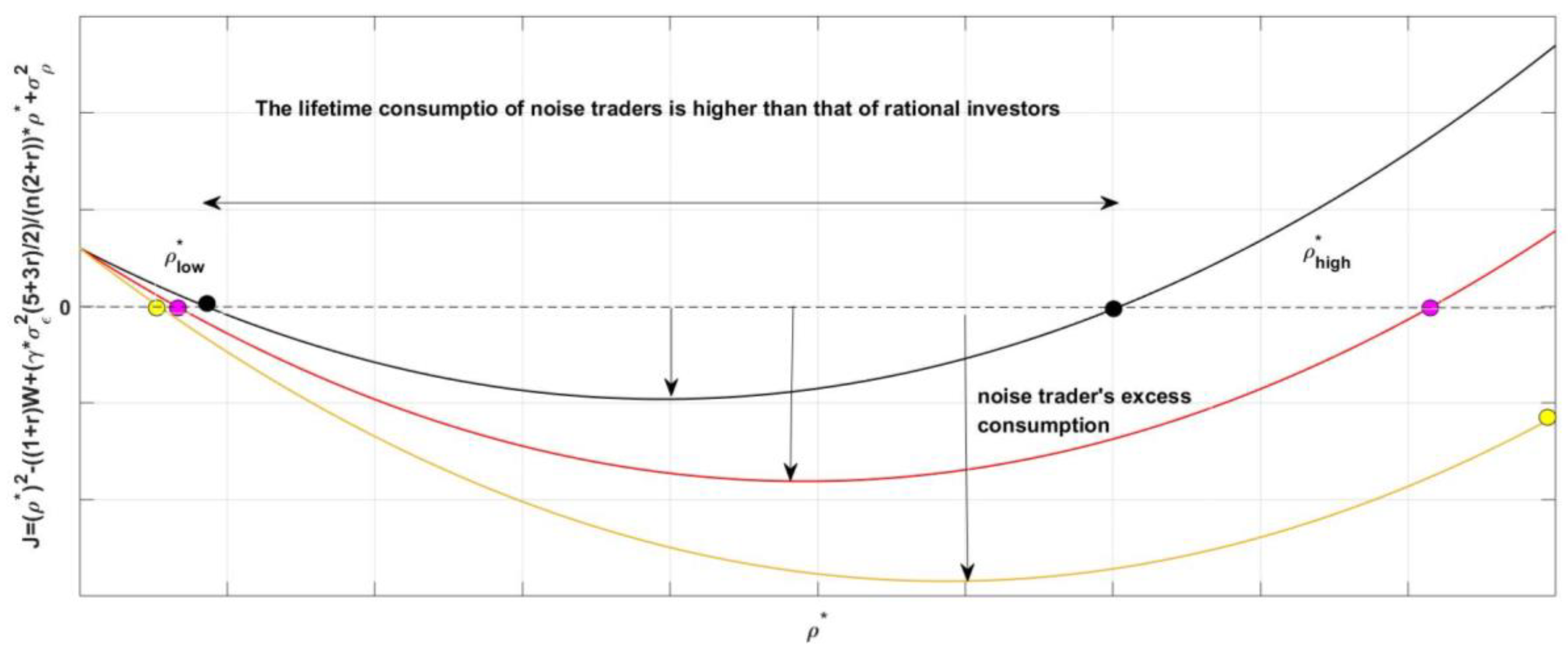
Therefore, the lifetime consumption of noise traders is higher than that of rational investors if ${\rho }_{low}^{*}\le {\rho }^{*}\le {\rho }_{high}^{*}$. We describe the scene more intuitively in the form of numerical simulation.

According to Figure 1, J is a parabola with upward opening, and it intersects with the abscissa to form a critical point where noise traders’ consumption is higher than that of rational investors. The intersection on the left is the lower limit of misconception, and the intersection on the right is the upper limit. False belief in $[{\rho }_{low}^{*},{\rho }_{high}^{*}]$ makes noise traders have higher welfare than rational investors. On the contrary, if ${\rho }^{*}>{\rho }_{high}^{*}$ or ${\rho }^{*}<{\rho }_{low}^{*}$, the welfare level of rational investors will exceed that of noise traders.

Next, we will examine the relationship between a series of parameter changes and the relative welfare of investors.

(1)

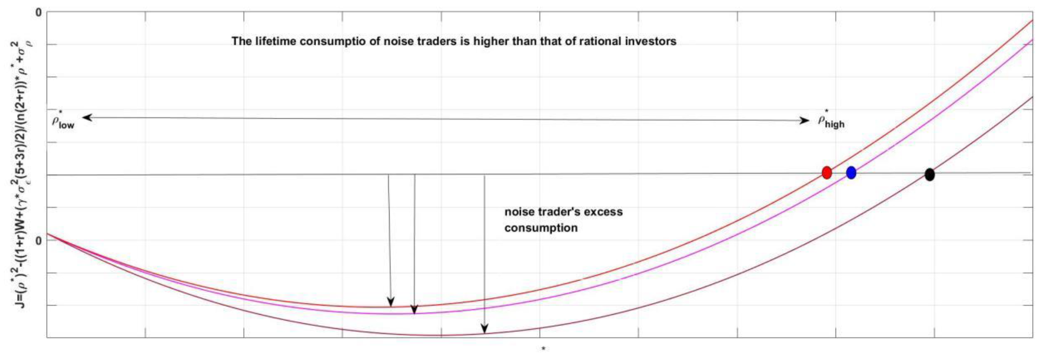
Effects of changes in fundamental risk

Since ${\sigma }_{\epsilon }^2={(\frac{n}{3 + 2r})}^2{\sigma }_{\rho }^2+{\sigma }_{\theta }^2$, with the increase in fundamental risk (${\sigma }_{\theta }^2$):

$$\frac{\partial {\rho }_{low}^{*}}{\partial {\sigma }_{\theta }^2}=\frac{5+3r}{4n(2+r)}\gamma \left\{1-\frac{\raisebox{1ex}{$(1 + r)W + (\frac{5 + 3r}{2})\gamma [{(\frac{n}{3 + 2r})}^2{\sigma }_{\rho }^2 + {\sigma }_{\theta }^2]$}\!\left/ \!\raisebox{-1ex}{$n(2 + r)$}\right.}{\sqrt{{(\raisebox{1ex}{$(1 + r)W + (\frac{5 + 3r}{2})\gamma [{(\frac{n}{3 + 2r})}^2{\sigma }_{\rho }^2 + {\sigma }_{\theta }^2]$}\!\left/ \!\raisebox{-1ex}{$n(2 + r)$}\right.)}^2-4{\sigma }_{\rho }^2}}\right\}$$

(47)

$$\frac{\partial {\rho }_{high}^{*}}{\partial {\sigma }_{\theta }^2}=\frac{5+3r}{4n(2+r)}\gamma \left\{1+\frac{\raisebox{1ex}{$(1 + r)W + (\frac{5 + 3r}{2})\gamma [{(\frac{n}{3 + 2r})}^2{\sigma }_{\rho }^2 + {\sigma }_{\theta }^2]$}\!\left/ \!\raisebox{-1ex}{$n(2 + r)$}\right.}{\sqrt{{(\raisebox{1ex}{$(1 + r)W + (\frac{5 + 3r}{2})\gamma [{(\frac{n}{3 + 2r})}^2{\sigma }_{\rho }^2 + {\sigma }_{\theta }^2]$}\!\left/ \!\raisebox{-1ex}{$n(2 + r)$}\right.)}^2-4{\sigma }_{\rho }^2}}\right\}$$

(48)

Therefore, the lower limit of noise traders’ false beliefs will decrease, and the upper limit will increase, which means that noise traders can obtain higher welfare. The result can be shown from Figure 2.

(2)

Effects of changes in risk-averse level

With the increase of risk averse level: $\frac{\partial {\rho }_{low}^{*}}{\partial \gamma }<0$,$\frac{\partial {\rho }_{high}^{*}}{\partial \gamma }>0$.

According to Figure 3, with the strengthening of investors’ risk aversion level, noise traders can obtain higher consumption than rational investors, which is consistent with the conclusion of DSSW [11]. The key here is that these two different types of agents share the same risk-aversion coefficient. Why does the strengthening of risk aversion make noise traders obtain higher consumption and rational investors’ consumption restrained? The reason is that rational investors, as reverse arbitrageurs, are committed to correcting the asset mispricing caused by noise traders. However, the strength and willingness to engage in reverse arbitrage will be pulled by risk aversion, which restricts its arbitrage power due to “fear” of losses. Noise traders are bound to be able to fully buy risky assets in the absence of arbitrage, obtain high returns by taking on high risks and finally make high consumption possible. In addition, although risk aversion will also affect the demand of noise traders, noise traders’ preference for risk assets is mainly related to their misconceptions, and the impact of risk aversion is extremely limited. Finally, noise traders can only seek high welfare.

(3)

Wealth endowment and relative consumption

As wealth levels rise: $\frac{\partial {\rho }_{low}^{*}}{\partial W}<0$,$\frac{\partial {\rho }_{high}^{*}}{\partial W}>0$, the result is exhibited in Figure 4.

Proposition 7.

The demand formulas for risk-free assets by noise traders and by rational investors are:

$${\lambda }_t^{f,n}=-\frac{(1-n){\rho }_t(W+\frac{\gamma }{2}{\sigma }_{\epsilon }^2+{\epsilon }_{t+1})}{\gamma {\sigma }_{\epsilon }^2(2+r)}$$

(49)

$${\lambda }_t^{f,i}=\frac{n{\rho }_t(W+\frac{\gamma }{2}{\sigma }_{\epsilon }^2+{\epsilon }_{t+1})}{\gamma {\sigma }_{\epsilon }^2(2+r)}$$

(50)

Although wealth endowment has nothing to do with the demand for risky assets, it can significantly affect the demand for risk-free assets. With the increase of wealth, $\frac{\partial {\lambda }_t^{i,n}}{\partial W}>0$, $\frac{\partial {\lambda }_t^{f,n}}{\partial W}<0$. Obviously, at this time, rational investors will increase the demand for risk-free assets and reduce the purchase of risky assets, while noise traders’ behavior is completely opposite. As rational investors hold more risk-free assets, noise traders will inevitably obtain higher returns due to holding more risky assets, so the increase in wealth endowment will also lead to higher welfare levels for noise traders.

(4)

Effect of noise traders’ market proportion

According to Figure 5, as the proportion of noise traders in the market increases: $\frac{\partial {\rho }_{low}^{*}}{\partial n}>0$,$\frac{\partial {\rho }_{high}^{*}}{\partial n}<0$.

Since the market share of noise traders increases, the scale and strength of rational investors will inevitably weaken. Why does this lead to the decline of noise traders’ consumption? When the market is dominated by noise traders, it is bound to be accompanied by high noise trader risk. At this time, there is no so-called risk-free arbitrage opportunity for the two types of agents: Although they believe that there exists mispricing of risk assets at this time, no one is willing to establish arbitrage positions due to the future uncertainty caused by noise trader risk. Therefore, noise traders will buy a large number of risky assets based on false beliefs, and the asset price will rise with the increase in the proportion of noise traders (available from formula (26)), but this will lead to reduced returns. As a result, the increase in the proportion of noise traders has led to a lower consumption of noise traders. In the face of the risk of noise traders, rational investors choose to use their wealth for savings rather than investment, which has improved their consumption.

3. Comparison with Similar Studies

Since Keynes [48], there has been a large number of studies on the impacts of expected changes on consumption; especially since the Great Depression, expected change has become one of the factors leading to sharp drops in asset prices [49]. Recently, the economic sentiment caused by the COVID-19 pandemic may have affected consumption even after the elimination of the virus because there are scars on people’s belief in rare disasters [50].

Unlike the existing literature, we study the situation of optimistic belief rather than pessimistic belief, and the explanatory factor we use is noise trader risk, which can also be called investor sentiment rather than economic sentiment. Additionally, the existing literature is mainly empirical, lacking theoretical models. The weakness of this article lies in the lack of support from empirical data; this is because we cannot find suitable sample data in China, especially high-frequency data. However, the conclusion we obtain is similar to that of Zhang Dixin et al. [47], who proved that most noise traders have a gambler mentality. When there is a positive return on the stock market, they do not convert the return into real consumption but reduce consumption and increase investment in the stock market in order to obtain more stock market returns.

4. Conclusions

This paper extends the model of DSSW [11] and discusses the impact of noise trader risk on total consumption and consumption levels of different types of investors. Although the model constructed still includes rational investors and noise traders, the foothold is expanded from asset price to consumption, trying to discuss the impacts of financial market fluctuations on the real economy from the perspective of behavior. The main conclusions are as follows:

(1)

The individual consumption of investors follows a random walk process with drift term, but the total market consumption is stable;

(2)

If noise traders have optimistic beliefs about asset prices, when the noise trading intensity is higher than a certain level, noise trader risk will have a restraining effect on the total consumption;

(3)

For current consumption, if the noise traders show optimistic deviation for asset value, the consumption in period t will be higher than the market average consumption, and the consumption of rational investors in period t will be lower than the market average consumption. In other words, noise traders will increase consumption in period t and reduce consumption in period t + 1, while rational investors will reduce consumption in period t and increase consumption in period t + 1;

(4)

For current consumption, if noise traders do not show belief bias, the consumption of rational investors will always be higher than the average level of noise traders and the market;

(5)

If the false belief of noise traders is between, the lifetime consumption of noise traders will be higher than that of rational investors and the average market consumption. With increases in fundamental risk, risk aversion and wealth endowment, the range will become larger, and noise traders will get higher excess consumption, whereas as the proportion of noise traders increases, the excess consumption of noise traders will decrease accordingly.

(6)

Most of the existing behavioral finance research examines asset price volatility from the perspective of investor sentiment or sentiment feedback. Few scholars discuss the real economy from an irrational perspective, especially the changes in consumption that can reflect the level of social welfare. This paper helps to expand behavioral finance research and clarify the relationships between financial markets and the real economy, and it has rich theoretical and practical significance.

There are no completely rational investors and irrational investors. It may be more practical to build an investment agent that includes “rational economic man” and “animal spirit” at the same time. If we can refer to the ideas of Barberis et al. (2018), it will further increase the theoretical value of the article and help reveal more laws and puzzles about the market. In addition, if we can increase empirical research on theoretical analysis, it will further confirm the rationality and robustness of the conclusions. Finally, the manifestations of noise traders are not limited to DSSW (1990a). If we can measure them through overconfidence and extrapolation expectations, this may be a more interesting focus.

References

1. Hansman, C.; Hong, H.; Jiang, W.; Liu, Y.J.; Meng, J.J. Riding the Credit Boom 2018 (No. W24586); National Bureau of Economic Research: Cambridge, MA, USA, 2018. [Google Scholar]
2. Zhang, Y.X.; Jia, Q.M.; Chen, C. Risk attitude, financial literacy and household consumption: Evidence from stock market crash in China. Econ. Model. 2021, 94, 995–1006. [Google Scholar] [CrossRef]
3. Hu, C.S.; Peng, Z.; Chi, Y.C. Feedback trading, Trading inducement and Asset price behavior. Econ. Res. J. 2017, 52, 189–202. [Google Scholar]
4. Fama, E. Efficient Capital Markets: A Review of Theory and Empirical Work. J. Financ. 1970, 25, 383–417. [Google Scholar] [CrossRef]
5. Barberis, N.C. Psychology-Based Models of Asset Prices and Trading Volume. In Handbook of Behavioral Economics: Applications and Foundations 1; North-Holland: Amsterdam, The Netherlands, 2018; Volume 1, pp. 79–175. [Google Scholar]
6. Black, F. Noise. J. Financ. 1986, 41, 529–543. [Google Scholar] [CrossRef]
7. Shleifer, A.; Vishny, R. The limits to arbitrage. J. Financ. 1997, 52, 35–55. [Google Scholar] [CrossRef]
8. Pontiff, J. Costly arbitrage and the myth of idiosyncratic risk. J. Account. Econ. 2006, 42, 35–52. [Google Scholar] [CrossRef]
9. Barroso, P.; Detzel, A. Do limits to arbitrage explain the benefits of volatility-managed portfolios? J. Financ. Econ. 2021, 140, 744–767. [Google Scholar] [CrossRef]
10. Priem, R. An Exploratory Study on the Impact of the COVID-19 Confinement on the Financial Behavior of Individual Investors. Econ. Manag. Financ. Mark. 2021, 16, 9–40. [Google Scholar]
11. De Long, J.; Shleifer, A.S.; Waldman, R. Noise trader risk in financial markets. J. Political Econ. 1990, 98, 703–738. [Google Scholar] [CrossRef]
12. Ding, W.; Mazouz, K.; Wang, Q. Investor sentiment and the cross-section of stock returns: New theory and evidence. Rev. Quant. Financ. Account. 2019, 53, 493–525. [Google Scholar] [CrossRef] [Green Version]
13. Morales, L.; Gray, G.; Rajmil, D. Emerging Risks in the FinTech Industry—Insights from Data Science and Financial Econometrics Analysis. Econ. Manag. Financ. Mark. 2022, 17, 9–36. [Google Scholar]
14. Glaeser, E.L.; Nathanson, C.G. An extrapolative model of house price dynamics. J. Financ. Econ. 2017, 126, 147–170. [Google Scholar] [CrossRef] [Green Version]
15. Barberis, N.C.; Greenwood, R.; Jin, L.; Shleifer, A. Extrapolation and Bubbles. J. Financ. Econ. 2018, 129, 203–227. [Google Scholar] [CrossRef]
16. Chinco, A. The Ex-Ante Likelihood of Bubbles; Working Paper; University of Chicago: Chicago, IL, USA, 2020. [Google Scholar]
17. DeFusco, A.A.; Nathanson, C.G.; Zwick, E. Speculative Dynamics of Prices and Volume; Working Paper; Northwestern University: Evanston, IL, USA, 2020. [Google Scholar]
18. Liao, J.C.; Peng, C.; Zhu, N. Extrapolative Bubbles and Trading Volume. Rev. Financ. Stud. 2022, 35, 1682–1722. [Google Scholar] [CrossRef]
19. De Long, J.B.; Shleifer, A.; Summers, L.; Waldmann, R. Positive Feedback Investment Strategies and Destabilizing Rational Speculation. J. Financ. 1990, 45, 375–395. [Google Scholar] [CrossRef] [Green Version]
20. Baker, M.; Wurgler, J. Investor sentiment and the cross-section of stock returns. J. Financ. 2006, 61, 1645–1680. [Google Scholar] [CrossRef] [Green Version]
21. Baker, M.; Wurgler, J. Investor sentiment in the stock market. J. Econ. Perspect. 2007, 21, 129–151. [Google Scholar] [CrossRef] [Green Version]
22. Brown, G.W.; Cliff, M.T. Investor sentiment and asset valuation. J. Bus. 2005, 78, 405–440. [Google Scholar] [CrossRef]
23. Fisher, K.L.; Statman, M. Investor sentiment and stock returns. Financ. Anal. J. 2000, 56, 16–23. [Google Scholar] [CrossRef]
24. Da, Z.; Engelberg, J.; Gao, P. In search of attention. J. Financ. 2011, 66, 1461–1499. [Google Scholar] [CrossRef]
25. Bathia, D.; Bredin, D. An examination of investor sentiment effect on G7 stock market returns. Eur. J. Financ. 2013, 19, 909–937. [Google Scholar] [CrossRef]
26. Wang, W.Z.; Su, C.; Duxdbury, D. Investor sentiment and stock returns: Global evidence. J. Empir. Financ. 2021, 63, 365–391. [Google Scholar] [CrossRef]
27. Berger, D.; Turtle, H.J. Sentiment Bubbles. J. Financ. Mark. 2015, 23, 59–74. [Google Scholar] [CrossRef]
28. Steindel, C.; Ludvigson, S.C. How important is the stock market effect on consumption? Econ. Policy Rev. 1999, 5, 29–51. [Google Scholar]
29. Poterba, J.M. Stock market wealth and consumption. J. Econ. Perspect. 2000, 14, 99–118. [Google Scholar] [CrossRef]
30. Mehra, Y.P. The wealth effect in empirical life-cycle aggregate consumption equations. FRB Richmond Econ. Q. 2001, 87, 45–68. [Google Scholar]
31. Dvornak, N.; Kohler, M. Housing wealth, stock market wealth and consumption: A panel analysis for Australia. Econ. Rec. Econ. Soc. Aust. 2007, 83, 117–130. [Google Scholar] [CrossRef]
32. Funke, N. Is there a stock market wealth effect in emerging markets? Econ. Lett. 2004, 83, 417–421. [Google Scholar] [CrossRef]
33. Fisher, L.A.; Voss, G.M. Consumption, wealth and expected stock returns in Australia. Econ. Rec. Econ. Soc. Aust. 2004, 80, 359–372. [Google Scholar] [CrossRef]
34. Lettau, M.; Ludvigson, S.C. Understanding trend and cycle in asset values: Reevaluating the wealth effect on consumption. Am. Econ. Rev. 2004, 94, 276–299. [Google Scholar] [CrossRef] [Green Version]
35. Labhard, V.; Sterne, G.; Young, C. Wealth and Consumption: An Assessment of the International Evidence; Bank of England Working Paper. No. 275; Bank of England: London, UK, 2005. [Google Scholar]
36. Paiella, M. The stock market, housing and consumer spending: A survey of the evidence on wealth effects. J. Econ. Surv. 2009, 23, 947–973. [Google Scholar] [CrossRef]
37. Singh, B. How important is the stock market wealth effect on consumption in India? Empir. Econ. 2012, 42, 915–927. [Google Scholar] [CrossRef]
38. Hudomiet, P.; Kezdi, G.; Willis, R.J. Stock market crash and expectations of American households. J. Appl. Econ. 2011, 26, 393–415. [Google Scholar] [CrossRef] [PubMed] [Green Version]
39. Hoffmann, A.O.; Post, T.; Pennings, J.M. Individual investor perceptions and behavior during the financial crisis. J. Bank. Financ. 2013, 37, 60–74. [Google Scholar] [CrossRef]
40. Jensen, T.L.; Johannesen, N. The consumption effects of the 2007–2008 financial crisis: Evidence from households in Denmark. Am. Econ. Rev. 2017, 107, 3386–3414. [Google Scholar] [CrossRef]
41. Tsai, I.C. Wealth effect and investor sentiment. North Am. J. Econ. Financ. 2016, 38, 111–123. [Google Scholar] [CrossRef]
42. Kliestik, T.; Valaskova, K.; Lăzăroiu, G.; Kovacova, M.; Vrbka, J. Remaining Financially Healthy and Competitive: The Role of Financial Predictors. J. Compet. 2020, 12, 74–92. [Google Scholar] [CrossRef]
43. Yin, Z.; Zhang, H. Financial literacy and households wealth inequality in China: Evidence from CHFS data. Stud. Int. Financ. 2017, 10, 76–86. [Google Scholar]
44. Chen, G.; Kim, K.A.; Nofsinger, J.R.; Rui, O.M. Trading performance, disposition effect, overconfidence, representativeness bias, and experience of emerging market investors. J. Behav. Decis. Mak. 2007, 20, 425–451. [Google Scholar] [CrossRef]
45. Narayan, P.K.; Narayan, S.; Westerlund, J. Do order imbalances predict Chinese stock returns? New evidence from intraday data. Pac. Basin Financ. J. 2015, 34, 136–151. [Google Scholar] [CrossRef]
46. Narayan, P.K.; Ranjeeni, K.; Bannigidadmath, D. New evidence of psychological barrier from the oil market. J. Behav. Financ. 2017, 18, 457–469. [Google Scholar] [CrossRef]
47. Zhang, D.X.; Liu, Z.X.; Xu, Z.Y. A Study of the impact of Stock Market Returns, Volatility and Liquidity on Urban Residents’ Consumption. Contemp. Financ. Econ. 2016, 7, 46–57. [Google Scholar]
48. Keynes, J. The General Theory of Employment, Interest and Money; Macmillan Cambridge University Press: Cambridge, UK, 1936. [Google Scholar]
49. Adam, K.; Marcet, A.; Beutel, J. Stock price booms and expected capital gains. Am. Econ. Rev. 2017, 107, 2352–2408. [Google Scholar] [CrossRef]
50. Kozlowski, J.; Veldkamp, L.; Venkateswaran, V. Scarring Body and Mind: The Long-Term Belief-Scarring Effects of COVID-19; FRB St. Louis Working Paper; National Bureau of Economic Research: Cambridge, MA, USA, 2020. [Google Scholar]
Figure 1. This figure shows the upper and lower limits of average false belief of noise traders. For the parameters involved, we refer to Barberis et al. [15] for the following assignment: r = 0.25 , W = 5 , n = 0.4 , γ = 0.1 , σ ε 2 = 3 , σ ρ 2 = 6 .
Mathematics 10 03873 g001
Figure 2. The effect of fundamental risk volatility.
Mathematics 10 03873 g002
Figure 3. The effect of risk averse changes.
Mathematics 10 03873 g003
Figure 4. The effects of changes in wealth endowment.
Mathematics 10 03873 g004
Figure 5. The effect of the change in the proportion of noise traders.
Mathematics 10 03873 g005
Publisher’s Note: MDPI stays neutral with regard to jurisdictional claims in published maps and institutional affiliations.