Bayesian and Frequentist Approaches for a Tractable Parametric General Class of Hazard-Based Regression Models: An Application to Oncology Data

Abstract

In this study, we consider a general, flexible, parametric hazard-based regression model for censored lifetime data with covariates and term it the “general hazard (GH)” regression model. Some well-known models, such as the accelerated failure time (AFT), and the proportional hazard (PH) models, as well as the accelerated hazard (AH) model accounting for crossed survival curves, are sub-classes of this general hazard model. In the proposed class of hazard-based regression models, a covariate’s effect is identified as having two distinct components, namely a relative hazard ratio and a time-scale change on hazard progression. The new approach is more adaptive to modelling lifetime data and could give more accurate survival forecasts. The nested structure that includes the AFT, AH, and PH models in the general hazard model may offer a numerical tool for identifying which of them is most appropriate for a certain dataset. In this study, we propose a method for applying these various parametric hazard-based regression models that is based on a tractable parametric distribution for the baseline hazard, known as the generalized log-logistic (GLL) distribution. This distribution is closed under all the PH, AH, and AFT frameworks and can incorporate all of the basic hazard rate shapes of interest in practice, such as decreasing, constant, increasing, V-shaped, unimodal, and J-shaped hazard rates. The Bayesian and frequentist approaches were used to estimate the model parameters. Comprehensive simulation studies were used to evaluate the performance of the proposed model’s estimators and its nested structure. A right-censored cancer dataset is used to illustrate the application of the proposed approach. The proposed model performs well on both real and simulation datasets, demonstrating the importance of developing a flexible parametric general class of hazard-based regression models with both time-independent and time-dependent covariates for evaluating the hazard function and hazard ratio over time.

1. Introduction

One of the main goals of censored time-to-event data analysis with covariates is to find and quantify the relationship between the baseline hazard rate function (hrf) and the covariates so that the covariates can be employed in disease prevention and management [1,2,3,4,5]. The assumption leads to hazard-based regression models, and the study goal is to estimate a vector of regression coefficients for the components of covariates.

Cox [6] developed a hazard-based regression model in which the covariate has a multiplicative relationship with the hrf, and is called the proportional hazard $\left(\mathrm{PH}\right)$ model. The $\mathrm{PH}$ model is without a doubt the most widely used in practice. Let $h(t;x)$ be the hrf for a subject with $x={\left(x_1,x_2,\dots ,x_p\right)}^T$ variables, and $h_0\left(t\right)$ be the baseline hrf for those with $x=0$. The following is a formula for the Cox PH model:

$$h(t;x)=h_0\left(t\right)·\psi (\beta ·x)=h_0\left(t\right)e^{x^{\prime }\beta },$$

(1)

where $\psi$ is a positive link function with $\psi \left(0\right)=1$, most often the exponential function is used to represent the link function of the covariates; $\beta ={\left({\beta }_1,{\beta }_2,\dots ,{\beta }_p\right)}^T$ is the vector of the regression coefficients, $e^{{\beta }_j}$ denotes the hazard ratio resulting from an increase in the jth covariate by one unit. The Cox PH model leads to the estimation of $\beta$ by means of a “partial likelihood” approach [7].

The Cox PH model is usually used to model censored lifetime data. However, there may be some benefits to using parametric $\mathrm{PH}$ models for such data. According to Hjort [8], the success of the Cox PH regression model may have had the unintended consequence of practitioners paying too little attention to the baseline hazard. If proved to be acceptable, a parametric version of the Cox model would allow for more exact estimation of survival probability, while also contributing to a better understanding of the phenomenon under investigation. Parametric $\mathrm{PH}$ models, for example, which might be a challenge with the Cox PH model, can sometimes be handled simply, and visualizations of the hrf are considerably easier. To accommodate variable hrf forms, modifications to the log-logistic and Weibull models are presented. For example, exponentiated-Weibull [9], sine Kumaraswamy–Weibull [10], arctan–Weibull [11], exponentiated generalized cosine–Weibull [12], secant Kumaraswamy–Weibull [13], tan log-logistic [14], and the generalized log-logistic [15] models.

When the Cox PH model proportionality assumption is not satisfied, flexible parametric non-proportional hazards can be relaxed. For example, the accelerated failure time (AFT) model can be considered [16]. The AFT model can be written as:

$$h(t;x)=h_0\left(t{e}^{x^{\prime }\beta }\right)e^{x^{\prime }\beta }.$$

(2)

The AFT assumption in Equation (2) postulates that the covariates have time-dependent and non-proportional effects on the hazard rate, while PH assumption in Equation (1) postulates that the covariates have time-independent and proportional effects.

The PH and AFT models have been widely employed in a variety of time-to-event analysis applications. These models, despite their popularity, are unsuitable for handling time-to-event data with crossed survival and hazard curves [17]. Chen and Weng [18] presented a new class of hazard-based regression models, known as the accelerated hazard (AH) model, that may be used to analyze crossing survival curves. The AH model can be written as:

$$h(t;x)=h_0\left(t{e}^{x^{\prime }\beta }\right).$$

(3)

To describe the shift in hazard progression across time, the AH assumption in Equation (3) assumes that the covariates have a time-scale change to the hazard rate function. The $\mathrm{AH}$ model has the advantage of being non-proportional, it can accept the phenomenon of identical hazards at time $t=0$, which is common in randomized clinical trials.

As a result, the relationship between covariates and baseline hazard can be described as follows: covariates with a “proportional” effect on the hrf must be time-independent and capable of scaling up the baseline hrf, whereas covariates with a “non-proportional” effect on the hrf must be time-dependent or interact with time in the baseline hrf. As a result, whereas the influence of a time-independent covariate on the hrf varies over time, the effect of a time-independent covariate on the hrf remains constant.

Hence, when creating the link between the covariates and the hrf, we have four options: time-dependent, time-independent, proportional, or non-proportional. As a result, neither the AFT, AH, or PH models can enable some factors to have proportional and time-dependent impacts on the hazard while others have non-proportional and time-dependent effects in one model [19]. To solve this issue, the goal of this work is to introduce a tractable parametric general class of hazard-based regression models for overall survival data that includes the AFT, AH, and PH as special cases, which will subsequently be used to model right-censored cancer datasets with or without crossover survival curves.

The motivating ideas behind our work on Bayesian and frequentist approaches for the general class of hazard-based regression models with GLL baseline distribution are as follows: (i) the baseline continuous probability distributions closed under the PH and AFT frameworks have drawbacks in that most of them are not adaptable enough to take into account both monotone and non-monotone hazard rates; (ii) for statistical inference, the Bayesian approach does not depend on asymptotic approximations; to the author’s knowledge, there are no previous studies for the Bayesian inference of the general class of parametric hazard-based regression models; (iii) due to the accessibility of software, Bayesian application for hazard-based complex models is considerably easier and simpler than the frequentist approach; (iv) if the baseline hazard distribution is valid and correct, parametric hazard-based regression models may yield more accurate estimates than semi-parametric hazard-based regression models; and, last but just not least, (v) what sets our work apart and appeals to healthcare professionals, epidemiologists, bio-statisticians, and other applied researchers in numerous fields is the use of modified distributions that may accommodate different hazard rate shapes data.

Based on the above-mentioned motivations and discussions, the main purpose of this paper is to introduce a general parametric hazard-based regression model with a generalized log-logistic baseline distribution. So, presenting the parametric GH class of hazard-based regression models and their special cases using GLL baseline hazard, deriving the probabilistic functions for the GH model, formulating and interpreting all the special cases, applying the Bayesian and frequentist inference procedures, developing computational algorithms to fit the proposed GH model, estimating the covariate effect on the hazard rate, and applying it to a right-censored cancer dataset is the novelty of the study.

The rest of this text is folded as follows: Section 2 describes the proposed GH model formulation, assumptions, its nested structure, and its probabilistic functions. Section 3 lists the special cases of the general hazard model and their probabilistic functions. The parameter interpretations of the sub-models are discussed in Section 4. Section 5 reviews the generalized log-logistic (GLL) distribution and its special cases. Section 6 presents the inferential approaches of the proposed GH model. Two extensive simulation studies are presented in Section 7. Section 8 displays two right-censored cancer datasets, one of which contains crossover survival curves. The final Section 9 contains the major conclusion, final remarks, and discussion of future work.

2. Model Formulation

2.1. Review of Current Literature and Recent Research

Prior to the model formulation, we discuss the state of scientific progress in the context of current survival models. Specifically, we look at the work that has been completed in relation to the closely related extended hazard (EH) and generalized hazard (GH) models. The EH model is actually very similar to the GH model; the only distinction is that the EH model was developed before the development of the AH model. In the study of censored lifetime data with covariates, Ciampi and Etazadi-Amoli [20] constructed a universal model for evaluating the PH and the AFT hypothesis. Then, using spline approximation, Etazadi-Amoli and Ciampi [21] proposed an EH model for censored lifetime data with variables.

Following the research completed by Etazadi-Amoli and Ciampi, Louzada-Neto [22] proposed an EH regression model that permits the spread parameter to rely on covariates. For EH models, Louzada-Neto [23] presented a simple Bayesian analysis. Then, after the development of the AH model, Chen and Jewell [24] developed the GH model, which combines the EH model with the AH model, another hazard-based model. An extended linear EH model with applicability to time-dependent covariates was proposed by [25]. Tong et al. [26] addressed a few inferential research questions in the semi-parametric GH model. The modification of the GH model was discussed by Wang et al. [19] in the context of time-independent and time-dependent factors.

The majority of the work created in relation to GH models dealt with semi-parametric models. The parametric GH regression models for the relative survival data were recently examined by [3]. Other efforts for the GH models were discussed by Li et al. [27] by extending the GH model to a spatial model. Finally, a mixed-effect GH model was created by Rubio and Drikvandi [28] to include clustered survival data.

There is a research gap following the current literature that needs to be filled. Both the application of the GH model to the overall survival data and the field of statistical inference for the Bayesian approach are unresolved issues that need to be resolved. Here, we suggest a parametric GH model to close that gap, and we estimate the model’s parameters using both maximum likelihood estimation (MLE) and Bayesian methods.

2.2. Model Formulation

The hrf and the cumulative hazard function (chf), rather than the probability density function (pdf) and the cumulative distribution function (cdf) are typically used to interpret the most common parametric hazard-based regression models.

Assume that x is a vector of covariates, T is a non-negative random variable that represents the amount of time till the occurrence of an event of concern, and $\psi \left(x\right)$ is the link function for the covariates, which is most often employed as an exponential or (log-linear function) $e^{x^{{}^{\prime }}\beta }$, where $\beta$ is a vector of regression coefficients. Ciampi and Etazadi-Amoli [20] developed a generalized version of the PH and AFT models to incorporate more versatile interaction terms in relation to the covariates and time.

The hrf and chf of the general class of hazard-based regression models are expressed as follows:

$$h_{GH}(t;x)=h_0\left(t\psi \left({\mathit{x}}^{\prime }{\mathsf{\beta }}_{\mathbf{1}}\right)\right)\psi \left({\mathit{x}}^{\prime }{\mathsf{\beta }}_2\right)=h_0\left(t{e}^{x^{\prime }{\beta }_1}\right)e^{x^{\prime }{\beta }_2},$$

(4)

$$H_{GH}(t;x)=H_0\left(t\psi \left({\mathit{x}}^{\prime }{\mathsf{\beta }}_{\mathbf{1}}\right)\right)\psi \left(-{\mathit{x}}^{\prime }{\mathsf{\beta }}_{\mathbf{1}}+{\mathit{x}}^{\prime }{\mathsf{\beta }}_2\right)=H_0\left(t{e}^{x^{\prime }{\beta }_1}\right)e^{x^{\prime }{\beta }_2-x^{\prime }{\beta }_1},$$

(5)

where $h_0\left(t\right)$ and $H_0\left(t\right)$ are called the baseline hazard and the baseline cumulative hazard rate functions, respectively; $h_{GH}(t;x)$ is the hrf at time t, and $H_{GH}(t;x)$ is the cumulative hrf at time t.

2.3. Nested Structure of the GH Model

The importance of the general class of parametric hazard-based regression model is that it represents a $\mathrm{GH}$ structure that contains, as special cases, the proportional hazard $\left(\mathrm{PH}\right)$, accelerated hazard $\left(\mathrm{AH}\right)$, and the accelerated failure time ($\mathrm{AFT})$ models. To be more clear, the following relations hold:

i.

If ${\beta }_1=0$, then $\mathrm{GH}=\mathrm{PH}$;

ii.

If ${\beta }_2=0$, then $\mathrm{GH}=\mathrm{AH}$;

iii.

If ${\beta }_1={\beta }_2$, then $\mathrm{GH}=\mathrm{AFT}$.

Hence, the $\mathrm{GH}$ model can be used as a numerical tool to determine which of them is more appropriate for a given censored survival data. The nested structure of the model illustrates the richness of the GH class and motivates its investigation [21].

2.4. Model Assumption

The basic assumption of the general class of parametric hazard-based regression models is that the effect of covariates on the hrf is identified as having two separate components, namely:

i.

A time-scale change in the hrf;

ii.

A relative hazards ratio.

$$h_{GH}(t;x)=h_0\left(t{e}^{x^{\prime }{\beta }_1}\right)e^{x^{\prime }{\beta }_2}.$$

i.

Time-dependent and time-independent (time-fixed) covariates;

ii.

Proportional and non-proportional hazards separately.

for evaluating the hrf and hazard ratio over time [24].

The assumption of the special cases is different in nature. For instance, the PH framework postulates that the covariates multiply the hrf, causing the hrf to fluctuate in level [29,30]. The $\mathrm{AH}$ framework postulates that each covariate has a time-dependent effect since it states that the effect of a unit change in a covariate affects the time scale of the baseline hrf [18]. In the AFT framework, it is postulated that the covariates have an effect both on the hazard and the time scale [31]. Note that, the AH, AFT, and PH models coincide for the case when the baseline hazard is the Weibull distribution [3].

2.5. Probabilistic Functions for the GH Model

In this section, we derive the most common probabilistic functions for the GH model. The other probabilistic functions for the model with Equations (4) and (5) are computed as follows:

The survival function (sf) of the GH model is computed as follows:

$$S_{GH}(t;x)=S_0{\left(t{e}^{x^{\prime }{\beta }_1}\right)}^{e^{x^{\prime }{\beta }_2-x^{\prime }{\beta }_1}}.$$

(6)

where $S_0(.)$ is the baseline survival function.

The cdf of the $\mathrm{GH}$ model is expressed as follows:

$$F_{GH}(t;x)=1-S_{GH}(t;x)=1-S_0{\left(t{e}^{x^{\prime }{\beta }_1}\right)}^{e^{x^{\prime }{\beta }_2-x^{\prime }{\beta }_1}}.$$

(7)

The pdf of the GH model can be obtained by using:

$$f_{GH}(t;x)=h_0\left(t{e}^{x^{\prime }{\beta }_1}\right)e^{x^{\prime }{\beta }_2}{S}_0{\left(t{e}^{x^{\prime }{\beta }_1}\right)}^{e^{x^{\prime }{\beta }_2-x^{\prime }{\beta }_1}}.$$

(8)

3. Special Cases of the GH Model

In this section, the three common sub-models for the general class of the hazard-based regression models are discussed.

3.1. Proportional Hazard Model

In the GH model framework, if ${\beta }_1=0$, then $\mathrm{GH}=\mathrm{PH}$ framework. Hence, the hrf is expressed as follows:

$$h_{PH}(t;x)=h_0\left(t\right)e^{x^{\prime }\beta }.$$

(9)

The chf is expressed as:

$$H_{PH}(t;x)=H_0\left(t\right)e^{x^{\prime }\beta }.$$

(10)

The sf of the PH model is computes as follows:

$$S_{PH}(t;x)=S_0{\left(t\right)}^{e^{x^{\prime }\beta }}.$$

(11)

The cdf of the PH model is expressed as follows:

$$F_{PH}(t;x)=1-S_{PH}(t;x)=1-S_0{\left(t\right)}^{e^{x^{\prime }\beta }}.$$

(12)

The pdf of the $\mathrm{PH}$ model can be obtained by using:

$$f_{PH}(t;x)=f_0\left(t\right)e^{x^{\prime }\beta }{S}_0{\left(t\right)}^{e^{x^{\prime }\beta -1}}$$

(13)

3.2. Accelerated Hazard Model

In the $\mathrm{GH}$ model framework, if ${\beta }_2=0$, then $\mathrm{GH}=\mathrm{AH}$ framework. Hence, the hrf is expressed as follows:

$$h_{AH}(t;x)=h_0\left(t{e}^{x^{\prime }\beta }\right).$$

(14)

The chf is expressed as:

$$H_{AH}(t;x)=H_0\left(t{e}^{x^{\prime }\beta }\right)e^{-x^{\prime }\beta }.$$

(15)

The sf of the AH model is computed as follows:

$$S_{AH}(t;x)=S_0{\left(t{e}^{x^{\prime }\beta }\right)}^{e^{-x^{\prime }\beta }}.$$

(16)

The cdf of the AH model is expressed as follows:

$$F_{AH}(t;x)=1-S_{AH}(t;x)=1-S_0{\left(t{e}^{x^{\prime }\beta }\right)}^{e^{-x^{\prime }\beta }}.$$

(17)

The pdf of the $\mathrm{AH}$ model can be obtained by using:

$$f_{AH}(t;x)=f_0\left(t{e}^{x^{\prime }\beta }\right)S_0{\left(t{e}^{x^{\prime }\beta }\right)}^{e^{-x^{\prime }\beta }}.$$

(18)

3.3. Accelerated Failure Time Model

In the GH model framework, if ${\beta }_1={\beta }_2$, then GH = AFT framework. Hence, the hrf is expressed as follows:

$$h_{AFT}(t;x)=h_0\left(t{e}^{x^{\prime }\beta }\right)e^{x^{\prime }\beta }.$$

(19)

The chf is expressed as:

$$H_{AFT}(t;x)=H_0\left(t{e}^{x^{\prime }\beta }\right).$$

(20)

The sf of the AFT model is computed as follows:

$$S_{AFT}(t;x)=S_0\left(t{e}^{x^{\prime }\beta }\right)$$

(21)

The cdf of the AFT model is expressed as follows:

$$F_{AFT}(t;x)=1-S_{AFT}(t;x)=1-S_0\left(t{e}^{x^{\prime }\beta }\right).$$

(22)

The pdf of the AFT model can be obtained by using:

$$f_{AFT}(t;x)=f_0\left(t{e}^{x^{\prime }\beta }\right)e^{x^{\prime }\beta }.$$

(23)

The $\mathrm{GH}$ model is a general class that includes the $\mathrm{PH},\mathrm{AFT}$, and $\mathrm{AH}$ models as special examples. More specifically, if ${\beta }_1=0$, then $\mathrm{GH}=\mathrm{PH}$; if ${\beta }_2=0$, then $\mathrm{GH}=\mathrm{AH}$; and if ${\beta }_2={\beta }_1$, then GH = AFT [3,20,21].

4. Parameter Interpretation for the Parametric Hazard-Based Regression Models

In this section, it is crucial to determine if a positive coefficient of a covariate can monotonically raise the time scale or lower the hazard in order to ensure that the broad class of hazard-based regression models has a plausible interpretation.

4.1. Proportional Hazard Model

In this sub-section, we start the interpretation of the parameters of the PH model, as this will facilitate the interpretation of the general class model. if ${\beta }_1=0$, then the GH model is the same as that in a PH model:

$$h(t;x)=h_0\left(t\right)e^{x^{\prime }\beta },$$

(24)

$$H(t;x)=H_0\left(t\right)e^{x^{\prime }\beta },$$

(25)

$$\frac{dH(t;x)}{dx}=\beta e^{x^{\prime }\beta }{H}_0\left(t\right),$$

(26)

where $H_0\left(t\right)$ is an increasing function that takes a value greater than 0. When $\beta >$ 0, $\frac{dH(t;x)}{dx}>0$, showing that when the covariate x increases, the hazard increases and the survival time decreases.

4.2. Accelerated Failure Time Model

In the GH model, if the covariate ${\beta }_2={\beta }_1$, the GH model is the same as the AFT model. Hence,

$$h(t;x)=h_0\left(t{e}^{x^{\prime }\beta }\right)e^{x^{\prime }\beta },$$

(27)

$$H(t;x)=H_0\left(t{e}^{x^{\prime }\beta }\right),$$

(28)

$$\frac{dH(t;x)}{dx}=\beta t{e}^{x^{\prime }\beta }{H}_0^{\prime }\left(t{e}^{x^{\prime }\beta }\right),$$

(29)

Since $H_0(.)$ is an increasing function, $H_0^{\prime }(.)$ Is greater than 0. When $\beta >0$, $\frac{dH(t;x)}{dx}>0$, showing that when the covariate x increases, the hazard increases and the survival time decreases.

4.3. Accelerated Hazard Model

In the $\mathrm{GH}$ model, if the covariate ${\beta }_2=0$, the GH model is the same as the $\mathrm{AH}$ model. Hence,

$$h(t;x)=h_0\left(t{e}^{x^{\prime }\beta }\right),$$

(30)

$$H(t;x)=e^{-x^{\prime }\beta }{H}_0\left(t{e}^{x^{\prime }\beta }\right),$$

(31)

$$\frac{dH(t;x)}{dx}=-\beta e^{-x^{\prime }\beta }\left[H_0\left(t{e}^{x^{\prime }\beta }\right)-t{e}^{x^{\prime }\beta }{H}_0^{\prime }\left(t{e}^{x^{\prime }\beta }\right)\right].$$

(32)

No matter whether the $\beta$ is less than or greater than zero, when $t=\frac{H_0\left(t{e}^{x^{\prime }\beta }\right)}{e^{x^{\prime }\beta }{H}_0^{\prime }{\left(t{e}^{x^{\prime }\beta }\right)}^{\prime }}$, $\frac{dH(t;x)}{dx}=0$. Thus, with the increase in t, the sign of $\frac{dH(t;x)}{dx}$ may change. The time when the sign changes depend on the form $H_0(.)$ Function. It means that x with a positive coefficient does not always increase the duration when it increases, which results in a challenge to interpret the sign of a variable coefficient.

Hence, the AH model also has the merit of being applicable to the crossing of hazards and survivor functions. In other circumstances, this benefit may make it difficult to comprehend the parameters accurately [32,33]. As a result, rather than providing merely the survival functions, showing the hazards according to distinct covariate patterns is recommended to assist in illustrating the survival time process [24]. In fact, the $\mathrm{GH}$ and $\mathrm{AH}$ models are suitable for the analysis of crossover survival and hazard functions [34].

In general, the parameter interpretation depends on the shape of the baseline hazard, which we classify here as monotone (decreasing or increasing) or non-monotone (bathtub or unimodal). A summary of the parameter interpretation for the AFT, AH, and $\mathrm{PH}$ models is presented in Table 1 below.

Table 1. Summary of Parameter interpretation and comparison of PH, AH, and AFT Models.

	AH Model	PH Model	AFT Model
effect	${\beta }_{AH}>0$ treatment	${\beta }_{PH}>0$ treatment	${\beta }_{AFT}>0$ treatment
	accelerates the hazard	proportionally increases	decelerates failure
	by a factor	hazard by a factor	time of the survivor
	of $e^{{\beta }_{AH}}$	of $e^{{\beta }_{PH}}$	function by a factor
			of $e^{{\beta }_{AFT}}$
	${\beta }_{AH}<0$ treatment	${\beta }_{PH}<0$ treatment	${\beta }_{AFT}<0$ treatment
	decelerates the hazard	proportionally decreases	accelerates failure
	by a factor	hazard by a factor	time of the survivor
	of $e^{{\beta }_{AH}}$	of $e^{{\beta }_{PH}}$	function by a factor
			of $e^{{\beta }_{AFT}}$
$\beta$’s interpretation	Hazard progression	hazard ratio	Survival time
	time ratio		ratio
limited to crossover	No	Yes	Yes
in hazards
limited to crossover	No	Yes	No
in survival

N.B.β_AH = β_PH = β_AFT = 0, treatment does not have an effect.

5. Generalized Log-Logistic Distribution

The log-logistic distribution is often utilized in oncology research in survival analysis because its hrf is changeable and its parameters are easy to estimate [35]. Nonetheless, more advanced parametric models are frequently required in medical studies. To achieve this goal, the log-logistic distribution has been modified to new classes of parametric distributions, such as the generalized log-logistic [15], McDonald log-logistic [36], tangent log-logistic [14], and exponentiated log-logistic geometric [37] distributions; more details about the established extensions of the classical log-logistic are obtainable in [38].

Furthermore, right-censored survival data are typically seen in cancer clinical trials with periodic follow-ups, where the survival times are made up of some exactly observed and some right-censored observations.

Under the proportional odds (PO) and accelerated failure time (AFT) models, the log-logistic distribution is closed. Under the proportional hazard (PH) model, it is not closed. When generalized, it can be used as a baseline for all parametric hazard-based regression models [39] due to its mathematical versatility and adaptability. As a result, we concentrate on assessing right-censored data in various hazard-based regression models employing a generalized log-logistic (GLL) baseline in this paper. There are three parameters in the GLL distribution (a scale parameter and two shape parameters). The distribution can be modified, and the two shape parameters allow for a variety of hazard shapes [40]. The GLL distribution is closed under PH [29,41], AH [42], and AFT [31,43].

Assume that the GLL distribution is a susceptible subject’s survival time. The hrf for this distribution is as follows:

$$h(t;\mathsf{\theta })=\frac{\alpha k{\left(kt\right)}^{\alpha -1}}{⌈1+{\left(\eta t\right)}^{\alpha }⌉},t\ge 0,k,\alpha ,\eta >0,$$

(33)

where $k>0,\alpha >0,\eta >0$ are the unknown parameters of the distribution and $\mathsf{\theta }=$${(k,\alpha ,\eta )}^{\prime }$. Khan and Khosa [41] proposed this model, which is adequate for incorporating different hrf shapes, including those that are monotonic and non-monotonic. The integrated hrf of the GLL distribution may be written as:

$$H(t;\mathsf{\theta })=\frac{k^{\alpha }}{{\eta }^{\alpha }}\log \left[1+{\left(\eta t\right)}^{\alpha }\right],t\ge 0,k,\alpha ,\eta >0.$$

(34)

The GLL distribution is denoted by $T\sim GLL(k,\alpha ,\eta )$ and its survival function takes the form:

$$S(t;\mathsf{\theta })={\left[1+{\left(\eta t\right)}^{\alpha }\right]}^{-\frac{k^{\alpha }}{{\eta }^{\alpha }}},t\ge 0,k,\alpha ,\eta >0.$$

(35)

5.1. Special Cases of the GLL Distribution

Equation (33) contains different special cases of the GLL distribution [15]. These distributions are given as follows:

1.

Log-logistic (LL) distribution: when $k=\eta$, Equation (33) reduces to the hrf of a LL distribution, which is:

$$h(t;\mathsf{\theta })=\frac{\alpha k{\left(kt\right)}^{\alpha -1}}{⌈1+{\left(kt\right)}^{\alpha }⌉},t\ge 0,k,\alpha >0.$$

(36)

2.

Three-parameter Burr-XII (BXII-3) distribution: when $\eta =k{\lambda }^{\left(-\frac{1}{\alpha }\right)}$, where $\lambda >0$, and $p=\frac{1}{\lambda }$, Equation (33) gives us to the hrf of a BXII-3 distribution, which is:

$$h(t;\mathsf{\theta })=\frac{\alpha k{\left(kt\right)}^{\alpha -1}}{⌈1+p{\left(kt\right)}^{\alpha }⌉},t\ge 0,k,\alpha ,p>0.$$

(37)

3.

Two-parameter Burr-XII (BXII-2) distribution: when $\eta =1$, Equation (33) reduces to the hrf of a BXII2 distribution, which is:

$$h(t;\mathsf{\theta })=\frac{\alpha k{\left(kt\right)}^{\alpha -1}}{⌈1+t^{\alpha }⌉},t\ge 0,k,\alpha >0.$$

(38)

4.

Weibull (W) distribution: when $\eta \to 0$, Equation (33) reduces to the hrf of the W distribution, which is:

$$h(t;\mathsf{\theta })=\alpha k{\left(kt\right)}^{\alpha -1},t\ge 0,k,\alpha >0.$$

(39)

5.

Exponential (E) distribution: when $\alpha =1$, and $\eta \to 0$, Equation (39) reduces to the hrf of the E distribution, which is:

$$h(t;\mathsf{\theta })=k,k>0.$$

(40)

6.

Standard Log-logistic (SLL) distribution: when $k=\eta =1$, Equation (33) reduces to the hrf of the SLL distribution, which is:

$$h(t;\mathsf{\theta })=\frac{\alpha t^{\alpha -1}}{⌈1+t^{\alpha }⌉},t\ge 0,\alpha >0.$$

(41)

5.2. GLL GH Model

For the GH model, the generalized log-logistic baseline hazard is

$$h\left(t\right)=\frac{\alpha k{\left(kt\right)}^{\alpha -1}}{⌈1+{\left(\eta t\right)}^{\alpha }⌉},$$

so, according to Equation (4) the hazard rate for an individual with covariate vector x and link function $\psi \left(x\right)$ is:

$$h_{GLL-GH}\left(t;\mathsf{\theta },{\beta }_1,{\beta }_2\right)=h_0\left(t\psi \left({\mathit{x}}^{\prime }{\mathsf{\beta }}_1\right)\right)\psi \left({\mathit{x}}^{\prime }{\mathsf{\beta }}_2\right)=\frac{\alpha k{\left(kt\psi \left({\mathit{x}}^{\prime }{\mathsf{\beta }}_{\mathbf{1}}\right)\right)}^{\alpha -1}}{⌈1+{\left(\eta t\psi \left({\mathit{x}}^{\prime }{\mathsf{\beta }}_{\mathbf{1}}\right)\right)}^{\alpha }⌉}\psi \left({\mathit{x}}^{\prime }{\mathsf{\beta }}_2\right)$$

(42)

applying the log-linear function $\psi \left({\mathit{x}}^{\prime }\mathsf{\beta }\right)=\exp \left({\mathit{x}}^{\prime }\mathsf{\beta }\right)$, we can simplify into

$$h_{GLL-GH}\left(t;\mathsf{\theta },{\beta }_1,{\beta }_2\right)=h_0\left(t\psi \left({\mathit{x}}^{\prime }{\mathsf{\beta }}_1\right)\right)\psi \left({\mathit{x}}^{\prime }{\mathsf{\beta }}_2\right)=\frac{\alpha k{\left(kt{e}^{x^{\prime }{\beta }_1}\right)}^{\alpha -1}}{\left[1+{\left(\eta t{e}^{x^{\prime }{\beta }_1}\right)}^{\alpha }\right]}{e}^{x^{\prime }{\beta }_2}.$$

(43)

The chf of the GLL-GH model using Equation (5) is obtained as follows:

$$H_{GLL-GH}\left(t;\mathsf{\theta },{\beta }_1,{\beta }_2\right)=e^{x^{\prime }{\beta }_2-x^{\prime }{\beta }_1}\frac{k^{\alpha }}{{\lambda }^{\alpha }}\log \left[1+{\left(\lambda t{e}^{x^{\prime }{\beta }_1}\right)}^{\alpha }\right].$$

(44)

6. Model Inference

In this section, we discuss the classical approach (via maximum likelihood estimation technique) and Bayesian inference (assuming non-informative priors for both baseline hazard parameters and regression coefficients) for the general class of hazard-based regression models with GLL baseline.

6.1. Classical Inference

The general class of hazard-based regression models is considered in this sub-section with a fully parametric specification. To obtain the frequentist inference about the vector of model parameters, we assume that the time-to-event data are right-censored and that the censoring mechanism is non-informative. The censored likelihood function can be defined as follows when a parametric general class of hazard-based regression model is considered:

$$\begin{array}{cc}\hfill L\left(\mathsf{\theta },{\beta }_1,{\beta }_2;D\right)=& \prod _{i=1}^n{\left[f\left(t_i;\mathsf{\theta },{\beta }_1,{\beta }_2,x\right)\right]}^{{\delta }_i}{\left[S\left(t_i;\mathsf{\theta },{\beta }_1,{\beta }_2,x\right)\right]}^{1-{\delta }_i}\hfill \\ \hfill & =\prod _{i=1}^n{\left[\frac{h\left(t_i;\mathsf{\theta },{\beta }_1,{\beta }_2,x\right)}{S\left(t_i;\mathsf{\theta },{\beta }_1,{\beta }_2,x\right)}\right]}^{{\delta }_i}{\left[S\left(t_i;\mathsf{\theta },{\beta }_1,{\beta }_2,x\right)\right]}^{1-{\delta }_i}\hfill \\ \hfill & =\prod _{i=1}^n{\left[h\left(t_i;\mathsf{\theta },{\beta }_1,{\beta }_2,x\right)\right]}^{{\delta }_i}S\left(t_i;\mathsf{\theta },{\beta }_1,{\beta }_2,x\right)\hfill \\ \hfill & =\prod _{i=1}^n{\left[h\left(t_i;\mathsf{\theta },{\beta }_1,{\beta }_2,x\right)\right]}^{{\delta }_i}\exp \left[-H\left(t_i;\mathsf{\theta },{\beta }_1,{\beta }_2,x\right)\right]\hfill \\ \hfill & =\prod _{i=1}^n{\left[h_0\left(t_i{e}^{x_i{}^{\prime }{\beta }_1},\mathsf{\theta }\right)e^{x_i{\beta }_2}\right]}^{{\delta }_i}\exp \left[-H_0\left(t_i{e}^{x_i^{\prime }{\beta }_1},\mathsf{\theta }\right)e^{x_i^{\prime }{\beta }_2-x_i^{\prime }{\beta }_1}\right],\hfill \end{array}$$

(45)

where $\mathsf{\theta }$ is the vector of distributional parameters with the baseline hazard, and $D=\left(t_i,{\delta }_i,x_i,i=1,2,\dots ,n\right)$ denotes the observed data, including $t_i=$ survival time, ${\delta }_i=$ censoring time, and $x_i=$ covariates, respectively. The maximum likelihood estimation can be obtained via an iterative optimization process (e.g., the Newton–Raphson algorithm). Hypothesis testing and interval estimations of model parameters are possible due to the MLEs’ approaching normalcy. The likelihood function’s natural logarithm, often known as the log-likelihood function, is expressed as follows:

$$\begin{array}{cc}\hfill \ell \left(\mathsf{\theta },{\beta }_1,{\beta }_2;D\right)=& \sum _{i=1}^n{\delta }_i\log \left[h_0\left(t{e}^{x_i{}^{\prime }{\beta }_1};\mathsf{\theta }\right)+x_i{}^{\prime }{\beta }_2\right]\hfill \\ \hfill & -\sum _{i=1}^n{H}_0\left(t_i{e}^{x_i{}^{\prime }{\beta }_1};\mathsf{\theta }\right)e^{-x_i{\beta }_1+x_i{}^{\prime }{\beta }_2},\hfill \end{array}$$

(46)

Using Equation (33) for $h_0(.)$ and Equation (34) for $H_0(.)$ as the baseline hazard and cumulative hazard functions, respectively, for the GLL-GH model. The full log-likelihood function of the GLL-GH model can be expressed as follows:

$$\begin{array}{cc}\hfill \ell \left(\theta ,{\beta }_1,{\beta }_2;D\right)=& \sum _{i=1}^n{\delta }_i\log \left(\alpha \right)+\sum _{i=1}^n{\delta }_i\alpha \log \left(k\right)+(\alpha -1)\sum _{i=1}^n{\delta }_i\log \left(t_i{e}^{x_i^{\prime }{\beta }_1}\right)\hfill \\ \hfill & -\sum _{i=1}^n{\delta }_i\log \left[1+{\left(\eta t_i{e}^{x_i^{\prime }{\beta }_1}\right)}^{\alpha }\right]+\sum _{i=1}^n{\delta }_i\log \left[e^{x_i^{\prime }{\beta }_2}\right]\hfill \\ \hfill & -{\left(\frac{k}{\eta }\right)}^{\alpha }\sum _{i=1}^n{e}^{-x_i^{\prime }{\beta }_1+x_i{\beta }_2}\log \left[1+{\left(\eta t_i{e}^{x_i^{\prime }{\beta }_1}\right)}^{\alpha }\right].\hfill \end{array}$$

(47)

To obtain the MLE’s of ${\mathsf{\theta }}^{\prime }=(k,\alpha ,\eta ),{\beta }_1$, ${\beta }_2$, we can maximize Equation (47) directly with respect to $(k,\alpha ,\eta ),{\beta }_1$, and ${\beta }_2$, or we can solve the first derivative of the log-likelihood function (non-linear equations below). Let us $\omega =\left(k,\alpha ,\eta ,{\beta }_1\right.$, and $\left.{\beta }_2\right)$, then the first derivatives of the log-likelihood functions are as follows:

$$\begin{array}{cc}\hfill & \frac{\partial \ell \left(\omega \right)}{\partial \alpha }=\frac{1}{\alpha }\sum _{i=1}^n{\delta }_i+\sum _{i=1}^n{\delta }_i\log \left(k\right)+\sum _{i=1}^n{\delta }_i\log \left(t_i{e}^{x_i{}^{\prime }{\beta }_1}\right)+\sum _{i=1}^n{\delta }_i\frac{{\left(\eta t_i{e}^{x_i{}^{\prime }{\beta }_1}\right)}^{\alpha }\log \left(\eta t_i{e}^{x_i{}^{\prime }{\beta }_1}\right)}{\left[1+{\left(\eta t_i{e}^{x_i{\beta }_1}\right)}^{\alpha }\right]}\hfill \\ \hfill & -{\left(\frac{k}{\eta }\right)}^{\alpha }\log \left(k\right)\sum _{i=1}^n{e}^{-x_i^{\prime }{\beta }_1+x_i^{\prime }{\beta }_2}\log \left[1+{\left(\eta t_i{e}^{x_i{}^{\prime }{\beta }_1}\right)}^{\alpha }\right]\hfill \\ \hfill & +{\left(\frac{k}{\eta }\right)}^{\alpha }\log \left(\eta \right)\sum _{i=1}^n{e}^{-x_i{}^{\prime }{\beta }_1+x_i{}^{\prime }{\beta }_2}\log \left[1+{\left(\eta t_i{e}^{x_i{}^{\prime }{\beta }_1}\right)}^{\alpha }\right]\hfill \\ \hfill & -{\left(\frac{k}{\eta }\right)}^{\alpha }\sum _{i=1}^n\frac{e^{-x_i^{\prime }{\beta }_1+x_i^{\prime }{\beta }_2}{\left(\eta t_i{e}^{x_i^{\prime }{\beta }_1}\right)}^{\alpha }\log \left(\eta t_i{e}^{x_i{\beta }_1}\right)}{\left[1+{\left(\eta t_i{e}^{x_i{}^{\prime }{\beta }_1}\right)}^{\alpha }\right]},\hfill \end{array}$$

(48)

$$\begin{array}{cc}\hfill & \frac{\partial \ell \left(\omega \right)}{\partial \eta }=-\left(\frac{\alpha }{\eta }\right)\sum _{i=1}^n{\delta }_i\frac{{\left(\eta t_i{e}^{x_i{}^{\prime }{\beta }_1}\right)}^{\alpha }}{\left[1+{\left(\eta t_i{e}^{x_i{}^{\prime }{\beta }_1}\right)}^{\alpha }\right]}+\left(\frac{\alpha }{\eta }\right){\left(\frac{k}{\eta }\right)}^{\alpha }\sum _{i=1}^n{e}^{-x_i{}^{\prime }{\beta }_1+x_i{}^{\prime }{\beta }_2}\log \left[1+{\left(\eta t_i{e}^{x_i{}^{\prime }{\beta }_1}\right)}^{\alpha }\right]\hfill \\ \hfill & -\left(\frac{\alpha }{\eta }\right){\left(\frac{k}{\eta }\right)}^{\alpha }\sum _{i=1}^n\frac{e^{-x_i^{\prime }{\beta }_1+x_i^{\prime }{\beta }_2}{\left(\eta t_i{e}^{x_i^{\prime }{\beta }_1}\right)}^{\alpha }}{\left[1+{\left(\eta t_i{e}^{x_i{\beta }_1}\right)}^{\alpha }\right]},\hfill \end{array}$$

(49)

$$\begin{array}{cc}\hfill & \frac{\partial \ell \left(\omega \right)}{\partial {\beta }_{1,j}}=(\alpha -1)\sum _{i=1}^n{\delta }_i{x}_{ij}-\alpha \sum _{i=1}^n{\delta }_i{x}_{ij}\frac{{\left(\eta t_i{e}^{x_i{}^{\prime }{\beta }_1}\right)}^{\alpha }}{\left[1+{\left(\eta t_i{e}^{x_i{}^{\prime }{\beta }_1}\right)}^{\alpha }\right]}\hfill \\ \hfill & +{\left(\frac{k}{\eta }\right)}^{\alpha }\sum _{i=1}^n{x}_{ij}\log \left[1+{\left(\eta t_i{e}^{x_i^{\prime }{\beta }_1}\right)}^{\alpha }\right]\hfill \\ \hfill & -{\left(\frac{k}{\eta }\right)}^{\alpha }\alpha \sum _{i=1}^n{x}_{ij}\frac{e^{-x_i{}^{\prime }{\beta }_1+x_i^{\prime }{\beta }_2}{\left(\eta t_i{e}^{x_i{}^{\prime }{\beta }_1}\right)}^{\alpha }}{\left[1+{\left(\eta t_i{e}^{x_i}{}^{\prime }{\beta }_1\right)}^{\alpha }\right]}+\mathrm{for}j=1,2,\dots ,p.\hfill \end{array}$$

(50)

$$\begin{array}{cc}\hfill & \frac{\partial \ell \left(\omega \right)}{\partial {\beta }_{1,j}}=(\alpha -1)\sum _{i=1}^n{\delta }_i{x}_{ij}-\alpha \sum _{i=1}^n{\delta }_i{x}_{ij}\frac{{\left(\eta t_i{e}^{x_i{}^{\prime }{\beta }_1}\right)}^{\alpha }}{\left[1+{\left(\eta t_i{e}^{x_i{}^{\prime }{\beta }_1}\right)}^{\alpha }\right]}\hfill \\ \hfill & +{\left(\frac{k}{\eta }\right)}^{\alpha }\sum _{i=1}^n{x}_{ij}\log \left[1+{\left(\eta t_i{e}^{x_i^{\prime }{\beta }_1}\right)}^{\alpha }\right]\hfill \\ \hfill & -{\left(\frac{k}{\eta }\right)}^{\alpha }\alpha \sum _{i=1}^n{x}_{ij}\frac{e^{-x_i{}^{\prime }{\beta }_1+x_i^{\prime }{\beta }_2}{\left(\eta t_i{e}^{x_i{}^{\prime }{\beta }_1}\right)}^{\alpha }}{\left[1+{\left(\eta t_i{e}^{x_i}{}^{\prime }{\beta }_1\right)}^{\alpha }\right]}+\mathrm{for}j=1,2,\dots ,p,\hfill \end{array}$$

(51)

$$\begin{array}{cc}\hfill & \frac{\partial \ell \left(\mathsf{\omega }\right)}{\partial {\beta }_{2,j}}=\sum _{i=1}^n{\delta }_i{x}_{ij}\hfill \\ \hfill & -{\left(\frac{k}{\eta }\right)}^{\alpha }\sum _{i=1}^n{x}_{ij}\left[1+{\left(\eta t_i{e}^{x_i^{\prime }{\beta }_1}\right)}^{\alpha }\right]e^{-x_i^{\prime }{\beta }_1+x_i^{\prime }{\beta }_2}\mathrm{for}j=1,2,\dots ,p.\hfill \end{array}$$

(52)

By adjusting the initial partial derivatives, the MLEs for the unknown distributional parameters are obtained for ${\mathsf{\theta }}^{\prime }=(k,\alpha ,\eta )$, and the regression coefficients ${\beta }_1$, and ${\beta }_2$, by solving the non-linear equations $\frac{\partial \ell \left({\omega }^{*}\right)}{\partial {\alpha }^{*}}=0,\frac{\partial \ell \left({\omega }^{*}\right)}{\partial {\eta }^{*}}=0,\frac{\partial \ell \left({\omega }^{*}\right)}{\partial k^{*}}=0,\frac{\partial \ell \left({\omega }^{*}\right)}{\partial {\beta }_{1,j^{*}}{}^{*}}=0$, and $\frac{\partial \ell \left({\omega }^{*}\right)}{\partial {\beta }_{2,j}{}^{*}}=0$ iteratively. To maximize log-likelihood functions, many software packages include proven optimization algorithms. We utilized the function nlminb to optimize our computer code, which was written in $\mathrm{R}$ software.

The approximate normality of the maximum likelihood estimators is used in the tests and interval estimates for the model distributional parameters and regression coefficients. The asymptotic distribution of ${\widehat{\omega }}^{*}$ is roughly a $(p+3)$–variate normal distribution having mean ${\omega }^{*}$ and covariance matrix $I{\left({\widehat{\omega }}^{*}\right)}^{-1}$ where the observed information matrix is $(p+3)$$\times (p+3)$. The observed information matrix is utilized to build confidence intervals for the model parameters because the expected information matrix is difficult. The following is a representation of the observed information matrix:

$$J\left({\widehat{\mathsf{\omega }}}^{*}\right)=-\left[\begin{array}{ccccc}\frac{\partial {\ell }^2\left({\mathsf{\omega }}^{*}\right)}{\partial {\alpha }^{*2}}\hfill & \frac{\partial {\ell }^2\left({\mathsf{\omega }}^{*}\right)}{\partial {\alpha }^{*}\partial k^{*}}\hfill & \frac{\partial {\ell }^2\left({\mathsf{\omega }}^{*}\right)}{\partial {\alpha }^{*}\partial {\eta }^{*}}\hfill & \frac{\partial {\ell }^2\left({\mathsf{\omega }}^{*}\right)}{\partial {\alpha }^{*}\partial {\beta }_{1,j}{}^{*}}\hfill & \frac{\partial {\ell }^2\left({\mathsf{\omega }}^{*}\right)}{\partial {\alpha }^{*}\partial {\beta }_{2,j}{}^{*}}\hfill \\ & \frac{\partial {\ell }^2\left({\omega }^{*}\right)}{\partial k^{*2}}\hfill & \frac{\partial {\ell }^2\left({\mathsf{\omega }}^{*}\right)}{\partial k^{*}\partial {\eta }^{*}}\hfill & \frac{\partial {\ell }^2\left({\mathsf{\omega }}^{*}\right)}{\partial k^{*}\partial {\beta }_{1,j}{}^{*}}\hfill & \frac{\partial {\ell }^2\left({\mathsf{\omega }}^{*}\right)}{\partial k^{*}\partial {\beta }_{2,j}{}^{*}}\hfill \\ & & \frac{\partial {\ell }^2\left({\mathsf{\omega }}^{*}\right)}{\partial {\eta }^{*2}}\hfill & \frac{\partial {\ell }^2\left({\mathsf{\omega }}^{*}\right)}{\partial {\eta }^{*}\partial {\beta }_{1,j}{}^{*}}\hfill & \frac{\partial {\ell }^2\left({\mathsf{\omega }}^{*}\right)}{\partial {\eta }^{*}\partial {\beta }_{2,j}{}^{*}}\hfill \\ & & & \frac{\partial {\ell }^2\left({\mathsf{\omega }}^{*}\right)}{\partial {\beta }_{1,j}{}^{*2}}\hfill & \frac{\partial {\ell }^2\left({\omega }^{*}\right)}{\partial {\beta }_{1,j}{}^{*}\partial {\beta }_{2,j}{}^{*}}\hfill \\ & & & & \frac{\partial {\ell }^2\left({\omega }^{*}\right)}{\partial {\beta }_{2,j}{}^{*2}}\hfill \end{array}\right]$$

The asymptotic distribution is likewise nearly normal using the multivariate delta technique, with mean ${\omega }^{*}$ and covariance matrix $D\sum D^{\prime }$, where $\mathrm{D}$ is the $(p+3)\times (p+3)$ diagonal matrix $diag(\widehat{\theta },1,1,\dots ,1),I{\left({\widehat{\omega }}^{*}\right)}^{-1}.$ As a result, for the model parameters, the asymptotic multivariate normal distribution $N_5\left(0,I{\left({\widehat{\omega }}^{*}\right)}^{-1}\right)$ can be utilized to create $100(1-\phi )\%$ two-sided confidence intervals. The significant level is denoted by the letter $\phi$.

6.2. Bayesian Inference

As an alternative, we apply the Bayesian approach, which enables the incorporation of prior understanding of the model parameters using informative prior density functions. In the absence of this knowledge, a non-informative prior may be taken into account. The information pertaining to the model parameters is retrieved using a posterior marginal distribution in the Bayesian technique. Two problems typically result from this. The first speaks of obtaining a marginal posterior distribution, and the second, of computing the important moments. In both situations, numerical integration frequently does not offer an analytical answer. Here, we utilize the Gibbs sampler and Metropolis–Hastings’s algorithm as part of the Markov chain Monte Carlo (McMC) simulation approach.

By defining the prior distributions for model unknown parameters, followed by multiplying by the likelihood function, the Bayesian model is created.

6.2.1. Priors for the Parameters

An essential component of every Bayesian inference is the specification of a prior distribution. This is particularly true for parametric hazard-based regression models. Due to the flexibility of gamma distributions, which include non-informative priors (uniform) and the marginal prior distribution for each regression coefficient $m=1,\dots ,$5, the prior scenario is set in this study using a non-informative independent gamma distribution, Gamma $(10,10)$, as the baseline distribution parameters because we have no prior information from historical data or from previous experiments and a normal distribution with zero mean and a wide known variance $(0,100)$ for the regression coefficients. These priors are taken into consideration in numerous study publications in the literature, including [2,29,31,44]. Here,

$$\pi \left(\alpha \right)\sim G\left(a_1,b_1\right)=\frac{b_1^{a_1}}{\mathsf{\Gamma }\left(a_1\right)}{\alpha }^{a_1-1}{e}^{-b_1\alpha };a_1,b_1,\alpha >0,$$

(53)

$$\pi \left(\eta \right)\sim G\left(a_2,b_2\right)=\frac{b_2^{a_2}}{\mathsf{\Gamma }\left(a_2\right)}{\eta }^{a_2-1}{e}^{-b_2\eta };a_2,b_2,\eta >0,$$

(54)

$$\pi \left(k\right)\sim G\left(a_3,b_3\right)=\frac{b_3^{a_3}}{\mathsf{\Gamma }\left(a_2\right)}{k}^{a_3-1}{e}^{-b_{3}k};a_3,b_3,k>0.$$

(55)

The hyper-parametric values of the prior distributions may be simply determined from historical data of the baseline distribution [15]. For the regression coefficients prior (taken as a normal distribution), we have:

$$\pi \left({\beta }_{\mathbf{1}}^{\prime }\right)\sim N\left(a_4,b_4\right),$$

(56)

$$\pi \left({\beta }_2^{\prime }\right)\sim N\left(a_5,b_5\right).$$

(57)

The joint prior distribution of all unknown parameters has a pdf given by:

$$\pi \left(\alpha ,k,\eta ,{\beta }_1^{\prime },{\beta }_2^{\prime }\right)=\pi \left(\alpha \right)\pi \left(\eta \right)\pi \left(k\right)\pi \left({\beta }_1^{\prime }\right)\pi \left({\beta }_2^{\prime }\right).$$

(58)

6.2.2. Likelihood Function

The likelihood function for the generalized-log-logistic general hazard model is computed as follows:

$$\begin{array}{cc}\hfill L_{GLL-GH}\left(\theta ,{\beta }_1,{\beta }_2\mid D\right)=& \prod _{i=1}^n{\left[h_0\left(t_i{e}^{x_i^{\prime }{\beta }_1}\mid \theta \right)e^{x_i^{\prime }{\beta }_2}\right]}^{{\delta }_i}\exp \left[-H_0\left(t_i{e}^{x_i^{\prime }{\beta }_1}\mid \theta \right)e^{x_i^{\prime }{\beta }_2-x_i^{\prime }{\beta }_1}\right]\hfill \\ \hfill & =\prod _{i=1}^n{\left[\frac{\alpha k{\left(k{t}_i{e}^{x_i^{\prime }{\beta }_1}\right)}^{\alpha -1}}{\left[1+{\left(\eta t_i{e}^{x_i^{\prime }{\beta }_1}\right)}^{\alpha }\right]}{e}^{x_i^{\prime }{\beta }_2}\right]}^{{\delta }_i}\hfill \\ & \exp \left[-\left\{\frac{k^{\alpha }}{{\eta }^{\alpha }}\log \left[1+{\left(\eta t_i{e}^{x_i{}^{\prime }{\beta }_1}\right)}^{\alpha }\right]\right\}{e}^{x_i^{\prime }{\beta }_2-x_i^{\prime }{\beta }_1}\right].\hfill \end{array}$$

(59)

6.2.3. Posterior Distribution

The joint posterior density function is expressed as the multiplication of the likelihood function in Equation (59) and the prior distribution in Equation (58):

$$\begin{array}{c}\hfill p\left(\alpha ,k,\eta ,{\beta }_{\mathbf{1}}{}^{\prime },{\beta }_2{}^{\prime }\mid t\right)\\ \hfill & \propto \prod _{i=1}^n{\left[\frac{\alpha k{\left(k{t}_i{e}^{x_i^{\prime }{\beta }_1}\right)}^{\alpha -1}}{\left[1+{\left(\eta t_i{e}^{x_i^{\prime }{\beta }_1}\right)}^{\alpha }\right]}{e}^{x_i^{\prime }{\beta }_2}\right]}^{{\delta }_i}\exp \left[-\left\{\frac{k^{\alpha }}{{\lambda }^{\alpha }}\log \left[1+{\left(\lambda t_i{e}^{x_i{}^{\prime }{\beta }_1}\right)}^{\alpha }\right]\right\}{e}^{x_i^{\prime }{\beta }_2-x_i^{\prime }{\beta }_1}\right]\hfill \\ \hfill & \times \pi \left(\alpha ,k,\eta ,{\beta }_{\mathbf{1}}^{\prime },{\beta }_2{}^{\prime }\right),\hfill \end{array}$$

(60)

where the prior specification for the unknown parameters is represented by the first four terms on the right-hand side of the equation.

Due to the difficulty of integrating the joint posterior density, the joint posterior density is analytically intractable. The inference can therefore be based on McMC simulation techniques, including the Gibbs sampler and Metropolis–Hastings algorithms, which can be used to provide samples from which properties of the marginal distributions of interest can be inferred.

7. Simulation Study

We provide two simulation experiments in this section that illustrate the inferential properties, model suitability, nested structure, and estimator performance of the suggested model.

7.1. Simulation Study I: Comparative Study

Simulation study I discusses the proposed model’s classical approach, as well as their special cases, which include the AH, AFT, and PH models. The goal of this study is to show how the proposed model’s nested structure compares to the most commonly used parametric approaches for survival data analysis. We use information criteria, such as Akaike information criterion (AIC), Corrected AIC (CAIC), and Hannan–Quin information criterion (HQIC), to choose models that accurately reflect the underlying model structure, as well as the effects of censoring percentage and sample size on parameter estimation.

7.1.1. Data Generation from the Hazard-Based Regression Models

We employed the inversion method to generate survival data from the general class of hazard-based regression models and their special cases, such as AH, AFT, and PH. This technique is based on the relationship between the chf of a survival random variable and a standard uniform random variable. Whenever the chf has a closed form solution, it may be applied, inverted, and easily implemented in R [45].

Since the Cox PH model is the most widely used in survival analysis, we took into consideration the method of Bender et al. [46] that they used to simulate data from the Cox regression model. We also thought about the Leemis et al. [47] methods for simulating survival data from an AFT model, and we used the same method for the rest of the AH and our proposed GH model [48].

The cdf is deduced from the survival function from the following formula:

$$F(t;x)=1-S(t;x).$$

(61)

As a result, for lifetime data generation, if Y is a random variable that follows a cdf F, then $U=F\left(Y\right)$ follows a uniform distribution on the interval $[0,1]$, and $(1-U)$ also follows a uniform distribution $\mathcal{U}[0,1]$. We eventually obtain that:

$$1-U=S\left(t\right)=\exp \left\{-H_0(t;x)\}\right..$$

(62)

Then,

$$\exp \left\{-H_0(t;x)\}=1-U.\right.$$

(63)

Taking into account the chf for the GH model in Equation (5) it follows as:

$$\exp \left\{-H_0\left(t{e}^{x^{\prime }{\beta }_1}\right)e^{x^{\prime }{\beta }_2-x^{\prime }{\beta }_1}\right\}=1-U.$$

(64)

The generation of survival times for the proposed model and its special cases can be described in the following general structural form:

$$T=\frac{1}{e^{x^{\prime }{\beta }_1}}{H}_0^{-1}\left(\frac{-\log (1-U)}{e^{x^{\prime }{\beta }_2-x^{\prime }{\beta }_1}}\right),$$

(65)

with

$$(e^{x^{\prime }{\beta }_1},e^{x^{\prime }{\beta }_2})=\left\{\begin{array}{cc}{\beta }_1,{\beta }_2=0\hfill & \mathrm{for}\mathrm{the}\mathrm{AH}\mathrm{model}\hfill \\ \beta 1={\beta }_2\hfill & \mathrm{for}\mathrm{the}\mathrm{AFT}\mathrm{model}\hfill \\ {\beta }_1=0,{\beta }_2\hfill & \mathrm{for}\mathrm{the}\mathrm{PH}\mathrm{model}\hfill \\ {\beta }_1,{\beta }_2\hfill & \mathrm{for}\mathrm{the}\mathrm{GH}\mathrm{model}\hfill \end{array}\right..$$

If the baseline hrf is strictly positive for all t, then the baseline chf, can be inverted, and we can express the lifetime data of each of the hazard-based regression models considered (PH, AFT, $\mathrm{PH}$, and $\mathrm{GH})$ model from $H_0^{-1}\left(u\right)$.

In our case, the chf for the GLL distribution is of the form:

$$H(t;\alpha ,\eta ,k)=\frac{k^{\alpha }}{{\eta }^{\alpha }}\log \left[1+{\left(\eta t\right)}^{\alpha }\right],t\ge 0,k,\alpha ,\eta >0.$$

Consequently, the inverse of the chf is expressed as follows:

$$H_0^{-1}(U;\alpha ,\eta ,k)=\frac{{\left(e^{{\eta }^{\alpha }{k}^{-\alpha }U}-1\right)}^{\frac{1}{\alpha }}}{\eta }.$$

In this study, we used the baseline chf and its reverse $\left(H_0\left(t\right)\right.$ and $\left.H_0^{-1}\left(t\right)\right)$ to generate the survival data.

Case I: GH Model

In case 1, the lifetimes of the GH model is expressed as follows:

$$T=\frac{1}{e^{x^{\prime }{\beta }_1}}{H}_0^{-1}\left(\frac{-\log (1-U)}{e^{x^{\prime }{\beta }_2-x^{\prime }{\beta }_1}}\right).$$

For this simulation, we consider that the survival times follow a GLL baseline, therefore the survival times can be simulated from:

$$T=\frac{{\left(e^{{\eta }^{\alpha }{k}^{-\alpha }\left(-\log (1-u)e^{-x^{\prime }{\beta }_2}\right).}-1\right)}^{\frac{1}{\alpha }}}{\eta e^{x^{\prime }{\beta }_2-x^{\prime }{\beta }_1}}.$$

Case II: AFT Model

In case 2, we generate the survival data from an AFT model as follows:

$$T=\frac{H_0^{-1}\{-\log (1-U)\}}{e^{x^{\prime }\beta }}.$$

Using GLL baseline:

$$T=\frac{\left(e^{{\eta }^{\alpha }{k}^{-\alpha }(-\log (1-u)}\right){-1)}^{\frac{1}{\alpha }}}{\eta e^{x^{\prime }\beta }}.$$

Case III: AH Model

In case 3, we generate the survival data from an $\mathrm{AH}$ model as follows:

$$T=\frac{1}{e^{x^{\prime }\beta }}{H}_0^{-1}\left(-\frac{\log (1-U)}{e^{-x^{\prime }\beta })}\right).$$

Using GLL baseline:

$$T=\frac{{\left(e^{{\eta }^{\alpha }{k}^{-\alpha }\left(-\log (1-u)e^{x^{\prime }\beta }\right).}-1\right)}^{\frac{1}{\alpha }}}{\eta e^{-x^{\prime }\beta }}.$$

Case IV: PH Model

In case 4, we generate the survival data from a PH model as follows:

$$T=H_0^{-1}\left(\frac{-\log (1-U)}{e^{x^{\prime }\beta }}\right).$$

Using GLL baseline:

$$T=\frac{{\left(e^{{\eta }^{{\alpha }^{\alpha }}{k}^{-\alpha }\left(-\log (1-u)e^{-x^{\prime }\beta }\right)}-1\right)}^{\frac{1}{\alpha }}}{\eta }.$$

7.1.2. Simulation Design

Using a severe cancer (with a reduced five-year survival rate), such as lung cancer, the initial values of the parameters are set to create scenarios that imitate cancer population studies [3,5].

i.

The administrative censorship at $\mathrm{Tc}=5$ years, which produced an average of 20% censoring in all datasets.

ii.

An extra random samples censorship (drop out) utilizing exponential distribution with the rate parameter $\mathrm{r}$ were employed to estimate the censoring rates.

In the second scenario, we select r values that will cause censoring of roughly 40%. Based on the GH model in Equation (4), a series of simulations with N = 10,000 datasets of various sample size ($n=$ 5000 and 10,000) set and censoring percentages ($\mathrm{Tc}=20$ and 40%) were conducted.

The covariates’ values were simulated as follows: (1) the continuous covariate “age” was simulated using a collection of uniform distributions with $0.25$ probability on $(30,65)$, $0.35$ probability on $(65,75)$, and $0.40$ probability on $(75,85)$ years old; as well as (2) the binary covariates “treatment” and “gender” were simulated using a $0.5$ binomial distribution. For more information, we advise the reader to visit [3,5,29,49].

7.1.3. Simulation Scenarios

To compare the nested structure of the proposed GH model with generalized log-logistic baseline hazard to its special cases, the AH, PH, and AFT regression models. We conducted four simulation scenarios based on the types of hazard-based regression model frameworks (AH, AFT, PH, and GH).

Scenario 1: GH Framework

In Scenario 1, the survival times data were obtained from a general hazard $\left(\mathrm{GH}\right)$ framework with a GLL baseline hrf using the distributional parameter values for $(k=0.625,$ $\alpha =1.50$, and $\eta =1.0)$ and the covariates values for $(\beta =0.75, 0.85, 0.95$, $\left.{\beta }_H=0.35, 0.45, 0.55\right)$. The censored times data were produced from assuming administrative censoring (a) Tc $=5$, which generated about $20\%$ censoring, (b) an extra independent random censoring (i.e., dropout) using an exponential distribution with rate parameter r and we select values for r to generate about $40\%$ censoring.

Scenario 2: AFT Framework

In Scenario 2, the survival times data were obtained from an AFT framework with a GLL baseline hrf using the using the distributional parameter values for $(k=0.675$, $\alpha =1.50$, and $\eta =1.0)$ and the covariates values for $\left(\beta =0.75, 0.85, 0.95, {\beta }_H=\right.$$0.75, 0.85, 0.95)$. The censored times data were produced from assuming administrative censoring (a) Tc $=5$, which generated about $20\%$ censoring, (b) an extra independent random censoring (i.e., dropout) using an exponential distribution with rate parameter r and we select values for r to generate about $40\%$ censoring.

Scenario 3: PH Framework

In Scenario 3, the survival times data were obtained from a PH framework with a GLL baseline hrf using the using the distributional parameter values for $(k=0.65$, $\alpha =1.50$, and $\eta =1.0)$ and the covariates values for $\left(\beta =0, 0, 0, {\beta }_H=0.15, 0.25, 0.35\right)$. The censored times data were produced from assuming administrative censoring (a) $Tc=$ 5, which generated about $20\%$ censoring, (b) an extra independent random censoring (i.e., dropout) using an exponential distribution with rate parameter r and we select values for r to generate about $40\%$ censoring.

Scenario 4: AH Framework

In Scenario 4, the survival times data were obtained from an $\mathrm{AH}$ framework with a GLL baseline hrf using the distributional parameter values for $(k=0.80, \alpha =1.50$, and $\eta =1.0)$ and the covariates values for $\left(\beta =0.15, 0.25, 0.35, {\beta }_H=0, 0, 0\right)$. The censored times data were produced from assuming administrative censoring (a) $Tc=5$, which generated about $20\%$ censoring, (b) an extra independent random censoring (i.e., dropout) using an exponential distribution with rate parameter r and we select values for r to generate about $40\%$ censoring.

7.1.4. Results for Scenario 1

For Scenario 1, the degree of censoring seems to affect how well a model fits the data. The GH model performs better than the AFT, PH, and AH models overall. The AFT model outperforms the other hazard-based models, including the PH and AH models, in terms of information criteria. Generally speaking, it appears that the AH model has the most information criteria. As can be seen in Figure 1, Figure 2, Figure 3 and Figure 4, the AFT and PH models suit the data the best, while the AH model fits the data the least well. Although it appears that the AFT model is overestimated and the PH model is underestimated, both of them suit the data better than the AH model. As seen in Table 2, every competing model demonstrates how the censoring proportions’ increase has an impact on the model’s performance in terms of information criteria. The identical thing takes place in Table 3. The PH model outperforms better than the AFT and AH models in Table 3 for the lighter censoring, while when the censoring becomes heavier, the AFT is the one that outperforms better compared to the PH and AH models. In general, the AFT model is the one that is superior after the GH model, since the covariates of the model effect are for both hazard and time scale.

Figure 1. Estimated baseline hrfs with censoring proportion of $20\%$ and a sample size of $n=5000$. The dashed and solid curves indicate the estimated and true hrfs, accordingly. The data generated from a GH structure.

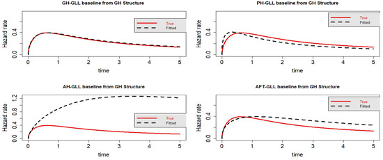
Figure 2. Estimated baseline hrfs with censoring proportion of $40\%$ and a sample size of $n=5000$. The dashed and solid curves indicate the estimated and true hrfs, accordingly. The data generated from a GH structure.

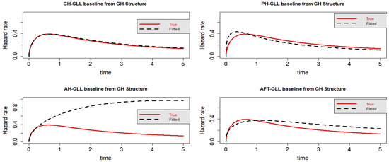
Figure 3. Estimated baseline hrfs with censoring proportion of $40\%$ and a sample size of n = 10,000. The dashed and solid curves indicate the estimated and true hrfs, accordingly. The data generated from a GH structure.

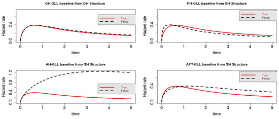
Figure 4. Estimated baseline hrfs with censoring proportion of $40\%$ and a sample size of n =10,000. The dashed and solid curves indicate the estimated and true hrfs, accordingly. The data generated from a GH structure.

Table 2. Simulation results from the GH model with $(k=0.625, \alpha =1.50$, and $\eta =1.0)$, covariates values for $({\beta }_1=0.75, 0.85, 0.95$, ${\beta }_2=0.35, 0.45, 0.55$) and $n=5000$ with about $20\%$ censoring. AIC, CAIC, and HQIC values for the competitive models.

Model	AIC	CAIC	HQIC
		$\mathbf{20}$% Censoring
GLL-GH Model	$9068.327$	$9068.705$	$9088.884$
GLL-AFT Model	$9202.449$	$9202.656$	$9216.154$
GLL-AH Model	$12,264.223$	$12,264.149$	$122,277.928$
GLL-PH Model	$9222.095$	$9222.307$	$9235.800$
		$\mathbf{40}$% censoring
GLL-GH Model	$5463.519$	$5463.598$	$5484.077$
GLL-AFT Model	$5505.834$	$5505.872$	$5519.540$
GLL-AH Model	$7424.734$	$7424.799$	$7438.440$
GLL-PH Model	$5548.739$	$5548.777$	$5562.444$

Table 3. Simulation results from the GH model with $(k=0.625, \alpha =1.50$, and $\eta =1.0)$, covariates values for $({\beta }_1=0.75, 0.85, 0.95$, ${\beta }_2=0.35, 0.45, 0.55$) and n = 10,000 with about $20\%$ censoring. AIC, CAIC, and HQIC values for the competitive models.

Model	AIC	CAIC	HQIC
		$\mathbf{20}$% Censoring
GLL-GH Model	17,567.525	175,672	17,589.491
GLL-AFT Model	17,843.352	17,843.429	17,857.996
GLL-AH Model	24,035.240	24,035.198	24,049.884
GLL-PH Model	17,818.738	17,818.184	17,833.382
		$\mathbf{40}$% censoring
GLL-GH Model	10,719.862	10,719.901	10,741.828
GLL-AFT Model	10,809.107	10,809.125	10,823.751
GLL-AH Model	14,662.298	14,662.330	14,676.942
GLL-PH Model	10,913.655	10,913.673	10,928.299

7.1.5. Results for Scenario 2

In Scenario 2, a simulation is generated using an AFT framework. The GLL-GH model and the true generated GLL-AFT model were all superior to the GLL-PH and GLL-AH models for the information criteria values, such as the AIC and CAIC values for Scenario 2. This demonstrates how the AFT model is a specific case of the GH framework. The generated model has the lowest AIC, CAIC, and HQIC values as would be predicted given that it is an AFT framework.

The GLL-GH model has the lowest AIC and CAIC values when the sample size and censoring fraction increase to n = 10,000 and $40\%$ censoring, respectively, as shown in Table 4 and Table 5. This shows that the GH structure performs better than its special cases when there is heavy censoring of the data. However, from the visual representations, it is clear that the GLL-GH and GLL-AFT models exhibit certain similarities and provide the best fit when compared to the other two rival models. We can, therefore, deduce from Scenario 2 that the AFT model is a sub-model of the GH model, as illustrated in Figure 5, Figure 6, Figure 7 and Figure 8.

Table 4. Simulation results from the AFT model with $(k=0.675, \alpha =1.50$, and $\eta =1.0)$, covariates values for $({\beta }_1=0.75, 0.85, 0.95$, $\left.{\beta }_2=0.75, 0.85, 0.95\right)$ and $n=5000$ with about $20\%$ and $40\%$ censoring. AIC, CAIC, and HQIC values for the competitive models.

	AIC	CAIC	HQIC
		$\mathbf{20}$% Censoring
GLL-AFT Model	9710.030	9710.583	9723.735
GLL-GH Model	9713.632	9714.807	9734.190
GLL-AH Model	12,766.930	12,766.869	12,780.635
GLL-PH Model	10,241.712	10,240.974	10,255.417
		$\mathbf{40}\%$ Censoring
GLL-AFT Model	6119.325	6119.367	6133.030
GLL-GH Model	6122.154	6122.246	6142.711
GLL-PH Model	6500.689	6500.739	6514.394
GLL-AH Model	8259.059	8249.154	8262.764

Table 5. Simulation results from the AFT model with $(k=0.675, \alpha =1.50$, and $\eta =1.0)$, covariates values for $({\beta }_1=0.75, 0.85, 0.95$, $\left.{\beta }_2=0.75, 0.85, 0.95\right)$ and n = 10,000 with about $20\%$ and $40\%$ censoring. AIC, CAIC, and HQIC values for the competitive models.

Model	AIC	CAIC	HQIC
		$\mathbf{20}$% Censoring
GLL-AFT Model	19,192.366	19,192.571	19,207.011
GLL-GH Model	19,195.876	19,196.313	19,217.842
GLL-AH Model	25,043.290	12,766.257	25,057.934
GLL-PH Model	20,201.167	20,200.269	20,215.811
		$\mathbf{40}\%$ censoring
GLL-AFT Model	12,214.303	12,214.324	12,228.947
GLL-GH Model	12,211.367	12,211.413	12,233.332
GLL-PH Model	13,036.386	13,036.410	13,051.030
GLL-AH Model	16,233.077	16,233.122	16,247.721

Figure 5. Estimated baseline hrfs with censoring proportion of $20\%$ and a sample size of $n=5000$. The dashed and solid curves indicate the estimated and true hrfs, accordingly. The data generated from an AFT structure.

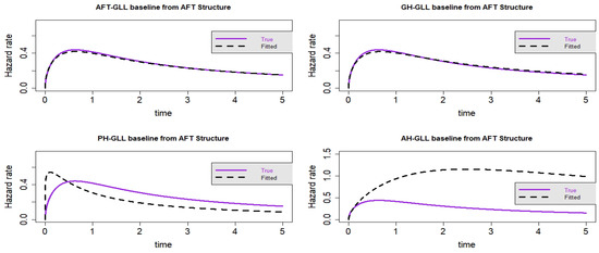
Figure 6. Estimated baseline hrfs with censoring proportion of $40\%$ and a sample size of $n=5000$. The dashed and solid curves indicate the estimated and true hrfs, accordingly. The data generated from an AFT structure.

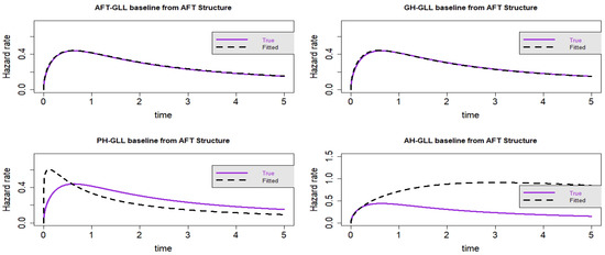
Figure 7. Estimated baseline hrfs with censoring proportion of $40\%$ and a sample size of n = 10,000. The dashed and solid curves indicate the estimated and true hrfs, accordingly. The data generated from an AFT structure.

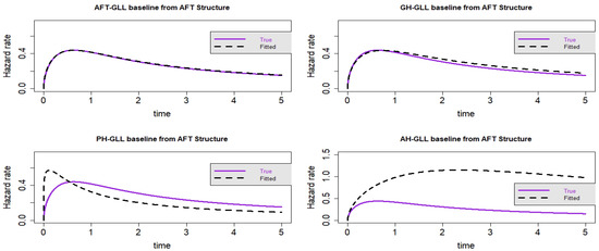
Figure 8. Estimated baseline hrfs with censoring proportion of $40\%$ and a sample size of n = 10,000. The dashed and solid curves indicate the estimated and true hrfs, accordingly. The data generated from an AFT structure.

7.1.6. Scenario 3 Results

In Scenario 3, a PH framework is used to generate simulation data. For information criteria values, such as the AIC and CAIC values for Scenario 3, the GLL-GH model and the true generated GLL-PH model were all superior to the GLL-AH and GLL-AFT models. This explains how the GH framework is used specifically in the PH model. Since the model created from the data were closed using the PH framework, the resultant GLL-PH model has the lowest AIC, CAIC, and HQIC values as would be expected.

As demonstrated in Table 6 and Table 7, the GLL-GH model’s AIC and CAIC values are comparable when the censoring fraction is increased to $40\%$. This demonstrates that when there is severe data censoring, the GH structure outperforms its special cases. However, it is obvious from the visual representations in Figure 9, Figure 10, Figure 11 and Figure 12 that the GLL-GH and GLL-PH models share several characteristics and offer the best fit when compared to the other two competing models. As we may infer from Scenario 3, the PH model is a sub-model of the GH model.

Table 6. Simulation results from the PH model with $(k=0.65, \alpha =1.50$, and $\eta =1.0)$, covariates values for $({\beta }_2=0.15, 0.25, 0.35$, $\left.{\beta }_1=0.0, 0.0, 0.0\right)$ and $n=5000$ with about $20\%$ and $40\%$ censoring. AIC, CAIC, and HQIC values for the competitive models.

Model	AIC	CAIC	HQIC
		$\mathbf{20}$% Censoring
GLL-PH Model	14,941.383	14,941.349	14,955.088
GLL-GH Model	14,947.070	14,946.997	14,967.627
GLL-AFT Model	15,037.394	15,037.361	15,051.100
GLL-AH Model	15,224.134	15,224.102	15,237.840
		$\mathbf{40}\%$ Censoring
GLL-PH Model	10,966.406	10,966.229	10,980.111
GLL-GH Model	10,966.497	10,966.116	10,987.054
GLL-AFT Model	11,038.579	11,038.415	11,052.284
GLL-AH Model	11,206.019	11,205.877	11,219.724

Table 7. Simulation results from the PH model with $(k=0.65, \alpha =1.50$, and $\eta =1.0)$, covariates values for $({\beta }_2=0.15, 0.25, 0.35$, $\left.{\beta }_1=0.0, 0.0, 0.0\right)$ and $n=10,000$ with about $20\%$ and $40\%$ censoring. AIC, CAIC, and HQIC values for the competitive models.

Model	AIC	CAIC	BIC
		$\mathbf{20}$% Censoring
GLL-PH Model	29,768.943	29,768.927	29,783.588
GLL-GH Model	29,772.045	29,772.008	29,794.011
GLL-AFT Model	29,969.703	29,969.686	29,984.345
GLL-AH Model	30,321.478	30,321.462	30,336.123
		$\mathbf{40}\%$ Censoring
GLL-PH Model	22,085.485	22,085.404	22,100.129
GLL-GH Model	22,088.317	22,088.143	22,110.283
GLL-AFT Model	22,219.687	22,219.611	22,234.331
GLL-AH Model	22,560.893	22,560.828	22,575.538

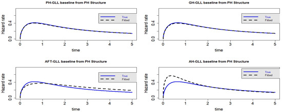
Figure 9. Estimated baseline hrfs with censoring proportion of $20\%$ and a sample size of $n=5000$. The dashed and solid curves indicate the estimated and true hrfs, accordingly. The data generated from a PH structure.

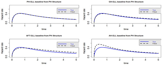
Figure 10. Estimated baseline hrfs with censoring proportion of $40\%$ and a sample size of $n=5000$. The dashed and solid curves indicate the estimated and true hrfs, accordingly. The data generated from a PH structure.

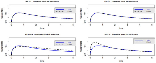
Figure 11. Estimated baseline hrfs with censoring proportion of $40\%$ and a sample size of n = 10,000. The dashed and solid curves indicate the estimated and true hrfs, accordingly. The data generated from a PH structure.

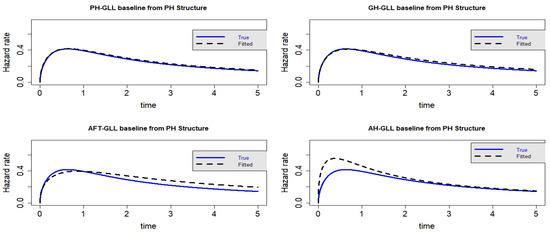
Figure 12. Estimated baseline hrfs with censoring proportion of $40\%$ and a sample size of n = 10,000. The dashed and solid curves indicate the estimated and true hrfs, accordingly. The data generated from a PH structure.

7.1.7. Scenario 4 Results

In the context of Scenario 4, some proximity can be accounted for by the visual representation in Figure 13, Figure 14, Figure 15 and Figure 16 of all the fitted models. Nevertheless, as anticipated, the GLL-GH and GLL-AH models outperform the two other rival models, the GLL-AFT and GLL-PH models. When compared to the other models, the GLL-GH model is the most similar to the actual created model, demonstrating that the GH framework is a general instance of the AH framework. As demonstrated in Table 8 and Table 9, the GLL-AH model has the lowest value for information criteria because it is the generated model from simulation data.

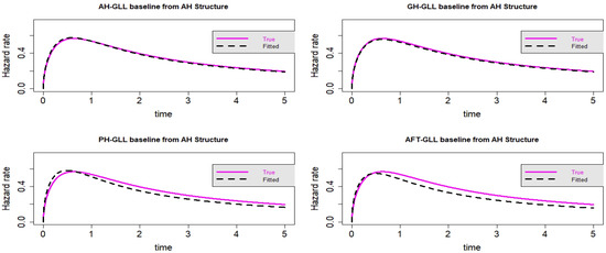
Figure 13. Estimated baseline hrfs with censoring proportion of $20\%$ and a sample size of $n=5000$. The dashed and solid curves indicate the estimated and true hrfs, accordingly. The data generated from an AH structure.

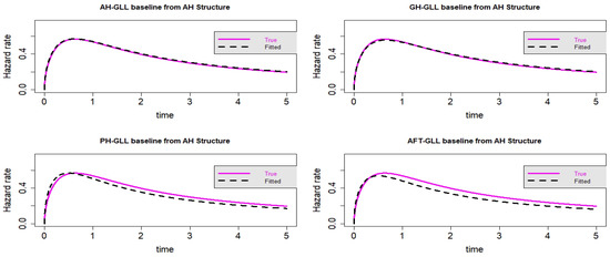
Figure 14. Estimated baseline hrfs with censoring proportion of $40\%$ and a sample size of $n=5000$. The dashed and solid curves indicate the estimated and true hrfs, accordingly. The data generated from an AH structure.

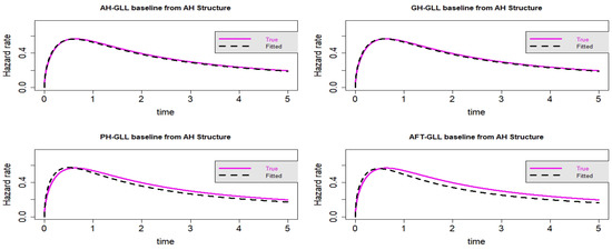
Figure 15. Estimated baseline hrfs with censoring proportion of $40\%$ and a sample size of n = 10,000. The dashed and solid curves indicate the estimated and true hrfs, accordingly. The data generated from an AH structure.

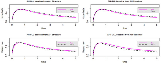
Figure 16. Estimated baseline hrfs with censoring proportion of $40\%$ and a sample size of n = 10,000. The dashed and solid curves indicate the estimated and true hrfs, accordingly. The data generated from an AH structure.

Table 8. Simulation results from the AH model with $(k=0.80, \alpha =1.50$, and $\eta =1.0)$, covariates values for $({\beta }_1=0.15, 0.25, 0.35$, $\left.{\beta }_2=0.0, 0.0, 0.0\right)$ and $n=5000$ with about $20\%$ and $40\%$ censoring. AIC, CAIC, and HQIC values for the competitive models.

Model	AIC	CAIC	HQIC
		$\mathbf{20}$% Censoring
GLL-AH Model	15,084.818	15,084.785	15,098.523
GLL-GH Model	15,086.243	15,086.172	15,106.801
GLL-PH Model	15,161.428	15,161.396	15,175.133
GLL-AFT Model	15,212.691	15,212.658	15,226.396
		$\mathbf{40}$% Censoring
GLL-AH Model	11,154.225	11,154.078	11,167.930
GLL-GH Model	11,156.478	11,156.161	11,177.035
GLL-PH Model	11,229.268	11,229.130	11,242.974
GLL-AFT Model	11,252.678	11,252.542	11,266.382

Table 9. Simulation results from the AH model with $(k=0.80, \alpha =1.50$, and $\eta =1.0)$, covariates values for $({\beta }_1=0.15, 0.25, 0.35$, $\left.{\beta }_2=0.0, 0.0, 0.0\right)$ and $n=10,000$ with about $20\%$ and $40\%$ censoring. AIC, CAIC, and HQIC values for the competitive models.

Model	AIC	CAIC	HQIC
		$\mathbf{20}$% Censoring
GLL-AFT Model	30,458.953	30,458.937	30,473.597
GLL-GH Model	30,463.451	30,463.416	30,485.416
GLL-AH Model	30,664.667	30,664.651	30,679.310
GLL-PH Model	30,741.659	30,741.644	30,756.303
		$\mathbf{40}\%$ Censoring
GLL-AFT Model	22,592.371	22,592.306	22,607.015
GLL-AFT Model	22,598.029	22,597.890	22,619.996
GLL-GH Model	22,776.538	22,776.477	22,791.182
GLL-AH Model	22,822.921	22,822.861	22,837.565

From the data in Table 2, Table 3, Table 4, Table 5, Table 6 and Table 7, the GH model may have a better performance, but it is hard to say that improvements for the GH model is significant. The GH model, as expected, has a nested structure with a versatile closed-form expression, making it more suitable for censored lifetime data analysis. Finally, the simulation results noted that the GH model has the ability to be a very valuable tractable parametric hazard-based model for sufficiently describing various types of lifetime data from various hazard rate shapes and censoring percent-ages, as well as a numerical tool for making comparisons between the three different approaches for hazard-based models, namely, the AH, PH, and AFT structures.

7.2. Simulation Study II: Performance Study

The Bayesian methodology of the proposed model is addressed in Simulation Study II. The aim of this analysis is to illustrate the Bayesian inferential properties of the estimators in the proposed model. In particular, we show how sample size and censoring percentages affect the proposed model’s Bayesian inferential properties.

7.2.1. Measures of Performance

The posterior mean, absolute bias (AB), mean square error (MSE), effective number of different simulations draws $\left(n_{eff}\right)$, coverage probability (CP), and potential scale reduction factor $\left(\widehat{R}\right)$ were used to evaluate the Bayesian inferential features of the proposed GH model.

The estimators’ bias is determined as follows:

$$Bias\left(\widehat{\theta }\right)=\frac{1}{N}\sum _{i=1}^N(\widehat{{\theta }_i}-\theta ).$$

(66)

The MSE is a useful indication of overall correctness and is computed as:

$$MSE\left(\widehat{\theta }\right)=\frac{1}{N}\sum _{i=1}^N{(\widehat{{\theta }_i}-\theta )}^2,$$

(67)

where $\theta =(\alpha ,\kappa ,\eta ,{\beta }^{\prime })$.

The following is a description of CP:

$$\mathrm{CP}=\widehat{\theta }\mp 1.96\times \mathrm{SE}\left(\widehat{\theta }\right).$$

(68)

According to Gelman et al. [50], the effective number of sample size simulation draws should be more than or equal to 400 in order to verify the convergence diagnostics of McMC simulations. The maximum permitted limit of $\left(\widehat{R}\right)$ should also be close to $1(\widehat{R}<$$1.10)$.

7.2.2. Posterior Analysis of Simulation Study II

In the simulation sets, we incorporated the proposed parametric GH model with the GLL baseline distribution to examine its Bayesian inferential characteristics. Each simulation set was utilized to estimate the suggested GH model with various censoring rates and sample sizes. Three parallel chains with 60,000 iterations each, plus additional 6000 for the burn-in time were utilized to approximate posterior distributions using JAGS software [51]. The chains were shortened further by storing every 10th draw to reduce auto-correlation in the sequences.

7.2.3. Simulation Results of Simulation Study II

Based on these findings reported in Table 10 and Table 11, we can infer that the estimators’ biases and MSE decrease with sample size, and that the estimators’ bias and MSE are also influenced by the censoring percentage, with greater censoring proportions increasing MSE and absolute bias (AB). The Gelman–Rubin diagnostic (potential scale reduction factor) and the number of efficiency sample size draws, on the other hand, illustrate that convergence has been reached. The estimators’ coverage probability was close to $95\%$.

Table 10. Results of the McMC simulation for Study II (Bayesian inference) under the GLL-GH framework with baseline hazard parameter values of $(\alpha =1.40, k=0.80$, and $\eta =1.20)$; covariate values of ${\beta }_1=(0.25, 0.35, 0.45),{\beta }_2=(0.55, 0.65, 0.75)$; sample size of 100; and two censoring proportions for rates of 20 and $40\%$.

True Value $\left(\widehat{\mathit{\theta }}\right)$	Posterior Mean	AB	MSE	CP	n-eff	$\widehat{\mathit{R}}$
			20% Censoring
${\beta }_{11}=0.25$	0.260	0.010	0.005	94.13	5232	1.002
${\beta }_{12}=0.35$	0.378	0.028	0.014	93.96	4313	1.002
${\beta }_{13}=0.45$	0.475	0.025	0.010	94.60	4717	1.000
${\beta }_{21}=0.55$	0.595	0.045	0.015	93.88	3987	1.000
${\beta }_{22}=0.65$	0.714	0.064	0.026	92.37	3243	1.000
${\beta }_{23}=0.75$	0.822	0.072	0.032	95.03	3456	1.000
$\alpha =1.40$	1.425	0.025	0.011	94.50	5404	1.001
$\kappa =0.80$	0.833	0.033	0.025	94.23	5039	1.002
$\eta =1.20$	1.224	0.024	0.021	95.67	4788	1.002
			30% Censoring
${\beta }_{11}=0.25$	0.292	0.042	0.007	92.47	5032	1.003
${\beta }_{12}=0.35$	0.386	0.036	0.015	92.55	4519	1.004
${\beta }_{13}=0.45$	0.483	0.033	0.012	93.41	4788	1.001
${\beta }_{21}=0.55$	0.606	0.056	0.018	94.69	3987	1.001
${\beta }_{22}=0.65$	0.720	0.070	0.023	96.82	3832	1.001
${\beta }_{23}=0.75$	0.831	0.081	0.033	94.45	4156	1.000
$\alpha =1.40$	1.436	0.036	0.013	96.32	5122	1.002
$\kappa =0.80$	0.847	0.047	0.028	91.60	5039	1.001
$\eta =1.20$	1.232	0.032	0.024	93.09	5188	1.001

Table 11. Results of the McMC simulation for Study II (Bayesian inference) under the GLL-GH framework with baseline hazard parameter values of $(\alpha =1.40, k=0.80$, and $\eta =1.20)$; covariate values of ${\beta }_1=(0.25, 0.35, 0.45),{\beta }_2=(0.55, 0.65, 0.75)$; sample size of 300; and two censoring proportions for rates of 20 and $40\%$.

True Value $\left(\widehat{\mathit{\theta }}\right)$	Posterior Mean	AB	MSE	CP	n-eff	$\widehat{\mathit{R}}$
			20% Censoring
${\beta }_{11}=0.25$	0.258	0.008	0.004	95.14	4898	1.000
${\beta }_{12}=0.35$	0.368	0.018	0.012	95.03	4020	1.000
${\beta }_{13}=0.45$	0.470	0.020	0.008	94.93	5676	1.000
${\beta }_{21}=0.55$	0.590	0.040	0.013	95.80	5413	1.000
${\beta }_{22}=0.65$	0.704	0.054	0.024	94.80	5213	1.000
${\beta }_{23}=0.75$	0.802	0.052	0.030	95.04	5093	1.000
$\alpha =1.40$	1.425	0.025	0.010	95.12	5003	1.000
$\kappa =0.80$	0.803	0.003	0.002	95.07	4937	1.000
$\eta =1.20$	1.204	0.004	0.003	94.92	4953	1.000
			30% Censoring
${\beta }_{11}=0.25$	0.292	0.042	0.006	94.00	5099	1.000
${\beta }_{12}=0.35$	0.386	0.036	0.014	95.25	5676	1.001
${\beta }_{13}=0.45$	0.483	0.033	0.011	94.763	55122	1.000
${\beta }_{21}=0.55$	0.606	0.321	0.013	95.43	3056	1.002
${\beta }_{22}=0.65$	0.720	0.70	0.020	95.55	3898	1.001
${\beta }_{23}=0.75$	0.831	0.081	0.031	94.34	4454	1.000
$\alpha =1.40$	1.436	0.036	0.012	96.32	4989	1.001
$\kappa =0.80$	0.847	0.047	0.026	95.00	5006	1.000
$\eta =1.20$	1.232	0.032	0.020	96.05	5012	1.001

8. Application

The most commonly used type of censored data in oncology studies is right-censored survival data. In these analyses, the time-to-event is commonly the time between survival and death. This section focuses on the use of parametric hazard-based regression models to reanalyze two real-world right-censored oncology datasets that have previously been addressed in the literature. The purpose of this study is to compare the parametric general hazard (GH) regression model to its special cases, which include the PH, AFT, and AH model frameworks, with the generalized log-logistic baseline. In the first of the two datasets, there are crossing survival curves, but there are no crossover survival curves in the second.

8.1. Colon Cancer Dataset

8.1.1. Data Description

In this section, we take a look at a genuine survival time data set for people with colon cancer that is openly accessible using the R package survival under the label of colon [52]. Initially, Laurie [53] described the study. Moertel [54] contains the main report. The final Moertel report’s dataset and this one are most similar [55]. Lin’s paper [56] made use of a version of the data with fewer follow-up times (1994). This colon cancer dataset has gained widespread use in the literature on survival analysis, and it is particularly simple to locate in research involving parametric hazard-based regression models.

This clinical trial’s experiment involved 1858 patients. These findings come from one of the earliest trials of adjuvant treatment for colon cancer that was successful. Levamisole is a low-toxicity drug formerly utilized to treat worm infestations in animals, while 5-FU is a chemotherapy drug that is moderately toxic (as these things go). Each individual has two records: one for recurrence and one for death.

The following variables were taken into account for each patient $(i=1,\dots ,1858)$:

i.

$t_i$: time until event or censoring;

ii.

status: censoring status ( $1=$ observed lifetime, $0=$ censored);

iii.

age: age of the patient in years;

iv.

surg: time from surgery to registration (1 = long, $0=$ short);

v.

etype: type of event $(1=$ recurrence, $2=$ death).

The total number of patients whose surgery takes a long time are 494 patients (26.59%), among whom $247(50\%)$ died. The Kaplan–Meier plot for the surgery variable is reported in Figure 17.

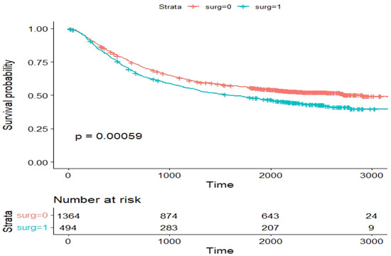
Figure 17. Kaplan–Meier survival plot for the variable surgery status ($1=long,0=short$).

8.1.2. Visual Representation of the Data

Analysis: The non-parametric plots for the survival time of colon cancer patients are reported in Figure 18. TTT plot for the survival time indicates an increasing hazard rate pattern.

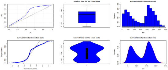
Figure 18. Non-parametric plots for the survival time data of colon cancer patients.

8.2. Classical Analysis

For the proposed GH model and its sub-models, including the $\mathrm{PH},\mathrm{AH}$, and AFT models with GLL baseline distribution, the MLE estimates for baseline distribution parameters and regression coefficients are provided in Table 12, and the estimated hrfs for the competitive models are given in Figure 19.

Table 12. Results from the fitted parametric hazard-based regression models to colon cancer dataset.

Models	Parameter(s)	Estimate	SE	Z-Value	p-Value	L-95%	U-95%
GLL-GH	${\beta }_{11}$	0.065	0.038	0.593	0.553	−0.053	0.171
	${\beta }_{12}$	−0.171	0.129	−1.331	0.183	−0.423	0.081
	${\beta }_{13}$	−1.549	0.118	−13.185	<0.001	−1.780	−1.139
	${\beta }_{21}$	0.012	0.039	0.316	0.752	−0.065	0.090
	${\beta }_{22}$	0.161	0.087	1.850	0.064	−0.010	0.331
	${\beta }_{23}$	−0.890	0.072	−12.339	<0.001	−1.032	−0.749
	$\alpha$	1.938	0.127	8.932	<0.001	1.690	2.187
	$\kappa$	0.009	0.001	15.290	<0.001	0.007	0.011
	$\eta$	0.039	0.006	6.697	<0.001	0.028	0.187
GLL-AFT	${\beta }_1$	0.023	0.038	0.593	0.553	−0.053	0.098
	${\beta }_2$	0.100	0.089	1.131	0.258	−0.074	0.274
	${\beta }_3$	−0.970	0.058	−16.864	<0.001	−1.083	−0.857
	$\alpha$	2.381	0.139	17.175	<0.001	2.161	2.653
	$\kappa$	0.008	0.001	10.986	<0.001	0.011	0.009
	$\eta$	0.019	0.002	11.213	<0.001	0.042	0.022
GLL-PH	${\beta }_1$	−0.064	0.033	−1.936	0.043	−0.129	0.001
	${\beta }_2$	0.167	0.072	2.323	0.020	0.026	0.309
	${\beta }_3$	−0.518	0.052	−9.978	<0.001	−0.620	−0.417
	$\alpha$	1.938	0.127	8.932	<0.001	1.690	2.187
	$\kappa$	0.009	0.001	15.290	<0.001	0.007	0.011
	$\eta$	0.039	0.006	6.697	<0.001	0.028	0.187
GLL-AH	${\beta }_1$	0.029	0.047	0.620	0.535	−0.062	0.120
	${\beta }_2$	−0.464	0.108	−4.288	<0.001	−0.676	−0.252
	${\beta }_3$	−1.139	0.090	−12.648	<0.001	−1.315	−0.962
	$\alpha$	2.113	0.084	25.226	<0.001	2.161	2.277
	$\kappa$	0.004	0.000	17.158	<0.001	0.011	0.005
	$\eta$	0.024	0.003	9.495	<0.001	0.042	0.029

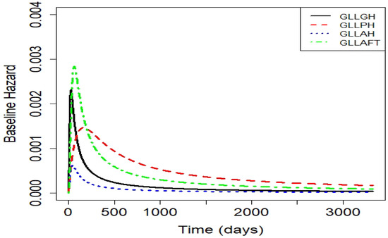
Figure 19. Estimated hazards for the competitive models of the colon cancer dataset.

8.3. Frequentist Model Comparison

We take into account the AIC, CAIC, and HQIC when comparing frequentist models. The proposed GH model is the most effective model when compared to its rival models, according to the estimates of the AIC, CAIC, and HQIC in Table 13.

Table 13. Results for some frequentist information criteria for the hazard-based regression models.

Model	AIC	CAIC	HQIC
GH	16,276.09	16,276.07	16,294.43
PH	16,415.50	16,415.50	16,427.74
AH	16,384.96	16,384.94	16,397.94
AFT	16,294.36	16,294.35	16,306.58

Likelihood Ratio Test

To form a comprehensive statistical inference about a model, it is necessary to lower the number of parameters and assess how this impacts the model’s ability to match the data. The likelihood ratio test (LRT) is used to compare the GH model to its sub-models, which include the PH, AFT, and AH hazard-based regression models. The LRT statistic and its accompanying p-values in Table 14 show that the GH model fits better than its sub-models for the colon cancer lifetime dataset.

Table 14. LRT test for the GH model and its sub-models.

Model	Hypothesis	LRT	p-Value
GH vs. PH	$H_0:{\beta }_2=0, H_1:H_0$ is false,	145.424	<0.001
GH vs. AH	$H_0:{\beta }_1=0, H_1:H_0$ is false,	114.863	<0.001
GH vs. AFT	$H_0:{\beta }_1={\beta }_2, H_1:H_0$ is false,	24.268	<0.001

8.4. Bayesian Analysis

We used Bayesian analysis to compare the proposed GLL-GH model with its competing models, such as the GLL-PH, GLL-AH, and GLL-AFT models. The baseline distribution parameters $\alpha \sim G\left(a_1,b_1\right),\eta \sim G\left(a_2,b_2\right)$, and $k\sim G\left(a_3,b_3\right)$ with hyper-parameter values $\left(a_1=b_1=a_2=b_2=a_3=b_3=10\right)$ are assumed to have separate gamma priors that are independent and non-informative normal prior with a value of $N(0,100)$ for ${\beta }^{\prime }s$ (regression coefficients). Rstan package was utilized for our analysis [57].

8.4.1. Numerical Summary

In this section, we used the McMC sample of posterior properties for the generalized log-logistic general hazard (GLL-GH) model and its special cases, including the GLL-PH, GLL-AH, and GLL-AFT models in Table 15, to examine several posterior properties of interest and their numerical values.

Table 15. Results for the posterior properties of the competitive models.

Models	Par (s)	Estimate	SE	SD	2.5%	Medium	97.5%	${\mathit{N}}_{\mathbf{eff}}$	$\widehat{\mathit{R}}$
GLL-GH	${\beta }_{11}$	0.086	0.001	0.	−0.016	0.087	0.187	4013	1.001
	${\beta }_{12}$	−0.172	0.002	0.122	−0.412	−0.174	0.067	4049	1.001
	${\beta }_{13}$	−1.500	0.003	0.129	−1.752	−1.497	−1.264	2174	1.004
	${\beta }_{21}$	0.009	0.001	0.040	−0.070	0.009	0.086	4772	1.000
	${\beta }_{22}$	0.161	0.001	0.087	−0.004	0.158	0.333	4151	1.001
	${\beta }_{23}$	−0.925	0.002	0.088	−1.097	−0.925	−0.756	2410	1.003
	$\alpha$	2.166	0.002	0.138	1.909	2.161	2.449	4951	1.001
	$\kappa$	0.011	0.000	0.002	0.008	0.011	0.016	2174	1.004
	$\eta$	0.044	0.000	0.009	0.029	0.042	0.064	2016	1.004
GLL-AFT	${\beta }_1$	0.021	0.001	0.038	−0.057	0.021	0.095	5059	1.001
	${\beta }_2$	0.101	0.001	0.089	−0.073	0.100	0.271	5069	1.000
	${\beta }_3$	−1.012	0.002	0.081	−1.168	−1.012	−0.855	2685	1.001
	$\alpha$	2.282	0.002	0.134	2.033	2.277	2.554	4304	1.000
	$\kappa$	0.008	0.000	0.001	0.006	0.008	0.011	2426	1.001
	$\eta$	0.020	0.000	0.003	0.015	0.020	0.027	2470	1.001
GLL-PH	${\beta }_1$	−0.029	0.000	0.034	−0.096	−0.029	0.039	5944	1.000
	${\beta }_2$	0.238	0.001	0.071	0.099	0.238	0.374	5490	1.000
	${\beta }_3$	−0.245	0.001	0.066	−0.374	−0.245	−0.116	4336	1.000
	$\alpha$	1.997	0.002	0.000	−1.767	1.993	2.242	3623	1.001
	$\kappa$	0.002	0.000	0.122	0.002	0.002	0.002	2912	1.002
	$\eta$	0.004	0.000	0.000	0.004	0.004	0.005	3235	1.001
GLL-AH	${\beta }_1$	0.071	0.001	0.043	−0.013	0.072	0.157	5046	1.000
	${\beta }_2$	−0.283	0.001	0.098	−0.479	−0.282	−0.094	4320	1.000
	${\beta }_3$	−0.744	0.002	0.096	−0.932	−0.744	−0.554	3425	1.001
	$\alpha$	2.218	0.002	0.132	1.970	2.216	2.487	3258	1.000
	$\kappa$	0.003	0.000	0.000	0.003	0.003	0.004	2728	1.001
	$\eta$	0.014	0.000	0.002	0.010	0.014	0.018	2904	1.001

8.4.2. Visual Summary

Figure 20, Figure 21, Figure 22, Figure 23, Figure 24, Figure 25, Figure 26 and Figure 27 provide the trace and autocorrelation (AC) plots for the baseline distribution parameters and regression coefficients of the proposed GH model and its sub-models, indicating convergence of the chains.

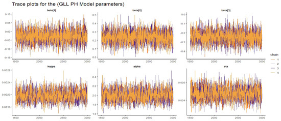
Figure 20. Trace plots for the GLL-PH model parameters.

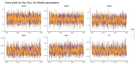
Figure 21. Trace plots for the GLL-AH model parameters.

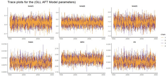
Figure 22. Trace plots for the GLL-AFT model parameters.

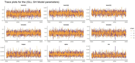
Figure 23. Trace plots for the GLL-GH model parameters.

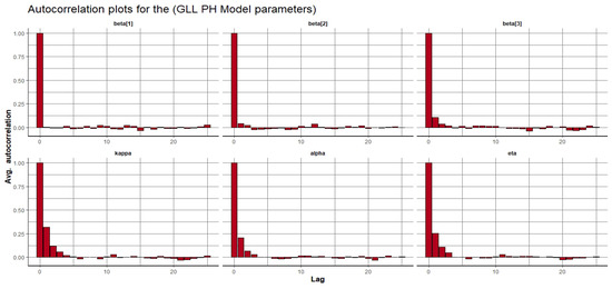
Figure 24. Autocorrelation plots for the GLL-PH model parameters.

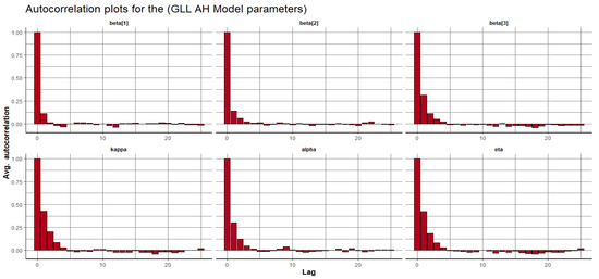
Figure 25. Autocorrelation plots for the GLL-AH model parameters.

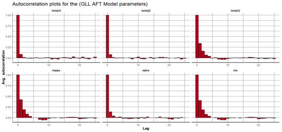
Figure 26. Autocorrelation plots for the GLL-AFT model parameters.

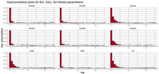
Figure 27. Autocorrelation plots for the GLL-GH model parameters.

8.4.3. McMC Convergence Diagnostics

We applied both numerical and visual methods to evaluate the convergence of the McMC algorithm for the proposed models and their special cases. As can be seen from the summary results in the above table, the McMC algorithm HMC-NUTS has converged to the joint posterior distribution because the potential scale reduction factor $\widehat{R}$ is 1, the effective sample size $\left(n_{eff}\right)$ is greater than 400, and the Monte Carlo error (SE) is less than $5\%$ of the posterior standard deviations for all of the parameters.

Visually assessing convergence is often done using autocorrelation and trace graphs [58]. Figure 20, Figure 21, Figure 22 and Figure 23 trace plot displays a stationary pattern fluctuating within a band, demonstrating the convergence of the McMC algorithm. Figure 24, Figure 25, Figure 26 and Figure 27 autocorrelation plot demonstrates how autocorrelation rapidly decreases to zero as the period of lag increases, indicating good mixing and the convergence of the algorithm to the desired posterior distribution.

8.4.4. Bayesian Model Selection

We implemented two information criteria, Watanabe AIC (WAIC), proposed by [59], for the Bayesian model comparison, and the Vehtari et al. [60] proposed Leave-one-out information criteriON (LOOIC). A model may be said to be best suited if it has the lowest WAIC and LOOIC values for both information criteria. In addition to Stan fitting, posterior predictive check (PPC) and determining WAIC and LOOIC are performed using the R package loo [61]. Table 16, below, shows that when compared to its rival models, the GLL-GH model is the most effective.

Table 16. Bayesian model comparison for the GLL-GH and its special cases.

Model	WAIC	LOOIC
GH	16,274.00	16,274.01
PH	16,360.20	16,360.21
AH	16,345.80	16,345.90
AFT	16,295.75	16,295.80

9. Conclusions

The PH, AFT, and AH models are three ways to develop hazard-based regression models for survival data. Because of the relative risk interpretation of the regression coefficients and the existence of a semi-parametric PH model that is robust against the distributional assumption of the survival time, PH models are particularly popular in clinical trials and oncology investigations. The goal of this study was to generalize the hazard-based regression models stated above to include both time-independent and time-dependent covariates in a single model, dubbed the GH model. The main goal of this model is to distinguish scenarios in which covariates have a time-independent or time-dependent effect on the hazard rate when modelling survival data, with a focus on parametric models.

In general, if the underlying distributional assumption is relatively true, a para-metric model is chosen in statistical data analysis. In survival data analysis, parametric hazard-based regression models can provide more accurate estimations of the regression coefficients than semi-parametric hazard-based regression models (Collet, 2015). Other essential values, such as quantiles, the hrf, and survival probabilities, can also be easily estimated using parametric models. It is worth noting that the hazard function is a key part of the time course of a disease process, therefore it is a focus of many clinical investigations.

The Cox PH model does practically all of the modelling of censored survival data. The non-proportional hazard models, such as the AFT and AH models, are chosen as an alternative once the proportionality assumption is discarded. On the other hand, AFT and AH models can only include covariates with time-dependent and non-proportional effects on the hazard overtime, whereas a PH model can only have time-independent and proportional effects. The GH model established in this work can accept a variety of covariates, some of which may have time-independent and proportional impacts on the hazard value, while others may have time-dependent and non-proportional effects. Another advantage of the model is that it may be used to predict when survival and hazard rates will cross.

A detailed simulation study was conducted to evaluate the performance of the suggested GH model. The findings show that the GH model produces better outcomes, with fewer biases detected for the majority of parameters. The layered structure of the GH model in comparison to the PH, AFT, and AH models for a broad regression setting containing various covariates prevalent in cancer epidemiology studies was further explored using simulated datasets. The results demonstrate the GH model’s nested structure and tractability once more. Following the simulation study, this paper shows a real-world data application with right-censored cancer datasets from a patient clinical trial. When the information criterion used in this study was evaluated, the GLL-GH model outperformed the GLL-PH, GLL-AH, and GLL-AFT models.

In future research, more complicated GH models may be investigated in order to modify the GH model and make it more tractable for modelling censored survival data. By expanding the GH model, other common hazard-based regression models such as the PO and YP models can be incorporated. Other potential research projects include the creation of residual analysis tools and diagnostic metrics to assess the suggested models’ goodness of fit. We want to extend the proposed GH model in future work to accommodate interval-censored data, as well as survival data with competing hazards and cure fractions.

References

- Zhou, H.; Hanson, T. Bayesian spatial survival models. In Nonparametric Bayesian Inference in Biostatistics; Springer: Berlin, Germany, 2015; pp. 215–246. [Google Scholar]
- Alvares, D.; Lázaro, E.; Gómez-Rubio, V.; Armero, C. Bayesian survival analysis with BUGS. Stat. Med. 2021, 40, 2975–3020. [Google Scholar] [CrossRef] [PubMed]
- Rubio, F.J.; Remontet, L.; Jewell, N.P.; Belot, A. On a general structure for hazard-based regression models: An application to population-based cancer research. Stat. Methods Med. Res. 2019, 28, 2404–2417. [Google Scholar] [CrossRef] [PubMed]
- Demarqui, F.N.; Mayrink, V.D. Yang and Prentice model with piecewise exponential baseline distribution for modeling lifetime data with crossing survival curves. Braz. J. Probab. Stat. 2021, 35, 172–186. [Google Scholar] [CrossRef]
- Rubio, F.J.; Rachet, B.; Giorgi, R.; Maringe, C.; Belot, A. On models for the estimation of the excess mortality hazard in case of insufficiently stratified life tables. Biostatistics 2021, 22, 51–67. [Google Scholar] [CrossRef]
- Cox, D.R. Regression models and life-tables. J. R. Stat. Soc. Ser. B (Methodol.) 1972, 34, 187–202. [Google Scholar] [CrossRef]
- Lawless, J.F. Statistical Models and Methods for Lifetime Data; John Wiley & Sons: Hoboken, NJ, USA, 2011. [Google Scholar]
- Hjort, N.L. On inference in parametric survival data models. Int. Stat. Rev. Int. Stat. 1992, 60, 355–387. [Google Scholar] [CrossRef]
- Mudholkar, G.S.; Hutson, A.D. The exponentiated Weibull family: Some properties and a flood data application. Commun.-Stat.-Theory Methods 1996, 25, 3059–3083. [Google Scholar] [CrossRef]
- Chesneau, C.; Jamal, F. The sine Kumaraswamy-G family of distributions. J. Math. Ext. 2020, 15. [Google Scholar]
- Alkhairy, I.; Nagy, M.; Muse, A.H.; Hussam, E. The Arctan-X family of distributions: Properties, simulation, and applications to actuarial sciences. Complexity 2021, 2021, 4689010. [Google Scholar] [CrossRef]
- Mahmood, Z.; M Jawa, T.; Sayed-Ahmed, N.; Khalil, E.; Muse, A.H.; Tolba, A.H. An Extended Cosine Generalized Family of Distributions for Reliability Modeling: Characteristics and Applications with Simulation Study. Math. Probl. Eng. 2022, 2022, 3634698. [Google Scholar] [CrossRef]
- Souza, L.; de Oliveira, W.R.; de Brito, C.C.R.; Chesneau, C.; Fernandes, R.; Ferreira, T.A. Sec-G class of distributions: Properties and applications. Symmetry 2022, 14, 299. [Google Scholar] [CrossRef]
- Muse, A.H.; Tolba, A.H.; Fayad, E.; Abu Ali, O.A.; Nagy, M.; Yusuf, M. Modelling the COVID-19 mortality rate with a new versatile modification of the log-logistic distribution. Comput. Intell. Neurosci. 2021, 2021, 8640794. [Google Scholar] [CrossRef] [PubMed]
- Muse, A.H.; Mwalili, S.; Ngesa, O.; Almalki, S.J.; Abd-Elmougod, G.A. Bayesian and classical inference for the generalized log-logistic distribution with applications to survival data. Comput. Intell. Neurosci. 2021, 2021, 5820435. [Google Scholar] [CrossRef]
- Kalbfleisch, J.D.; Prentice, R.L. The Statistical Analysis of Failure Time Data; John Wiley & Sons: Hoboken, NJ, USA, 2011. [Google Scholar]
- Demarqui, F.N.; Mayrink, V.D.; Ghosh, S.K. An Unified Semiparametric Approach to Model Lifetime Data with Crossing Survival Curves. arXiv 2019, arXiv:1910.04475. [Google Scholar]
- Chen, Y.Q.; Wang, M.C. Analysis of accelerated hazards models. J. Am. Stat. Assoc. 2000, 95, 608–618. [Google Scholar] [CrossRef]
- Wang, K.; Ye, X.; Ma, J. An empirical analysis of post-work grocery shopping activity duration using modified accelerated failure time model to differentiate time-dependent and time-independent covariates. PLoS ONE 2018, 13, e0207810. [Google Scholar] [CrossRef] [PubMed]
- Ciampi, A.; Etezadi-Amoli, J. A general model for testing the proportional hazards and the accelerated failure time hypotheses in the analysis of censored survival data with covariates. Commun.-Stat.-Theory Methods 1985, 14, 651–667. [Google Scholar] [CrossRef]
- Etezadi-Amoli, J.; Ciampi, A. Extended hazard regression for censored survival data with covariates: A spline approximation for the baseline hazard function. Biometrics 1987, 181–192. [Google Scholar] [CrossRef]
- Louzada-Neto, F. Extended hazard regression model for reliability and survival analysis. Lifetime Data Anal. 1997, 3, 367–381. [Google Scholar] [CrossRef]
- Louzada-Neto, F. Bayesian Analysis for Hazard Models with Non-constant Shape Parameter. Comput. Stat. 2001, 16, 243–254. [Google Scholar] [CrossRef]
- Chen, Y.Q.; Jewell, N.P. On a general class of semiparametric hazards regression models. Biometrika 2001, 88, 687–702. [Google Scholar] [CrossRef]
- Elsayed, E.A.; Liao, H.; Wang, X. An extended linear hazard regression model with application to time-dependent dielectric breakdown of thermal oxides. Lie Trans. 2006, 38, 329–340. [Google Scholar] [CrossRef]
- Tong, X.; Zhu, L.; Leng, C.; Leisenring, W.; Robison, L.L. A general semiparametric hazards regression model: Efficient estimation and structure selection. Stat. Med. 2013, 32, 4980–4994. [Google Scholar] [CrossRef] [PubMed]
- Li, L.; Hanson, T.; Zhang, J. Spatial extended hazard model with application to prostate cancer survival. Biometrics 2015, 71, 313–322. [Google Scholar] [CrossRef] [PubMed]
- Rubio Alvarez, F.J.; Drikvandi, R. MEGH: A parametric class of general hazard models for clustered survival data. Stat. Methods Med. Res. 2022, 31. [Google Scholar] [CrossRef]
- Muse, A.H.; Ngesa, O.; Mwalili, S.; Alshanbari, H.M.; El-Bagoury, A.A.H. A Flexible Bayesian Parametric Proportional Hazard Model: Simulation and Applications to Right-Censored Healthcare Data. J. Healthc. Eng. 2022, 2022, 2051642. [Google Scholar] [CrossRef] [PubMed]
- Rezaei, S.; Hashami, S.; Najjar, L. Extended exponential geometric proportional hazard model. Ann. Data Sci. 2014, 1, 173–189. [Google Scholar] [CrossRef][Green Version]
- Muse, A.H.; Mwalili, S.; Ngesa, O.; Alshanbari, H.M.; Khosa, S.K.; Hussam, E. Bayesian and frequentist approach for the generalized log-logistic accelerated failure time model with applications to larynx-cancer patients. Alex. Eng. J. 2022, 61, 7953–7978. [Google Scholar] [CrossRef]
- Co, C.A.T. Investigating the Use of the Accelerated Hazards Model for Survival Analysis. Master’s Thesis, Simon Fraser University, Burnaby, BC, Canada, 2010. [Google Scholar]
- Qing Chen, Y. Accelerated hazards regression model and its adequacy for censored survival data. Biometrics 2001, 57, 853–860. [Google Scholar] [CrossRef]
- Zhang, J.; Peng, Y. Crossing hazard functions in common survival models. Stat. Probab. Lett. 2009, 79, 2124–2130. [Google Scholar] [CrossRef] [PubMed]
- Bennett, S. Analysis of survival data by the proportional odds model. Stat. Med. 1983, 2, 273–277. [Google Scholar] [CrossRef] [PubMed]
- Tahir, M.; Mansoor, M.; Zubair, M.; Hamedani, G. McDonald log-logistic distribution with an application to breast cancer data. J. Stat. Theory Appl. 2014, 13, 65–82. [Google Scholar] [CrossRef]
- Mendoza, N.V.; Ortega, E.M.; Cordeiro, G.M. The exponentiated-log-logistic geometric distribution: Dual activation. Commun.-Stat.-Theory Methods 2016, 45, 3838–3859. [Google Scholar] [CrossRef]
- Muse, A.H.; Mwalili, S.M.; Ngesa, O. On the log-logistic distribution and its generalizations: A survey. Int. J. Stat. Probab. 2021, 10, 93. [Google Scholar]
- Singh, K.P.; Lee, C.M.S.; George, E.O. On Generalized Log-Logistic Model for Censored Survival Data. Biom. J. 1988, 30, 843–850. [Google Scholar] [CrossRef]
- Al-Aziz, S.N.; Muse, A.H.; Jawad, T.M.; Sayed-Ahmed, N.; Aldallal, R.; Yusuf, M. Bayesian inference in a generalized log-logistic proportional hazards model for the analysis of competing risk data: An application to stem-cell transplanted patients data. Alex. Eng. J. 2022, 61, 13035–13050. [Google Scholar] [CrossRef]
- Khan, S.A.; Khosa, S.K. Generalized log-logistic proportional hazard model with applications in survival analysis. J. Stat. Distrib. Appl. 2016, 3, 16. [Google Scholar] [CrossRef]
- Muse, A.H.; Mwalili, S.; Ngesa, O.; Kilai, M. AHSurv: An R Package for Flexible Parametric Accelerated Hazards (AH) Regression Models. 2022. Available online: https://cran.r-project.org/web/packages/AHSurv/index.html (accessed on 18 September 2022).
- Muse, A.H.; Mwalili, S.; Ngesa, O.; Chesneau, C. AmoudSurv: An R Package for Tractable Parametric Odds-Based Regression Models. 2022. Available online: https://cran.r-project.org/web/packages/AmoudSurv/index.html (accessed on 18 September 2022).
- Khan, S.A.; Basharat, N. Accelerated failure time models for recurrent event data analysis and joint modeling. Comput. Stat. 2022, 37, 1569–1597. [Google Scholar] [CrossRef]
- R Core Team. R: A Language and Environment for Statistical Computing; R Core Team: Vienna, Austria, 2013. [Google Scholar]
- Bender, R.; Augustin, T.; Blettner, M. Generating survival times to simulate Cox proportional hazards models. Stat. Med. 2005, 24, 1713–1723. [Google Scholar] [CrossRef]
- Leemis, L.M.; Shih, L.H.; Reynertson, K. Variate generation for accelerated life and proportional hazards models with time dependent covariates. Stat. Probab. Lett. 1990, 10, 335–339. [Google Scholar] [CrossRef]
- Austin, P.C. Generating survival times to simulate Cox proportional hazards models with time-varying covariates. Stat. Med. 2012, 31, 3946–3958. [Google Scholar] [CrossRef]
- Rubio, F.J.; Alvares, D.; Redondo-Sanchez, D.; Marcos-Gragera, R.; Sánchez, M.J.; Luque-Fernandez, M.A. Bayesian variable selection and survival modeling: Assessing the Most important comorbidities that impact lung and colorectal cancer survival in Spain. BMC Med. Res. Methodol. 2022, 22, 95. [Google Scholar] [CrossRef] [PubMed]
- Gelman, A.; Carlin, J.B.; Stern, H.S.; Rubin, D.B. Bayesian Data Analysis; Chapman and Hall/CRC: Boca Raton, FL, USA, 1995. [Google Scholar]
- Denwood, M.J. runjags: An R package providing interface utilities, model templates, parallel computing methods and additional distributions for MCMC models in JAGS. J. Stat. Softw. 2016, 71, 1–25. [Google Scholar] [CrossRef]
- Therneau, T.; Lumley, T. R Survival Package; R Core Team: Vienna, Austria, 2013. [Google Scholar]
- Laurie, J.A.; Moertel, C.G.; Fleming, T.R.; Wieand, H.S.; Leigh, J.E.; Rubin, J.; McCormack, G.W.; Gerstner, J.B.; Krook, J.E.; Malliard, J. Surgical adjuvant therapy of large-bowel carcinoma: An evaluation of levamisole and the combination of levamisole and fluorouracil. The North Central Cancer Treatment Group and the Mayo Clinic. J. Clin. Oncol. 1989, 7, 1447–1456. [Google Scholar] [CrossRef]
- Moertel, C.G.; Fleming, T.R.; Macdonald, J.S.; Haller, D.G.; Laurie, J.A.; Goodman, P.J.; Ungerleider, J.S.; Emerson, W.A.; Tormey, D.C.; Glick, J.H.; et al. Levamisole and fluorouracil for adjuvant therapy of resected colon carcinoma. N. Engl. J. Med. 1990, 322, 352–358. [Google Scholar] [CrossRef] [PubMed]
- Moertel, C.G.; Fleming, T.R.; Macdonald, J.S.; Haller, D.G.; Laurie, J.A.; Tangen, C.M.; Ungerleider, J.S.; Emerson, W.A.; Tormey, D.C.; Glick, J.H.; et al. Fluorouracil plus levamisole as effective adjuvant therapy after resection of stage III colon carcinoma: A final report. Ann. Intern. Med. 1995, 122, 321–326. [Google Scholar] [CrossRef]
- Lin, D. Cox regression analysis of multivariate failure time data: The marginal approach. Stat. Med. 1994, 13, 2233–2247. [Google Scholar] [CrossRef] [PubMed]
- Carpenter, B.; Gelman, A.; Hoffman, M.D.; Lee, D.; Goodrich, B.; Betancourt, M.; Brubaker, M.; Guo, J.; Li, P.; Riddell, A. Stan: A probabilistic programming language. J. Stat. Softw. 2017, 76. [Google Scholar] [CrossRef]
- Ashraf-Ul-Alam, M.; Khan, A.A. Generalized Topp-Leone-Weibull AFT Modelling: A Bayesian Analysis with MCMC Tools Using R and Stan. Austrian J. Stat. 2021, 50, 52–76. [Google Scholar] [CrossRef]
- Watanabe, S. A widely applicable Bayesian information criterion. J. Mach. Learn. Res. 2013, 14, 867–897. [Google Scholar]
- Vehtari, A.; Gelman, A.; Gabry, J. Practical Bayesian model evaluation using leave-one-out cross-validation and WAIC. Stat. Comput. 2017, 27, 1413–1432. [Google Scholar] [CrossRef]
- Vehtari, A.; Gelman, A.; Gabry, J.; Yao, Y. Package ‘loo’. Efficient Leave-One-Out Cross-Validation and WAIC for Bayesian Models. 2021. Available online: https://cran.r-project.org/web/packages/loo/index.html (accessed on 18 September 2022).
Publisher’s Note: MDPI stays neutral with regard to jurisdictional claims in published maps and institutional affiliations. |
© 2022 by the authors. Licensee MDPI, Basel, Switzerland. This article is an open access article distributed under the terms and conditions of the Creative Commons Attribution (CC BY) license (https://creativecommons.org/licenses/by/4.0/).