Retrial BMAP/PH/N Queueing System with a Threshold-Dependent Inter-Retrial Time Distribution

Abstract

In this paper, we study a multi-server queueing system with retrials and an infinite orbit. The arrival of primary customers is described by a batch Markovian arrival process ($BMAP$), and the service times have a phase-type ($PH$) distribution. Previously, in the literature, such a system was mainly considered under the strict assumption that the intervals between the repeated attempts from the orbit have an exponential distribution. Only a few publications dealt with retrial queueing systems with non-exponential inter-retrial times. These publications assumed either the rate of retrials is constant regardless of the number of customers in the orbit or this rate is constant when the number of orbital customers exceeds a certain threshold. Such assumptions essentially simplify the mathematical analysis of the system, but do not reflect the nature of the majority of real-life retrial processes. The main feature of the model under study is that we considered the classical retrial strategy under which the retrial rate is proportional to the number of orbital customers. However, in this case, the assumption of the non-exponential distribution of inter-retrial times leads to insurmountable computational difficulties. To overcome these difficulties, we supposed that inter-retrial times have a phase-type distribution if the number of customers in the orbit is less than or equal to some non-negative integer (threshold) and have an exponential distribution in the contrary case. By appropriately choosing the threshold, one can obtain a sufficiently accurate approximation of the system with a $PH$ distribution of the inter-retrial times. Thus, the model under study takes into account the realistic nature of the retrial process and, at the same time, does not resort to restrictions such as a constant retrial rate or to rough truncation methods often applied to the analysis of retrial queueing systems with an infinite orbit. We describe the behavior of the system by a multi-dimensional Markov chain, derive the stability condition, and calculate the steady-state distribution and the main performance indicators of the system. We made sure numerically that there was a reasonable value of the threshold under which our model can be served as a good approximation of the $BMAP/PH/N$ queueing system with the $PH$ distribution of inter-retrial times. We also numerically compared the system under consideration with the corresponding queueing system having exponentially distributed inter-retrial times and saw that the latter is a poor approximation of the system with the $PH$ distribution of inter-retrial times. We present a number of illustrative numerical examples to analyze the behavior of the system performance indicators depending on the system parameters, the variance of inter-retrial times, and the correlation in the input flow.

1. Introduction

When modeling the operation of telecommunication networks, it is necessary to take into account a large number of objective and subjective factors. These are: (a) the complex nature of information flows, which can have a large spread in the values of the intervals between customers and be correlated; (b) the phenomenon of retrials; (c) the more complex nature of the distribution of intervals between retrials (in comparison with the well-studied exponential distribution). The presence of retrials significantly complicates the mathematical analysis of the system in comparison with queueing systems with waiting room or with losses. At the same time, retrial queueing systems find great interest among researchers in the field of telecommunications and queueing theory since they adequately describe the operation of versatile communication networks, including cellular mobile networks for various purposes, as well as various contact centers, etc. In the literature, one can find a large number of works on retrial queueing systems; for references, see, for example, the reviews [1,2] and books [3,4]. Most of the early publications in this area were devoted to the systems with a stationary Poisson input and exponentially distributed service times. In recent decades, more adequate processes of arrivals and service in retrial queues have appeared. In particular, retrial queues with the Markovian and batch Markovian arrival processes ($MAP$ and $BMAP$; see, e.g., [5]) were considered. This allows taking into account the correlated nature of many real-world flows. All these systems were investigated under the assumption that, under the fixed number of customers staying in the orbit, the lengths of the intervals between repeated attempts have an exponential distribution. A few papers where this assumption was avoided were mainly devoted to the systems with a constant retrial strategy. Under such a strategy, the retrial rate from the orbit is constant and does not depend on the number of customers in the orbit. We can refer to the papers [6,7,8,9,10,11,12,13] dealing with the systems $M/M/1$ and $M/G/1$ with non-exponential inter-retrial times and a constant retrial rate.

At the same time, in most real stochastic systems with retrials, the so-called classical retrial strategy of repeated attempts is used. Under such a strategy, each customer in the orbit repeats the attempts to obtain service independently of other orbital customers. Queueing systems with the classical retrial strategy are not only important for applications, but also mathematically interesting. Therefore, the researchers in the fields of telecommunications and queueing theory place high emphasis on such kinds of systems. However, only a few papers have dealt with queues with the classical retrial strategy and a non-exponential distribution of inter-retrial times. This is due to the fact that relaxing the exponential assumption for the retrial times involves significant theoretical and computational difficulties. The fundamental difficulty in the study of such systems follows from the fact that, to describe the behavior of the system by the Markov process, it is necessary to permanently track the elapsed or residual inter-retrial time for each of the orbital customers. As the number of such customers grows, the dimension of the state space grows exponentially, which entails insurmountable computational difficulties. As a consequence, all papers dealing with the classical retrial strategy and a non-exponential distribution of inter-retrial times proposed a variety of approximations.

In [14], the authors considered the retrial $M/G/1$ queueing system with non-exponential retrials and proposed an approximate method for finding the stationary performance characteristics of the system. The approximate method was based on the authors’ assumption that in most real systems, the inter-retrial time is much shorter than the service time. Hence, the dependence on the elapsed time between retrials for different orbital customers is very weak. This assumption greatly simplifies the study, because otherwise, it is necessary to keep track of the elapsed time for each of the maximum possible number of orbital customers. In [15], the author considered the retrial $M/G/1$ system in which the inter-retrial times have a distribution given by a mixture of Erlang distributions. An approximate method for calculating the stationary distribution of the system was proposed. In the paper [16], the idea of approximation used in [14] was applied for the $M/PH/1$ system with a $PH$ distributed inter-retrial time. The authors of [16] used this idea to approximate the infinitesimal generator of the Markov chain describing the operation of the system and find the approximate performance characteristics of the system.

In most of the papers devoted to the retrial queueing systems with a non-exponential distribution of inter-retrial times, it was assumed that these times have a $PH$ distribution. This is explained as follows. In practice, the retrial times may have a general distribution. However, sometimes, it is not possible to analyze the corresponding mathematical models analytically. Therefore, the assumption about the phase-type distribution of retrial times is a single reasonable alternative if there is a need to adequately model some important practical system. Moreover, it is well known that the class of $PH$ distributions is everywhere dense in the class of distributions on the non-negative semi-axis, and with the help of this distribution, in principle, one can approximate any distribution in the indicated region well enough. However, even assuming the phase-type distribution of retrial times, the researcher can encounter essential difficulties caused by a strong increase in the dimension of the state space of the process under study. Thus, the authors of the corresponding papers had to resort to various approximations of the considered systems.

The papers [17,18] dealt with the retrial $M/M/c$ queueing model with a $PH$ distribution of inter-retrial times. In the case of a two-state $PH$ distribution, the author of [17] used the level-dependent quasi-birth-and-death ($LQBD$) process approach to investigate the system. For an arbitrary case, the authors of [18] proposed an approximation for the distribution of the number of busy servers and the mean number of customers in the orbit. In the papers [19,20], the $M/M/c$ queue with a $PH$ distribution of inter-retrial times and a multi-threshold rate of repeated attempts was investigated. It was assumed that the retrial rate is constant when the number of orbital customers is between two consecutive thresholds and depends on the threshold parameters. The operation of the system was described by the $QBD$ process with a finite number of boundary states. The stationary distribution was calculated using the matrix-analytic technique. The system performance indicators were derived, and a number of illustrative numerical experiments were given.

In all the works cited above, it was assumed that the input flow is described by the stationary Poisson arrival process. At the same time, as mentioned above, flows in modern telecommunication networks and systems, as a rule, have a correlated bursty nature. Attempts to approximate them with the stationary Poisson flow, which has the memoryless property, can lead to large errors in estimating the network performance; see, e.g., [21]. Currently, the most suitable mathematical models for such flows are the $MAP$ and $BMAP$. Retrial queueing systems with the $MAP$ and $BMAP$ and exponential time between retrials have been previously investigated in a number of works; see, for example, [2,4,22,23,24,25,26,27]. At the same time, we can refer only to the works [28,29] in which systems with there $MAP$ and non-exponential intervals between retrials were considered. In [28], the retrial queueing system with acyclic $PH$ retrials and several types of customers was considered. The authors resorted to using the Lyapunov function to truncate the infinite state space of the model and then calculated the steady-state probabilities of the truncated model iteratively. In the paper [29], the retrial $MAP/PH/1$ queue with $PH$ retrials was considered. A different approach via simulation of the system was proposed. According to simulation results, the authors came to the conclusion about the poor quality of the approximation of the system with a $PH$ inter-retrial time distribution by the system with exponential one.

In this paper, we considered a more general system $BMAP/PH/N$ with $PH$ retrials and propose a method for its approximation, which leads to reducing the dimension of the state space of the system without using a truncation of the state space. We assumed that inter-retrial time intervals have a $PH$ distribution if the number of orbital customers is no larger than a predetermined non-negative integer K and have an exponential distribution with the same rate otherwise. Numerical experiments showed that even with a large system load, there is a threshold K for which the calculation of the stationary distribution on a computer is still possible, and the performance indicators of the system do not change with an increase in the value of the threshold. Having found such a threshold value, we can further calculate all performance indicators and consider them to be performance indicators of the original system with $PH$ distribution.

Note that a decrease in the state space of the underlying Markov chain for a set of independent $PH$ retrial processes was achieved not only by introducing a finite threshold K, but also by applying a relatively rarely used approach to describing this process proposed by Ramaswami V.and Lucantoni D.M.; see papers [30,31]. Instead of keeping track of the phase of each customer in the orbit, which is used in the classical approach, we monitored the number of customers in each phase. This allows significantly reducing the state space. If one tries to permanently monitor the state of the underlying Markov chain of the $PH$ inter-retrial distribution of order M for each orbital customer and R customers stay in the orbit at some point in time, then the dimension of the state space of all underlying Markov chains is $d_1=\frac{M^{R+1}-1}{R-1}.$ It is clear that with a large number of customers in the orbit, the dimension becomes so large that it is not possible to calculate the stationary distribution of the system using modern computing facilities. In the paper [32], we applied the classical approach to define the $PH$ retrial process in the retrial system $MAP/PH/1$ and, for interesting values of the threshold K, faced unconquerable computational difficulties due to the huge dimensions of the matrices involved in the algorithm for calculating stationary probabilities. Under the use of the approach initiated by Ramaswami V. and Lucantoni D.M., the dimension of the state space of the underlying Markov chain for the total retrial process from the orbit is equal to $d_2=\left(\begin{array}{c}R+M-1\\ M-1\end{array}\right).$ Let, for example, $R=10,M=2.$ Then, $d_1=2047$ and $d_2=11.$

The further organization of the paper is as follows. In Section 2, we describe the mathematical model under study. In Section 3, the asymptotically quasi-Toeplitz Markov chain describing the operation of the system and its limiting chain are defined. Section 4 is devoted to the steady-state analysis of the system. A number of performance indicators are derived in Section 5. In Section 6, numerical examples and a discussion about the applicability of the system under study for the approximation of the corresponding queueing systems with a $PH$ distribution of inter-retrial times are presented. Section 7 concludes the paper.

2. Model Description

The system with retrials under study is of the $BMAP/PH/N$ type. In the $BMAP,$ batches of customers can arrive only at the epochs of the jumps of the underlying process, which is an irreducible Markov chain ${\omega }_t,t\ge 0,$ with a state space of size $W+1$. The transition rates of the process ${\omega }_t,t\ge 0,$ are defined by the matrices $D_k,k\ge 0,$ where the matrix $D_k(k\ge 1)$ includes the rates of transitions with k customers arriving and non-diagonal entries of the matrix $D_0$ define the rates of transitions without arrival. The matrices $D_k,k\ge 0,$ can be also defined by their matrix-generating function $D\left(z\right)={\displaystyle {\displaystyle \sum _{k=0}^{\infty }}}{D}_k{z}^k,\left|z\right|\le 1.$ Note, that the matrix $D\left(1\right)$ is an infinitesimal generator of the underlying process ${\omega }_t,t\ge 0.$ The vector $\mathit{\theta }$ of the steady-state probabilities of this process is calculated as the unique solution of the system $\mathit{\theta }D\left(1\right)=\mathbf{0},\mathit{\theta }\mathbf{e}=1.$ Hereinafter, $\mathbf{0}$ represents a row vector of zeroes and $\mathbf{e}$ represents a column vector of ones. The fundamental rate of arrivals and the rate of arrival of the batch in the $BMAP$ are calculated by the formulas $\lambda =\mathit{\theta }{D}^{\prime }{\left(z\right)|}_{z=1}\mathbf{e},{\lambda }_b=-\mathit{\theta }{D}_0\mathbf{e}.$ The coefficient of variation of the length of the interval between the arrivals of successive batches is calculated by the formula $c_{var}^2=2{\lambda }_b\mathit{\theta }{(-D_0)}^{-1}\mathbf{e}-1$. The coefficient of correlation of two adjacent inter-arrival times is calculated as $c_{cor}=({\lambda }_b\mathit{\theta }{(-D_0)}^{-1}(D\left(1\right)-D_0){(-D_0)}^{-1}\mathbf{e}-1)/c_{var}^2$. A more detailed description of the $BMAP$ can be found, e.g., in [5].

We assumed that the service time of a customer has the $PH$ distribution with irreducible representation $(\mathit{\beta },S)$ of order M. This means that the service time is the time until absorption in the underlying Markov chain with the state space $(1,\dots ,M,M+1)$ where the state $M+1$ is an absorbing one and other states (phases) are transient. An initial state (phase) of the underlying Markov chain is selected according to the probabilities given by the stochastic vector $\mathit{\beta }.$ The transition rates within the set of the transient states are described by the matrix S, and the transition rates into the absorbing state are defined by the column vector ${\mathbf{S}}_0=-S\mathbf{e}.$ The service rate is calculated by the formula $\mu ={\left(\mathit{\beta }{(-S)}^{-1}\mathbf{e}\right)}^{-1}.$ The squared coefficient of variation of the service time is calculated as ${\left(c_{var}^{serv}\right)}^2=2\frac{\mathit{\beta }{(-S)}^{-2}\mathbf{e}}{{\left(\mathit{\beta }{(-S)}^{-1}\mathbf{e}\right)}^2}-1.$ More information on the $PH$ distribution can be found, for example, in [33].

If the batch consisting of k customers arrives to the system when n servers are idle, then $min\{k,n\}$ customers are accepted for service and the rest join the orbit and retry reaching a server after a random amount of time. If there are idle servers at the retrial epoch, the retrying customer departs from the orbit and occupies an arbitrary idle server. If all servers are busy, the retrying customer returns to the orbit. We assumed that the distribution of inter-retrial times depends on the number of customers in the orbit. If the number of orbital customers does not exceed a certain fixed threshold K, then each of these customers generates repeated attempts, independently of other customers, after a random time having the $PH$ distribution with the irreducible representation $(\mathit{\tau },T)$ of order R. Transition rates of the underlying Markov chain to the absorbing state are defined by the vector ${\mathit{T}}_0=-T\mathbf{e}.$ We denote the individual retrial rate as $\tau ={\left(\mathit{\tau }{(-T)}^{-1}\mathbf{e}\right)}^{-1}$ and the coefficient of variation of the inter-retrial time as $c_{var}^{retrial}$.

If, at some period of time, the number i of customers in the orbit exceeds the threshold K, the total flow of retrials is such that the probability of making a repeated attempt during the small interval $(t;t+\Delta )$ is equal to ${\alpha }_i\Delta +o(\Delta )$, where ${\alpha }_i$ tends to infinity when i tends to infinity.

3. Process of the System States

Let at time t:

• $j_t$ be the number of customers in the orbit, $j_t\ge 0$;
• $n_t$ be the number of busy servers, $n_t=\overline{0,N}$;
• ${\omega }_t$ be the state of the underlying process of the $BMAP$, ${\omega }_t=\overline{0,W}$;
• $n_t^{\left(m\right)}$ be the number of servers at the mth phase of the service time, $m=\overline{1,M},n_t^{\left(m\right)}=\overline{0,n_t};$
• $j_t^{\left(r\right)}$ be the number of orbital customers at the rth phase of the inter-retrial time, $r=\overline{1,R},j_t^{\left(r\right)}=\overline{0,j_t}.$

The process of the system states is described by the regular irreducible Markov chain:

$${\xi }_t=\{j_t,n_t,{\omega }_t,n_t^{\left(1\right)},\dots ,n_t^{\left(M\right)},j_t^{\left(1\right)},\dots ,j_t^{\left(R\right)}\},t\ge 0.$$

The components $n_t^{\left(1\right)},\dots ,n_t^{\left(M\right)}$ are absent if $n_t=0$, and the components $j_t^{\left(1\right)},\dots ,j_t^{\left(R\right)}$ are absent if $j_t=0.$

The state space of the Markov chain ${\xi }_t$ is given by:

$$\Omega =\{(j,n,\omega ),j=0,n=0,\omega =\overline{0,W}\}\bigcup$$

$$\{(j,n,\omega ,n^{\left(1\right)},\dots ,n^{\left(M\right)}),j=0,n=\overline{1,N},\omega =\overline{0,W},n^{\left(1\right)},n^{\left(2\right)},\dots ,n^{\left(M\right)}=\overline{0,n},{\displaystyle \sum _{m=1}^M}{n}^{\left(m\right)}=n\}\bigcup$$

$$\{(j,n,\omega ,j^{\left(1\right)},j^{\left(2\right)},\dots ,j^{\left(R\right)}),j=\overline{1,K},n=0,j^{\left(1\right)},\dots ,j^{\left(R\right)}=\overline{0,j},\omega =\overline{0,W},{\displaystyle \sum _{r=1}^R}{j}^{\left(r\right)}=j\}\bigcup$$

$$\{(j,n,\omega ,n^{\left(1\right)},n^{\left(2\right)},\dots ,n^{\left(M\right)},j^{\left(1\right)},j^{\left(2\right)},\dots ,j^{\left(R\right)}),j=\overline{1,K},\omega =\overline{0,W},n=\overline{1,N},$$

$$n^{\left(1\right)},n^{\left(2\right)},\dots ,n^{\left(M\right)}=\overline{0,n},{\displaystyle \sum _{m=1}^M}{n}^{\left(m\right)}=n,j^{\left(1\right)},j^{\left(2\right)},\dots ,j^{\left(R\right)}=\overline{0,j},{\displaystyle \sum _{r=1}^R}{j}^{\left(r\right)}=j\}\bigcup$$

$$\{(j,n,\omega ),j>K,n=0,\omega =\overline{0,W},\}\bigcup$$

$$\{(j,n,\omega ,n^{\left(1\right)},n^{\left(2\right)},\dots ,n^{\left(M\right)}),j>K,n=\overline{1,N},\omega =\overline{0,W},n^{\left(1\right)},n^{\left(2\right)},\dots ,n^{\left(M\right)}=\overline{0,n},$$

$${\displaystyle \sum _{m=1}^M}{n}^{\left(m\right)}=n\}.$$

The structure of the state space is different for various numbers of busy servers (this number is equal to zero or is greater than zero) and numbers of customers in the orbit (this number is equal to zero, or is between one and K, or is greater than K). Namely, the first line of the formula corresponds to the situation when all servers are idle and the orbit is empty. In this case, the chain has only the components $\{j_t,n_t,{\omega }_t\}$ where ${\omega }_t=\overline{0,W}.$ The second line of the formula corresponds to the situation when the orbit is empty and the number of busy servers is positive, and therefore, it is necessary to monitor the components $\{n^{\left(1\right)},n^{\left(2\right)},\dots ,n^{\left(M\right)}\}$ defining the number of customers receiving service at various phases. The third line of the formula corresponds to the situation when all servers are idle and the number of customers in the orbit belongs to the interval $\{1,\cdots ,K\}$, and therefore, it is necessary to monitor the components $\{j^{\left(1\right)},j^{\left(2\right)},\dots ,j^{\left(R\right)}\}$ defining the number of customers in orbit at various phases of the retrial process. The fourth and fifth lines of the formula correspond to the situation when not all servers are idle and the number of customers in the orbit belongs to the interval $\{1,\cdots ,K\}.$ In this situation, it is necessary to monitor both processes $\{n^{\left(1\right)},n^{\left(2\right)},\dots ,n^{\left(M\right)}\}$ and $\{j^{\left(1\right)},j^{\left(2\right)},\dots ,j^{\left(R\right)}\}.$ The sixth line of the formula corresponds to the situation when all servers are idle and the number of customers in the orbit is greater than $K.$ In this situation, similar to the one described in the first line, it is necessary to monitor only the state of the underlying Markov chain of the arrival process. Finally, the seventh line of the formula corresponds to the situation when not all servers are idle and the number of customers in the orbit is greater than $K.$ In this situation, there is a need to monitor the components $\{n^{\left(1\right)},n^{\left(2\right)},\dots ,n^{\left(M\right)}\}.$

Let us enumerate the states of the chain ${\xi }_t,t\ge 0,$ as follows. The first three components $\{j_t,n_t,{\omega }_t\}$ are enumerated in the direct lexicographic order, and for fixed values of these components, we enumerate the components $n^{\left(1\right)},n^{\left(2\right)},\dots ,n^{\left(M\right)}$ and (or) $j^{\left(1\right)},j^{\left(2\right)},\dots ,j^{\left(R\right)}$ in the reverse lexicographic order. Further, we say that all states having the value j of the denumerable component $j_t$ of the chain ${\xi }_t$ belong to the level j. Denote by $C_n^m$ the binomial coefficient $\left(\begin{array}{c}n\\ m\end{array}\right).$ It can be calculated that the number of states at the level $j,j\le K,$ is $X_j=\overline{W}{C}_{j+R-1}^{R-1}{\displaystyle \sum _{n=0}^N}{C}_{n+M-1}^{M-1}$ and the number of states at the level $j,j>K,$ is $X=\overline{W}{\displaystyle \sum _{n=0}^N}{C}_{n+M-1}^{M-1}.$ Let us give a numerical example showing how the number of states in level j decreases when using the Ramaswami–Lucantoni method for constructing the Markov chain compared to the classical method. Let $N=5,K=10,W=1,M=R=2$. Then, in the case of applying the Ramaswami–Lucantoni method, $\underset{j=\overline{0,K}}{max}{X}_j=X_K=462$ and $X=42$ for any $j>K.$ In the case of applying the classical method, $\underset{j=\overline{0,K}}{max}{X}_j=X_K=129024$ and $X=126$ for any $j>K.$

Now, we pass on to construction of the infinitesimal generator of the Markov chain ${\xi }_t,t\ge 0.$

Let us introduce the following notation:

• $\overline{W}=W+1;$
• $\hat{S}=\left(\begin{array}{cc}{\mathbf{0}}^T& O\\ {\mathbf{S}}_0& S\end{array}\right),\hat{T}=\left(\begin{array}{cc}{\mathbf{0}}^T& O\\ {\mathbf{T}}_0& T\end{array}\right);$
• I (O) is an identity (zero) matrix of appropriate dimension; when required, we identify the dimension of this matrix with a subscript; e.g., $I_{\overline{W}}$ denotes the identity matrix of size $\overline{W};$
• ⊗ and ⊕ are the symbols of the Kronecker product and sum of matrices; for more information, see [34].

We also introduce the matrices $P_j(·),A_j(·,·),$ and $L_j(·,·),$ that describe the transition rates of the processes ${\mathbf{n}}_t=\{n_t^{\left(1\right)},n_t^{\left(2\right)},\dots ,n_t^{\left(M\right)}\}$ and ${\mathbf{j}}_t=\{j_t^{\left(1\right)},j_t^{\left(2\right)},\dots ,j_t^{\left(R\right)}\}$. These types of matrices were first introduced in the papers [30,31].

The short explanation of the meanings of these matrices is as follows.

The matrix $L_{N-n}(N,\hat{S})$ contains the transition rates of the process ${\mathbf{n}}_t$, leading to the release of one of n busy servers. The matrix $L_{K-j}(K,\hat{T})$ contains the transition rates of the process ${\mathbf{j}}_t$, leading to the retrial attempt. The matrix $A_n(N,S)$ contains the transition rates of the process ${\mathbf{n}}_t$ in its state space without changing the number of busy severs. The matrix $A_j(K,T)$ contains the transition rates of the process ${\mathbf{j}}_t$ in its state space without making a retrial. The matrix $P_{n,n^{\prime }}\left(\mathit{\beta }\right)=P_n\left(\mathit{\beta }\right)P_{n+1}\left(\mathit{\beta }\right)\dots P_{n^{\prime }-1}\left(\mathit{\beta }\right)$ contains the transition probabilities of the process ${\mathbf{n}}_t$ during an increase in the number of busy servers from n to $n^{\prime }$. The matrix $P_{j,j^{\prime }}\left(\mathit{\tau }\right)=P_j\left(\mathit{\tau }\right)P_{j+1}\left(\mathit{\tau }\right)\dots P_{j^{\prime }-1}\left(\mathit{\tau }\right)$ contains the transition probabilities of the process ${\mathbf{j}}_t$ during an increase in the number of orbital customers from j to $j^{\prime }.$ Hereafter, it is assumed that $L_0(0,·)=A_0(0,·)=P_{-1}(·)=0.$

Detailed algorithms for calculating these matrices can be found in [35,36].

Let $Q_{j,j^{\prime }}$ denote the matrix of the transition rates of the Markov chain ${\xi }_t,t\ge 0,$ from the level j to the level $j^{\prime }$. Then, the infinitesimal generator Q of the chain is formed as a block matrix $Q={\left(Q_{j,j^{\prime }}\right)}_{j,j^{\prime }\ge 0}.$ The following statement is true.

Lemma 1.

The infinitesimal generator Q of the Markov chain ${\xi }_t,t\ge 0,$ has the block structure:

$$Q=\left(\begin{array}{cccccc}{Q}_{0,0}& Q_{0,1}& Q_{0,2}& Q_{0,3}& Q_{0,4}& \dots \\ Q_{1,0}& Q_{1,1}& Q_{1,2}& Q_{1,3}& Q_{1,4}& \dots \\ O& Q_{2,1}& Q_{2,2}& Q_{2,3}& Q_{2,4}& \dots \\ O& O& Q_{3,2}& Q_{3,3}& Q_{3,4}& \dots \\ ⋮& ⋮& ⋮& ⋮& ⋮& \ddots & \end{array}\right),$$

where nonzero blocks are defined as follows:

$$Q_{0,0}={\Delta }^{\left(0\right)}+{({\left(Q_{0,0}\right)}_{n,n^{\prime }})}_{n,n^{\prime }=\overline{0,N}},$$

$${\left(Q_{0,0}\right)}_{n,n^{\prime }}=\left\{\begin{array}{c}{I}_{\overline{W}}\otimes L_{N-n}(N,\tilde{S}),n^{\prime }=n-1,n=\overline{1,N},\hfill \\ D_0\oplus A_n(N,S),n^{\prime }=n=\overline{0,N},\hfill \\ D_k\otimes P_{n,n^{\prime }}\left(\mathit{\beta }\right),n^{\prime }=n+k,k=\overline{1,N-n},n=\overline{0,N-1},\hfill \\ O,otherwise;\hfill \end{array}\right.$$

$$Q_{j,j-1}=$$

$$\left(\begin{array}{ccccc}{O}_{\overline{W}{C}_{M-1}^{M-1}\times \overline{W}}& I_{\overline{W}}\otimes P_{0,1}\left(\mathit{\beta }\right)& O& \cdots & O\\ O& O& I_{\overline{W}}\otimes P_{1,2}\left(\mathit{\beta }\right)& \cdots & O\\ ⋮& ⋮& ⋮& ⋮& ⋮& ⋮\\ O& O& O& \cdots & I_{\overline{W}}\otimes P_{N-1,N}\left(\mathit{\beta }\right)\\ O_{\overline{W}{C}_{N+M-1}^{M-1}\times \overline{W}}& O& O& \cdots & O\end{array}\right)\otimes L_{K-j}(K,\hat{T}),$$

$$j=\overline{1,K};$$

$$Q_{K+1,K}={\alpha }_{K+1}\times$$

$$\left(\begin{array}{ccccc}{O}_{\overline{W}\times \overline{W}}& I_{\overline{W}}\otimes P_{0,1}\left(\mathit{\beta }\right)& O& \cdots & O\\ O& O& I_{\overline{W}}\otimes P_{1,2}\left(\mathit{\beta }\right)& \cdots & O\\ ⋮& ⋮& ⋮& ⋮& ⋮\\ O& O& O& \cdots & I_{\overline{W}}\otimes P_{N-1,N}\left(\mathit{\beta }\right)\\ O_{\overline{W}{C}_{N+M-1}^{M-1}\times \overline{W}}& O& O& \cdots & O\end{array}\right)\otimes P_{0,K}\left(\mathit{\tau }\right);$$

$$Q_{j,j-1}={\alpha }_j\times \left(\begin{array}{ccccc}{O}_{\overline{W}\times \overline{W}}& I_{\overline{W}}\otimes P_{0,1}\left(\mathit{\beta }\right)& O& \cdots & O\\ O& O& I_{\overline{W}}\otimes P_{1,2}\left(\mathit{\beta }\right)& \cdots & O\\ ⋮& ⋮& ⋮& ⋮& ⋮\\ O& O& O& \cdots & I_{\overline{W}}\otimes P_{N-1,N}\left(\mathit{\beta }\right)\\ O_{\overline{W}{C}_{N+M-1}^{M-1}\times \overline{W}}& O& O& \cdots & O\end{array}\right),$$

$$j>K+1;$$

$$Q_{j,j}={\Delta }^{\left(j\right)}+{\left({\left(Q_{j,j}\right)}_{n,n^{\prime }}\right)}_{n,n^{\prime }=\overline{0,N}},$$

$${\left(Q_{j,j}\right)}_{n,n^{\prime }}=\left\{\begin{array}{c}{I}_{\overline{W}}\otimes L_{N-n}(N,\tilde{S})\otimes I_{C_{j+R-1}^{R-1}},n^{\prime }=n-1,n=\overline{1,N},\hfill \\ D_0\oplus A_n(N,S)\oplus A_j(K,T),n^{\prime }=n=\overline{0,N-1},\hfill \\ D_0\oplus A_N(N,S)\oplus [A_j(K,T)+L_{K-j}(K,\tilde{T})P_{j-1,j}\left(\mathit{\tau }\right)],n^{\prime }=n=N,\hfill \\ D_k\otimes P_{n,n^{\prime }}\left(\mathit{\beta }\right)\otimes I_{C_{j+R-1}^{R-1}},n^{\prime }=n+k,k=\overline{1,N-n},n=\overline{0,N-1},\hfill \\ O,otherwise;\hfill \end{array}\right.$$

$$j=\overline{1,K};$$

$$Q_{j,j}=\Delta -{\alpha }_j\{I_{\overline{W}{\displaystyle \sum _{n=0}^{N-1}}{C}_{M+n-1}^{M-1}},O_{C_{M+N-1}^{M-1}}\}+$$

$$\left(\begin{array}{ccccc}{D}_0& D_1\otimes P_{0,1}\left(\mathit{\beta }\right)& \cdots & D_{N-1}\otimes P_{0,N-1}\left(\mathit{\beta }\right)& D_N\otimes P_{0,N}\left(\mathit{\beta }\right)\\ I_{\overline{W}}\otimes L_{N-1}(N,\hat{S})& D_0\oplus A_1(N,S)& \cdots & D_{N-2}\otimes P_{1,N-1}\left(\mathit{\beta }\right)\otimes & D_{N-1}\otimes P_{1,N}\left(\mathit{\beta }\right)\\ ⋮& ⋮& \ddots & ⋮& ⋮& \\ O& O& \cdots & D_0\oplus A_{N-1}(N,S)& D_1\otimes P_{N-1,N}\left(\mathit{\beta }\right)\\ O& O& \cdots & I_{\overline{W}}\otimes L_0(N,\hat{S})& D_0\oplus A_N(N,S)\end{array}\right);$$

$$j>K;$$

$$Q_{j,j+k}=\left(\begin{array}{ccc}& |& D_{N+k}\otimes P_{0,N}\left(\mathit{\beta }\right)\\ & |& D_{N+k-1}\otimes P_{1,N}\left(\mathit{\beta }\right)\\ O_{\overline{W}{\displaystyle \sum _{n=0}^N}{C}_{n+M-1}^{M-1}\times \overline{W}{\displaystyle \sum _{n=0}^{N-1}}{C}_{n+M-1}^{M-1}}& |& ⋮\\ & |& D_{k+1}\otimes P_{N-1,N}\left(\mathit{\beta }\right)\\ & |& D_k\otimes I_{C_{N+M-1}^{M-1}}\end{array}\right)\otimes P_{j,j+k}\left(\mathit{\tau }\right),$$

$$j=\overline{0,K},k\ge 1,j+k\le K;$$

$$Q_{j,j+k}=\left(\begin{array}{ccc}& |& D_{N+k}\otimes P_{0,N}\left(\mathit{\beta }\right)\\ & |& D_{N+k-1}\otimes P_{1,N}\left(\mathit{\beta }\right)\\ O_{\overline{W}{\displaystyle \sum _{n=0}^N}{C}_{n+M-1}^{M-1}\times \overline{W}{\displaystyle \sum _{n=0}^{N-1}}{C}_{n+M-1}^{M-1}}& |& ⋮\\ & |& D_{k+1}\otimes P_{N-1,N}\left(\mathit{\beta }\right)\\ & |& D_k\otimes I_{C_{N+M-1}^{M-1}}\end{array}\right)\otimes {\mathbf{e}}_{C_{j+R-1}^{R-1}},$$

$$j=\overline{0,K},k\ge 1,j+k>K;$$

$$Q_{j,j+k}=\left(\begin{array}{ccc}& |& D_{N+k}\otimes P_{0,N}\left(\mathit{\beta }\right)\\ & |& D_{N+k-1}\otimes P_{1,N}\left(\mathit{\beta }\right)\\ O_{\overline{W}{\displaystyle \sum _{n=0}^N}{C}_{n+M-1}^{M-1}\times \overline{W}{\displaystyle \sum _{n=0}^{N-1}}{C}_{n+M-1}^{M-1}}& |& ⋮\\ & |& D_{k+1}\otimes P_{N-1,N}\left(\mathit{\beta }\right)\\ & |& D_k\otimes I_{C_{N+M-1}^{M-1}}\end{array}\right),j>K,k\ge 1.$$

In the above formulas for the blocks $Q_{j,j}$, the matrices ${\Delta }^{\left(j\right)},j=\overline{0,K},$ and Δ are diagonal matrices that ensure the equality $Q\mathbf{e}=\mathbf{0}$.

The proof of Lemma 1 consists of the careful analysis of possible transitions of the Markov chain ${\xi }_t$, $t\ge 0,$ during a time interval of an infinitesimal length. For more information about the examples of the derivation of the form of the blocks of the generator of the Markov chain describing the behavior of multi-server queues with the $BMAP$ arrival process and the $PH$ distribution of service time, see, e.g., [37], pages 192, 193, 215–217, 235. In the derivation, the probabilistic meaning of the matrices $P_j(·),A_j(·,·),$ and $L_j(·,·),$ which is explained in brief above, is essentially exploited. Furthermore, it is worth mentioning that the use of the operations of the Kronecker product and the sum of the matrices (see [34]) is very helpful for the description of the transition probabilities or rates of simultaneous transitions of several independent Markov processes.

Corollary 1.

The process ${\xi }_t$, $t\ge 0,$ belongs to the class of asymptotically quasi-Toeplitz Markov chains ($AQTMC$s); for the definition, see [38].

Proof. 

Let $Z_j$ denote a diagonal matrix, the diagonal entries of which are equal to the modules of the corresponding diagonal entries of the matrix $Q_{j,j}.$ According the definition given in [38], the Markov chain under consideration is an $AQTMC$ if there exist the following limits:

$$Y_0=\underset{j\to \infty }{lim}{Z}_j^{-1}{Q}_{j,j-1},Y_1=\underset{j\to \infty }{lim}{Z}_j^{-1}{Q}_{j,j}+I,Y_k=\underset{i\to \infty }{lim}{Z}_i^{-1}{Q}_{i,i+k-1},k\ge 2,$$

(1)

and the matrix ${\displaystyle \sum _{k=0}^{\infty }}{Y}_k$ is the stochastic one.

After calculations, we arrive at the following expression for the matrices $Y_k$:

$$Y_0=\left(\begin{array}{cccccc}{O}_{\overline{W}\times \overline{W}}& I_{\overline{W}}\otimes P_{0,1}\left(\mathit{\beta }\right)& O& \cdots & O& O\\ O& O& I_{\overline{W}}\otimes P_{1,2}\left(\mathit{\beta }\right)& \cdots & O& O\\ ⋮& ⋮& ⋮& ⋮& ⋮& ⋮\\ O& O& O& \cdots & O& I_{\overline{W}}\otimes P_{N-1,N}\left(\mathit{\beta }\right)\\ O_{\overline{W}{C}_{N+M-1}^{M-1}\times \overline{W}}& O& O& \cdots & O& O\end{array}\right),$$

$$Y_1=\left(\begin{array}{ccccc}O& O& \cdots & O& O\\ O& O& \cdots & O& O& O\\ ⋮& ⋮& ⋮& ⋮& ⋮& ⋮\\ O& O& \cdots & O& O& O\\ O& O& \cdots & O& T^{-1}(I_{\overline{W}}\otimes L_0(N,\hat{S}))& Z^{-1}(D_0\oplus A_N(N,S)+{\Delta }_N)+I\end{array}\right),$$

$$Y_k=\left(\begin{array}{ccccc}O& O& \cdots & O& O\\ O& O& \cdots & O& O\\ ⋮& ⋮& ⋮& ⋮& ⋮\\ O& O& \cdots & O& O\\ O& O& \cdots & O& Z^{-1}(D_{k-1}\otimes I_{C_{N+M-1}^{M-1}})\end{array}\right),k\ge 2,$$

where the matrix Z is formed by the last $\overline{W}{C}_{N+M-1}^{M-1}$ diagonal entries of the matrix $Z_j$, which do not depend on j and ${\Delta }_N$ is formed by the last $\overline{W}{C}_{N+M-1}^{M-1}$ diagonal entries of the matrix $\Delta .$ □

We showed that limits (1) exist. It is also easy to see that ${\displaystyle \sum _{k=0}^{\infty }}{Y}_k$ is a stochastic matrix. It follows from this that the Markov chain ${\xi }_t$ belongs to the class of asymptotically quasi-Toeplitz Markov chains.

Note that the limit matrices $Y_k$ play an important role in the study of the stationary behavior of an $AQTMC$. They are the carriers of the asymptotic properties of the chain. They contain the transition probabilities of the Markov chain embedded in the process ${\xi }_t$ for all jumps of this process provided that the denumerable component $j_t$ tends to infinity. These matrices allow us to work formally with the asymptotic properties of an $AQTMC$ when deriving the stability condition and calculating the stationary distribution.

Corollary 2.

The generating function $Y\left(z\right)={\displaystyle \sum _{l=0}^{\infty }}{Y}_k{z}^k$ has the following form:

$$Y\left(z\right)=\left(A\right(z\left)\right|B\left(z\right)),$$

where:

$$A\left(z\right)=\left(\begin{array}{ccccc}{O}_{\overline{W}\times \overline{W}}& I_{\overline{W}}\otimes P_{0,1}\left(\mathit{\beta }\right)& O& \cdots & O\\ O& O& I_{\overline{W}}\otimes P_{1,2}\left(\mathit{\beta }\right)& \cdots & O\\ ⋮& ⋮& ⋮& ⋮& ⋮\\ O& O& O& \cdots & O\\ O& O& O& \cdots & z{Z}^{-1}(I_{\overline{W}}\otimes L_0(N,\hat{S})\end{array}\right),$$

$$B\left(z\right)=\left(\begin{array}{c}O\\ O\\ ⋮\\ O\\ I_{\overline{W}}\otimes P_{N-1,N}\left(\mathit{\beta }\right)\\ z{Z}^{-1}(D\left(z\right)\oplus A_N(N,S)+{\Delta }_N)+zI\end{array}\right).$$

4. Steady-State Analysis

Theorem 1.

$\left(i\right)$ A sufficient condition for the existence of the stationary distribution of the Markov chain ${\xi }_t$ is the fulfillment of the inequality:

$$\rho =\lambda /\overline{\mu }<1,$$

(2)

where:

$$\overline{\mu }=\mathbf{y}{L}_0(N,\hat{S}){\mathbf{e}}_{C_{N+M-2}^{M-1}},$$

(3)

$\mathbf{y}$ is the unique solution to the system of linear algebraic equations:

$$\mathbf{y}[A_N(N,S)+\tilde{\Delta }+L_0(N,\hat{S})P_{N-1,N}\left(\mathit{\beta }\right)]=\mathbf{0},\mathbf{y}\mathbf{e}=1.$$

(4)

Here, $\tilde{\Delta }$ is a diagonal matrix whose diagonal entries are defined as the corresponding entries of the vector $[-L_0(N,\hat{S})\mathbf{e}-A_N(N,S)\mathbf{e}];$

$\left(ii\right)$ The Markov chain ${\xi }_t$ does not have an ergodic distribution, if $\rho >1.$

This condition and its formal proof completely coincide with the stability condition for the $BMAP/PH/N$ system with exponential inter-retrial times proven in [35].

Further, we assumed that the stability condition as given in (2) holds. Let ${\mathbf{p}}_j$ be a row vector of the stationary probabilities of the chain states belonging to the level j, $j\ge 0$. To compute the vectors ${\mathbf{p}}_j$, $j\ge 0,$ we use the numerically stable algorithm (see [38]), which was developed to calculate the stationary distribution of asymptotically quasi-Toeplitz Markov chains.

5. System Performance Indicators

Having known the steady-state probabilities vectors ${\mathbf{p}}_j,j\ge 0,$ a number of system performance indicators can be calculated. Here, we present some of them:

1.

Vector ${\mathbf{q}}_{n,j},$ the $\omega$th component of which is a probability that n servers are busy, j customers are in the orbit, and the underlying process of the $BMAP$ is in the state $\omega$:

$${\mathbf{q}}_{n,j}={\mathbf{p}}_j\left(\begin{array}{c}{O}_{\overline{W}{C}_{j+R-1}^{R-1}{\displaystyle \sum _{l=0}^{n-1}}{C}_{l+M-1}^{M-1}\times \overline{W}}\\ I_{\overline{W}}\otimes {\mathbf{e}}_{C_{j+R-1}^{R-1}{C}_{n+M-1}^{M-1}}\\ O_{\overline{W}{C}_{j+R-1}^{R-1}{\displaystyle \sum _{l=n+1}^N}{C}_{l+M-1}^{M-1}\times \overline{W}}\end{array}\right),j=\overline{0,K},{\mathbf{q}}_{n,j}={\mathbf{p}}_j\left(\begin{array}{c}{O}_{\overline{W}{\displaystyle \sum _{l=0}^{n-1}}{C}_{l+M-1}^{M-1}\times \overline{W}}\\ I_{\overline{W}}\otimes {\mathbf{e}}_{C_{n+M-1}^{M-1}}\\ O_{\overline{W}{\displaystyle \sum _{l=n+1}^N}{C}_{l+M-1}^{M-1}\times \overline{W}}\end{array}\right),j>K;$$

2.

Probability that n servers are busy and j customers stay in the orbit $q_{n,j}={\mathbf{q}}_{n,j}\mathbf{e},$$j\ge 0;$

3.

Probability that j customers stay in the orbit $q_j={\displaystyle \sum _{n=0}^N}{q}_{n,j},j\ge 0;$

4.

Probability that n servers are busy $q^{\left(n\right)}={\displaystyle \sum _{j=0}^{\infty }}{q}_{n,j},n=\overline{0,N};$

5.

Probability that n servers are busy given that there are j customers in the orbit:

$$q(n/j)=\frac{q_{n,j}}{q_j},n=\overline{0,N},j\ge 0;$$

6.

Probability that there are j customers in the orbit given that n servers are busy:

$$q(j/n)=\frac{q_{n,j}}{q^{\left(n\right)}},n=\overline{0,N},j\ge 0;$$

7.

Average number of customers in the orbit $L={\displaystyle \sum _{j=1}^{\infty }}j{q}_j;$

8.

Average number of busy servers $\overline{n}={\displaystyle \sum _{n=1}^N}n{q}^{\left(n\right)};$

9.

Probability that n servers are busy at the k-sized batch arrival moment:

$$P_n^{\left(k\right)}=\frac{{\displaystyle \sum _{j=0}^{\infty }}{\mathbf{q}}_{n,j}{D}_k\mathbf{e}}{\mathit{\theta }{D}_k\mathbf{e}},n=\overline{0,N},k\ge 1;$$

(5)

10.

Probability that an arbitrary customer goes for the service immediately upon arrival:

$$P_{imm}=\frac{1}{\lambda }{\displaystyle \sum _{n=1}^N}{\displaystyle \sum _{j=0}^{\infty }}{\mathbf{q}}_{N-n,j}{\displaystyle \sum _{k=0}^n}(k-n)D_k\mathbf{e}.$$

(6)

When deriving Formula (6), the formula of total probability is used. According to this formula:

$$P_{imm}={\displaystyle \sum _{n=0}^{N-1}}{\displaystyle \sum _{k=1}^{\infty }}{P}_n^{\left(k\right)}{P}_k{Q}^{(n,k)},$$

(7)

where $P_k$ is the probability that an arbitrary customer arrives in the k-size batch, $Q^{(n,k)}$ is the probability that an arbitrary customer goes to the service immediately if he/she appears in the k-sized batch and, at the arrival moment, n servers are busy. The probabilities $P_k$ and $Q^{(n,k)}$ are calculated as follows:

$$P_k=\frac{\mathit{\theta }k{D}_k\mathbf{e}}{\mathit{\theta }{D}^{\prime }\left(1\right)\mathbf{e}}=k\frac{\mathit{\theta }{D}_k\mathbf{e}}{\lambda },$$

(8)

$$Q^{(n,k)}=\left\{\begin{array}{c}1,k\le N-n,\phantom{N-n)/k}\\ (N-n)/k,k>N-n.\end{array}\right.$$

(9)

Using (5), (8) and (9) in (7), we obtain Formula (6);

11.

Probability that all customers of an arriving batch go for service immediately upon arrival:

$$P_{imm}^b=\frac{1}{{\lambda }_b}{\displaystyle \sum _{n=1}^N}{\displaystyle \sum _{j=0}^{\infty }}{\mathbf{q}}_{N-n,j}{\displaystyle \sum _{k=1}^n}{D}_k\mathbf{e}.$$

(10)

When deriving (10), we use the formula of total probability. According to this formula:

$$P_b={\displaystyle \sum _{n=0}^{N-1}}{\displaystyle \sum _{k=1}^{N-n}}{P}_n^{\left(k\right)}{Q}_k,$$

(11)

where $Q_k$ is the probability that an arbitrary arriving batch is of size $k,$

$$Q_k=\frac{\mathit{\theta }{D}_k\mathbf{e}}{\mathit{\theta }{\displaystyle \sum _{l=1}^{\infty }}{D}_l\mathbf{e}}=-\frac{\mathit{\theta }{D}_k\mathbf{e}}{\mathit{\theta }{D}_0\mathbf{e}},k\ge 1.$$

(12)

Substituting (5) and (12) into (11), we obtain Formula (10).

6. Numerical Experiments

In this section, we present the results of three numerical experiments. The main goal of the first experiment was to show numerically that even with a large system load, there is a threshold K for which the calculation of the stationary distribution on a computer is still possible, and the performance indicators of the system do not change with an increase in the value of the threshold. This means that, under such a threshold, our system can be used as a good approximation of the analogous system with the $PH$ distribution of the inter-retrial times. Within the framework of this experiment, we investigated the behavior of the average number of customers in the orbit, $L,$ as an authorized representative of the set of performance indicators of the system. Recall that choosing the threshold K, we did not assume that the capacity of the orbit is truncated to K. We assumed that the orbit capacity is infinite, but if the number of orbital customers exceeds K, the inter-retrial times do not have the $PH$ distribution, but the exponential one. In the second experiment, we studied how the system performance indicators depend on the inter-retrial time variation. The third experiment investigated the behavior of the system performance indicators depending on the input rate for the $BMAP$s with different coefficients of correlation.

Experiment 1. In this experiment, we found such a threshold value $K=K_{max}$ that, with a further increase in this value, the average number of customers in the orbit, L, does not change. We also investigated how the coefficient of variation of the inter-retrial time affects the value of $K_{max}.$ Thus, we would be able to evaluate how important it is to take into account the non-exponential nature of inter-retrial times.

To this end, we considered the following input data:

• $N=5;$
• The maximal batch size in the $BMAP$ was three, and the number of customers in the batch had the truncated geometric distribution. To define such a $BMAP$, we first considered the matrices $D_0$ and D of the form:

  $$D_0=\left(\begin{array}{cc}-1.3526& 0\\ 0& -0.04391\end{array}\right),D=\left(\begin{array}{cc}1.3436& 0.009\\ 0.02446& 0.01945\end{array}\right).$$
  Then, we calculated the matrices $D_1$, $D_2,$ and $D_3$ by the formula $D_k=D{q}^{k-1}(1-q)/(1-q^3),k=\overline{1,3},$ where $q=0.8$.
  For this $BMAP,$$\lambda =1.85,$$c_{var}^2=12.34,$$c_{cor}=0.2;$
• The service time is defined by the vector $\mathit{\beta }=(1,0)$ and the matrix $S=\left(\begin{array}{cc}-10& 10\\ 0& -10\end{array}\right).$
  This means that the service time has the Erlang distribution with the rate $\mu =5$ and ${\left(c_{var}^{serv}\right)}^2=0.5$.

In the frame of Experiment 1, we considered two variants of the $PH$ distribution of inter-retrial times. The corresponding experiments are called Experiment 1.a and Experiment 1.b.

Experiment 1.a:

• If the number of orbital customers does not exceed K, the inter-retrial time is defined by the vector $\mathit{\tau }=(0.4,0.6)$ and the matrix $T=\left(\begin{array}{cc}-10& 0\\ 0& -20\end{array}\right).$ This means that the inter-arrival time has the hyper-exponential distribution with the rate $\tau =14.28$ and ${\left(c_{var}^{retrial}\right)}^2=1.24$;
• ${\alpha }_j=j\alpha$ where $\alpha =\tau =14.28.$

In what follows, we found the value of $K_{max}$ for different system loads. The load changes by changing the value of input rate $\lambda$, which, in turn, changes by multiplying the matrices $D_0$ and D by the corresponding coefficients.

In Table 1 and in Figure 1, Figure 2 and Figure 3, the values of the average number of customers in the orbit, $L,$ for different values of the system load $\rho$ and the threshold K are displayed.

Table 1. The values of L for different values of $\rho$ and K.

K	$\mathit{\rho }=0.1$	$\mathit{\rho }=0.5$	K	$\mathit{\rho }=0.7$	K	$\mathit{\rho }=0.8$
0	0.0103	1.1591	0	8.3214	0	31.4586
1	0.0099	1.3043	1	8.4919	1	31.4654
2	0.0097	1.3893	50	10.9824	50	36.1152
3	0.0096	1.4459	51	10.9856	51	36.1374
4	0.0096	1.4862	62	11.0105	75	36.4994
5	0.0095	1.516	63	11.0118	76	36.5092
6	0.0095	1.5385	64	11.0129	80	36.5480
7	0.0095	1.5555	65	11.014	81	36.5565
8	0.0095	1.5684	66	11.015	82	36.5647
9	0.0095	1.5782	68	11.0167	83	36.5726
10	0.0095	1.5856	69	11.0175	87	36.6021
11	0.0095	1.5913	75	11.0209	88	36.6090
12	0.0095	1.5956	76	11.0213	89	36.6157
13	0.0095	1.5989
14	0.0095	1.6013
15	0.0095	1.6032
16	0.0095	1.6047
17	0.0095	1.6057
18	0.0095	1.6066
19	0.0095	1.6072

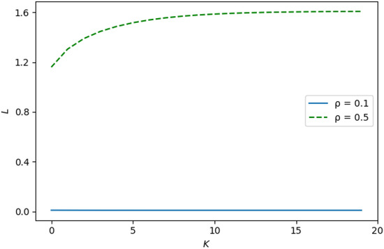
Figure 1. L vs. K for system loads $\rho =0.1$ and $\rho =0.5$.

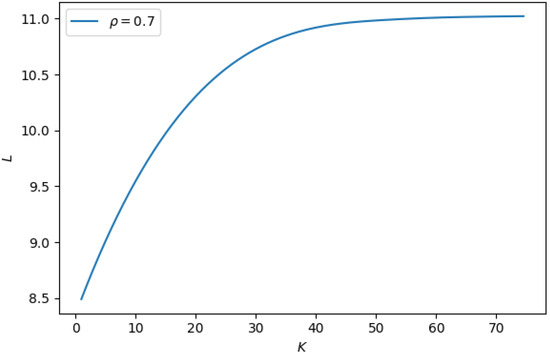
Figure 2. L vs. K for system load $\rho =0.7$.

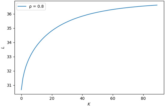
Figure 3. L vs. K for system load $\rho =0.8$.

The following conclusions can be drawn from Table 1 and Figure 1, Figure 2 and Figure 3:

1.

For the system loads $\rho =0.1,0.5,0.7,0.8,$ there are finite values of $K=K_{max}=19,19,76,89,$ respectively, such that with a further increase in this value, the average number of customers in the orbit, L, practically does not change. Here and below, the words “practically does not change” mean that $\frac{L(K_{max}-1)-L\left(K_{max}\right)}{L\left(K_{max}\right)}\ast 100\%<0.04\%.$ The value of $K_{max}$ increases with the system load $\rho$ increasing. However, for all values of $\rho$, the value of $K_{max}$ is not so large that problems with the dimension of the involved matrices appear when calculating the stationary distribution. Thus, it follows from the results of this experiment that the system with such a threshold $K_{max}$ can serve as a good approximation of the retrial $BMAP/PH/N$ queue with the $PH$ distribution of inter-retrial times;

2.

Recall that the value of L for $K=0$ corresponds to the system with exponential inter-retrial times, while the value of L for $K=K_{max}$ corresponds to the system with $PH$ inter-retrial times. As seen from Table 1 and Figure 1, Figure 2 and Figure 3, these values are quite different. If we consider the value of L for $K=0$ as an estimate of the value of L for $K=K_{max}$, then we can see that this estimate is too optimistic, at least for medium and large system loads. Furthermore, the relative errors in calculating L are $27.9\%,24.5\%,14.1\%$ for the values of $\rho =0.5,0,7,0.8,$ respectively. Thus, the retrial $BMAP/PH/N$ queue with exponential inter-retrial times cannot be regarded as a good approximation of the corresponding system with $PH$ inter-retrial times.

Experiment 1.b.

To see how the coefficient of variation of the inter-retrial times affects the value of $K_{max},$ we carried out Experiment 1.b, which was similar to Experiment 1.a, but in which the distribution of inter-retrial times was defined by the vector $\mathit{\tau }=(0.05,0.95)$ and the matrix $T=\left(\begin{array}{cc}-0.88607& 0\\ 0& -70.00013\end{array}\right).$

This means that the inter-retrial time has a hyper-exponential distribution with the rate $\tau =14.28$ and ${\left(c_{var}^{retrial}\right)}^2=25$.

The results of the experiment are displayed in Table 2.

Table 2. The values of L for different values of $\rho$ and K.

K	$\mathit{\rho }=0.1$	$\mathit{\rho }=0.5$	K	$\mathit{\rho }=0.7$	K	$\mathit{\rho }=0.8$
0	0.0085	0.806	0	8.3214	0	31.4536
1	0.0129	1.0521	1	8.4919	1	31.4654
2	0.0167	1.3060	50	14.5908	50	39.8999
3	0.019	1.5016	51	14.5987	51	39.9359
4	0.0201	1.7028	62	14.6518	75	40.4629
5	0.0205	1.8441	63	14.6545	76	40.4759
6	0.0207	2.0066	68	14.6653	87	40.5938
7	0.0207	2.155	69	14.6669	88	40.6026
8	0.0208	2.2867	71	14.6699	93	40.6426
9	0.0208	2.4009	72	14.6712	94	40.65
10	0.0208	2.4978	73	14.6724	96	40.6639
11	0.0208	2.5787	74	14.6735	97	40.6715
12	0.0208	2.6451	75	14.6745	98	40.678
13	0.0208	2.6988
14	0.0208	2.7418
15	0.0208	2.7758
16	0.0208	2.8024
17	0.0208	2.823
18	0.0208	2.8389
19	0.0208	2.8401

First, from Table 2, we can draw the conclusions that were already indicated for the similar Experiment 1.a. Second, comparing the results of the last two experiments, which differed in the value of coefficient of variation (${\left(c_{var}^{retrial}\right)}^2=1.24$ and ${\left(c_{var}^{retrial}\right)}^2=25)$ of inter-retrial times, we can see that coefficient of variation affects the value of L (increases with $c_{var}^{retrial}$ increasing), but does not practically affect the threshold $K_{max}$.

Experiment 2. The purpose of this experiment was to investigate how the performance indicators of the system, L and $P_{imm},$ depend on the rate of retrials for inter-retrial times with different coefficients of variation.

In the experiment, the input data were the same as in Experiment 1, except the distribution of inter-retrial times. Besides, we modified the matrices $D_0$ and D to obtain the arrival rate that provides the system load $\rho =0.5.$

We considered four variants of the $PH$ distribution of inter-retrial times with the same rate $\tau =14.28$, but with different coefficients of variation. To change the rate of retrials, $\tau$, we multiplied the matrix T by the corresponding constants. We calculated the performance indicators of the system fixing $K=30$, since, as we found earlier, such a value of K is suitable in the case $\rho =0.5.$

The first variant is the Erlang distribution of order two with ${\left(c_{var}^{retrial}\right)}^2=0.5$ defined by the following vector and matrices:

$$\mathit{\tau }=(1,0),T=\left(\begin{array}{cc}-28.57& 28.57\\ 0& -28.57\end{array}\right).$$

The second variant is the exponential distribution with $c_{var}^{retrial}=1$ defined by the rate $\mathit{\tau }=14.28.$

The third variant is the hyper-exponential distribution with ${\left(c_{var}^{retrial}\right)}^2=25$ defined by the following vector and matrices:

$$\mathit{\tau }=(0.98,0.02),T=\left(\begin{array}{cc}-142870& 0\\ 0& -0.2857\end{array}\right).$$

The fourth variant is the hyper-exponential distribution with ${\left(c_{var}^{retrial}\right)}^2=98.98$ defined by the following vector and matrices:

$$\mathit{\tau }=(0.05,0.95),T=\left(\begin{array}{cc}-0.88607& 0\\ 0& -70.00013\end{array}\right).$$

In all cases, we considered the threshold $K_{max}=30$. We are sure that such a choice of the threshold is sufficient for all systems considered in this experiment to be a good approximation of the corresponding systems with the $PH$ distribution of inter-retrial times. This assumption was based on the conclusion to Experiment 1.b. According to these points, the value of $K_{max}$ increases with the system load increasing, but the coefficient of variation does not practically affect the threshold $K_{max}$. It follows from Table 1 and Table 2 that for the load $\rho =0.5$, it is sufficient to set $K_{max}=19$ in order to obtain a good approximation of the systems with the $PH$ distribution of inter-retrial times. We took $K_{max}=30$, which, in our opinion, is quite enough to obtain a good approximation.

Figure 4 and Figure 5 depict the behavior of the average number of customers in the orbit, $L,$ and the probability of immediate access to the service, $P_{imm},$ depending on the retrial rate for the $PH$ distributions of inter-retrial times with different coefficients of variation.

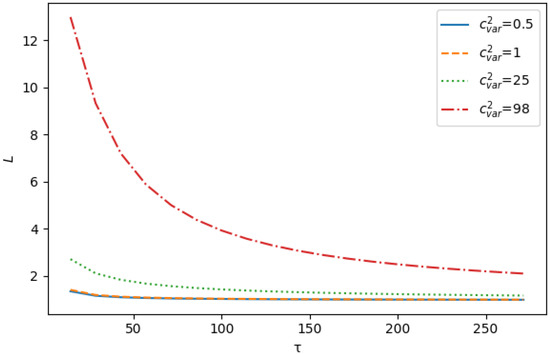
Figure 4. L vs. $\tau$ for the inter-retrial times with different coefficients of variation.

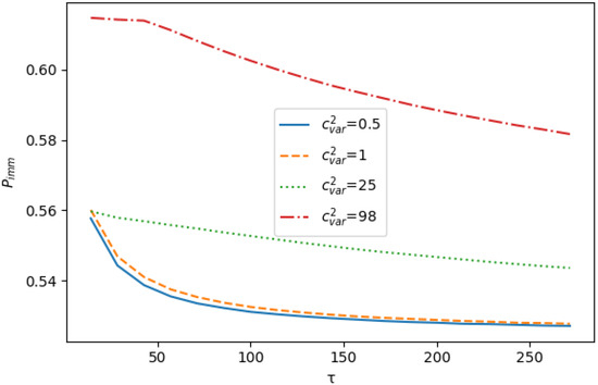
Figure 5. $P_{imm}$ vs. $\tau$ for the inter-retrial times with different coefficients of variation.

Both characteristics under study, as expected, decrease with increasing the parameter $\tau$ (in the pictures $\tau \ge 14.28$) and at large values of $\tau$ their values tend to the values of the corresponding characteristics for the system with an infinite buffer. A more interesting observation is that for fixed $\tau$, both characteristics increase with increasing the inter-retrial time variation. This may be due to the fact that with significant fluctuations in the value of this time, a customer from the orbit may meet a free server less often. This implies that the number of orbital customers increases. At the same time, the increase of the variation can generate the non-uniformity of the process of occupying servers by orbital customers, which implies a greater chance for a primary customer to meet a free server.

Experiment 3. The purpose of this experiment was to find out how the average number of customers in the orbit, L, and the probability of immediate access to the service, $P_{imm},$ depend on the input rate $\lambda$ for the $BMAP$s with different coefficients of correlation.

We considered the following input data: $N=5$; the service time has the Erlang distribution with parameters $(2,10)$; inter-retrial times have hyper-exponential distribution with $\left(c_{var}^{serv}\right)=98.98$ and are defined by the following vector and matrix:

$$\mathit{\tau }=(0.05,0.95),T=\left(\begin{array}{cc}-0.88607& 0\\ 0& -70.00013\end{array}\right).$$

We considered three $BMAP$s with the same arrival rate $\lambda =1.85$, but with different coefficients of correlation. To construct these $BMAP$s, we first define three $MAP$s.

The first $MAP$ is the stationary Poisson process with input rate $\lambda =1.85.$ For this $MAP$, $c_{cor}=0.$

The second $MAP$ is defined by the matrices:

$$D_0=\left(\begin{array}{cc}-1.3526& 0\\ 0& -0.04391\end{array}\right),D=\left(\begin{array}{cc}1.3436& 0.009\\ 0.02446& 0.01945\end{array}\right).$$

For this $MAP$, $c_{cor}=0.2;$

The third $MAP$ is defined by the matrices:

$$D_0=\left(\begin{array}{cc}-3.4& 0\\ 0.00101& -0.1103\end{array}\right),D=\left(\begin{array}{cc}3.3645& 0.0354\\ 0.0121& 0.0971\end{array}\right).$$

For this $MAP$, $c_{cor}=0.4.$

Based on these $MAP$s, we constructed three $BMAP$s. For each of these $BMAP$s, the maximal size of the batch was assumed to be three. This means that the $BMAP$ is defined by the matrices $D_k,k=\overline{0,3}.$ To build these matrices, we followed such a way. The matrix $D_0$ is the same as in the corresponding $MAP$, and the matrices $D_k,k=\overline{1,3},$ are calculated by the formula $D_k=D{q}^{k-1}(1-q)/(1-q^3),k=\overline{1,3},$ where $q=0.8$.

In all cases, we assumed that the threshold $K=30.$

Figure 6 and Figure 7 depict the average number of customers in the orbit, L, and the probability of immediate access to the service, $P_{imm},$ as functions of the input rate $\lambda$ for $BMAP$s with different coefficients of correlation.

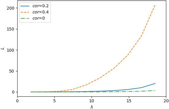
Figure 6. L vs. $\lambda$ for $BMAP$s with different coefficients of correlation.

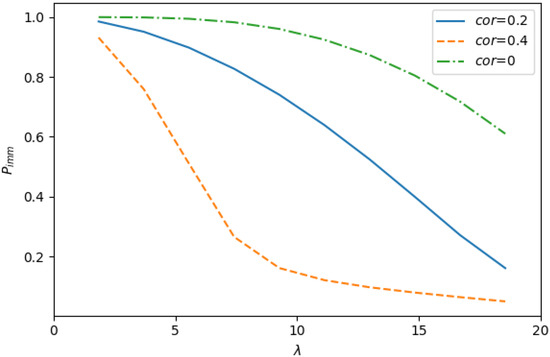
Figure 7. $P_{imm}$ vs. $\lambda$ for $BMAP$s with different coefficients of correlation.

As seen from Figure 6 and Figure 7, under the same value of input rate $\lambda$, the performance indicators under study significantly depend on the correlation in the input flow. With increasing the coefficient of correlation, these indicators become worse: the value of L increases and the value of $P_{imm}$ decreases. From this observation, it can be concluded that when evaluating the performance indicators of the system, it is extremely important to take into account the correlation in the input flow.

7. Conclusions

In this paper, we studied the retrial $BMAP/PH/N$ system with a threshold policy for the inter-retrial time distribution. The novelty of this study was that we took into account the non-exponentiality of the time between retrials in the case when the number of customers in orbit does not exceed the threshold. We assumed that inter-retrial time intervals have the $PH$ distribution if the number of orbital customers is no more than the predetermined threshold and they have an exponential distribution with the same rate otherwise. We described the operation of the system by the asymptotically quasi-Toeplitz Markov chain, derived the constructive stability condition, and calculated the stationary distribution and the main performance indicators of the system. We showed numerically that there exists such a threshold value for which our model is still amenable to numerical computation and at the same time can serve as a good approximation of the $BMAP/PH/N$ system with the $PH$ distribution of inter-retrial times. Having found such a threshold value, we further calculated the performance indicators and considered them to be the performance indicators of the $BMAP/PH/N$ queueing system with the $PH$ distribution of inter-retrial times. We compared numerically our threshold queueing model with the corresponding queueing model having exponentially distributed inter-retrial times. We also presented a number of illustrative numerical examples to analyze the behavior of the system performance indicators depending on the system parameters, the variance of the inter-retrial times, and the correlation in the input flow. Mathematically, the considered system is more general than analogs known in the literature and is of independent interest as a fairly adequate model of information exchange processes in modern telecommunication networks.

References

- Artalejo, J. Accessible bibliography on retrial queues. Math. Comput. Model. 1999, 30, 223–233. [Google Scholar] [CrossRef]
- Gomez-Corral, A. A bibliographical guide to the analysis of retrial queues through matrix analytic techniques. Ann. Oper. 2006, 141, 163–191. [Google Scholar] [CrossRef]
- Falin, G.; Templeton, J. Retrial Queues; Chapman and Hall: London, UK, 1997. [Google Scholar]
- Artalejo, J.R.; Gomez-Corral, A. Retrial Queueing Systems: A Computational Approach; Springer: Berlin/Heidelberg, Germany, 2008. [Google Scholar]
- Lucantoni, D. New results on the single server queue with a batch Markovian arrival process. Commun. Statist.-Stoch. Models 1991, 7, 1–46. [Google Scholar] [CrossRef]
- Choi, B.D.; Shin, Y.W.; Ahn, W.C. Retrial queues with collision arising from unslottted CDMA/CD protocol. Queueing Syst. 1992, 11, 335–356. [Google Scholar] [CrossRef]
- Gomez-Corral, A. Stochastic analysis of a single server retrial queue with general retrial time. Nav. Res. Logist. 1999, 46, 561–581. [Google Scholar] [CrossRef]
- Moreno, P. An M/G/1 retrial queue with recurrent customers and general retrial times. Appl. Math. Comput. 2004, 159, 651–666. [Google Scholar] [CrossRef]
- Atencia, I.; Moreno, P. A single server retrial queue with general retrial time and Bernoulli schedule. Appl. Math. Comput. 2005, 162, 855–880. [Google Scholar] [CrossRef]
- Choudhury, G. An M/G/1 retrial queue with an additional phase of second service and general retrial time. Int. J. Inf. Manag. Sci. 2009, 20, 1–14. [Google Scholar]
- Krishna Kumar, B.; Vijay Kumar, A.; Arivudainambi, D. An M/G/1 retrial queueing system with two phase service and preemptive resume. Ann. Oper. Res. 2002, 113, 61–79. [Google Scholar] [CrossRef]
- Wu, X.; Brill, P.; Hlynka, M.; Wang, J. An M/G/1 retrial queue with balking and retrials during service. Int. J. Oper. Res. 2005, 1, 30–51. [Google Scholar] [CrossRef]
- Choudhury, G.; Ke, J.C. A batch arrival retrial queue with general retrial times under Bernoulli vacation schedule for unreliable server and delaying repair. Appl. Math. Model. 2012, 36, 255–269. [Google Scholar] [CrossRef]
- Yang, T.; Posner, M.J.M.; Templeton, J.G.C.; Li, H. An approximation method for the M/G/1 retrial queue with general retrial times. Eur. J. Oper. Res. 1994, 76, 110–116. [Google Scholar] [CrossRef]
- Liang, H.M. Retrial Queues (Queueing System, Stability Condition, K-Ordering). Ph.D. Thesis, University of North Carolina, Chapel Hill, NC, USA, 1991. [Google Scholar]
- Diamond, J.E.; Alfa, A.S. An approximation method for the M/PH/1 retrial queue with phase-type inter-retrial times. Eur. J. Oper. Res. 1999, 113, 620–631. [Google Scholar] [CrossRef]
- Shin, Y.W. Algorithmic solutions for M/M/c retrial queue with PH2 retrial time. J. Appl. Math. Inform. 2011, 29, 803–811. [Google Scholar]
- Shin, Y.W.; Moon, D.H. Approximation of M/M/c retrial queue with PH-retrial times. Eur. J. Oper. Res. 2011, 213, 205–209. [Google Scholar] [CrossRef]
- Chakravarthy, S.R. A retrial ququeing model with thresholds and phase-type retrial times. J. Appl. Math. Inform. 2020, 38, 351–373. [Google Scholar] [CrossRef]
- Chakravarthy, S.R.; Ozkar, S.; Shruti, S. Analysis of M/M/c Retrial Queue with Thresholds, PH Distribution of Retrial Times and Unreliable Servers. J. Appl. Math. Inform. 2021, 39, 173–196. [Google Scholar] [CrossRef]
- Dudin, A.; Shaban, A.; Klimenok, V. Analysis of a queue in the BMAP/G/1/N system. Int. J. Simul. Syst. Sci. Technol. 2005, 6, 13–23. [Google Scholar]
- Breuer, L.; Dudin, A.; Klimenok, V. A retrial BMAP/PH/N system. Queueing Syst. 2002, 40, 433–457. [Google Scholar] [CrossRef]
- Klimenok, V.; Orlovsky, D.; Dudin, A. A BMAP/PH/N system with impatient repeated calls. Asia-Pac. J. Oper. Res. 2007, 24, 293–312. [Google Scholar] [CrossRef]
- Breuer, L.; Klimenok, V.; Birukov, A.; Dudin, A.; Krieger, U. Mobile networks modeling the access to a wireless network at hot spots. Eur. Trans. Telecommun. 2005, 16, 309–316. [Google Scholar] [CrossRef]
- Kim, C.S.; Klimenok, V.; Mushko, V.; Dudin, A. The BMAP/PH/N retrial queueing system operating in Markovian random environment. Comput. Oper. Res. 2010, 37, 1228–1237. [Google Scholar] [CrossRef]
- Klimenok, V.I.; Orlovsky, D.S.; Kim, C.S. The BMAP/PH/N retrial queue with Markovian flow of breakdowns. Eur. J. Oper. Res. 2008, 189, 1057–1072. [Google Scholar]
- Kim, C.S.; Park, S.H.; Dudin, A.; Klimenok, V.; Tsarenkov, G. Investigaton of the BMAP/G/1→./PH/1/M tandem queue with retrials and losses. Appl. Math. Model. 2010, 34, 2926–2940. [Google Scholar] [CrossRef]
- Dayar, T.; Orhan, V.C. Steady-state analysis of a multiclass MAP/PH/c queue with acyclic PH retrials. J. Appl. Prob. 2016, 53, 1098–1110. [Google Scholar] [CrossRef]
- Chakravarthy, S.R. Analysis of MAP/PH/c retrial queue with phase-type retrials—Simulation approach. Commun. Comput. Inf. Sci. 2013, 356, 37–49. [Google Scholar]
- Ramaswami, V. Independent Markov processes in parallel. Commun. Statist.-Stoch. Models 1985, 1, 419–432. [Google Scholar] [CrossRef]
- Ramaswami, V.; Lucantoni, D. Algorithms for the multi-server queue with phase-type service. Commun. Statist.-Stoch. Models 1985, 1, 393–417. [Google Scholar] [CrossRef]
- Klimenok, V.; Dudin, A.; Vishnevsky, V. A Retrial Queueing System with Alternating Inter-Retrial Time Distribution. Commun. Comput. Inf. Sci. 2018, 919, 302–315. [Google Scholar]
- Neuts, M.F. Structured Stochastic Matrices of M/G/1 Type and Their Applications; Marcel Dekker: New York, NY, USA, 1989. [Google Scholar]
- Graham, A. Kronecker Product and Matrix Calculus with Applications; Ellis Horwood Ltd.: Chichester, UK, 1981. [Google Scholar]
- Kim, C.S.; Mushko, V.V.; Dudin, A. Computation of the steady state distribution for multi-server retrial queues with phase-type service process. Ann. Oper. Res. 2012, 201, 307–323. [Google Scholar] [CrossRef]
- Kim, C.S.; Dudin, S.; Taramin, O.; Baek, J. Queueing system MMAP/PH/N/N+R with impatient heterogeneous customers as a model of call center. Appl. Math. Model. 2013, 37, 958–976. [Google Scholar] [CrossRef]
- Dudin, A.N.; Klimenok, V.I.; Vishnevsky, V.M. The Theory of Queuing Systems with Correlated Flows; Springer: Cham, Switzerland, 2019. [Google Scholar]
- Klimenok, V.I.; Dudin, A.N. Multi-dimensional asymptotically quasi-Toeplitz Markov chains and their application in queueing theory. Queueing Syst. 2006, 54, 245–259. [Google Scholar] [CrossRef]
Publisher’s Note: MDPI stays neutral with regard to jurisdictional claims in published maps and institutional affiliations. |
© 2022 by the authors. Licensee MDPI, Basel, Switzerland. This article is an open access article distributed under the terms and conditions of the Creative Commons Attribution (CC BY) license (https://creativecommons.org/licenses/by/4.0/).