A Non-Iterative Method for the Difference of Means on the Lie Group of Symmetric Positive-Definite Matrices

Abstract

A non-iterative method for the difference of means is presented to calculate the log-Euclidean distance between a symmetric positive-definite matrix and the mean matrix on the Lie group of symmetric positive-definite matrices. Although affine-invariant Riemannian metrics have a perfect theoretical framework and avoid the drawbacks of the Euclidean inner product, their complex formulas also lead to sophisticated and time-consuming algorithms. To make up for this limitation, log-Euclidean metrics with simpler formulas and faster calculations are employed in this manuscript. Our new approach is to transform a symmetric positive-definite matrix into a symmetric matrix via logarithmic maps, and then to transform the results back to the Lie group through exponential maps. Moreover, the present method does not need to compute the mean matrix and retains the usual Euclidean operations in the domain of matrix logarithms. In addition, for some randomly generated positive-definite matrices, the method is compared using experiments with that induced by the classical affine-invariant Riemannian metric. Finally, our proposed method is applied to denoise the point clouds with high density noise via the K-means clustering algorithm.

1. Introduction

The difference of means method is usually employed in detection problems. Its procedure can be described as Figure 1: for the detected element $R_0$, the distance between $R_0$ and the mean of the reference elements $R_{-N},\dots ,R_{-1}$, $R_1,\dots ,R_N$ is computed. If the distance is bigger than the present value, we can conclude that $R_0$ can be distinguished from the reference elements. For example, the difference of means method is applied to detect abnormal conditions in clustered enterprise middleware systems [1,2,3]. In [4], an algorithm is proposed to detect the change-points of rigid body motions, which is defined as the difference of means method in the special Euclidean group. Based on the difference of means method, a geometric approach is developed for high-resolution Doppler processing and shows the existence of targets in fixed directions of some elements [5].

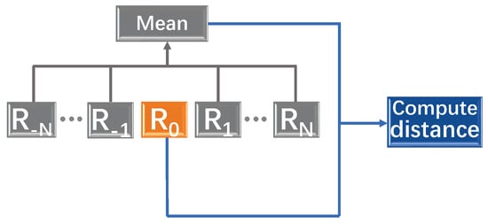
Figure 1. The difference of means method.

In the field of coastal radars, the issue of detecting small targets and stealth targets in a non-uniform clutter environment is vital. Recently, a high-resolution Doppler detector was proposed by Ref. [6] using the difference of means method, and the X-band radar experiments at Paris Airport show that the performance of Doppler imaging and Doppler detection has been improved. Their purpose of target detection is to judge whether there are targets in some cells according to the observed values. Based on the affine-invariant Riemannian metric, they developed an iterative algorithm for the Riemannian mean of some symmetric positive-definite Hermitian matrices.

In this paper, we propose a non-iterative method to compute the distance between a symmetric positive-definite matrix and the mean matrix on the Lie group of symmetric positive-definite matrices. Although affine-invariant Riemannian metrics, which avoid the drawbacks of Euclidean inner product, have a perfect theoretical framework, their complex formulas also lead to sophisticated and time-consuming algorithms [7,8]. Therefore, we use log-Euclidean metrics to obtain simpler formulas and faster calculations [9,10,11]. As the Lie algebra of the Lie group is the space of symmetric matrices, we transform the Riemannian computations on the Lie group into Euclidean computations on its Lie algebra. Finally, our proposed method is applied to denoise the point clouds with high density noise via the K-means clustering algorithm.

Our first contribution is that a non-iterative method for calculating the log-Euclidean distance between a symmetric positive-definite matrix and the mean matrix is obtained, and the mean matrix does not need to be calculated. Our second contribution is applied our proposed method to denoise the point clouds with high density noise via the K-means clustering algorithm, and the denoising effect of the method is evaluated by three criteria: Accuracy, Recall and Precision.

The remaining sections of this paper are as follows: Section 2 reviews the geometry on the space of symmetric positive-definite matrices, including metrics, geodesics and geodesic distances. In Section 3, a non-iterative method is presented to compute the distance between a matrix and the mean matrix on the Lie group of symmetric positive-definite matrices, and the method is compared with classical algorithms using simulations. Section 4 shows the effectiveness of our developed method to denoise the point clouds with high density noise.

2. Preliminaries

In this section, we introduce some concepts, including Euclidean metrics, affine-invariant Riemannian metrics and log-Euclidean metrics on the space of symmetric positive-definite matrices. More details are discussed in Refs. [12,13,14,15].

2.1. Exponential Map and Logarithmic Map

The set of all invertible $n\times n$ real matrices is known as the general linear group $\mathrm{GL}(n,\mathbb{R})$. The set of all $n\times n$ real matrices is denoted by $M_{n\times n}$, where $\mathrm{GL}(n,\mathbb{R})$ is a differentiable manifold and $M_{n\times n}$ is the Lie algebra $\mathfrak{gl}(n,\mathbb{R})$. Exponential maps and logarithmic maps can transmit the information between $\mathrm{GL}(n,\mathbb{R})$ and $M_{n\times n}$. Here, the exponential map of a matrix $V\in M_{n\times n}$ is $M_{n\times n}\to \mathrm{GL}(n,\mathbb{R})$ and expressed by the convergent series

$$exp\left(V\right)=\sum _{k=0}^{\infty }\frac{V^k}{k!}.$$

(1)

On the other hand, the logarithmic map is the local inverse of the exponential map, denoted by log and the logarithmic map of a matrix $A\in \mathrm{GL}(n,\mathbb{R})$ is the solution of the equation $expV=A$. When all eigenvalues of A are non-negative, there exists a unique real logarithm, whose spectrum is just in the scope $\{z\in \mathbb{C}:-\pi <\mathrm{Im}(z)<\pi \}$ of the complex plane [16]. Furthermore, if A is in a neighborhood of the identity matrix I, then the series ${\sum }_{k=1}^{\infty }{(-1)}^{k+1}\frac{{(A-I)}^k}{k}$ converges to $logA$. The logarithmic map is shown in

$$log\left(A\right)=\sum _{k=1}^{\infty }{(-1)}^{k+1}\frac{{(A-I)}^k}{k}.$$

(2)

Let us denote the set of all the $n\times n$ symmetric matrices by

$$S\left(n\right)=\{V\in M_{n\times n}|V^T=V\}$$

(3)

and the set of all the $n\times n$ symmetric positive-definite matrices by

$$\mathrm{P}\left(n\right)=\{A\in S(n\left)\right|A>0\},$$

(4)

where $A>0$ implies that the quadratic form $x^{T}Ax>0$ for all non-zero n-dimensional vectors x. For a general invertible matrix, the uniqueness and existence of logarithmic maps may not be available. The logarithm of a symmetric positive-definite matrix is well defined and is a symmetric matrix. Moreover, since the exponential map from $S\left(n\right)$ to $\mathrm{P}\left(n\right)$ is one-to-one and onto, the exponential map of any symmetric matrix is symmetric positive-definite.

2.2. Frobenius Inner Product

On $\mathrm{P}\left(n\right)$, the Frobenius inner product is

$${⟨A,B⟩}_F=\mathrm{tr}\left(A^{T}B\right),$$

(5)

where $\mathrm{tr}(·)$ is the trace of $“·”$, hence $\mathrm{P}\left(n\right)$ with the metric (5) is taken as a manifold. The tangent space at the point $A\in \mathrm{P}\left(n\right)$ is written as $T_A\mathrm{P}\left(n\right)$. Since $\mathrm{P}\left(n\right)$ is an open subset of $S\left(n\right)$, the tangent space $T_A\mathrm{P}\left(n\right)$ at A can be identified with $S\left(n\right)$. The geodesic at A in the direction of $V\in S\left(n\right)$ with the metric (5) is a straight line

$${\gamma }_F\left(t\right)=W+tY,0\le t<\delta ,$$

(6)

with $\delta >0$, where t is sufficiently small so that the geodesic (6) remains on $\mathrm{P}\left(n\right)$. The associated norm ${\parallel A\parallel }_F={⟨A,A⟩}_F^{\frac{1}{2}}$ defines the Euclidean distance on $\mathrm{P}\left(n\right)$ as follows

$$d_F(A,B)={\parallel A-B\parallel }_F.$$

(7)

2.3. Affine-Invariant Riemannian Metric

The Riemannian metric at point A is defined by

$$g_A(V_1,V_2)=g_I(A^{-1}{V}_1,A^{-1}{V}_2)=\mathrm{tr}\left(A^{-1}{V}_1{A}^{-1}{V}_2\right)$$

(8)

with $V_1,V_2\in T_A\mathrm{P}\left(n\right)$, where $\mathrm{P}\left(n\right)$ with the metric (8) is a Riemannian manifold.

At point $A\in \mathrm{P}\left(n\right)$, the geodesic in the direction $V\in T_A\mathrm{P}\left(n\right)$ is given by

$${\gamma }_{Aff}\left(t\right)=A^{\frac{1}{2}}exp\left(t{A}^{-\frac{1}{2}}V{A}^{-\frac{1}{2}}\right)A^{\frac{1}{2}},$$

(9)

which is entirely contained on $\mathrm{P}\left(n\right)$. It is noted that $\mathrm{P}\left(n\right)$ with the metric (8) is geodesically complete [17], then a geodesic curve ${\gamma }_{Aff}\left(t\right)$ can be obtained for any given matrices $A,B\in \mathrm{P}\left(n\right)$, which satisfies that ${\gamma }_{Aff}\left(0\right)=A$, ${\gamma }_{Aff}\left(1\right)=B$ and the initial velocity ${\dot{\gamma }}_{Aff}\left(0\right)=A^{\frac{1}{2}}log\left(A^{-\frac{1}{2}}B{A}^{-\frac{1}{2}}\right)A^{\frac{1}{2}}\in T_A\mathrm{P}\left(n\right)$. The Riemannian distance between A and B is represented as

$$d_{Aff}(A,B)={\parallel log\left(A^{-\frac{1}{2}}B{A}^{-\frac{1}{2}}\right)\parallel }_F.$$

(10)

The following action $act\left(U\right)$ of a matrix $U\in \mathrm{GL}(n,\mathbb{R})$ is defined by

$$act\left(U\right)A=UA{U}^T,\forall A\in \mathrm{P}\left(n\right).$$

(11)

This group action describes the influence of the general affine change of coordinates on the matrix $A\in \mathrm{P}\left(n\right)$. In addition, this action is naturally extended to tangent vectors in the same way. For example, if $\iota \left(t\right)=A+tV+O\left(t^2\right)$ is a curve passing through A with tangent vector V, then the curve $act\left(U\right)\iota \left(t\right)=UA{U}^T+tUV{U}^T+O\left(t^2\right)$ passes through $act\left(U\right)A$ with tangent vector $act\left(U\right)V$. Moreover, $act\left(U\right):\mathrm{P}\left(n\right)\to \mathrm{P}\left(n\right)$ is isometric for any invertible matrix U, namely

$$d_{Aff}(A,B)=d_{Aff}(act\left(U\right)A,act\left(U\right)B),$$

(12)

so the Riemannian metric (8) is affine-invariant.

2.4. Log-Euclidean Riemannian Metric

Here, $\mathrm{P}\left(n\right)$ becomes a Lie group by defining a logarithmic multiplication ⊙ as follows

$$A\odot B:=exp(logA+logB).$$

(13)

The log-Euclidean metric between tangent vectors $V_1$ and $V_2$ at the point $A\in \mathrm{P}\left(n\right)$ is given by

$$g_A(V_1,V_2)=g_I(D_{A}log{V}_1,D_{A}log{V}_2),$$

(14)

where $D_A$ denotes the differential map at the point A. Then, the geodesic ${\gamma }_{LE}\left(t\right)$ between A and B is given by

$${\gamma }_{LE}\left(t\right)=exp((1-t)logA+tlogB),0\le t\le 1,$$

(15)

and it can see that ${\gamma }_{LE}\left(t\right)$ is a straight line in the domain of matrix logarithms. From (14), the log-Euclidean distance between A and B is written as

$$d_{LE}(A,B)={\parallel logA-logB\parallel }_F.$$

(16)

It is evident that the Formula (16) corresponds to the Euclidean distance in the logarithmic domain. From the above formulas, we can see that the framework of the log-Euclidean metric is simpler than that of the affine-invariant metric (8).

Moreover, the log-Euclidean metrics satisfy the following invariance property

$$d_{LE}(A^{-1},B^{-1})=d_{LE}(A,B),$$

(17)

with $A,B\in \mathrm{P}\left(n\right)$. Although the log-Euclidean metrics do not entirely satisfy affine-invariant conditions, they are similarity invariant by an orthogonal transformation

$$d_{LE}(\mathrm{act}\left(a\tilde{U}\right)A,\mathrm{act}\left(a\tilde{U}\right)B)=d_{LE}(A,B),$$

(18)

where $\tilde{U}$ is an orthogonal matrix and $a>0$ is a scaling factor.

3. Non-Iterative Method for the Difference of Means on $\mathbf{P}\left(\mathit{n}\right)$

In this section, for $2N+1$ given matrices on $\mathrm{P}\left(n\right)$, we present a non-iterative method to calculate the distance between a matrix and the mean of the remaining $2N$ matrices. As an introduction, we first review the concept of the mean matrix associated with different metrics.

3.1. Mean Matrices Associated with Different Metrics

For a given metric, the associated mean of m matrices $A_1,\dots ,A_m$ on $\mathrm{P}\left(n\right)$ is defined as the matrix $\mathbb{M}(A_1,\dots ,A_m)$ minimizing the cost function

$$\mathbb{M}(A_1,\dots ,A_m)=\arg min\sum _{i=1}^m{d}^2(A,A_i),$$

(19)

where $d(·,·)$ corresponds to the metric.

First, the mean matrix induced by the Frobenius inner product (5) is represented as

$${\mathbb{M}}_F(A_1,\dots ,A_m)=\frac{1}{m}\sum _{i=1}^m{A}_i,$$

(20)

which is the usual arithmetic mean. Via the convexity of $\mathrm{P}\left(n\right)$, the Frobenius inner product can still be used, but utilizing $\mathrm{P}\left(n\right)$ with this flat metric dose not result in a geodesically complete space. Because of this, it may not be appropriate to adopt the arithmetic mean on this manifold (see Ref. [6]).

The Riemannian mean associated with the affine-invariant metric (8) is not explicit, as denoted by ${\mathbb{M}}_{Aff}\left(A_i\right)$. It can only be computed by the following iterative algorithm [6]

$$A^{(k+1)}={\left(A^{\left(k\right)}\right)}^{\frac{1}{2}}exp(-\eta \sum _{i=1}^{m}log\left({\left(A^{\left(k\right)}\right)}^{-\frac{1}{2}}{A}_i{\left(A^{\left(k\right)}\right)}^{-\frac{1}{2}}\right)){\left(A^{\left(k\right)}\right)}^{\frac{1}{2}},$$

(21)

where $A^{\left(k\right)}$ means the k-th iteration of ${\mathbb{M}}_{Aff}\left(A_i\right)$ and $\eta$ is the learning rate.

Next, the Riemannian mean in the log-Euclidean case is given. The following lemmas are useful for calculating the Riemannian mean [12,18].

Lemma 1.

Let $X,Y$ denote function-valued matrices and A be a constant matrix. We have

$$\mathrm{d}A=0,$$

(22)

$$\mathrm{d}(X\pm Y)=\mathrm{d}X\pm \mathrm{d}Y,$$

(23)

$$\mathrm{d}\left(XY\right)=\left(\mathrm{d}X\right)Y+X\left(\mathrm{d}Y\right),$$

(24)

$$\mathrm{d}\mathrm{tr}\left(X\right)=\mathrm{tr}\left(\mathrm{d}X\right).$$

(25)

Moreover, if the matrix X is invertible and all its eigenvalues are positive, then

$$\mathrm{tr}(\mathrm{d}logX)=\mathrm{tr}\left(X^{-1}\mathrm{d}X\right),$$

(26)

$$\mathrm{tr}\left(\mathrm{d}{log}^{2}X\right)=2\mathrm{tr}(logX{X}^{-1}\mathrm{d}X).$$

(27)

Lemma 2.

Let $F\left(X\right)$ denote a scalar function of $n\times n$ matrix X. We have the following properties

$$\mathrm{d}F\left(X\right)=\mathrm{tr}\left(W\mathrm{d}X\right)$$

(28)

is equivalent to

$$\frac{\partial F\left(X\right)}{\partial X}=W^T,$$

(29)

where $\frac{\partial F\left(X\right)}{\partial X}$ stands for the gradient of $F\left(X\right)$ at X.

By the above lemmas, we get the Riemannian mean with the log-Euclidean metric as follows.

Lemma 3.

For m given matrices $A_i$ on $P\left(n\right)$, the Riemannian mean with the associated log-Euclidean metric (14) is obtained by

$${\mathbb{M}}_{LE}(A_1,\dots ,A_m)=exp(\frac{1}{m}\sum _{i=1}^{m}log{A}_i).$$

(30)

Proof. 

According to (16) and (19), the Riemannian mean of $A_1,\dots ,A_m$ minimizes the following cost function

$$J\left(A\right)=\sum _{i=1}^m{\parallel logA-log{A}_i\parallel }_F^2=\sum _{i=1}^m\mathrm{tr}{(logA-log{A}_i)}^2.$$

(31)

Using Lemma 1, the differential of the cost function $J\left(A\right)$ at A is

$$\begin{array}{ccc}\hfill dJ\left(A\right)& =& 2{\sum }_{i=1}^m\mathrm{tr}\left((logA-log{A}_i)A^{-1}dA\right)\hfill \\ \hfill & =& 2\mathrm{tr}\left((mlogA-{\sum }_{i=1}^{m}log{A}_i)A^{-1}dA\right).\hfill \end{array}$$

(32)

By means of Lemma 2 and the symmetry of matrices on $\mathrm{P}\left(n\right)$, we can obtain the gradient of $J\left(A\right)$ at A as

$$\frac{\partial J\left(A\right)}{\partial A}=A^{-1}(mlogA-\sum _{i=1}^{m}log{A}_i).$$

(33)

The necessary condition and sufficient condition for A to be the minimum of $J\left(A\right)$ is

$$\frac{\partial J\left(A\right)}{\partial A}=A^{-1}(mlogA-\sum _{i=1}^{m}log{A}_i)=0,$$

(34)

and the explicit expression of A is given by

$$A=exp(\frac{1}{m}\sum _{i=1}^{m}log{A}_i).$$

(35)

With this, the proof is completed.   □

It can be seen that the log-Euclidean mean (30) is simpler than the affine-invariant one with the iterative Formula (21), and Lemma 3 is Euclidean in the logarithmic domain.

3.2. Non-Iterative Method for the Difference

With the above work, a non-iterative method is proposed to calculate the Riemannian distance between a matrix and the mean of some matrices.

For $2N+1$ given $R_{-N},\dots ,R_{-1},R_0,R_1,\dots ,R_N$ on $\mathrm{P}\left(n\right)$, $R_0$ plays the role of being detected matrices in the algorithms proposed by Refs. [1,5,6].

Since the affine-invariant Riemannian framework with the iterative Formula (21) contains matrix exponential, logarithm, square root and inverse operations, it is time-consuming in practical applications. Although several other scholars have also proposed gradient descent algorithms for the Riemannian mean [6,19,20], all these algorithms are iterative. Therefore, the log-Euclidean Riemannian framework is adopted in our method so that computations on the Lie group $\mathrm{P}\left(n\right)$ being a Riemannian manifold is transformed to calculations on $S\left(n\right)$ being a Euclidean space in the domain of matrix logarithms.

Initially, we transform all the matrices into symmetric matrices by the matrix logarithm

$$log{R}_i:=X_i,$$

(36)

where $-N\le i\le N$. Then, let $X_{i+1}-X_i:={\tau }_i$ and

$$\sum _{k=0}^{N-1}\frac{N-k}{2N}{\tau }_k:=Right\left(X_0\right),\sum _{k=0}^{N-1}\frac{k+1}{2N}{\tau }_{k-N}:=Left\left(X_0\right).$$

(37)

$Right\left(X_0\right)$ stands for the right weighted mean of $X_1,X_2,\dots ,X_N$ after $X_0$ and $Left\left(X_0\right)$ stands for the left weighted mean of $X_{-N},\dots ,X_{-1}$ before $X_0$. Therefore, we can represent the log-Euclidean distance between $R_0$ and ${\mathbb{M}}_{LE}(R_i\backslash R_0)$ by the following theorem, where $R_i\backslash R_0$ stands for $R_{-N},\dots ,R_{-1},R_1,\dots ,R_N$.

Theorem 1.

For $2N+1$ given $R_{-N},\dots ,R_{-1},R_0,R_1,\dots ,R_N$ on $P\left(n\right)$, the log-Euclidean distance between $R_0$ and the mean of the remain $2N$ matrices $R_{-N},\dots ,R_{-1},R_1,\dots ,R_N$ is obtained by

$$d_{LE}(R_0,{\mathbb{M}}_{LE}(R_i\backslash R_0))={\parallel Right\left(X_0\right)-Left\left(X_0\right)\parallel }_F.$$

(38)

Proof. 

From Lemma 3 and (17), the log-Euclidean distance between $R_0$ and the mean of the remain ing $2N$ matrices $R_{-N},\dots ,R_{-1},R_1,\dots ,R_N$ is given by

$$d_{LE}(R_0,{\mathbb{M}}_{LE}(R_i\backslash R_0))={\parallel \frac{1}{2N}\sum _{k=1}^N(log{R}_{-k}+log{R}_k)-log{R}_0\parallel }_F.$$

(39)

We can rewrite the Formula (39) as follows

$$\begin{array}{ccc}{d}_{LE}(R_0,{\mathbb{M}}_{LE}(R_i\backslash R_0))& =& \parallel \frac{1}{2N}{\sum }_{k=1}^N(X_{-k}+X_k)-X_0{\parallel }_F\hfill \\ & =& \parallel {\sum }_{k=0}^{N-1}\frac{N-k}{2N}{\tau }_k-{\sum }_{k=0}^{N-1}\frac{k+1}{2N}{\tau }_{k-N}{\parallel }_F.\hfill \end{array}$$

(40)

This means that $d_{LE}(R_0,{\mathbb{M}}_{LE}(R_i\backslash R_0))$ can be expressed by the difference of the right mean $Right\left(X_0\right)$ and the left mean $Left\left(X_0\right)$.

This completes the proof of Theorem 1.  □

Obviously, the Formula (38) for calculating the log-Euclidean distance between $R_0$ and the mean of the remain $2N$ matrices $R_{-N},\dots ,R_{-1},R_1,\dots ,R_N$ is non-iterative, and the Riemannian mean ${\mathbb{M}}_{LE}(R_i\backslash R_0))$ does not need to be computed. $\mathrm{P}\left(n\right)$ with the log-Euclidean metric (14) is isomorphic and isometric with the corresponding Euclidean $S\left(n\right)$ [15], therefore the calculation in the Log-Euclidean framework should be time-efficient.

3.3. Numerical Examples

Three examples are provided in the present subsection. One illustrates the difference of the arithmetic mean, the affine-invariant mean and the log-Euclidean mean on $\mathrm{P}\left(n\right)$. Two other examples demonstrate the numerical behavior of our proposed method for the calculation of $d_{LE}(R_0,{\mathbb{M}}_{LE}(R_i\backslash R_0))$ and compares the performance with the algorithm proposed by Ref. [6].

In the following simulations, the error criterion of the iterative Formula (21) is

$$d_{Aff}(A^{(k+1)},A^k)<{10}^{-15},$$

(41)

and all samples on $\mathrm{P}\left(n\right)$ are generated by the rule

$$exp\left(\frac{V+V^T}{2}\right),$$

(42)

where $V\in {\mathbb{R}}^{n\times n}$ is a random matrix so that $\frac{V+V^T}{2}\in S\left(n\right)$.

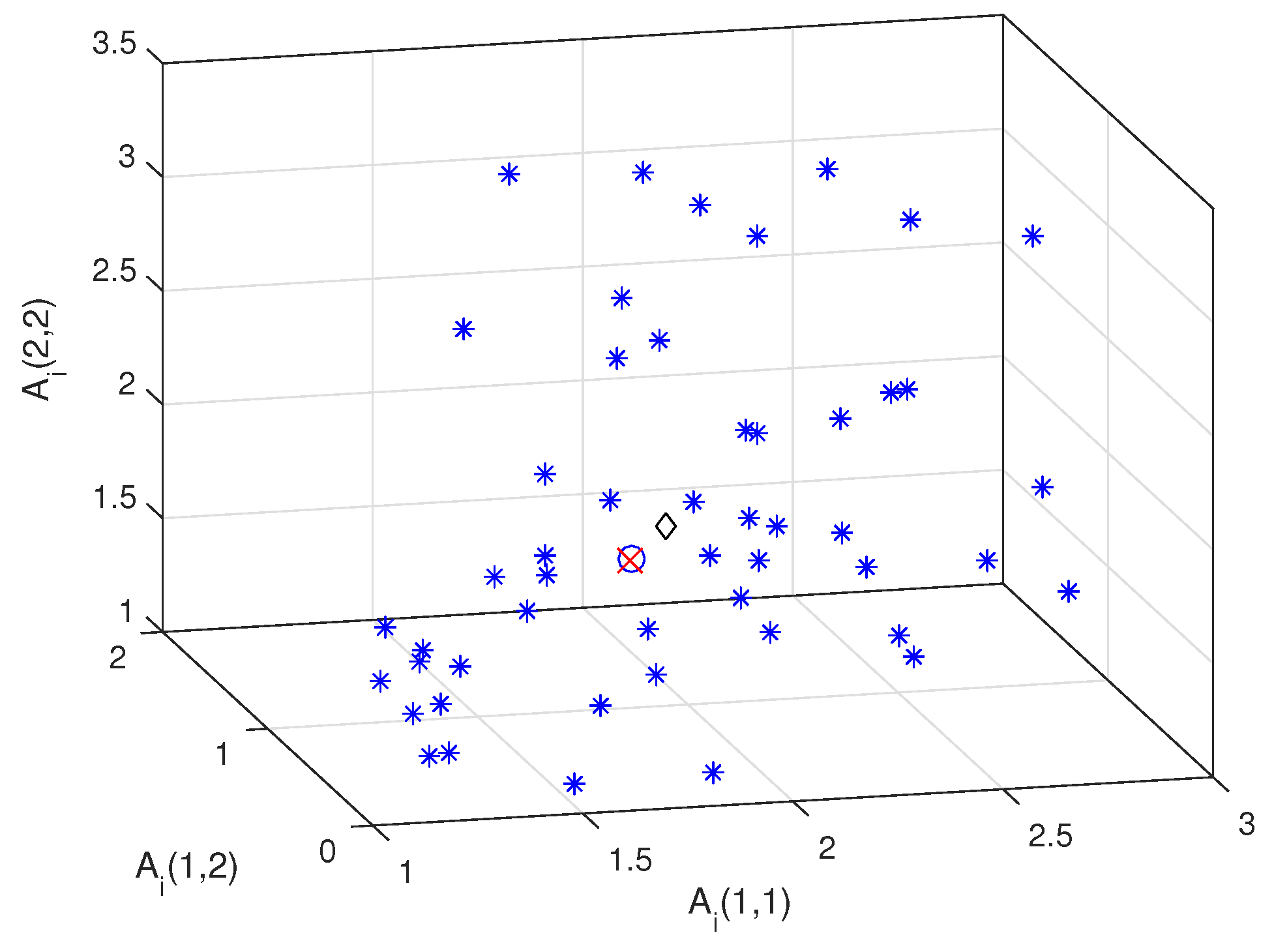
Example 1.

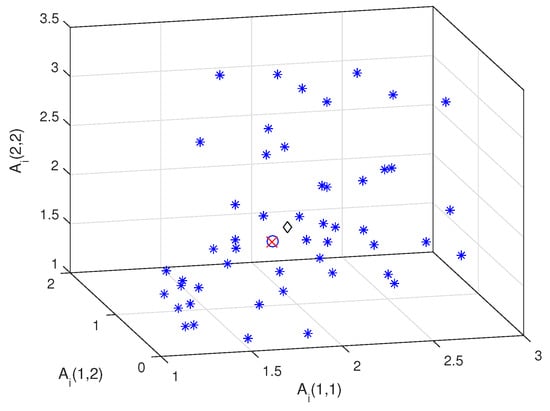
First, we consider a 3-dimensional manifold $P\left(2\right)$ to display symmetric positive-definite matrices in the XYZ system. Figure 2 shows the arithmetic mean (diamond), the affine-invariant mean (circle) and the log-Euclidean mean (cross) of 50 randomly generated matrices (asterisk). It can be seen that the locations of the log-Euclidean mean are very close to that of the affine-invariant mean.

Figure 2. Mean of 50 samples.

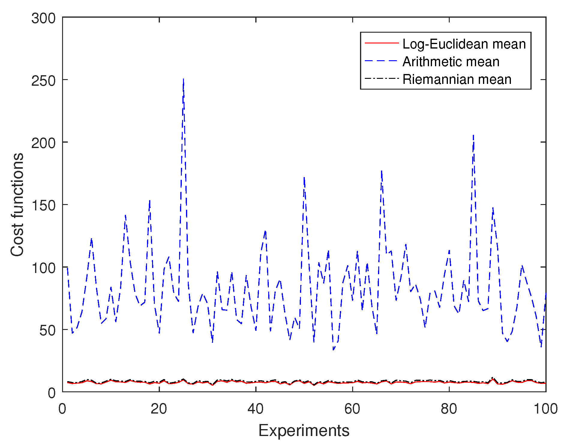
Then, for 10 randomly generated samples $A_1,\dots ,A_{10}$ on $\mathrm{P}\left(4\right)$, we use 50 experiments to compare the cost functions ${\sum }_{i=1}^{10}{d}^2(A,A_i)$ of the arithmetic mean, the affine-invariant mean and the log-Euclidean mean. Figure 3 shows that the cost function of the log-Euclidean mean is the smallest of them, and that the cost function of the arithmetic mean is much larger than the others. It can be seen that the cost function of the log-Euclidean mean is very close to that of the Riemannian mean, and the difference between them is less than 1.3 for this set of experimental data.

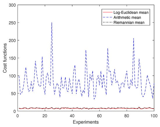
Figure 3. Comparison of cost functions.

Therefore, it is shown that the log-Euclidean mean and the Riemannian mean are more suitable than the arithmetic mean on $\mathrm{P}\left(n\right)$.

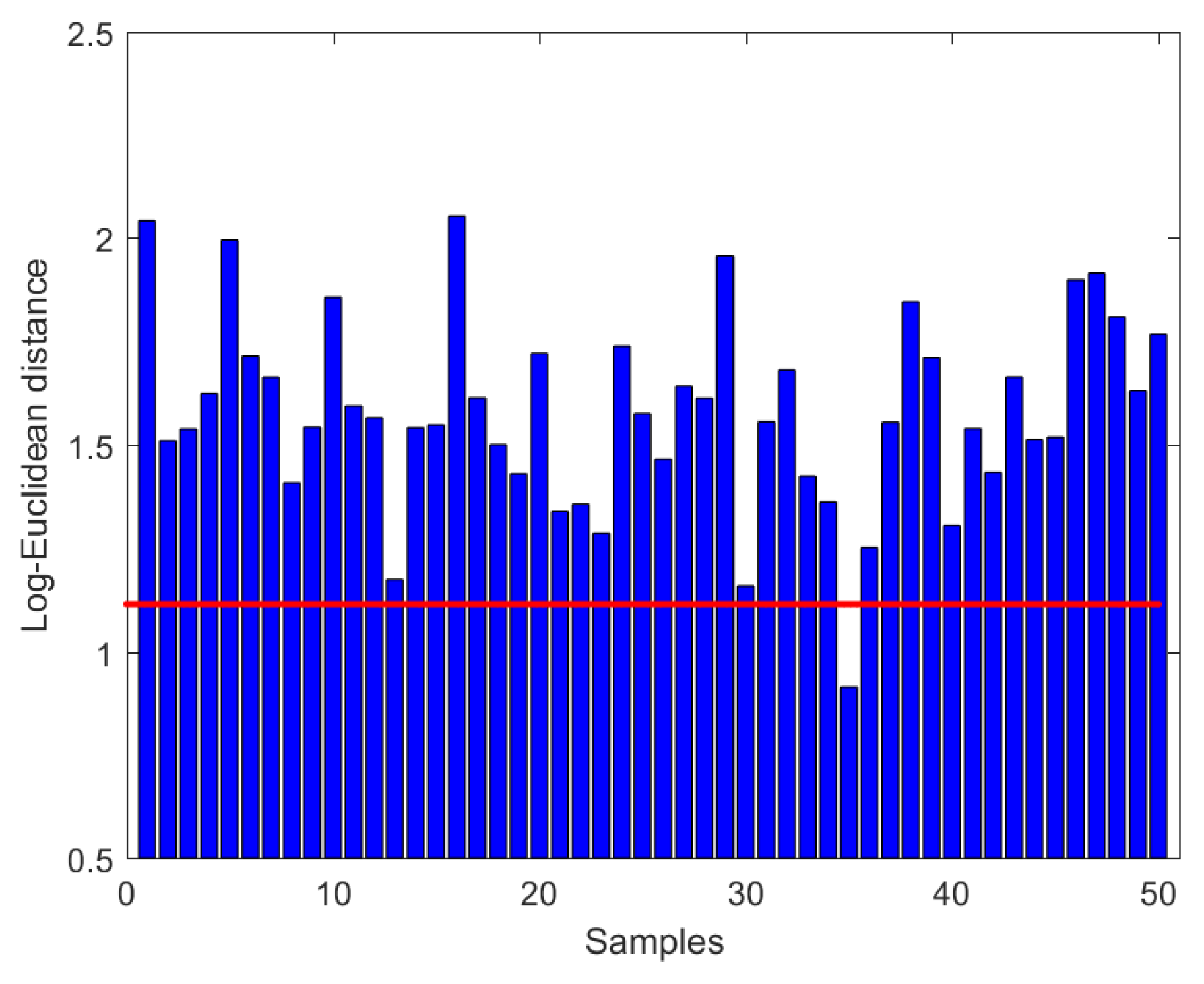
Example 2.

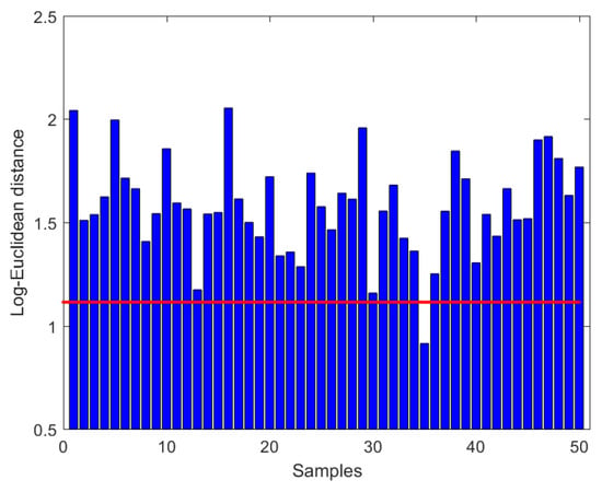
Let $n=5$ and $N=25$ in Theorem 1, 51 randomly generated samples on $P\left(5\right)$ are then employed to verify the effectiveness of our method. Figure 4 shows that the log-Euclidean distance between $R_0$ and the mean ${\mathbb{M}}_{LE}(R_i\backslash R_0))$ is 1.1141 (straight line) and the bar graphs denote the log-Euclidean distance from the log-Euclidean mean to each sample.

Figure 4. Log-Euclidean distance to samples.

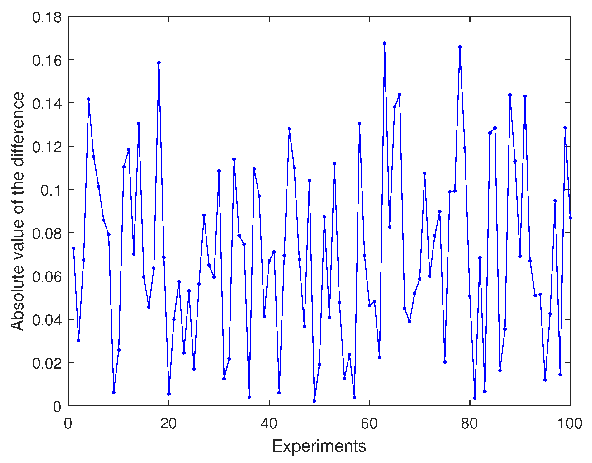
Then, we use 100 experiments to compare our method with that developed by Ref. [6]. Figure 5 shows that the absolute value $|d_{LE}(R_0,{\mathbb{M}}_{LE}(R_i\backslash R_0))-d_{Aff}(R_0,{\mathbb{M}}_{Aff}(R_i\backslash R_0))|<0.17.$ Moreover, our method is non-iterative, and the log-Euclidean framework is simpler than that of Ref. [6]. It is obvious that our approach is more time-efficient. Thus, we do not compare the computing time of the two methods in the above simulations.

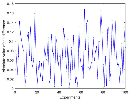
Figure 5. Absolute value of the difference gotten by two methods.

In conclusion, our non-iterative method in log-Euclidean framework is effective, and the calculation results are very close to those of the classical method proposed by Ref. [6].

Example 3.

In this example, the difference of means method is used to judge whether there are target matrices in detected matrices.

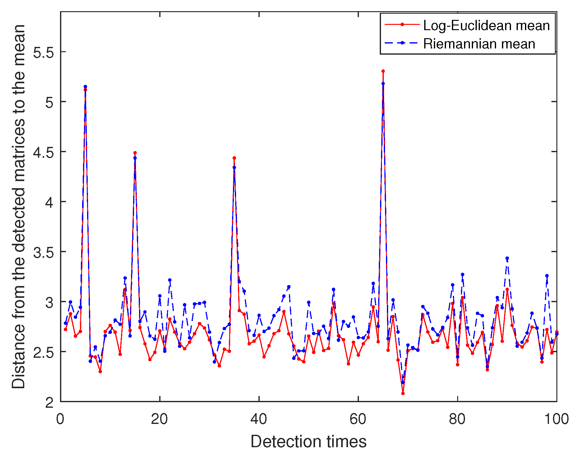
First, let $n=10$ and $N=20$, we could get 100 random detected matrices $R_0^1,\dots ,R_0^{100}$ and 40 randomly reference matrices $R_{-20},\dots ,R_{-1}$, $R_1,\dots ,R_{20}$ on $\mathrm{P}\left(10\right)$, where $R_0^5,R_0^{16},R_0^{35},R_0^{64}$ are obtained by adding $bI$$(2<b<3)$ to random symmetric positive-definite matrices matrices. For each detected matrix $R_0^j$, the distance between $R_0^j$ and the mean of the reference matrices is, respectively, calculated by our non-iterative method in Theorem 1 and the algorithm proposed by Ref. [6]. Figure 6 shows the distance curves produced by the two methods are in good agreement and $R_0^5,R_0^{16},R_0^{35},R_0^{64}$ can be clearly distinguished from the reference matrices. Then, similar to the above process, we set $n=2$ and display 100 randomly detected matrices ( circle) and 40 randomly reference matrices (blue asterisk) in XYZ system. In Figure 7, it is seen that $R_0^5,R_0^{16},R_0^{35}{R}_0^{64}$ (red circle) are far from the reference matrices. Consequently, our deference of means method is more valid to seek the target matrices than the algorithm developed by Ref. [6].

Figure 6. Distance from the detected matrices to the mean.

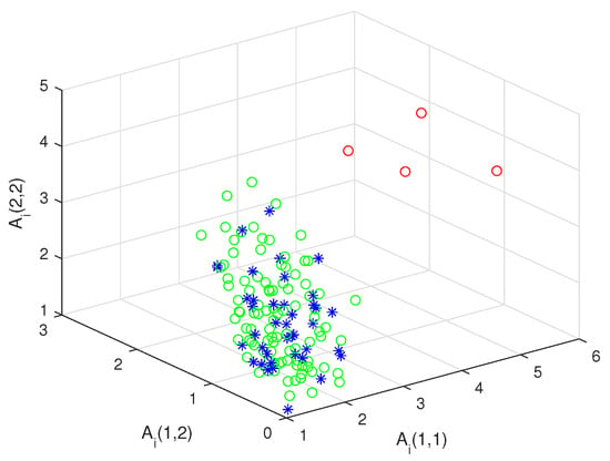
Figure 7. Target matrices.

4. Application to Point Cloud Denoising

In this section, the method for the difference of means is applied to denoise the point clouds with high density noise via the K-means clustering algorithm. When there is a considerable distance between data within a cluster, the traditional clustering algorithm will suffer from difficulties, making it difficult to distinguish the random noise from the effective data [21]. In Ref. [22,23], clustering is carried out according to the neighborhood density of each data. It is noted that the local statistical structures of noise and effective data are different, so the data with similar local statistics should be grouped into the same cluster. Afterwards, all point clouds are projected into the parameter distribution families to obtain the parameter point clouds, which contain the local information of the origin point cloud. Then, the original point cloud is classified according to the clustering results of the parameter point clouds.

4.1. Algorithm for Point Cloud Denoising

First, the original data point clouds are mapped to the normal distribution family manifolds, whose expectation and covariance matrix are calculated by the k-nearest neighbors of each point cloud, such that the parameter point clouds are formed. In ${\mathbb{R}}^n$, we denote the point clouds with scale l as

$$\mathcal{C}:=\{{\mathbf{p}}_i\in {\mathbb{R}}^n\mid i=1,\dots ,l\}.$$

(43)

For any $\mathbf{p}\in \mathcal{C}$, the k-nearest neighbor method is used to select the neighborhood $N(\mathbf{p},k)$, which is abbreviated as N. Then, the expectation $\mu \left(N\right):=E\left(N\right)-\mathbf{p}$ and covariance matrix $\mathsf{\Sigma }\left(N\right):=Cov\left(N\right)$ of the data points in N is calculated. Finally, the data points are represented as parameter points on an n-ary normal distribution family manifold $N_n$, where

$$N_n=\left\{P\right|P=P(\mathbf{x};\mu ,\mathsf{\Sigma })=\frac{1}{\sqrt{{\left(2\pi \right)}^n}det\left(\mathsf{\Sigma }\right)}exp\{-\frac{{(\mathbf{x}-\mu )}^T{\sum }^{-1}(\mathbf{x}-\mu )}{2}\}.$$

(44)

Thus, the local statistical mapping is defined by

$$\mathsf{\Psi }:\mathcal{C}\to N_n,$$

(45)

which satisfies

$$\mathsf{\Psi }\left(P\right)=P(\mu \left(N\right),\mathsf{\Sigma }\left(N\right))=\frac{1}{\sqrt{{\left(2\pi \right)}^n}det\left(\mathsf{\Sigma }\right)}exp\{-\frac{{(\mathbf{x}-\mu )}^T{\sum }^{-1}(\mathbf{x}-\mu )}{2}\}.$$

(46)

Under the local statistical mapping $\mathsf{\Psi }$, the image $\tilde{\mathcal{C}}:=\mathsf{\Psi }\left(\mathcal{C}\right)\subseteq N_n$ of the point cloud $\mathcal{C}$ is called the parameter point cloud [24]. The barycenter of the parameter point cloud $\tilde{\mathcal{C}}$ is defined as follows

$$\mathbf{c}\left(\tilde{\mathcal{C}}\right)=arg\underset{(\mu ,\mathsf{\Sigma })\in N_n}{min}\sum _{i=1}^l{d}^2(({\mu }_i,{\mathsf{\Sigma }}_i),(\mu ,\mathsf{\Sigma })).$$

(47)

Moreover, the barycenter $\mathbf{c}\left(\tilde{\mathcal{C}}\right)$, that is, the geometric mean, depends on the selection of the distance functions on $N_n$. To avoid the complex iterative calculation, the Euclidean distance (7) and the log-Euclidean distance (17) are used, respectively, in the following. Because $N_n$ and ${\mathbb{R}}^n\times \mathrm{P}\left(n\right)$ are topologically homeomorphic [25], the geometric structure on $N_n$ can be induced by defining the metrics on ${\mathbb{R}}^n\times \mathrm{P}\left(n\right)$. In one case, ${\mathbb{R}}^n\times \mathrm{P}\left(n\right)$ is embedded into ${\mathbb{R}}^n\times {\mathbb{R}}^{n\times n}$, the distance function on $N_n$ is obtained from the Euclidean metric

$$d_F(({\mu }_1,{\mathsf{\Sigma }}_1),({\mu }_2,{\mathsf{\Sigma }}_2))=\parallel {\mu }_1-{\mu }_2{\parallel }_F+{\parallel {\mathsf{\Sigma }}_1-{\mathsf{\Sigma }}_2\parallel }_F.$$

(48)

From (20), the geometric mean $\mathbf{c}\left(\tilde{\mathcal{C}}\right)$ is the arithmetic mean

$$\mathbf{c}\left(\tilde{\mathcal{C}}\right)=(\frac{1}{l}\sum _{i=1}^l{\mu }_i,\frac{1}{l}\sum _{i=1}^l{\mathsf{\Sigma }}_i).$$

(49)

Another case is to define the log-Euclidean metric (14) on $\mathrm{P}\left(n\right)$, then the distance function on $N_n$ is expressed as

$$d_{LE}(({\mu }_1,{\mathsf{\Sigma }}_1),({\mu }_2,{\mathsf{\Sigma }}_2))=\parallel {\mu }_1-{\mu }_2{\parallel }_F+{\parallel log\left({\mathsf{\Sigma }}_1\right)-log\left({\mathsf{\Sigma }}_2\right)\parallel }_F.$$

(50)

According to Lemma 1, the geometric mean $\mathbf{c}\left(\tilde{\mathcal{C}}\right)$ is the arithmetic mean in the logarithmic domain as follows

$$\mathbf{c}\left(\tilde{\mathcal{C}}\right)=(\frac{1}{m}\sum _{i=1}^l{\mu }_i,exp\{\frac{1}{m}\sum _{i=1}^{l}log\left({\mathsf{\Sigma }}_i\right)\}).$$

(51)

Note that the local statistical structure of signal is very different from that of random noise, so we will cluster $\tilde{\mathcal{C}}$ into two categories: signal and noise. Due to the statistical properties of the n-ary normal distribution parameter family, the efficiency of the algorithm depends on the selection of distance functions on $N_n$. Algorithm for clustering signal and noise is as follows.

In the process of clustering, Theorem 1 is used to calculate the log-Euclidean distance between the geometric mean of the category and each data point in the parameter point cloud $\tilde{\mathcal{C}}$. In addition, when clustering based on the distance function obtained by the log-Euclidean metric, the difference between the old and new barycenters is compared in the logarithmic domain to avoid calculating exponential mapping.

4.2. Numerical Examples

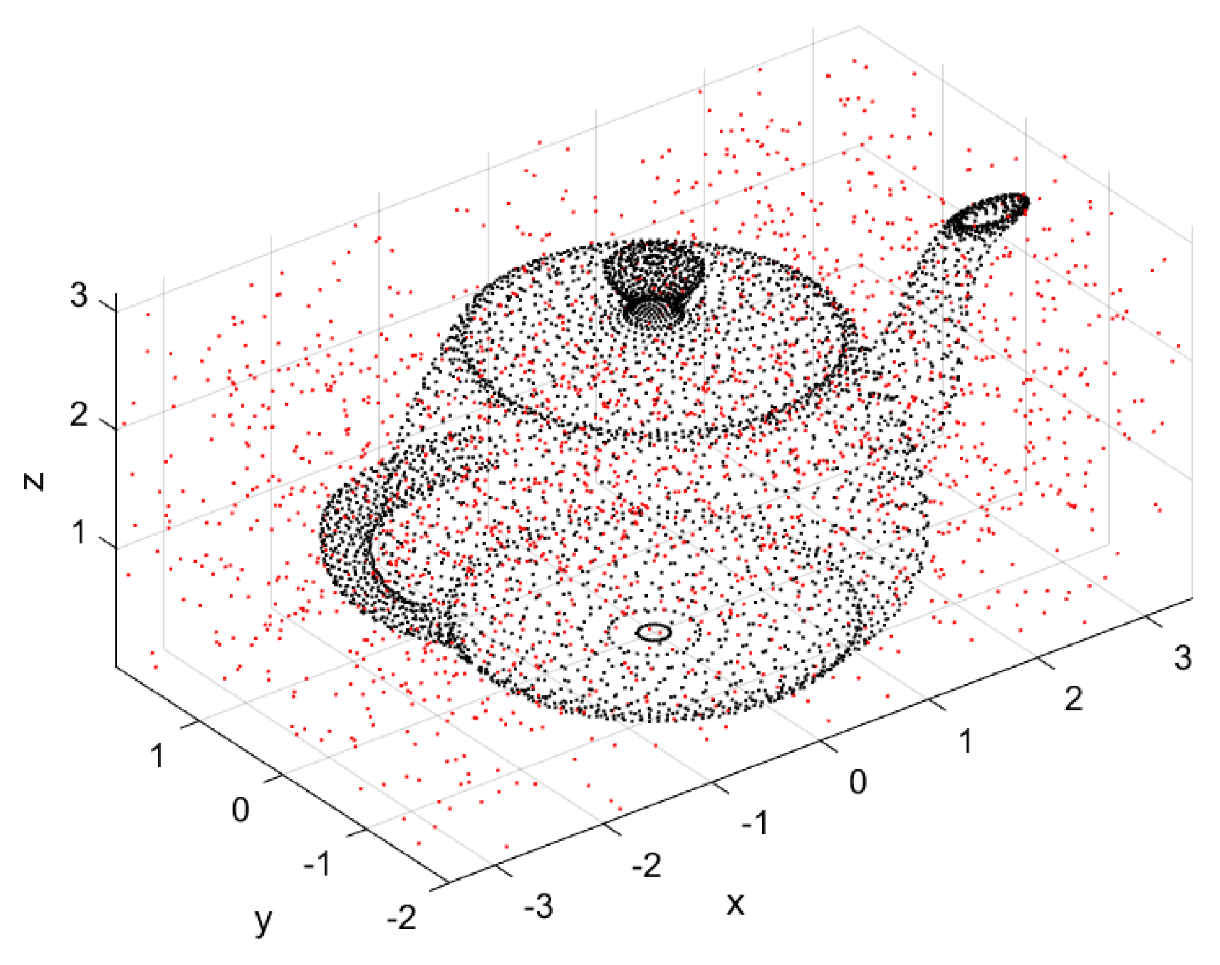
This subsection verifies the effectiveness of Algorithm 1 in removing high-density noise, and compares the denoising effect of the distance function obtained by the Euclidean metric and that of the log-Euclidean metric. The experimental data adopts the 3-dimensional point cloud of Teapot, and the background noise is uniformly distributed, where the signal-to-noise ratio (SNR) is 4148:1000, as shown in Figure 8.

Algorithm 1 Algorithm for clustering signal and noise.

Inputs: Point clouds $\mathcal{C}$, value of k and convergence threshold $\epsilon$. Output: Two categories of point clouds $\mathcal{C}$. Main loop: Map the point cloud $\mathcal{C}$ into a parameter point cloud $\tilde{\mathcal{C}}$. K-means algorithm (K = 2): set two barycenters of the current division as ${\mathbf{c}}_1^{\left(i\right)}$ and ${\mathbf{c}}_2^{\left(i\right)}$, and use the K-means algorithm based on the distance function (48) or (50) to cluster the parameter point cloud $\tilde{\mathcal{C}}$. Then, according to the clustering results, the geometric mean of each category is calculated by (49) or (51). Update two barycenters of the current division to the geometric mean ${\mathbf{c}}_1^{(i+1)}$ and ${\mathbf{c}}_2^{(i+1)}$. If $d({\mathbf{c}}_1^{\left(i\right)},{\mathbf{c}}_1^{(i+1)})<\epsilon$ and $d({\mathbf{c}}_2^{\left(i\right)},{\mathbf{c}}_2^{(i+1)})<\epsilon$, two categories of the original point cloud $\mathcal{C}$ is output according to the current division of the parameter point cloud $\tilde{\mathcal{C}}$. Otherwise, proceed to step 2.

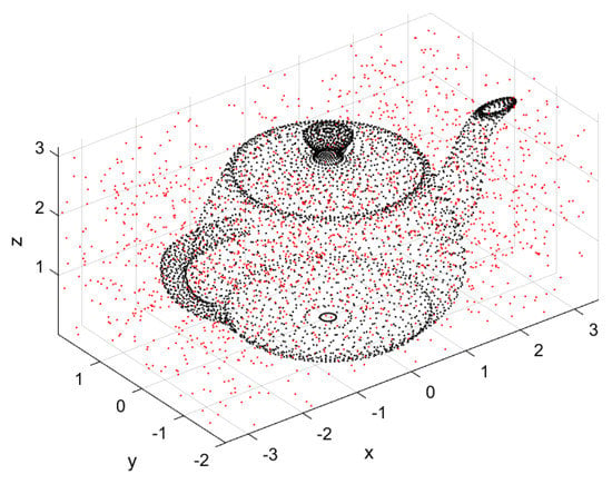
Figure 8. Original data cloud.

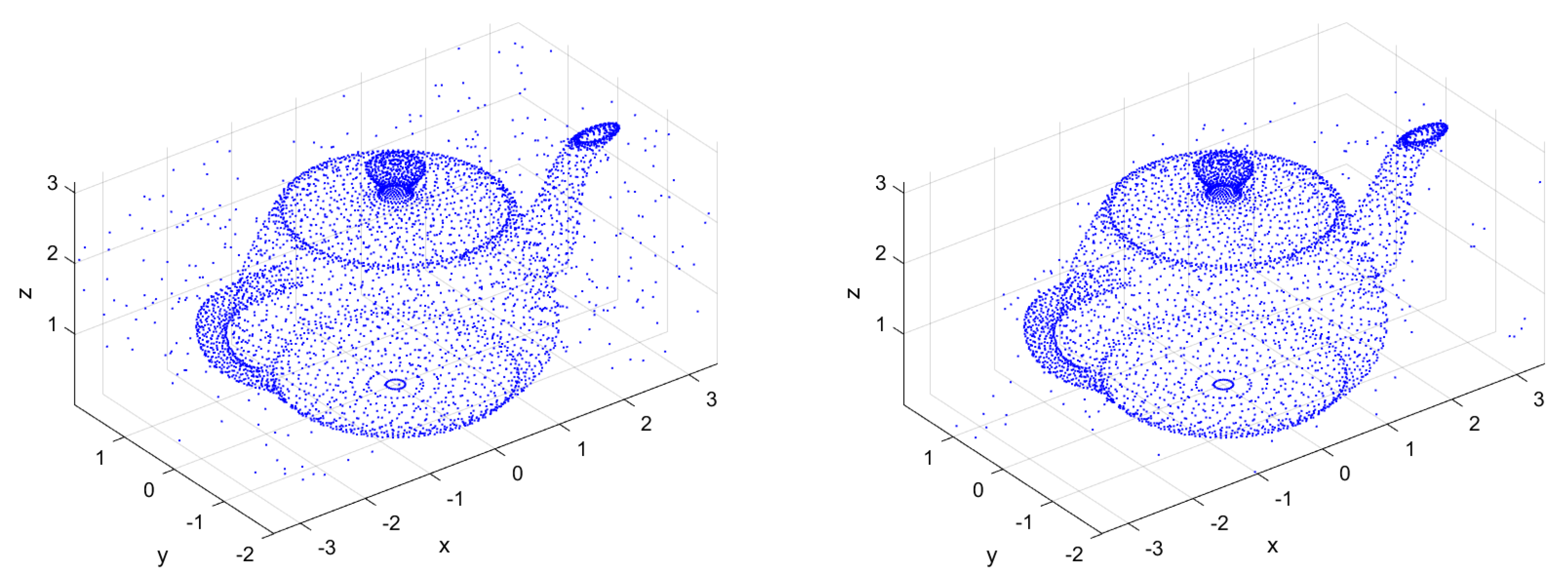
Take $k=5,K=2$ and $\epsilon =0.01$, Figure 9 is the denoised images of the original point cloud by Algorithm 1, based on the Euclidean metric and the log-Euclidean metric, respectively. Obviously, Algorithm 1 based on the log-Euclidean metric is more effective.

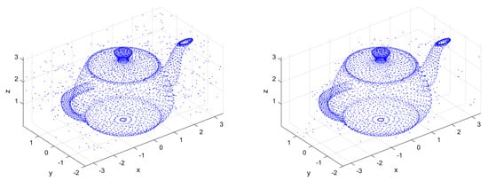
Figure 9. Point cloud after denoising based on Euclidean metric (left) and log-Euclidean metric (right).

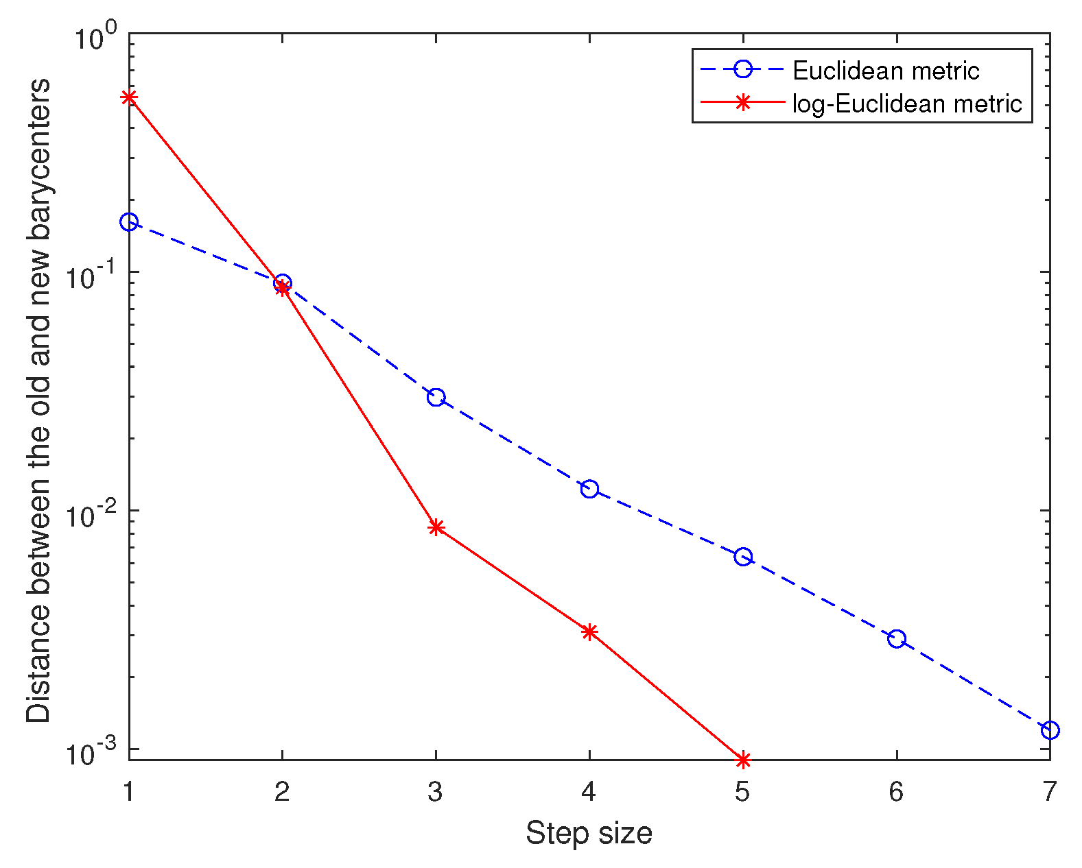
The efficiency and the convergence of Algorithm 1 is shown by Figure 10. It also demonstrates that Algorithm 1 using the log-Euclidean metric has faster convergence speed. To compare the denoising effects of different metrics, we adopt three criteria: Accuracy, Recall and Precision. For different SNR, the experimental results are shown in Table 1. In conclusion, Algorithm 1 based on the distance obtained by the log-Euclidean metric has obvious denoising effect for high-density noise, which is a successful application of our proposed method (Theorem 1). Furthermore, it is proved again that the Euclidean metric can not well describe the geometric structure on manifolds.

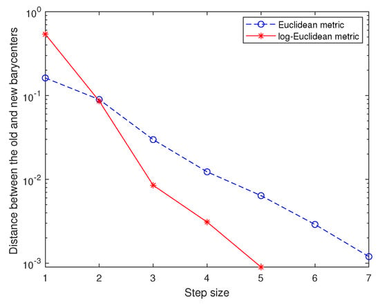
Figure 10. Denoising effects of different metrics (log scale).

Table 1. Comparison of denoising effects.

Metric	SNR 4148:1000			SNR 4148:2000
	Precision	Recall	Accuracy	Precision	Recall	Accuracy
log-Euclidean metric	91.53%	100%	92.54%	85.35%	99.45%	88.11%
Euclidean metric	85.41%	99.88%	86.15%	74.40%	93.66%	73.98%

5. Conclusions

On the Lie group of symmetric positive-definite matrices, we present a non-iterative method to calculate the distance between a matrix and the mean matrix. Based on log-Euclidean metrics, we transform computations on the Lie group into computations on the space of symmetric matrices in the domain of matrix logarithms, and obtained the conclusion that this distance can be represented by the Euclidean distance between the right weighted mean and the left weighted mean. Our proposed method is simpler and more efficient than the classical iterative approach induced by affine-invariant Riemannian metrics in Ref. [6]. In addition, one example shows that the log-Euclidean mean and the Riemannian mean are more suitable than the arithmetic mean on the space of symmetric positive-definite matrices, and the other two examples illustrate that our method in Theorem 1 is more effective than the approach developed by Ref. [6]. Finally, the method for the difference of means is applied to denoise the point clouds with high density noise via the K-means clustering algorithm, and the experimental results show that Algorithm 1, which is based on the distance induced by the log-Euclidean metric has an obvious denoising effect.

References

- Agarwal, M.; Gupta, M.; Mann, V.; Sachindran, N.; Anerousis, N.; Mummert, L. Problem determination in enterprise middleware systems using change point correlation of time series data. In Proceedings of the 2006 IEEE/IFIP Network Operations and Management Symposium NOMS 2006, Vancouver, BC, Canada, 3–7 April 2006; pp. 471–482. [Google Scholar]
- Cheng, Y.; Wang, X.; Morelande, M.; Moran, B. Information geometry of target tracking sensor networks. Inf. Fusion 2013, 14, 311–326. [Google Scholar] [CrossRef]
- Li, X.; Cheng, Y.; Wang, H.; Qin, Y. Information Geometry Method of Radar Signal Processing; Science Press: Beijing, China, 2014. [Google Scholar]
- Merckel, L.; Nishida, T. Change-point detection on the lie group SE(3). In Proceedings of the International Conference on Computer Vision, Imaging and Computer Graphics, Angers, France, 17–21 May 2010; Springer: Berlin, Germany, 2010; pp. 230–245. [Google Scholar]
- Arnaudon, M.; Barbaresco, F.; Yang, L. Riemannian medians and means with applications to Radar signal processing. IEEE J. Sel. Top. Signal Process. 2013, 7, 595–604. [Google Scholar] [CrossRef]
- Barbaresco, F. Interactions between Symmetric Cone and Information Geometries: Bruhat-Tits and Siegel Spaces Models for High Resolution Autoregressive Doppler Imagery, Emerging Trends in Visual Computing; Springer: Berlin, Germany, 2008. [Google Scholar]
- Duan, X.; Zhao, X.; Shi, C. An extended Hamiltonian algorithm for the general linear matrix equation. J. Math. Anal. Appl. 2016, 441, 1–10. [Google Scholar] [CrossRef]
- Luo, Z.; Sun, H. Extended Hamiltonian algorithm for the solution of discrete algebraic Lyapunov equations. Appl. Math. Comput. 2014, 234, 245–252. [Google Scholar] [CrossRef]
- Chen, W.; Chena, S. Application of the non-local log-Euclidean mean to Radar target detection in nonhomogeneous sea clutter. IEEE Access 2019, 99, 36043–36054. [Google Scholar] [CrossRef]
- Wang, B.; Hu, Y.; Gao, J.; Ali, M.; Tien, D.; Sun, Y.; Yin, B. Low rank representation on SPD matriceswith log-Euclidean metric. Pattern Recognit. 2016, 76, 623–634. [Google Scholar] [CrossRef]
- Liu, Q.; Shao, G.; Wang, Y.; Gao, J.; Leung, H. Log-Euclidean metrics for contrast preserving decolorization. IEEE Trans. Image Process. 2017, 26, 5772–5783. [Google Scholar] [CrossRef]
- Moakher, M. A differential geometric approach to the geometric mean of symmetric positive-definite matrices. SIAM J. Matrix Anal. Appl. 2005, 26, 735–747. [Google Scholar] [CrossRef]
- Moakher, M. On the averaging of symmetric positive-definite tensors. J. Elast. 2006, 82, 273–296. [Google Scholar] [CrossRef]
- Batchelor, P.G.; Moakher, M.; Atkinson, D.; Calamante, F.; Connelly, A. A rigorous framework for diffusion tensor calculus. Magn. Reson. Med. 2005, 53, 221–225. [Google Scholar] [CrossRef] [PubMed]
- Arsigny, V.; Fillard, P.; Pennec, X.; Ayache, N. Log-Euclidean metrics for fast and simple calculus on diffusion tensors. Magn. Reson. Med. 2006, 56, 411–421. [Google Scholar] [CrossRef]
- Curtis, M.L. Matrix Groups; Springer: Berlin, Germany, 1979. [Google Scholar]
- Jost, J. Riemannian Geometry and Geometric Analysis, 3rd ed.; Springer: Berlin, Germany, 2002. [Google Scholar]
- Jorgen, W. Matrix diferential calculus with applications in statistics and econometrics. De Economist 2000, 148, 130–131. [Google Scholar]
- Fiori, S. Learning the Fréchet mean over the manifold of symmetric positive-definite matrices. Cogn. Comput. 2009, 1, 279–291. [Google Scholar] [CrossRef] [Green Version]
- Duan, X.; Sun, H.; Peng, L. Application of gradient descent algorithms based on geodesic distances. Sci. China Inf. Sci. 2020, 63, 152201:1–152201:11. [Google Scholar] [CrossRef] [Green Version]
- Jain, A.K. Data clustering. 50 years beyond K-means. Pattern Recognit. Lett. 2010, 31, 651–666. [Google Scholar] [CrossRef]
- Zhu, Y.; Ting, K.M. Carman, M.J. Density-ratio based clustering for discovering clusters with varying densities. Pattern Recognit. 2016, 60, 983–997. [Google Scholar] [CrossRef]
- Rodriguez, A.; Laio, A. Clustering by fast search and find of density peaks. Science 2014, 334, 1492–1496. [Google Scholar] [CrossRef] [PubMed] [Green Version]
- Sun, H.; Song, Y.; Luo, Y.; Sun, F. A clustering algorithm based on statistical manifold. Trans. Beijing Inst. Technol. 2021, 41, 226–230. [Google Scholar]
- Amari, S. Information Geometry and Its Applications; Springer: Tokyo, Japan, 2016. [Google Scholar]
Publisher’s Note: MDPI stays neutral with regard to jurisdictional claims in published maps and institutional affiliations. |
© 2022 by the authors. Licensee MDPI, Basel, Switzerland. This article is an open access article distributed under the terms and conditions of the Creative Commons Attribution (CC BY) license (https://creativecommons.org/licenses/by/4.0/).