Expect: EXplainable Prediction Model for Energy ConsumpTion

Abstract

With the steady growth of energy demands and resource depletion in today’s world, energy prediction models have gained more and more attention recently. Reducing energy consumption and carbon footprint are critical factors for achieving efficiency in sustainable cities. Unfortunately, traditional energy prediction models focus only on prediction performance. However, explainable models are essential to building trust and engaging users to accept AI-based systems. In this paper, we propose an explainable deep learning model, called Expect, to forecast energy consumption from time series effectively. Our results demonstrate our proposal’s robustness and accuracy when compared to the baseline methods.

1. Introduction

We changed footnote format throughout paper, please confirm. The rapid burgeoning of energy needs and technological developments have rocketed power consumption. In this respect, smart meters, which are electronic devices that provide real-time record energy consumption, increasingly replacing traditional electric meters. In 2019, according to the IoT Analytics report (https://iot-analytics.com/product/smart-meter-market-report-2019-2024/, accessed on 17 November 2021), the global penetration rate of smart meters is $41.2$%, which is expected to rise to nearly 59% by 2028. This transition was accompanied by an urgent need to modernize and enhance energy systems to reach sustainable development goals. Thus, an increasing number of research communities and industrial partners have taken up the challenge of analyzing smart meter data and proposing models to predict energy consumption. Moreover, it is worth mentioning that, since electricity is simultaneously consumed as it is generated at the power plant, it is pivotal to accurately predicting the energy consumption in advance for a stable power supply. Besides, in energy consumption, we are used to relying on the most efficient—either machine or deep learning-based—predictive models to unveil valuable knowledge towards gainful insights. Notwithstanding, a common criticism of such models is that their decision-making process is a “black box”; it is tricky to grasp how an algorithm makes a particular decision since most focus on performance and accuracy, vastly overlooking the explainability aspect. On the other hand, explainable Artificial Intelligence (XAI) is a growing facet of technical Al development in which humans can understand the solution results. In energy consumption, there is no more room for unquestionably relying on black-box system decisions whenever companies are hardly working on providing a personalized supportive role via virtual agents.

In this paper, we introduce the Expect framework (the Expect acronym stands for EXplainable Prediction model for Energy ConsumpTion), which relies on a deep learning-based technique to unveil the consumption patterns from the time-series data. The most challenging task is the feature engineering step, during which we have been facing a considerable amount of missing values. Acting the furthest from a random completion, we provide a new technique that extensively uses external information that makes the dataset reliable for the knowledge-building process. In addition, we also pay attention to the explainability of the provided predictions to make the latter more trusted by end-users.

We organize the rest of this paper as follows: Section 2 scrutinizes the wealth of works done so far in the field of energy consumption prediction. Section 3 painstakingly describes the introduced Expect framework. Then, we report the results of the experiments in Section 4. Finally, we conclude the paper and identify avenues for future work in Section 5.

2. Scrutiny of the Related Work

Time series forecasting has been deeply investigated in the literature for a decade. The primary purpose of this research field is to discover significant characteristics from the time-series data that can be used for forecasting future values. As a result, a myriad of research using time series forecasting has been proposed in different areas, including marketing, finance, and energy consumption [1,2,3]. This study presents a comprehensive review of the most pioneering approaches in the literature dealing with energy consumption prediction. We can identify two major streams: (i) Standalone models, which apply to a single technique; and (ii) Hybrid models, which integrate more than one standalone technique. Table 1 shows the abbreviations which will be used in the related work. We summarize the most recent studies in Table 2. In the following, we detail these categories.

Table 1. List of abbreviations. The abbreviations including in the text are reported alphabetically.

Abbreviation	Full form
AE	AutoEncoder
ARIMA	AutoRegressive Integrated Moving Average
ARMA	Autoregressive Moving Average
ANN	Artificial Neural Network
CNN	Convolutional Neural Network
EA	Evolutionary Algorithm
LR	Linear Regression
LSTM	Long Short-Term Memory
RT	Regression Tree
SVR	Support Vector Regression
XGboost	eXtreme Gradient Boosting

Table 2. Related works on time series energy forecasting.

Category	Reference	XAI	Statistical Techniques			Machine Learning Techniques					Deep Learning Techniques
			LR	ARMA	ARIMA	ANN	XGBoost	SVR	EA	RT	CNN	LSTM	AE
Standalone	[4]	No		×	×
	[5]	No	×
	[6]	No				×
	[7]	No										×
	[8]	No						×
	[9]	No					×
	[10]	Yes											×
Hybrid	[11]	No			×	×
	[12]	Yes									×	×
	[13]	No				×			×
	[14]	No			×			×	×
	[15]	No			×		×
	[16]	Yes	×							×

2.1. Standalone Models

Based on the techniques, we split standalone models into three categories: statistical, machine learning, and deep learning.

2.1.1. Statistical Techniques

Several conventional statistical models have been widely used in non-linear time series forecasting problems and have shown their outstanding performance in energy consumption forecasting. In this paper, we focus on the most recently used approaches, such as linear regression (LR), autoregressive moving average model (ARMA), and autoregressive integrated moving average model (ARIMA).

The ARMA model is one of the most popular univariate models in stationary random sequence analysis since it combines the advantages of the autoregressive and the moving average models [17]. However, in real life, most time series are non-stationary. The ARIMA model overcomes this limitation by introducing a differencing process. According to [18], the proposed approach models stationariness and trend in time series data, considering both autoregressive and mobile environments. In this respect, the authors in [4] performed a comparative study between ARIMA and ARMA models for household electric consumption. The used data in the different models were collected in the period ranging from December 2006 to November 2010. Based on their results, the authors concluded that the ARIMA model is more suitable for monthly and quarterly forecasting. In contrast, the ARMA model is likely appropriate for daily and weekly forecasting. In the same study, the authors conducted other evaluations using the linear regression analysis, which relies on causal relationships, one of the statistical methods used for energy consumption forecasting in buildings. In another study, the authors applied a single and multiple linear regression analysis on hourly and daily data to predict the energy consumption in the residential sector [5]. The authors have proven that the time resolution of the observed data has a relevant impact on the prediction performance.

2.1.2. Machine Learning Techniques

Machine learning methods have been increasingly used to tackle time series forecasting problems. Some studies proposed artificial neural networks (ANNs) for energy demand prediction and optimization. For instance, Beccali et al. integrated a two-layer ANN with multilayer perceptron in a decision-making tool that provides fast forecasting of the energy consumption in commercial and educational buildings [6]. They identified the most suitable architectures of two ANNs by the data provided from the energy audits of 151 public buildings in four regions of South Italy. In their proposed framework, the first ANN provided the actual energy performance building, while they dedicated the second ANN to evaluating the best refurbishment actions. Both of them were trained on an extensive set of data and provided good performance. In another study, Aslam et al. pointed out that, although ANN models have good learning capability, it often causes underfitting and over-fitting problems [19]. Another widely explored technique in time series forecasting is the SVR model. In this respect, Zhong et al. developed an efficient vector field-based SVR method aimed to establish an energy consumption prediction model [8]. Their approach was based on a multi-distortion of feature space which eliminates the high nonlinearity of the dataset. In the same study, the authors mentioned that their improved algorithm enhanced the performance of SVR from three aspects, including prediction accuracy, robustness, and generalization capabilities. In another study, the XGBoost model has been used to construct a prediction model to forecast electricity load [9]. The authors outlined that their model can capture the non-linear relationships in a small-scale dataset provided by the Australian Energy Market Operator (AEMO). Their approach increased the number of features by converting daily data into weekly data and then applied XGboost for feature selection. As a result, they recorded good performance on monthly predictions. However, the authors also reported that the XGboost did not perform well with high electricity loads. The obtained results were presented without being compared to alternative approaches.

2.1.3. Deep Learning Techniques

Deep learning, which is a rising method to solve complex tasks, has shown promising results in different areas for prediction purposes [20]. In recent years, deep architectures have been extensively used to address the energy consumption prediction problem [10]. In this respect, Kong et al. presented a system to forecast the short-term energy consumption using deep learning techniques [7]. The proposed system takes advantage of the ability of the long short-term memory (LSTM) recurrent neural network to learn the long-term temporal dependencies and tendency relationships. Furthermore, the authors performed a comparative study using a publicly available set of real residential smart meter data with the existing prediction methods. As a result, their proposed approach outperforms its competitors in short-term load forecasting. Another study carried out by Kim et al. [10] lies in the same trend. The authors built an explainable deep learning model to predict household electricity consumption for 15, 30, 45, and 60 min resolutions. Their proposed model proceeds as follows: based on the energy demand, the projector defines the current demand pattern, called a state, from which the predictor predicts the future energy demand. Thus, various explanations are given besides predictions. The experimental results show high and stable performance on very complex data of 5 years compared with previous studies.

Most of the models for time series forecasting have rarely been used alone in the literature. They tried to combine the advantages of different predictive models to have more accurate and reliable forecasts. These are called hybrid models. In the following, we will describe some of these approaches.

2.2. Hybrid Approaches

Hybrid models can deal with real-world problems, often complex. A single machine learning model may not capture the complexities of energy and operational data. For instance, the study carried in [11] focuses on the benefit of using two widely popular and effective forecasting models, that is, ARIMA and ANN. According to the authors, a real-world time series combines linear and nonlinear components. After a prior decomposition of the series into low and high-frequency signals, they apply the ARIMA and ANN models separately. Hence, the stationarity and linearity of the load is handled by the ARIMA model, and the residual error is described by ANN, which fits the nonlinear characteristic. Similarly, other methods can be combined to improve forecasting accuracy. Kim and Cho presented an efficient CNN-LSTM neural network for time series energy forecasting [12]. The authors pointed out that the CNN layer can extract the features between several energy consumption variables. The LSTM layer is appropriate for modeling temporal information of periodic trends in time series components. In another study, an improved adaptive neuro-fuzzy inference system for hourly near-real-time predictions of energy consumption was introduced [13]. The authors proposed a new version of the swarm-based meta-heuristic firefly algorithm to improve their hybrid machine learning approach. The robustness of the developed model was tested on a public dataset containing six commercial buildings located in different sites. Other studies combined different machine learning techniques [14]. In their proposed model, the authors adopted linear (ARIMA and SVR) and nonlinear methods (GA) to enhance the prediction accuracy. As a result, the integrated framework performs well on the Taiwanese primary energy consumption dataset. The authors confirm that hybrid models can model complex autocorrelation structures in the data more accurately. Later, Yucong and Bo proposed the EA-XGboost framework, which relies on ARIMA and XGboost models to predict building energy consumption [15]. First, the ARIMA model is applied to each Intrinsic Mode Functions (IMF) generated from the time series data. Afterwards, the XGboost model processes the result as a feature with other energy-related factors. Recently, Ilic et al. proposed an explainable boosted linear regression (EBLR) algorithm for time-series forecasting [16]. Their iterative model operates into two phases: In the first phase, a base model, such as linear regression, is trained to obtain the preliminary forecasts. Then, a set of rules is identified by a regression tree through a feature generation based on residual exploration in the second phase. This process creates a single and interpretable feature to the base model to improve its performance. Results reveal that the proposed method achieves the best forecasting accuracies.

2.3. Discussion

The above-mentioned state-of-the-art techniques have been successfully applied to energy consumption forecasting. However, each technique has certain advantages and should be appropriately applied to a specific case. In the following, we shed light on the benefits and limitations of each technique discussed previously.

Prominent different statistical methods have been widely used for time series forecasting. The main reason for this success is their robustness and flexibility. Moreover, these methods rely on simplifying the expected task for the model by considering a priori knowledge and performing well with limited data availability. Nevertheless, some weaknesses have been found in the literature, the main one being missing nonlinearity. The essential cons of these models stand in the fact that they groundlessly assume linear relationships between past values. Unfortunately, this is not always the case with real-world data, thence inhibiting prediction performance [3]. Furthermore, these methods are most suitable for only short and medium ranges [21].

Later, machine learning techniques were proposed to overcome the limits of statistical methods. Their primary benefit stands in capturing the nonlinear patterns of the series. For instance, as mentioned in [8], SVR performs well for small datasets and can maintain a good generalization ability. However, although machine learning methods successfully overcome the drawback of statistical models in nonlinear relationships, they can yield, sometimes, a dull performance for purely linear time series [11].

Recently, deep learning methods have proved their accuracy and computational relevance. They can abstract features by creating a synthesis of different nonlinear transformations. Besides that, these methods can approximate almost any continuous function and can extract cross-series information for features to enhance individual forecasting. Besides these strengths, deep learning methods face several limitations. Apart from demanding vast amounts of data and extensive computational times, methods based on deep learning have difficulties when extrapolating data [19].

To summarize, we cannot assume that a technique is universally suitable to model a real-world time series. The selection of a forecasting method depends on data availability and the defined objectives. Therefore, it is of paramount importance to understand the time series before conducting a forecast. Besides, any forecasting method has its unique strengths and limitations. Therefore, a significant part of the success lies in choosing the appropriate method for the forecasting problem.

3. Expect: EXplainable Prediction Model for Energy ConsumpTion Framework

This section thoroughly describes our proposed framework for predicting and explaining energy consumption. We use a dataset (https://ieee-dataport.org/competitions/fuzz-ieee-competition-explainable-energy-prediction#files, accessed on 17 November 2021) that was made available by the Fuzz-IEEE competition on explainable energy prediction [22]. The Expect framework provides accurate predictions for 3248 smart meters upon the one-year data. It is worth mentioning that dealing with this dataset was the furthest from a straightforward task because of many missing values. To give a mouthwatering illustration of the missing value rate: on average, the consumption dataset contains 51.62% of missing values. Note, moreover, that the missing values are not equally distributed over the smart meters. For instance, the worst smart meters have only $2.47\%$ of data available, whereas the best one has $98.91\%$. The concept of missing values is a significant issue in many real-world datasets, yet there are no standard methods for dealing with it appropriately. Thus, it is crucial to understand how to overcome this challenge to manage data and generate a robust model successfully. We propose several imputation algorithms designed to deal with the different missing values appearing in our datasets. After this explanatory data analysis step, the Expect prediction model aggregates both consumption and weather information and feeds them to the embedding proposed layers in order to extract the temporal and environmental hidden features. Afterwards, we establish an LSTM-based neural network model to forecast energy consumption. The energy consumption values generated by our model are evaluated and analyzed by several error metrics. Finally, to increase our model’s trust, we rely on an agnostic method (ad-hoc and causality-based) to explain the generated predictions. However, towards scalability, the embedding layer in our system makes us lose the traceability of the original features. Thus, none of the well-known explainability frameworks (LIME, SHAPE) can be applied. One solution for this problem was to use the graphical interpretation for the explanation. Therefore, we chose the partial dependence plot (PDP) method [23], which shows the marginal effect that one or two features have on the predicted outcome of a machine learning model. This method is mainly based on interpreting the generated plots.

The overall architecture of our framework, depicted by Figure 1, puts forward four key steps: (a) Exploratory data analysis; (b) Feature engineering; (c) Model training; and (d) Prediction & Explainability. In the following, we detail the distinct steps of the workflow:

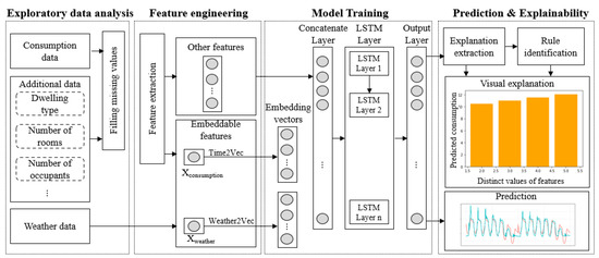
Figure 1. The overall architecture of the proposed framework.

3.1. Exploratory Data Analysis

We usher the process by inspecting the dataset to get an overview of some issues that may occur on real data, such as outlying observations, missing values, and other messy features, to name but a few. As shown in Figure 1, distinct types of data were provided:

• Consumption data: Historical half-hourly energy readings for 3248 smart meters having a different range of months’ worth of consumption. The available data for a given (fully anonymized) meter_id may cover only one month or more during the year.
• Additional data: Some collected additional information was made available for a subset of the smart meters. Indeed, only 1859 out of 3248 contain some additional information, including: (a) categorical variables: dwelling type for 1702 smart meters, heating fuel for 78 smart meters, hot water fuel for 76 smart meters, boiler age for 74 smart meters, etc.; and (b) numerical variables: number of occupants for 74 smart meters, number of bedrooms for 1859 smart meters, etc.
• Weather data: Daily temperature associated with 3248 smart meters, including the average, minimum, and maximum temperature values, respectively. The location and the postcode/zip code were anonymized for privacy issues.

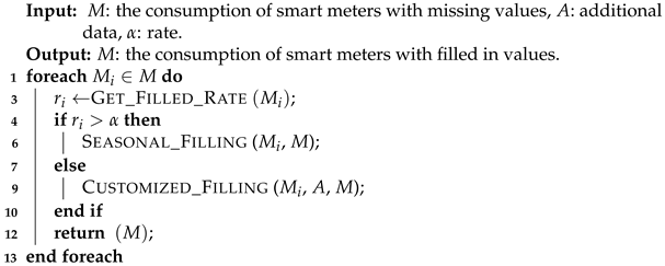
The most thriving and challenging issue with this dataset is that both the energy and additional information data contain a non-trivial amount of missing values, requiring an effective method of filling those values. Thus, our framework relies on an efficient algorithm that we introduce to fill appropriately in the incomplete data. In a first step, we propose an algorithm whose pseudo-code is sketched by Algorithm 1 to fill in missing values of the consumption data. The algorithm starts by checking the rate of missing values for each smart meter through the Get_Filled_Rate function (line 3). We then compared that rate to a pre-defined threshold $\alpha$, set equal to $0.6$ in our case (line 4). Finally, according to the rate threshold, we filled in the missing values with either the Seasonal_Filling procedure (line 6) or the Customized_Filling procedure (line 9).

Algorithm 1: Filling missing data for consumption.

In the following, we thoroughly describe the above routines. Thus, the pseudo-code of the Seasonal_Filling procedure is shown by Algorithm 2. The latter requires a prior of the time series based on the weather data. Thus, we identified 4 distinct energy-temperature regimes (seasons) according to Figure 2:

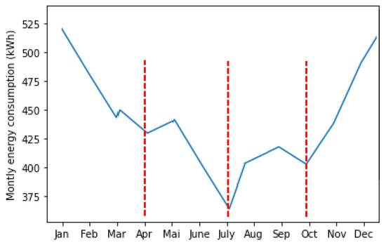
Figure 2. Average monthly energy consumption by year.

• Season 1: This is defined from January to the end of March (beginning of April). This season is flagging out gradually, decreasing energy consumption;
• Season 2: It runs from April to June (beginning of July). During this season, energy consumption tends to decrease. The shape of the plot indicates a decrease in energy consumption starting from May to June. In addition, the temperature in this season tends to increase;
• Season 3: It goes from July to September (beginning of October). We identify frequent but more minor energy variations during this season compared to season 2, growing as temperature increases;
• Season 4: It covers October to the end of December. Frequent and large energy fluctuations characterize it, with relatively large mean consumption. As a rule of thumb, the temperature is decreasing in this season.

Algorithm 2: Seasonal_Filling ($M_i$, M).

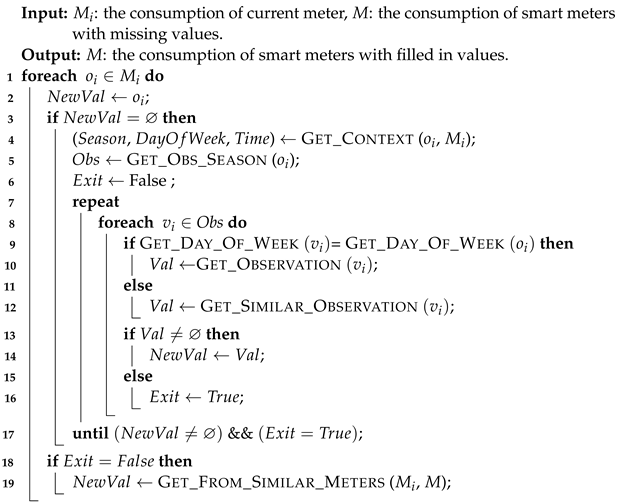In this study, the consumption dataset was given in 30-min intervals; 24 h apart corresponds to 48 time-steps and 12 h to 24 time-steps, and so forth. We tried to identify cyclical patterns in the time series based on statistical analysis. Informally, autocorrelation is the similarity between observations due to the time lag between them. Looking closely at Figure 3, we distinguish a sinusoidal shape. The following observations are worth underscoring: The energy consumption for a particular hour, each day, is most strongly correlated to the same hour of the day before or after. This relationship weakens as the number of days increases but peaks again 1 week apart (336 time-steps). According to the provided autocorrelation values, this value has a stronger correlation than 1 day apart. The Seasonal_Filling procedure starts by getting all observations related to a given meter across the year. For each missing value, the Get_Context depicts its context, which refers to the season (season 1, season 2 and season 3), the day of the week (Monday, Tuesday, etc.), and the daily time range (AM and PM) (line 4). Afterward, the Get_Obs_Season returns the list of observations $Obs$ in the same season as the considered missing value $o_i$ (line 5). For each element of the list $Obs$, the imputation of the missing value is assessed through the Get_Observation function in case we have the same day of the week and time range (line 10). Otherwise, the missing value is filled in via the Get_Similar_Observation function, which provides a similar observation in the same week and time range (line 12). In the case where we still have missing values, the Get_From_Similar_Meters function imputes the value based on the most akin smart meters (line 24). The Customized_Filling procedure, whose pseudo-code is shown by Algorithm 3, proceeds vertically (unlike the Seasonal_Filling procedure) and is applied to the smart meters having a filling rate less than $\alpha$. In this procedure, we deal with an enormous amount of missing data. Some observations only cover about 7% of the total data, to name but a few. The basic idea of the Customized_Filling procedure is to assign values according to the similarity between smart meters. After identifying the missing range of data, for a given smart meter $M_i$, through the Get_Missing_Ranges function (line 2) akin to smart meters with filled-in values, are gathered for each range through the Get_Sim_Meters function (line 4). To wrap up the process, the Update_Meters procedure fills in the missing ranges according to the most similar smart meters (line 5). The Customized_filling procedure distinguishes the type of day (weekend/weekday). Replaced with data from the nearest type of day, they allude more accurately to how a data pattern changes over time. In a second step, we propose two methods to fill the missing values of the additional data. Because of the large number of missing values in this dataset, which exceeds 96% for most features, we decided to keep only the following features: dwelling_type and num_bedrooms with, respectively, $20.58$% and $13.25$% of missing values. One proposed method is depicted by Algorithm 4. Here, we get the N similar meters according to the consumption data through the Get_Meters function (line 3). After that, we call the Get_Similarity function iteratively to assess the similarity between the N meters to find the most similar one (line 6–11). The second method is described by Algorithm 5. Finally, we perform clustering on the meters by calling the Meter_Clustering function based on both consumption and available features from additional information dataset (line 1). Then, for each meter with a missing value, we get its cluster using the Get_Cluster function (line 4), and we look for the most similar meter in the same cluster (line 5).

Algorithm 3:Customized_Filling ($M_i$, A, M).

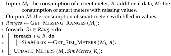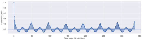
Figure 3. Auto-correlation plot of Energy Consumption.

Algorithm 4: Distance for additional information.

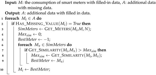Algorithm 5: Clustering for additional information.

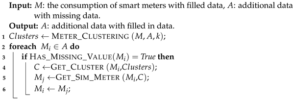3.2. Feature Engineering

This essential step allows the selection of the independent features to build a robust model. We choose a smart meter with the lowest number of missing values to conduct this study. For example, the smart meter $\#3003$ has only 192 missing values (which represents $1.09$ % of the $17,521$). We can identify the importance of some temporal features through the extensive visualization study of the consumption dataset that we carried out. According to Figure 4, we observe that energy consumption is variable during the different hours of the day. Thus, we identify the feature hour.

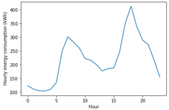
Figure 4. Hourly energy consumption by day.

Another feature is also depicted, which is based on Figure 2, previously presented. The average monthly energy consumption is not the same for all months of the year, which leads us to create a month feature. We then visualized energy consumption across different days of the week. As shown in Figure 5, the energy consumption also depends on the different days of the week. So, we decided to introduce the day_of_week feature.

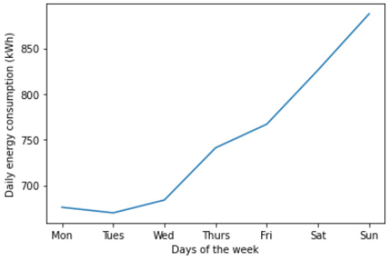
Figure 5. Average daily energy consumption by week.

When going through analyzing the behavior of energy consumption during the different days of the year based on Figure 6, the feature day_of_year is also added to our model.

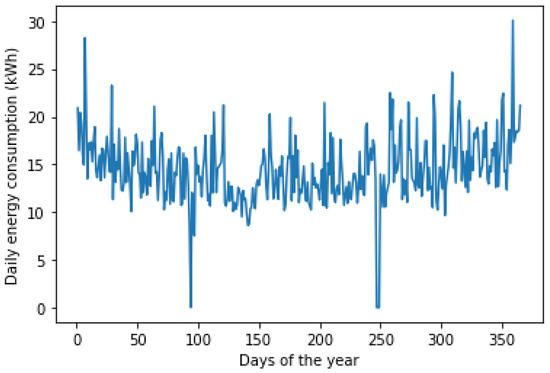
Figure 6. Average daily energy consumption by year.

The week_of_year is also considered an important feature in our analysis, as shown in Figure 7.

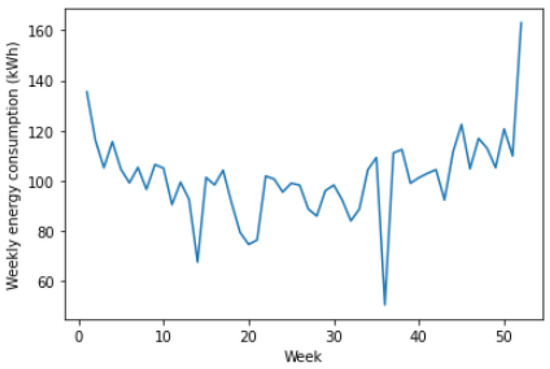
Figure 7. Average weekly energy consumption by year.

Besides temporal features, we depict some other additional features. In the exploratory data analysis step, we already defined the season feature. Then, we plotted the distribution of energy consumption for a given month of each season, categorized into weekdays and weekends. According to Figure 8, we observed that energy consumption was significantly higher during the weekends by contrast to weekdays. To leverage this pattern, we created a feature on whether the day being predicted for was a weekend called is_weekend.

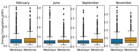
Figure 8. Distribution of energy consumption based on type of day (1 month from each season).

Paying close attention to the weather dataset, we distinguish a few missing values that may result from a sensor failure. The random sampling technique is then appropriate to fill missing values. After that, we apply the k-means algorithm on temperature data to identify the weather_cluster feature. As illustrated by Figure 9, the number of clusters is equal to 4. We also add the is_cold feature, which reflects the high energy consumption, especially in season 1.

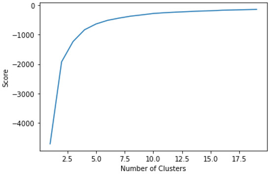
Figure 9. Elbow curve.

According to Figure 10, on weekdays, energy consumption sharply drops off at 7 am and picks up after 5 pm, most likely the standard working hours. As such, we took the liberty to introduce work_time (between 7 am and 5 pm on weekdays). Based on the same plot, we point out that energy consumption, both on weekdays and weekends, is higher between 5 pm and 8 pm. This pattern will be captured by the is_peak feature. We also add the dwelling type feature and the num_bedrooms from the additional information file as features (the most filled features).

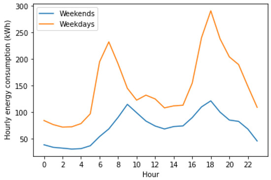
Figure 10. Average daily energy consumption (weekends and weekdays).

3.3. Training the Model

Needless to say, LSTM-based RNNs are an attractive choice for modeling sequential data like time series, as they incorporate contextual information from past inputs. Especially, the LSTM technique for time series forecasting has gained popularity because of its end-to-end modeling, learning complex non-linear patterns, and automatic feature extraction abilities. In this trend, we relied on a similar structure, and we start in the remainder presenting on the key embedding step.

Embedding

We adopt the Time2Vec proposed in [24] as our model’s embedding representation of time and weather features. The latter captures the main three properties (periodicity, invariance to time rescaling, and simplicity). For a given scalar notion of time t and weather w, Time2Vec of t and Weather2Vec of w, denoted as $x2v\left(x\right)$, are vectors of size $k+1$ defined as follows:

$$x2v\left(x\right)\left[i\right]=\left\{\begin{array}{cc}{w}_{i}x+{\phi }_i,\hfill & \mathrm{if}i=0\hfill \\ ϝ(w_{i}x+{\phi }_i),\hfill & \mathrm{if}1\le i\le k,\hfill \end{array}\right.$$

(1)

where $ϝ$ is a periodic activation function, and $w_i$ and ${\phi }_i$ are the learnable parameters. A vector representation for x allows it to be simply consumed by many architectures. In our implementation, we used $ϝ$ as the sine function.

3.4. Prediction & Explainability

In the following, we start by thoroughly presenting the building of the prediction model.

3.4.1. Prediction

In this paper, we introduce an explainable energy consumption prediction framework called Expect. Indeed, the latter tackles the problem as a daily, weekly, and monthly consumption regression task. We trained the prediction model on a historical 30-min intervals time-series from January to December 2017 besides weather information and several additional features. As depicted by Figure 1, the Expect prediction model operates as follows: after the pre-processing of the collected data (feature engineering step), both consumption and weather information are fed into the embedding proposed layers in order to extract the temporal and environmental hidden features. Therefore, these embedding results concatenated with additional information are fed afterwards to the model training step. Indeed, the success of LSTM-based neural networks with time-series data is owed to their ability to capture the long-term temporal dependencies. Therefore, for the model training step, we have to adopt the long short-term memory neural network model with the sequence-to-one architecture. Long-short term memory networks (LSTMs) are a type of RNN architecture that can learn long-term dependencies, utilizing the notion of memory. They were initially proposed by [25] and have since been varied and promoted in a wide range of publications to solve a wide range of issues. Commonly known as the forward pass LSTM network, it comprises three gates. For the cell’s state update $C_t$, a forget gate f and an input gate I are created. An output gate o determines how much information about the current input $x_t$ should be stored in the current output cell $h_t$. The gates’ functionalities are computed as follows:

$$f_t=\sigma (W_f.[h_{t-1},x_t]+b_f)$$

(2)

$$i_t=\sigma (W_i.[h_{t-1},x_t]+b_i)$$

(3)

$${\widehat{C}}_t=tanh(W_c.[h_{t-1},x_t]+b_c)$$

(4)

$$C_t=f_t\times C_{t-1}+i_t\times {\widehat{C}}_t$$

(5)

$$o_t=\sigma (W_o.[h_{t-1},x_t]+b_o)$$

(6)

$$h_t=o_t\times tanh\left(C_t\right).$$

(7)

We carried out our experiments under a computer environment with Ubuntu 18.04.3 LTS (CPU: Intel Xeon Processor (Skylake) × 8, RAM: $16\mathrm{Gb}$), with a 3.7 Python version and a 2.3.1 Keras version. We experiment with different architectures with varying numbers of hidden LSTM units to fine-tune parameters for the prediction process for the three different tasks (daily, weekly, and monthly). Finally, we designed the final parameter setups of the prediction model as shown in Table 3.

Table 3. The proposed Expect prediction model architecture.

Type	Daily	Weekly	Monthly
Embedding dimension	48	48	48
Sequences size	48	48	48
LSTM layers	1	1	2
LSTM units	100	200	200, 100
Epochs	50	100	200
Optimizer/Loss	Adam/MSE	Adam/MSE	Adam/MSE

3.4.2. Explainability

This phase presents an explainable module to understand why our predictive model makes energy consumption forecasts. In the literature, they have proposed many methods and frameworks because of the inherent explainability of a predictive model like LIME [26] or SHAPE [27]. It is worthy of mention that the existing well-known frameworks are designed for several “homogeneous” types of data tabular, text, and images. Nevertheless, our built prediction model is based on “heterogeneous” embedded and tabular data. In doing so, we have a flip of the coin for high achieved accuracy, since the existing frameworks do not apply to our built predictive model. Thence, we rely on an agnostic method to explain our black-box model in this remainder. We based the proposed method mainly on the Partial Dependence Plots [23], which show the effect that a feature would have on the predictions of the model. This partial dependence function shows the relationship between a feature and the predicted outcome. Besides, this dependence function can be explained to the user as the varying of a specific feature influencing the model’s forecasting. We change a given “selected” feature and leave the other features unchanged. Thence, we ask the built model what would happen to the energy consumption, that is, our target variable.

We opted for PDP to underscore the marginal effect one or two features can have on the predicted outcome of a predictive model [23]. In doing so, we can unveil the type of relationship between the target and a feature that is linear, monotonic, or even more complex.

$${\widehat{f}}_{x_S}\left(x_S\right)=E_{x_C}\left[\widehat{f}(x_S,x_C)\right]=\int \widehat{f}(x_S,x_C)d\mathbb{P}\left(x_C\right),$$

(8)

where $x_S$ stands for the set are the target features, that is, those for which the partial dependence function is plotted since we know their effect on the prediction, whereas $x_C$ stands for the set of the other features fed to the predictive model $\widehat{f}$. The feature vectors $x_S$ and $x_C$ combined make up the total feature space x. Partial dependence works by marginalizing the predictive model output over the distribution of the features in the set C. Thus, the plot function glances at the relationship between the sought-after set S features and the predicted outcome.

Through the Algorithm 6, we describe how the PDP of a given feature is computed.

Algorithm 6: Computing the PDP values.

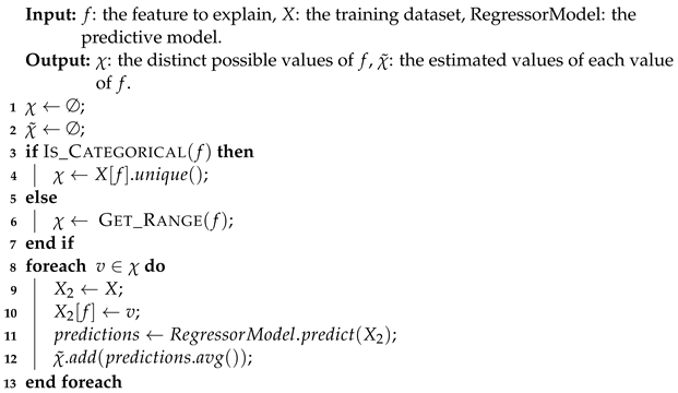As clearly underscored by its pseudo-code, the latter uses the training dataset X and the predictive model $RegressorModel$. Thence, it starts by checking whether the feature f is categorical or continuous through the Is_Categorical function (line 3). Then, it computes all its possible values $\chi$ (lines 4–6). If we are dealing with a categorical feature, $\chi$ is filled with the unique values of f (line 4). With a continuous feature, we get the $min\left(\right)$ and $max\left(\right)$ values of the feature f through the Get_Range function (line 6). After that, for each possible value (v) of $\chi$, the algorithm creates a new dataset $X_2$ by replacing the feature value with v and makes predictions on the new training dataset (line 11). Finally, the algorithm computes the average of the predictive values, which is added to the estimated value $\tilde{\chi }$ (line 12). Besides, the proposed explainable approach is rather global; to wit, it explains the behavior of the predictive model based on Partial Dependence Plots (PDP) of the extracted features (Section 3.2). Thus, whenever a user has a predictive value, it can project the input values to the PDP to explain why he had this predictive value.

4. Experimental Results

In this section, we present our experimental results, using a real-world energy consumption dataset for the performance assessment of the proposed Expect approach versus the competing baseline methods. Besides, we pay close attention to the interpretability of the obtained results using the PDP-based approach.

4.1. Evaluation Metrics

The prediction performance of our model and the baseline models are evaluated using the mean squared error (MSE) and the mean absolute error (MAE), which are defined respectively in the following equations:

$$MSE=\frac{1}{n}\sum _{i=1}^n{(c_i-{\widehat{c}}_i)}^2$$

(9)

$$MAE=\frac{1}{n}\sum _{i=1}^n|c_i-{\widehat{c}}_i|,$$

(10)

where n stands for the size of the tested consumption observations, $c_i$ for the ground-truth consumption, and ${\widehat{c}}_i$ for the predicted consumption yield by the model of the ith observation. MSE (Equation (9)) and MAE (Equation (10)) are the most used metrics to assess the average error between forecast and actual values.

4.2. Results and Discussion

To accurately test our proposed Expect approach, we led a comparison with the existing consumption prediction baseline methods; the statistical linear regression model proposed in [5] and the machine learning-based Random forest model implemented in [16]. In addition, for the sake of a fair comparison, we tested all the baseline methods using the same datasets. We evaluate the different approaches using the random sampling-based data completion (RDC) to assess the impact of using the seasonality-based data completion (SDC) Algorithm 2. In addition, the additional data missing values are filled in using distance-based data completion (DDC), and clustering-based data (CDC) completion approach described respectively by Algorithms 4 and 5. Therefore, we have got four different datasets for the final evaluation. Table 4, Table 5, Table 6 and Table 7 glance at the obtained values for both MAE and MSE metrics by the Expect approach versus its competitors. We analyze the models’ performance under three different prediction tasks daily, weekly, and monthly, representing a different degree of efficiency in the long term. In terms of MAE values, Expect outperforms all baseline methods using the SDC with DDC and SDC with CDC datasets for the three different prediction tasks. Although on both RDC with DDC and RDC with CDC the performances of the proposed method are slightly worse than the performances of the Random forest model for the monthly task, it still outperforms all other baselines. Through the experimental process results, the different approaches give varied MSE values. For both SDC with DDC and SDC with CDC datasets, our Expect approach, both daily and weekly prediction tasks’ values are reduced to ($33.67$, $408.61$) and ($33.63$, $408.61$), respectively, with an improvement of ($65.32\%$, $187.91\%$) and ($65.73\%$, $189.29\%$) according to the best performing baseline. For the two RDC datasets, our Expect flagged better results for only the weekly task. Nevertheless, it is slightly outperformed by the baselines for the remaining two tasks. Further analyses can extract different information in Table 8, the seasonality-based data completion method proves its efficiency to improve the performance of prediction models. The comparative analysis of the resulting table shows that our approach is effective with both daily and weekly tasks but is less accurate in the long-term prediction task (monthly). The size of the used dataset can explain it (one year), in which we do not exploit and extract complex patterns for each specific month. Nevertheless, using Random sampling for data completion achieves a better performance for the monthly task.

Table 4. Performance evaluation with RDC and DDC.

Method	Resolution	MSE	MAE
Linear Regression	Daily	49.85	4.86
	Weekly	1157.22	23.77
	Monthly	14,174	79.99
Random Forest	Daily	48.68	4.78
	Weekly	1130.06	23.31
	Monthly	13,818.84	78.40
Expect	Daily	60.01	4.28
	Weekly	566.91	13.82
	Monthly	29,521.40	121.16

Table 5. Performance evaluation with RDC and CDC.

Method	Resolution	MSE	MAE
Linear Regression	Daily	58.00	5.1738
	Weekly	1992.93	30.46
	Monthly	14,233.43	81.31
Random Forest	Daily	56.66	5.0797
	Weekly	1945.24	29.89
	Monthly	13,674.78	78.87
Expect	Daily	59.98	4.28
	Weekly	565.86	13.80
	Monthly	29,516.15	121.16

Table 6. Performance evaluation with SDC and DDC.

Method	Resolution	MSE	MAE
Linear Regression	Daily	51.54	4.98
	Weekly	2174.49	32.31
	Monthly	35,861.35	131.02
Random Forest	Daily	57.52	5.09
	Weekly	2257.00	31.95
	Monthly	37,614.87	132.55
Expect	Daily	33.67	3.29
	Weekly	408.61	11.37
	Monthly	36,266.74	127.98

Table 7. Performance evaluation with SDC and CDC.

Method	Resolution	MSE	MAE
Linear Regression	Daily	51.65	5.02
	Weekly	2182.02	32.68
	Monthly	36,124.15	134.02
Random Forest	Daily	51.16	4.94
	Weekly	2158.74	32.14
	Monthly	35,617.61	132.07
Expect	Daily	33.63	3.29
	Weekly	408.61	11.36
	Monthly	36,278.63	128.03

Table 8. Performance of the Expect framework using the different data completion methods.

Data Completion	MSE			MAE
	Daily	Weekly	Monthly	Daily	Weekly	Monthly
RDC and DDC	60.01	566.91	29,521.40	4.28	13.82	121.16
RDC and CDC	59.98	565.86	29,516.15	4.28	13.80	121.16
SDC and DDC	33.67	408.61	36,266.74	3.29	11.37	127.98
SDC and CDC	33.63	408.61	36,278.63	3.29	11.36	128.03

4.3. Explaining the Prediction

After building and testing our predictive model, users can use this model and thence predict the energy consumption in the future according to current data number of bedrooms, temperature, dwelling type, to name but a few. Besides, even highly accurate the built model is not, sadly, interpretable that can affect in trust faced by the users. Because the built model can make only predictions with no explanations to justify the predictive value. Several machine learning algorithms are “inherently” interpretable, for example, decision trees and random forests, which can provide the prediction with useful rules that are used to make these predictions, and other algorithms (like the proposed by us) are black-box models that make only predictions. Therefore, we have proposed on top of our predictive model an explainable layer that can explain to users why the predicted model gives such energy consumption. The proposed explainable layer is based on graphic interpretation by the user. In doing so, we relied on the PDP to unveil what happens to energy consumption whenever a feature changes while keeping all other features constant. The obtained values, that is, the predictions and possible values of each categorical and continuous feature, are projected into plots. In the remainder, we try to present some plots generated by our explainable layer and the built predictive model.

Figure 11 shows a pretty clear interpretation. It sketches an important impact of dwelling type features on energy consumption. Indeed, whenever we vary the dwelling type, the energy consumption also varies. In the same trend, we can explain a high consumption dwelling type is 1 or 2, which represents, respectively, a semi-detached house and a terraced house. A closer look at Figure 12 puts forward the considerable impact of the number of bedrooms’ feature on energy consumption. Indeed, we can notice a reciprocal connection between energy consumption and the number of bedrooms.

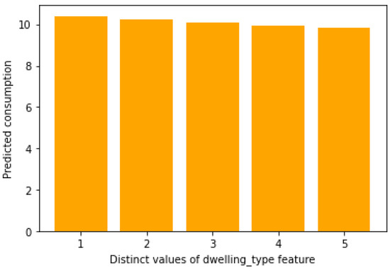
Figure 11. Impact of the dwelling type on the energy consumption.

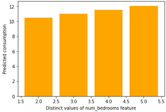
Figure 12. Impact of the number of bedrooms on the energy consumption.

Figure 13 also shows the impact of the temperature on energy consumption. Thus, as soon as the temperature curve shows that whenever the temperature increases, the energy consumption decreases.

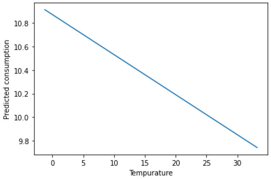
Figure 13. Impact of the temperature on the energy consumption.

The above-given figures glance at the behavior of some features for the outcome of the predictive model. Thus, we can notice a positive correlation between these features and the target variable. Using these figures, users can position themselves to justify the predictive energy consumption. In other words, in the case of high consumption, a user can check whether there is a high number of bedrooms and/or if the dwelling type is 4 or 5.

5. Conclusions and Future Work

In this paper, we introduced the Expect framework, which has shown very encouraging and self-explaining daily, weekly and monthly predictions for the electricity consumption of customers. We relied on an LSTM-based neural network model that ingested consumption data as well as external information, such as weather condition, dwelling type, and so forth.

Expect has shown evidence of resilience to the missing values, and we especially dealt with a vast number of missing values. In terms of accuracy, Expect has been shown to provide very encouraging results, versus its competitors, especially for the daily and weekly consumption forecasting.

The obtained results in this paper open up many perspectives. In the following, we present some promising future research paths from which we cite:

• Incremental learning of the predictive model: The steady ingestion of the low data on energy consumption sent out by smart meters is heading us towards the proposal of new incremental predictions that, in lieu of departing from scratch, will seed the already existing model;
• New explainability model for heterogeneous model: The predictive model that we developed has unveiled a compelling new framework, that, unlike the existing ones, would be able to work alongside our efficient prediction model. The new explainability framework would address global and local explainabilty views. In addition, we plan to improve this part of the proposed framework; now the user can interpret the provided graphic to explain why it would have such a prediction, that is, extract automatically predictive rules that can explain the provided prediction;
• Development of a personalized “trustworthy” virtual coach for energy consumption: The latter’s aim is to engage customers with personalized, actionable advice to improve their consumption and increase their satisfaction. This virtual coach aims to provide tailored advice, alerts and recommendations by learning every household consumption behavior.

References

- Kumar, A.; Shankar, R.; Aljohani, N.R. A big data driven framework for demand-driven forecasting with effects of marketing-mix variables. Ind. Mark. Manag. 2020, 90, 493–507. [Google Scholar] [CrossRef]
- Sezer, O.B.; Gudelek, M.U.; Ozbayoglu, A.M. Financial time series forecasting with deep learning: A systematic literature review: 2005–2019. Appl. Soft Comput. 2020, 90, 106181. [Google Scholar] [CrossRef] [Green Version]
- Deb, C.; Zhang, F.; Yang, J.; Lee, S.E.; Shah, K.W. A review on time series forecasting techniques for building energy consumption. Renew. Sustain. Energy Rev. 2017, 74, 902–924. [Google Scholar] [CrossRef]
- Chujai, P.; Kerdprasop, N.; Kerdprasop, K. Time Series Analysis of Household Electric Consumption with ARIMA and ARMA Models. In Proceedings of the International MultiConference of Engineers and Computer Scientists, IMECS 2013, Hong Kong, China, 13–15 March 2013; Volume I. [Google Scholar]
- Fumo, N.; Rafe Biswas, M. Regression analysis for prediction of residential energy consumption. Renew. Sustain. Energy Rev. 2015, 47, 332–343. [Google Scholar] [CrossRef]
- Beccali, M.; Ciulla, G.; Lo Brano, V.; Galatioto, A.; Bonomolo, M. Artificial neural network decision support tool for assessment of the energy performance and the refurbishment actions for the non-residential building stock in Southern Italy. Energy 2017, 137, 1201–1218. [Google Scholar] [CrossRef]
- Kong, W.; Dong, Z.Y.; Jia, Y.; Hill, D.J.; Xu, Y.; Zhang, Y. Short-Term Residential Load Forecasting Based on LSTM Recurrent Neural Network. IEEE Trans. Smart Grid 2019, 10, 841–851. [Google Scholar] [CrossRef]
- Zhong, H.; Wang, J.; Jia, H.; Mu, Y.; Lv, S. Vector field-based support vector regression for building energy consumption prediction. Appl. Energy 2019, 242, 403–414. [Google Scholar] [CrossRef]
- Abbasi, R.A.; Javaid, N.; Ghuman, M.N.J.; Khan, Z.A.; Ur Rehman, S.; Amanullah. Short Term Load Forecasting Using XGBoost. In Web, Artificial Intelligence and Network Applications; Barolli, L., Takizawa, M., Xhafa, F., Enokido, T., Eds.; Springer International Publishing: Cham, Switzerland, 2019; pp. 1120–1131. [Google Scholar]
- Kim, J.Y.; Cho, S.B. Electric Energy Consumption Prediction by Deep Learning with State Explainable Autoencoder. Energies 2019, 12, 739. [Google Scholar] [CrossRef] [Green Version]
- Khandelwal, I.; Adhikari, R.; Verma, G. Time Series Forecasting Using Hybrid ARIMA and ANN Models Based on DWT Decomposition. Procedia Comput. Sci. 2015, 48, 173–179. [Google Scholar] [CrossRef] [Green Version]
- Kim, T.Y.; Cho, S.B. Predicting residential energy consumption using CNN-LSTM neural networks. Energy 2019, 182, 72–81. [Google Scholar] [CrossRef]
- Jallal, M.A.; González-Vidal, A.; Skarmeta, A.F.; Chabaa, S.; Zeroual, A. A hybrid neuro-fuzzy inference system-based algorithm for time series forecasting applied to energy consumption prediction. Appl. Energy 2020, 268, 114977. [Google Scholar] [CrossRef]
- Kao, Y.S.; Nawata, K.; Huang, C.Y. Predicting Primary Energy Consumption Using Hybrid ARIMA and GA-SVR Based on EEMD Decomposition. Mathematics 2020, 8, 1722. [Google Scholar] [CrossRef]
- Yucong, W.; Bo, W. Research on EA-Xgboost Hybrid Model for Building Energy Prediction. J. Phys. Conf. Ser. 2020, 1518, 012082. [Google Scholar] [CrossRef]
- Ilic, I.; Görgülü, B.; Cevik, M.; Baydogan, M.G. Explainable boosted linear regression for time series forecasting. Pattern Recognit. 2021, 120, 108144. [Google Scholar] [CrossRef]
- Zhang, B.; Zhao, C. Dynamic turning force prediction and feature parameters extraction of machine tool based on ARMA and HHT. Proc. Inst. Mech. Eng. Part C J. Mech. Eng. Sci. 2020, 234, 1044–1056. [Google Scholar] [CrossRef]
- Mehedintu, A.; Sterpu, M.; Soava, G. Estimation and Forecasts for the Share of Renewable Energy Consumption in Final Energy Consumption by 2020 in the European Union. Sustainability 2018, 10, 1515. [Google Scholar] [CrossRef] [Green Version]
- Aslam, S.; Herodotou, H.; Mohsin, S.M.; Javaid, N.; Ashraf, N.; Aslam, S. A survey on deep learning methods for power load and renewable energy forecasting in smart microgrids. Renew. Sustain. Energy Rev. 2021, 144, 110992. [Google Scholar] [CrossRef]
- Alanbar, M.; Alfarraj, A.; Alghieth, M. Energy Consumption Prediction Using Deep Learning Technique. Int. J. Interact. Mob. Technol. 2020, 14, 166–177. [Google Scholar] [CrossRef]
- Debnath, K.B.; Mourshed, M. Forecasting methods in energy planning models. Renew. Sustain. Energy Rev. 2018, 88, 297–325. [Google Scholar] [CrossRef] [Green Version]
- Triguero, I. FUZZ-IEEE Competition on Explainable Energy Prediction. 2020. Available online: https://ieee-dataport.org/competitions/fuzz-ieee-competition-explainable-energy-prediction (accessed on 17 November 2021).
- Friedman, J.H. Greedy function approximation: A gradient boosting machine. Ann. Stat. 2001, 29, 1189–1232. [Google Scholar] [CrossRef]
- Kazemi, S.M.; Goel, R.; Eghbali, S.; Ramanan, J.; Sahota, J.; Thakur, S.; Wu, S.; Smyth, C.; Poupart, P.; Brubaker, M. Time2Vec: Learning a Vector Representation of Time. arXiv 2019, arXiv:1907.05321. [Google Scholar]
- Hochreiter, S.; Schmidhuber, J. Long Short-Term Memory. Neural Comput. 1997, 9, 1735–1780. [Google Scholar] [CrossRef] [PubMed]
- Ribeiro, M.T.; Singh, S.; Guestrin, C. “Why Should I Trust You?”: Explaining the Predictions of Any Classifier. arXiv 2016, arXiv:1602. [Google Scholar]
- Lundberg, S.; Lee, S.I. A unified approach to interpreting model predictions. arXiv 2017, arXiv:1705.07874. [Google Scholar]
Publisher’s Note: MDPI stays neutral with regard to jurisdictional claims in published maps and institutional affiliations. |
© 2022 by the authors. Licensee MDPI, Basel, Switzerland. This article is an open access article distributed under the terms and conditions of the Creative Commons Attribution (CC BY) license (https://creativecommons.org/licenses/by/4.0/).