Some Results on Measures of Interaction among Risks

Abstract

It has become a common understanding that financial risk can spread rapidly from one institution to another, and the stressful status of one institution may finally result in a systemic crisis. One popular method to assess and quantify the risk of contagion is employing the co-risk measures and risk contribution measures. It is interesting and important to understand how the underlining dependence structure and magnitude of random risks jointly affect systemic risk measures. In this paper, we mainly focus on the conditional value-at-risk, conditional expected shortfall, the delta conditional value-at-risk, and the delta conditional expected shortfall. Existing studies mainly focus on the situation with two random risks, and this paper makes some contributions by considering the scenario with possibly more than two random risks. By employing the tools of stochastic order, positive dependence concepts and arrangement monotonicity, several results concerning the usual stochastic order, increasing convex order, dispersive order and excess wealth order are presented. Concisely speaking, it is found that for a large enough stress level, a larger random risk tends to lead to a more severe systemic risk. We also performed some Monte Carlo experiments as illustrations for the theoretical findings.

1. Introduction

Researchers’ interest in risk contagion or systemic risk has been rising gradually since the financial crisis in 2007–2009. The so-called contagion risk refers to the fact that when one or more components of the portfolio collapse, it will lead to the collapse of other components, thus making the entire portfolio at risk. Many scholars pay attention to the interaction of risks. For example, the essay of [1] proposed an $\mathrm{LPPL}$ model for market bubbles or collapse, which aims to diagnose and describe the relationship between future market prices and prices of IIGPS countries. Yang et al. in [2] focused on correlation change and risk spillovers of the Chinese mainland and the London stock markets, using $\mathrm{CoVaR}$ and $\mathrm{CoES}$ as two risk measures. Meanwhile, the paper by [3] measured the risk spillover effect among carbon markets of some countries in China through the regular vine copula using the $\mathrm{CoES}$ approach. In many recent studies regarding the risk of contagion, the focus is put on conditional risk distributions instead of unconditional ones. Therefore, relevant scholars have adjusted the risk measures commonly used in the financial industry to include the impact of the interaction.

Recall that, given a risk X with distribution function F, its Value-at-Risk ($\mathrm{VaR}$) at level p (or the pth-quantile) is defined as ${\mathrm{VaR}}_p\left(X\right)=F^{-1}\left(p\right)=inf\{x:F\left(x\right)\ge p\}$, for $p\in (0,1)$. In 1994, the J.P. Morgan investment bank first proposed to use the $\mathrm{VaR}$ as a measurement of financial risk. After that, the $\mathrm{VaR}$ measure was soon widely adopted by banks, and the Bank for International Settlements took it as the risk model for measuring capital adequacy in the first pillar of Basel II in 1995. $\mathrm{VaR}$ measures the tail loss under normal market fluctuations; that is, the extreme loss under normal market fluctuations. It explains the maximum possible loss under normal market fluctuations rather than the loss under extreme market conditions, such as war, politics and financial crisis. People gradually find that $\mathrm{VaR}$ itself has certain limitations. First, the $\mathrm{VaR}$ model itself can not accurately measure the future market risk because it uses historical data to predict future losses and usually assumes that the correlation between variables remains unchanged. However, in practice, the correlation changes and the pre-calculated results sometimes do not agree with reality. Second, the concept of $\mathrm{VaR}$ does not possess subadditivity. That is, the overall risk of a financial institution cannot be reduced by combining the risks of its subsidiaries, which brings great trouble to the risk measurement. However, subadditivity is very important in financial management and is one of the most important characteristics of risk measurement. For this reason, refs. [4,5,6] in 2001 proposed another market risk measure, the expected shortfall (ES), which is both subadditive and easy to use, and then [7,8,9] explored the application of $\mathrm{ES}$ further. As a successor of $\mathrm{VaR}$, $\mathrm{ES}$ is defined as ${\mathrm{ES}}_p\left(X\right)=E\left(X\right|X>{\mathrm{VaR}}_p\left(X\right))$. If the distribution function F is continuous, the following identity holds: for $p\in (0,1)$, ${\mathrm{ES}}_p\left(X\right)=\frac{1}{1-p}{\int }_p^1{\mathrm{VaR}}_t\left(X\right)\mathrm{d}t$. See [10,11] and references therein for comprehensive overviews of risk measures of univariate risks.

Both $\mathrm{VaR}$ and $\mathrm{ES}$ play a vital role in risk management since their emergence. However, in the past decade, people have begun to realize that the interaction among risks within a portfolio also plays an important role in determining the measure of risk. In recent years, the interaction between supervision and discussion of risks has been significantly strengthened in financial risk analysis. For example, [12,13,14] proved consistent results for the $\mathrm{VaR}$ and $\mathrm{ES}$ of aggregate risk. In this context, risk measures are utilized to evaluate marginal and aggregate risks and to assess the systemic risk since the recent global financial crisis. The past three decades have witnessed several financial crises, globally or regionally, and one important thing people learned from these crises is that financial institutions possess strong interaction, which affects institutions differently. The bankruptcy of some banks may lead to the bankruptcy of more banks, while some banks have very little effect on the whole financial market. That is to say, systemic risk should be measured more carefully and delicately.

The current financial system has various systemic risk measures, such as conditional Value-at-Risk ($\mathrm{CoVaR}$, for a formal definition, see (2)) introduced by [15,16], the conditional expected shortfall ($\mathrm{CoES}$, for a formal definition, see (3)) introduced by [3,17], the Targeted Sparse Systemic Risk Index by [18] and so on. Basically, the existing systemic risk measures fall into two classes: co-risk measures and risk contribution measures. Co-risk measures take the dependence structure among isolated risks into consideration. From the viewpoint of probability, these measures consider the conditional event that specific risks or the total risk are under pressure. Examples include $\mathrm{CoVaR}$ and $\mathrm{CoES}$. In parallel, risk contribution measures quantify how a stressful situation for an institution brings forth extra risk to another or even the whole portfolio. Examples of risk contribution measures can be found in [15,17,19,20].

To the best of our knowledge, the existing literature on co-risk measures and risk contribution measures mainly focus on paired risk. For example, [17] studied the dependence consistency that $\mathrm{CoVaR}$ showed when holding the marginal risks’ distributions, a more concordant dependence structure will result in a larger $\mathrm{CoVaR}$. Recently, ref. [21] extended this finding to other risk measures such as $\mathrm{CoES}$, $\mathsf{\Delta }\mathrm{CoVaR}$ and $\mathsf{\Delta }\mathrm{CoES}$ under some positive dependence structures; they also found a more concordant dependence structure will imply a larger $\mathrm{CoES}$, $\mathsf{\Delta }\mathrm{CoVaR}$ and $\mathsf{\Delta }\mathrm{CoES}$, respectively, when the marginal distribution possesses some specific stochastic orders. For paired risks, the stress event of one risk will have its own impact on another risk, and vice versa. In order to understand the risk level of paired risks, ref. [22] studied how the magnitude of two risks and the dependence structure between them affect the co-risk measurement and risk contribution measurements, such as using the popular $\mathrm{CoVaR}$, $\mathrm{CoES}$, $\mathsf{\Delta }\mathrm{CoVaR}$ and $\mathsf{\Delta }\mathrm{CoES}$. Usually, there are more than two institutions in a financial market, and interaction among institutions is more complicated. When considering the risk contagion behavior between two specific institutions, the impact from other institutions should not be ignored. However, to the best of our knowledge, the existing literature has not investigated the difference between risk contagion from one institution to another and that from the latter to the former when there are more than two institutions in the market. When there are possibly more than two risks, are the results of paired risk exploration in [22] are still applicable? Are there any general results?

Along the study of [22], this paper aims to further study how a marginal distribution of risks and dependence structure affects the overall condition risk measurement and risk contribution measurement in system risk when there are two or more risks interconnected with each other. The concept of copula and survival copula is employed to characterize the dependence structure among risks, combined with the arrangement monotonicity, exchangeability and some other dependence properties. For exchangeable survival copula, the stochastically larger marginal risk has a larger $\mathrm{CoVaR}$. For asymmetric survival copula possessing arrangement monotonicity, when the stress level is large enough, the stochastically larger marginal risk is proved to attain a larger $\mathrm{CoVaR}$. Similar phenomena can be observed for $\mathrm{CoES}$, $\mathsf{\Delta }\mathrm{CoVaR}$ and $\mathsf{\Delta }\mathrm{CoES}$, where the larger random risk, in the condition of increasing convex order, dispersive order and excess wealth order, tends to have a severe impact on the systemic risk. Our results show that when considering the risk contagion effect inside two institutions if the dependence structure among institutions in the whole market possesses some local property, such as symmetry of arrangement monotonicity, the comparing relationship between the two institutions is similar to that under the situation where the market only has two institutions.

The rest of the paper proceeds as follows: Section 2 reviews some related concepts and technical results concerning the detailed discussions in the sequel. Section 3 presents the comparison results of two co-risk measures, $\mathrm{CoVaR}$ and $\mathrm{CoES}$. The comparison results from the two risk contribution measures, $\mathsf{\Delta }\mathrm{CoVaR}$ and $\mathsf{\Delta }\mathrm{CoES}$, are developed in Section 4. Finally, several Monte Carlo experiments are carried out in Section 5 to illustrate the main findings.

2. Preliminaries

Throughout this paper, we denote $\mathit{p}=(p_1,\cdots ,p_n)\in {(0,1)}^n$. For $1\le i<j\le n$, we denote $\mathit{p}(i;\alpha )=(p_1,\cdots ,p_{i-1},\alpha ,p_{i+1},\cdots ,p_n)$ and

$$\mathit{p}(i,j;\alpha ,\beta )=(p_1,\cdots ,p_{i-1},\alpha ,p_{i+1},\cdots ,p_{j-1},\beta ,p_{j+1},\cdots ,p_n).$$

Let $\mathit{X}=(X_1,X_2,\cdots ,X_n)$ be a random vector, and ${\mathit{X}}_{-i}=(X_1,\cdots ,X_{i-1},X_{i+1},\cdots ,X_n)$ be a random vector obtained by deleting the ith argument from $\mathit{X}$.

2.1. Stochastic Orders

The following stochastic orders play a key role in this study.

Definition 1.

Let X and Y be two random variables with respective distribution functions $F_X$ and $F_Y$ and tail functions ${\overline{F}}_X=1-F_X$ and ${\overline{F}}_Y=1-F_Y$, respectively. Then, X is said to be smaller than Y,

(i) 

in the usual stochastic order (denoted by $X{\le }_{st}Y$) if $\overline{F}\left(t\right)\le \overline{G}\left(t\right)$ (or $F\left(t\right)\ge G\left(t\right)$) for all $t\in \mathbb{R}$;

(ii) 

in the increasing convex order (denoted by $X{\le }_{\mathrm{icx}}Y$) if ${\int }_t^{\infty }{\overline{F}}_X\left(x\right)\mathrm{d}x\le {\int }_t^{\infty }{\overline{F}}_Y\left(x\right)\mathrm{d}x$, for all $t\in \mathbb{R}$;

(iii) 

in the dispersive order (denoted by $X{\le }_{disp}Y$) if $F_X^{-1}\left(p\right)-F_X^{-1}\left(q\right)\le F_Y^{-1}\left(p\right)-F_Y^{-1}\left(q\right)$ for all $0\le q<p<1$;

(iv) 

in the excess wealth order (denoted by $X{\le }_{ew}Y$) if ${\int }_{F_X^{-1}\left(p\right)}^{\infty }{\overline{F}}_X\left(x\right)\mathrm{d}x\le {\int }_{F_Y^{-1}\left(p\right)}^{\infty }{\overline{F}}_Y\left(x\right)\mathrm{d}x$, for all $p\in (0,1)$.

It is well-known that (see [23]) $X{\le }_{st}Y\Rightarrow X{\le }_{icx}Y$ and $X{\le }_{disp}Y\Rightarrow X{\le }_{ew}Y$, but not the converse. Stochastic orders are widely used in the study of finance, actuarial sciences, reliability theory and operation research, etc. For more on the properties and applications of stochastic orders, readers can refer to monographs [24,25,26]. The following lemma will be used to derive some main results.

Theorem 1

(Theorem 2.1 of [27]). For two random variables X and Y, $X{\le }_{icx}Y$ if and only if

$${\int }_0^1{F}_X^{-1}\left(t\right)\mathrm{d}\Phi \left(t\right)\le {\int }_0^1{F}_Y^{-1}\left(t\right)\mathrm{d}\Phi \left(t\right),$$

for any increasing convex function $\Phi :[0,1]\mapsto R.$

The notion of distortion function, popular in the recent study of actuarial and financial research, will also be utilized in deriving some of the main results. A distortion function h is a non-decreasing function mapping from $[0,1]$ to $[0,1]$ that satisfies $h\left(0\right)=0$ and $h\left(1\right)=1$. If h is continuous, the transformation of the tail function ${\overline{F}}_X=1-F_X$ of X given by ${\overline{F}}_h\left(x\right)=h\left({\overline{F}}_X\left(x\right)\right)=h\circ {\overline{F}}_X\left(x\right)$ defines a new tail function associated with a certain random variable $X_h$, which is said to be the h-distorted random variable induced from X. Readers who are interested in distortion functions can refer to [28,29]. The next lemma connects the dispersive order and distortion functions.

Lemma 1

(Lemma 14 of [21]). Let X and Y be two continuous random variables with distribution functions F and G, respectively. Let h be a concave distortion function and let g be another distortion function such that $h\left(t\right)\le g\left(t\right)$ for all $t\in [0,1]$. Denote by $X_h$ and $Y_g$ the distorted random variables induced, respectively, from X and Y, by the distortion functions h and g, respectively. If $X{\le }_{disp}Y$, then:

(i) 

$F_{X_h}^{-1}\left(p\right)-F_X^{-1}\left(p\right)\le F_{Y_g}^{-1}\left(p\right)-F_Y^{-1}\left(p\right)$, for all $p\in (0,1);$

(ii) 

$F_{X_g}^{-1}\left(p\right)-F_{X_h}^{-1}\left(p\right)\le F_{Y_g}^{-1}\left(p\right)-F_{Y_h}^{-1}\left(p\right)$, for all $p\in (0,1).$

2.2. Copula and Dependence

Copula is a useful tool for modeling the dependence structure among random risks.

Definition 2.

For $\mathit{X}=(X_1,\cdots ,X_n)$ with univariate marginal distribution functions $F_1,\cdots ,F_n$, and marginal survival functions ${\overline{F}}_1,\cdots ,{\overline{F}}_n$, if there exist some $C:{[0,1]}^n\mapsto [0,1]$ and $\widehat{C}:{[0,1]}^n\mapsto [0,1]$ such that the joint distribution function

$$F(x_1,\cdots ,x_n)=C(F_1\left(x_1\right),\cdots ,F_n\left(x_n\right)),$$

and the joint survival function

$$\overline{F}(x_1,\cdots ,x_n)=\widehat{C}({\overline{F}}_1\left(x_1\right),\cdots ,{\overline{F}}_n\left(x_n\right)),$$

for all $x_i$, $1\le i\le n$, then $C(u_1,\cdots ,u_n)$ and $\widehat{C}(u_1,\cdots ,u_n)$ are called the copula and survival copula of $\mathit{X}$, respectively.

For more on copulas, we refer readers to the comprehensive monograph [30]. Owing to the fact that random variable $\overline{F_i}\left(X_i\right)=1-F_i\left(X_i\right)$, $1\le i\le n$ are uniformly distributed over $[0,1]$, for $p_1,\cdots ,p_n\in (0,1)$. If the marginals are continuous, then the following inequality holds:

$$\widehat{C}(1-p_1,1-p_2,\cdots ,1-p_n)=\mathrm{P}(X_1>F_1^{-1}\left(p_1\right),X_2>F_2^{-1}\left(p_2\right),\cdots ,X_n>F_n^{-1}\left(p_n\right)).$$

For ease of reference, denote

$$\overline{C}(p_1,p_2,\cdots ,p_n)=\widehat{C}(1-p_1,1-p_2,\cdots ,1-p_n).$$

We will use some notions that formalize the idea of positive dependence of random vectors.

Definition 3.

For random vector $\mathit{X}$ and random variable Y,

(i) 

${\mathit{X}}_{-i}$ is said to be stochastically increasing (SI) in $X_i$ if the conditional distribution ${\mathit{X}}_{-i}|X_i=x_i$ is stochastically increasing as $x_i$ increases;

(ii) 

$\mathit{X}$ is said to be positive dependent through the stochastic order (PDS) if ${\mathit{X}}_{-i}{\uparrow }_{SI}{X}_i$ for $i=1,\cdots ,n$;

(iii) 

$\mathit{X}$ is said to be weakly stochastically increasing (WSI) in Y (denoted ${\mathit{X}\uparrow }_{WSI}Y$) if $\mathrm{P}(X_1\ge x_1,\cdots ,X_n>x_n\mid Y=y$) is increasing in y for all $x_1,\cdots ,x_n\in \mathbb{R}$;

(iv) 

$\mathit{X}$ is said to be positively dependent through the upper orthant (PDUO) if ${\mathit{X}}_{-i}{\uparrow }_{WSI}{X}_i$ for all $i=1,\cdots ,n$.

The following characterization will be utilized to derive some results in the sequel. According to [31], if the random vector $\mathit{X}$ has an absolutely continuous survival copula $\widehat{C}$, then given $i=1,\cdots ,n$, ${\mathit{X}}_{-i}{\uparrow }_{WSI}{X}_i$ is equivalent to

$$\frac{{\partial }^2\widehat{C}(p_1,\cdots ,p_n)}{{\partial p_i}^2}\le 0,$$

(1)

for any $p_i\in (0,1)$, namely, $\widehat{C}$ is concave in $u_i$.

It is well-known that SI, PDS, WSI and PDUO are all notions describing positive dependence among random variables. It is clear that for two random variables X and Y, ${X\uparrow }_{SI}Y$ is equivalent to ${X\uparrow }_{WSI}Y$, and a bivariate random vector $(X,Y)$ is PDUO if and only if it is PDS.

2.3. Co-Risk Measures

The systemic risk measure is usually utilized to quantify a financial institution’s contribution to the risk of other financial institutions or even the entire financial system. Co-risk measures are risk-adjusted versions of measures usually employed to assess isolated risks. In the past decade, co-risk measures and risk contribution measures have been increasingly used in actuarial portfolio analysis to evaluate systemic risk. One may refer to [16,17,32] and the references therein for further applications regarding co-risk measures.

Definition 4.

For a random vector $\mathit{X}$,

(i) 

the $\mathrm{CoVaR}$ of $X_i$ at stress level $p_i$ given that $X_j$ is under stress at level $p_j$ for $1\le j\ne i\le n$ is

$${\mathrm{CoVaR}}_{\mathit{p}}(X_i|{\mathit{X}}_{-i})={\mathrm{VaR}}_{p_i}\left(X_i|\bigcap _{1\le j\ne i\le n}\{X_j\ge {\mathrm{VaR}}_{p_j}\left(X_j\right)\}\right).$$

(2)

(ii) 

the $\mathrm{CoES}$ of $X_i$ at stress level $p_i$ given that $X_j$ is under stress at level $p_j$ for $1\le j\ne i\le n$ is

$${\mathrm{CoES}}_{\mathit{p}}(X_i|{\mathit{X}}_{-i})=\frac{1}{1-p_i}{\int }_{p_i}^1{\mathrm{CoVaR}}_{\mathit{p}(i;t)}\left(X_i\right|{\mathit{X}}_{-i})\mathrm{d}t.$$

(3)

2.4. Risk Contribution Measures

Apart from the co-risk measures, risk contribution measures quantify how a stress situation for a component affects another one, even the overall financial system. For more details on risk contribution measures and their applications, one can refer to [17,21].

Definition 5.

For a random vector $\mathit{X}$,

(i) 

$\mathsf{\Delta }\mathrm{CoVaR}$ of $X_i$ at stress level $p_i$ given that $X_j$ is under stress at level $p_j$ for $1\le j\ne i\le n$ is

$$\mathsf{\Delta }{\mathrm{CoVaR}}_{\mathit{p}}\left(X_i\right|{\mathit{X}}_{-i})={\mathrm{CoVaR}}_{\mathit{p}}\left(X_i\right|{\mathit{X}}_{-i})-{\mathrm{VaR}}_{p_i}\left(X_i\right)$$

(4)

(ii) 

$\mathsf{\Delta }\mathrm{CoES}$ of $X_i$ at stress level $p_i$ given that $X_j$ is under stress at level $p_j$ for $1\le j\ne i\le n$ is

$$\mathsf{\Delta }{\mathrm{CoES}}_{\mathit{p}}\left(X_i\right|{\mathit{X}}_{-i})={\mathrm{CoES}}_{\mathit{p}}\left(X_i\right|{\mathit{X}}_{-i})-{\mathrm{ES}}_{p_i}\left(X_i\right).$$

(5)

The next lemma for $\mathrm{CoVaR}$ is useful for deriving the main results in the sequel.

Lemma 2.

For a random vector $\mathit{X}=(X_1,X_2,\cdots ,X_n)$ having continuous marginal distributions $F_i$ for all $i=1,\cdots ,n$ and copula $C(u_1,\cdots ,u_n)$, which is the distribution function of $(U_1,\cdots ,U_n)$, then

$${\mathrm{CoVaR}}_{\mathit{p}}\left(X_i\right|{\mathit{X}}_{-i})=F_{X_i}^{-1}\left(F_{U_i\mid {\bigcap }_{1\le j\ne i\le n}\{U_j\ge p_j\}}^{-1}\left(p_i\right)\right),$$

(6)

and

$$F_{U_i\mid {\bigcap }_{1\le j\ne i\le n}\{U_j\ge p_j\}}\left(p_i\right)=1-\frac{\overline{C}(p_1,\cdots ,p_{i-1},p_i,p_{i+1},\cdots ,p_n)}{\overline{C}(p_1,\cdots ,p_{i-1},0,p_{i+1},\cdots ,p_n)}.$$

(7)

Proof. 

Since $(U_1,\cdots ,U_n)$ has the distribution function $C(u_1,\cdots ,u_n)$, which is the copula of $\mathit{X}$, one has for $p_i\in (0,1)$, $i=1,\cdots ,n$,

$$\begin{array}{ccc}& & 1-F_{X_i\mid {\bigcap }_{1\le j\ne i\le n}\{X_j\ge {\mathrm{VaR}}_{p_j}\left(X_j\right)\}}\left(x_i\right)\hfill \\ & =& \mathrm{P}(X_i\ge x_i\mid \bigcap _{1\le j\ne i\le n}\{X_j\ge {\mathrm{VaR}}_{p_j}\left(X_j\right)\})\hfill \\ & =& \mathrm{P}(F_{X_i}\left(X_i\right)\ge F_{X_i}\left(x_i\right)\mid \bigcap _{1\le j\ne i\le n}\{F_{X_j}\left(X_j\right)\ge p_j\})\hfill \\ & =& \frac{\mathrm{P}({\bigcap }_{1\le j\ne i\le n}\{F_{X_j}\left(X_j\right)\ge p_j\},F_{X_i}\left(X_i\right)\ge F_{X_i}\left(x_i\right))}{\mathrm{P}({\bigcap }_{1\le j\ne i\le n}\{F_{X_j}\left(X_j\right)\ge p_j\})}\hfill \\ & =& \frac{\overline{C}(p_1,\cdots ,p_{i-1},F_{X_i}\left(x_i\right),p_{i+1},\cdots ,p_n)}{\overline{C}(p_1,\cdots ,p_{i-1},0,p_{i+1},\cdots ,p_n)}\hfill \\ & =& \frac{\mathrm{P}(U_1\ge p_1,\cdots ,U_{i-1}\ge p_{i-1},U_i\ge F_{X_i}\left(x_i\right),U_{i+1}\ge p_{i+1},\cdots ,U_n\ge p_n)}{\mathrm{P}({\bigcap }_{1\le j\ne i\le n}{U}_j\ge p_j)}\hfill \\ & =& \mathrm{P}(U_i\ge F_{X_i}\left(x_i\right)\mid \bigcap _{1\le j\ne i\le n}\{U_j\ge p_j\})\hfill \\ & =& 1-F_{U_i\mid {\bigcap }_{1\le j\ne i\le n}\{U_j\ge p_j\}}(F_{X_i}\left(x_i\right)).\hfill \end{array}$$

Therefore, if

$$x_i=F_{X_i\mid {\bigcap }_{1\le j\ne i\le n}\{X_j\ge {\mathrm{VaR}}_{p_j}\left(X_j\right)\}}^{-1}\left(p_i\right),$$

one immediately has (6) and (7). □

In order to compare the degree of risk interaction of multivariate risks, given $\alpha \in (0,1)$, $\mathit{p}=(p_1,\cdots ,p_n)\in {(0,1)}^n$, for $\beta \in (0,1)$, denote $v_{\alpha }(\mathit{p},i,j;\beta )$ and ${\widehat{v}}_{\alpha }(\mathit{p},i,j;\beta )$ the solutions of equations

$$\beta =1-\frac{\overline{C}(p_1,\cdots ,p_{i-1},v_{\alpha }(\mathit{p},i,j;\beta ),p_{i+1},\cdots ,p_{j-1},\alpha ,p_{j+1},\cdots ,p_n)}{\overline{C}(p_1,\cdots ,p_{i-1},0,p_{i+1},\cdots ,p_{j-1},\alpha ,p_{j+1},\cdots ,p_n)},$$

and

$$\beta =1-\frac{\overline{C}(p_1,\cdots ,p_{i-1},\alpha ,p_{i+1},\cdots ,p_{j-1},{\widehat{v}}_{\alpha }(\mathit{p},i,j;\beta ),p_{j+1},\cdots ,p_n)}{\overline{C}(p_1,\cdots ,p_{i-1},\alpha ,p_{i+1},\cdots ,p_{j-1},0,p_{j+1},\cdots ,p_n)},$$

respectively.

2.5. Arrangement Monotonicity

Denote the permutation ${\tau }_{i,j}(x_1,\cdots ,x_i,\cdots ,x_j,\cdots ,x_n)=(x_1,\cdots ,x_j,\cdots ,x_i,\cdots ,x_n)$ for $1\le i<j\le n$. A real function $g\left(\mathit{x}\right):{\mathbb{R}}^n\mapsto \mathbb{R}$ is said to be arrangement increasing (AI) in $\{i,j\}$ such that $1\le i<j\le n$, if

$$(x_i-x_j)[g\left(\mathit{x}\right)-g\left({\tau }_{i,j}\left(\mathit{x}\right)\right)]\le 0\mathrm{for}\mathrm{any}{x}_i\le x_j.$$

(8)

Function g is said to be arrangement decreasing (AD) in $\{i,j\}$ such that $1\le i<j\le n$ if the inequality in (8) is reversed.

Arrangement monotone functions have been receiving more and more attention from researchers in risk management and operations research. Interested readers may refer to [33] for comprehensive properties on arrangement monotone functions.

At the end of this section, we finally recall one important lemma to be used in the sequel.

Lemma 3

(Lemma 4.7.1 in [34]). Suppose ${\int }_t^{\infty }\mathrm{d}\sigma \left(x\right)\ge 0$ for all t and one not necessarily positive measure $\sigma \left(x\right)$. Then,

$${\int }_{-\infty }^{+\infty }h\left(x\right)\mathrm{d}\sigma \left(x\right)\ge 0,$$

whenever the integrand $h\left(x\right)$ is nonnegative and increasing on the real line.

3. Co-Risk Measures

In this section, we discuss how the magnitude of marginal risks affects the corresponding $\mathrm{CoVaR}$ in a portfolio. It is of interest to compare the same co-risk measure incurred by risks of a different magnitude under the same stress levels. Specifically, we will propose several sufficient conditions for the following inequality.

$${\mathrm{CoVaR}}_{\mathit{p}(i,j;\alpha ,\beta )}\left(X_j\right|{\mathit{X}}_{-j})\ge {\mathrm{CoVaR}}_{\mathit{p}(i,j;\beta ,\alpha )}\left(X_i\right|{\mathit{X}}_{-i}).$$

(9)

That is, for ${\mathrm{CoVaR}}_{\mathit{p}(i,j;\alpha ,\beta )}\left(X_j\right|{\mathit{X}}_{-j})$, we consider the case when risk $X_{\ell }$ is under the stress level $p_{\ell }$ for $1\le \ell \le n$ and $\ell \ne i,j$, risk $X_j$ is under the stress level $\alpha$ and risk $X_i$ is under the stress level $\beta$. As for ${\mathrm{CoVaR}}_{\mathit{p}(i,j;\beta ,\alpha )}\left(X_i\right|{\mathit{X}}_{-i})$, we consider the case similar to the previous one by exchanging the two risks $X_i$ and $X_j$.

Theorem 2.

For the random vector $\mathit{X}$ with survival copula $\widehat{C}(u_1,\cdots ,u_n)$, $(u_1,\cdots ,u_n)\in {(0,1)}^n$,

(i) 

if $\widehat{C}(u_1,\cdots ,u_n)$ is symmetric, then $X_i{\le }_{st}{X}_j$ is equivalent to (9);

(ii) 

if $\widehat{C}(u_1,\cdots ,u_n)$ is AD in $1\le i<j\le n$, then $X_i{\le }_{st}{X}_j$ implies (9) for

$$\beta \ge 1-\frac{\overline{C}(p_1,\cdots ,p_{i-1},\alpha ,p_{i+1},\cdots ,p_{j-1},\alpha ,p_{j+1},\cdots ,p_n)}{\overline{C}(p_1,\cdots ,p_{i-1},0,p_{i+1},\cdots ,p_{j-1},\alpha ,p_{j+1},\cdots ,p_n)}.$$

Proof. 

Denote the random vector $(U_1,\cdots ,U_n)$ having survival function $\widehat{C}(1-u_1,\cdots ,1-u_n)$.

Case (i): Note that $X_i{\le }_{st}{X}_j$ is equivalent to

$$F_{X_i}^{-1}\left(p\right)\le F_{X_j}^{-1}\left(p\right)$$

(10)

for any $p\in (0,1)$. By the symmetry of $\widehat{C}$ and (7), one has

$$\begin{array}{ccc}& & F_{U_i|{\bigcap }_{\genfrac{}{}{0pt}{}{1\le k\le n,}{k\ne i,j}}\{U_k\ge p_k\},U_j\ge \alpha }\left(\beta \right)\hfill \\ & =& 1-\frac{\overline{C}(p_1,\cdots ,p_{i-1},\beta ,p_{i+1},\cdots ,p_{j-1},\alpha ,p_{j+1},\cdots ,p_n)}{\overline{C}(p_1,\cdots ,p_{i-1},0,p_{i+1},\cdots ,p_{j-1},\alpha ,p_{j+1},\cdots ,p_n)}\hfill \\ & =& 1-\frac{\overline{C}(p_1,\cdots ,p_{i-1},\alpha ,p_{i+1},\cdots ,p_{j-1},\beta ,p_{j+1},\cdots ,p_n)}{\overline{C}(p_1,\cdots ,p_{i-1},\alpha ,p_{i+1},\cdots ,p_{j-1},0,p_{j+1},\cdots ,p_n)}\hfill \\ & =& F_{U_j|{\bigcap }_{\genfrac{}{}{0pt}{}{1\le k\le n,}{k\ne i,j}}\{U_k\ge p_k\},U_i\ge \alpha }\left(\beta \right).\hfill \end{array}$$

Owing to (6) and (10), $X_1{\le }_{st}{X}_2$ is equivalent to (9).

Case (ii): We have

$${\mathrm{CoVaR}}_{\mathit{p}(i,j;\alpha ,\beta )}\left(X_j\right|{\mathit{X}}_{-j})-{\mathrm{CoVaR}}_{\mathit{p}(i,j;\beta ,\alpha )}\left(X_i\right|{\mathit{X}}_{-i})=F_{X_j}^{-1}({\widehat{v}}_{\alpha }(\mathit{p},i,j;\beta ))-F_{X_i}^{-1}(v_{\alpha }(\mathit{p},i,j;\beta )).$$

Due to (10), it suffices to verify that ${\widehat{v}}_{\alpha }(\mathit{p},i,j;\beta )\ge v_{\alpha }(\mathit{p},i,j;\beta )$. Note that the AD property of $\widehat{C}$ implies the AI property of $\overline{C}$, we have

$$\begin{array}{ccc}& & 1-\frac{\overline{C}(p_1,\cdots ,p_{i-1},\alpha ,p_{i+1},\cdots ,p_{j-1},{\widehat{v}}_{\alpha }(\mathit{p},i,j;\beta ),p_{j+1},\cdots ,p_n)}{\overline{C}(p_1,\cdots ,p_{i-1},\alpha ,p_{i+1},\cdots ,p_{j-1},0,p_{j+1},\cdots ,p_n)}\hfill \\ & =& \beta \hfill \\ & =& 1-\frac{\overline{C}(p_1,\cdots ,p_{i-1},v_{\alpha }(\mathit{p},i,j;\beta ),p_{i+1},\cdots ,p_{j-1},\alpha ,p_{j+1},\cdots ,p_n)}{\overline{C}(p_1,\cdots ,p_{i-1},0,p_{i+1},\cdots ,p_{j-1},\alpha ,p_{j+1},\cdots ,p_n)}\hfill \\ & \ge & 1-\frac{\overline{C}(p_1,\cdots ,p_{i-1},\alpha ,p_{i+1},\cdots ,p_{j-1},v_{\alpha }(\mathit{p},i,j;\beta ),p_{j+1},\cdots ,p_n)}{\overline{C}(p_1,\cdots ,p_{i-1},\alpha ,p_{i+1},\cdots ,p_{j-1},0,p_{j+1},\cdots ,p_n)},\hfill \end{array}$$

for $\alpha ,\beta \in (0,1)$ such that $v_{\alpha }(\mathit{p},i,j;\beta )\ge \alpha$. Owing to the non-increasing property of $\overline{C}$, one has ${\widehat{v}}_{\alpha }(\mathit{p},i,j;\beta )\ge v_{\alpha }(\mathit{p},i,j;\beta )$. Similarly, for $\alpha$ and $\beta$ such that ${\widehat{v}}_{\alpha }(\mathit{p},i,j;\beta )\ge \alpha$, it holds that

$$\begin{array}{ccc}& & 1-\frac{\overline{C}(p_1,\cdots ,p_{i-1},v_{\alpha }(\mathit{p},i,j;\beta ),p_{i+1},\cdots ,p_{j-1},\alpha ,p_{j+1},\cdots ,p_n)}{\overline{C}(p_1,\cdots ,p_{i-1},0,p_{i+1},\cdots ,p_{j-1},\alpha ,p_{j+1},\cdots ,p_n)}\hfill \\ & =& \beta \hfill \\ & =& 1-\frac{\overline{C}(p_1,\cdots ,p_{i-1},\alpha ,p_{i+1},\cdots ,p_{j-1},{\widehat{v}}_{\alpha }(\mathit{p},i,j;\beta ),p_{j+1},\cdots ,p_n)}{\overline{C}(p_1,\cdots ,p_{i-1},\alpha ,p_{i+1},\cdots ,p_{j-1},0,p_{j+1},\cdots ,p_n)}\hfill \\ & \le & 1-\frac{\overline{C}(p_1,\cdots ,p_{i-1},{\widehat{v}}_{\alpha }(\mathit{p},i,j;\beta ),p_{i+1},\cdots ,p_{j-1},\alpha ,p_{j+1},\cdots ,p_n)}{\overline{C}(p_1,\cdots ,p_{i-1},0,p_{i+1},\cdots ,p_{j-1},\alpha ,p_{j+1},\cdots ,p_n)},\hfill \end{array}$$

and hence we have ${\widehat{v}}_{\alpha }(\mathit{p},i,j;\beta )\ge v_{\alpha }(\mathit{p},i,j;\beta )$. Note that ${\widehat{v}}_{\alpha }(\mathit{p},i,j;\beta )\ge \alpha$ and $v_{\alpha }(\mathit{p},i,j;\beta )\ge \alpha$ are equivalent to

$$\begin{array}{ccc}\hfill \beta & =& 1-\frac{\overline{C}(p_1,\cdots ,p_{i-1},\alpha ,p_{i+1},\cdots ,p_{j-1},{\widehat{v}}_{\alpha }(\mathit{p},i,j;\beta ),p_{j+1},\cdots ,p_n)}{\overline{C}(p_1,\cdots ,p_{i-1},\alpha ,p_{i+1},\cdots ,p_{j-1},0,p_{j+1},\cdots ,p_n)}\hfill \\ & \ge & 1-\frac{\overline{C}(p_1,\cdots ,p_{i-1},\alpha ,p_{i+1},\cdots ,p_{j-1},\alpha ,p_{j+1},\cdots ,p_n)}{\overline{C}(p_1,\cdots ,p_{i-1},\alpha ,p_{i+1},\cdots ,p_{j-1},0,p_{j+1},\cdots ,p_n)},\hfill \end{array}$$

and

$$\begin{array}{ccc}\hfill \beta & =& 1-\frac{\overline{C}(p_1,\cdots ,p_{i-1},v_{\alpha }(\mathit{p},i,j;\beta ),p_{i+1},\cdots ,p_{j-1},\alpha ,p_{j+1},\cdots ,p_n)}{\overline{C}(p_1,\cdots ,p_{i-1},0,p_{i+1},\cdots ,p_{j-1},\alpha ,p_{j+1},\cdots ,p_n)}\hfill \\ & \ge & 1-\frac{\overline{C}(p_1,\cdots ,p_{i-1},\alpha ,p_{i+1},\cdots ,p_{j-1},\alpha ,p_{j+1},\cdots ,p_n)}{\overline{C}(p_1,\cdots ,p_{i-1},0,p_{i+1},\cdots ,p_{j-1},\alpha ,p_{j+1},\cdots ,p_n)},\hfill \end{array}$$

respectively. Due to the AI property of $\overline{C}$, it holds that

$$\overline{C}(p_1,\cdots ,p_{i-1},0,p_{i+1},\cdots ,p_{j-1},\alpha ,p_{j+1},\cdots ,p_n)\ge \overline{C}(p_1,\cdots ,p_{i-1},\alpha ,p_{i+1},\cdots ,p_{j-1},0,p_{j+1},\cdots ,p_n),$$

and hence $min\{{\widehat{v}}_{\alpha }(\mathit{p},i,j;\beta ),v_{\alpha }(\mathit{p},i,j;\beta )\}\ge \alpha$ is equivalent to

$$\beta \ge 1-\frac{\overline{C}(p_1,\cdots ,p_{i-1},\alpha ,p_{i+1},\cdots ,p_{j-1},\alpha ,p_{j+1},\cdots ,p_n)}{\overline{C}(p_1,\cdots ,p_{i-1},0,p_{i+1},\cdots ,p_{j-1},\alpha ,p_{j+1},\cdots ,p_n)}.$$

This completes the proof. □

Theorem 2 shows that when random risks have an exchangeable survival copula, that is, when their interactions are symmetric, the only factor determining the level of co-risk measure is the marginal distribution. When the interaction among risks is monotonous, namely, one risk may have a greater effect than another risk, both marginal distribution and dependence structure play an important role in the level of common risk measurement. For both types of interaction, when the stress level is large enough, a stochastically larger marginal risk always tends to incur a larger co-risk. The symmetry property of survival copula implies that the effect one risks on the other one is similar to the effect the latter has on the former. Roughly speaking, the AD property of the survival copula implies that one risk has a stronger effect on the other. Take one practical case as an example. Suppose there are several banks in the market, if two banks have similar market shares and trade with each other, it is natural to assume their dependence structure is symmetric. Then, by Theorem 2, for these two banks, when the one with a larger return is under stress, the other one with a smaller return will suffer more. That is, the one with a larger return is somehow safer in extreme market situations.

Ref. [22] considered the effect of interaction between two random risks on the $\mathrm{CoVaR}$ by using the concept of copula. They showed that when the underlining copula is symmetric, AI or AD, a stochastically larger risk tends to have a bigger impact on the other risk. Theorem 2 partially generalized the findings of [22] to a situation where two or more risks are involved. In Section 5, we illustrate the finding of Theorem 2 through a specific random vector with Gumbel copula.

The following theorem has a parallel discussion on the $\mathrm{CoES}$. Roughly speaking, $\mathrm{CoES}$ is the average value of $\mathrm{CoVaR}$ at pressure levels above a threshold. To be specific, we propose some conditions sufficient to

$${\mathrm{CoES}}_{\mathit{p}(i,j;\alpha ,\beta )}\left(X_j\right|{\mathit{X}}_{-j})\ge {\mathrm{CoES}}_{\mathit{p}(i,j;\beta ,\alpha )}\left(X_i\right|{\mathit{X}}_{-i}).$$

(11)

Theorem 3.

For the random vector $\mathit{X}$ with survival copula $\widehat{C}(u_1,\cdots ,u_n)$, $(u_1,\cdots ,u_n)\in {(0,1)}^n$, assume that ${\mathit{X}}_{-i}{\uparrow }_{WSI}{X}_i$ and ${\mathit{X}}_{-j}{\uparrow }_{WSI}{X}_j$,

(i) 

if $\widehat{C}(u_1,\cdots ,u_n)$ is symmetric, then $X_i{\le }_{icx}{X}_j$ implies (11);

(ii) 

if $\widehat{C}(u_1,\cdots ,u_n)$ is AD in $1\le i<j\le n$, then $X_i{\le }_{icx}{X}_j$ implies (11) for

$$\beta \ge 1-\frac{\overline{C}(p_1,\cdots ,p_{i-1},\alpha ,p_{i+1},\cdots ,p_{j-1},\alpha ,p_{j+1},\cdots ,p_n)}{\overline{C}(p_1,\cdots ,p_{i-1},0,p_{i+1},\cdots ,p_{j-1},\alpha ,p_{j+1},\cdots ,p_n)}.$$

(12)

Proof. 

Denote the random vector $(U_1,\cdots ,U_n)$ having survival function $\widehat{C}(1-u_1,\cdots ,1-u_n)$, and

$$U(i\mid j,\alpha ,p_k,k\ne i,j)=U_i\mid (\bigcap _{\genfrac{}{}{0pt}{}{1\le k\le n,}{k\ne i,j}}\{U_k\ge p_k\},U_j\ge \alpha ).$$

Since ${\mathit{X}}_{-i}{\uparrow }_{WSI}{X}_i$, by (1) and Lemma 2,

$$\begin{array}{ccc}& & {\mathrm{CoES}}_{\mathit{p}(i,j;\beta ,\alpha )}\left(X_i\right|{\mathit{X}}_{-i})\hfill \\ & =& \frac{1}{1-\beta }{\int }_{\beta }^1{F}_{X_i}^{-1}\left(F_{U(i\mid j,\alpha ,p_k,k\ne i,j)}^{-1}\left(p_i\right)\right)\mathrm{d}{p}_i\hfill \\ & =& \frac{1}{1-\beta }{\int }_{F_{U(i\mid j,\alpha ,p_k,k\ne i,j)}^{-1}\left(\beta \right)}^1{F}_{X_i}^{-1}\left(t\right)\mathrm{d}(1-\frac{\overline{C}(p_1,\cdots ,p_{i-1},t,p_{i+1},\cdots ,p_{j-1},\alpha ,p_{j+1},\cdots ,p_n)}{\overline{C}(p_1,\cdots ,p_{i-1},0,p_{i+1},\cdots ,p_{j-1},\alpha ,p_{j+1},\cdots ,p_n)})\hfill \\ & =& {\int }_0^1{F}_{X_i}^{-1}\mathrm{d}{A}_{\alpha ,\beta }\left(t\right),\hfill \end{array}$$

where

$$A_{\alpha ,\beta }\left(t\right)=max\{1-\frac{\overline{C}(p_1,\cdots ,p_{i-1},t,p_{i+1},\cdots ,p_{j-1},\alpha ,p_{j+1},\cdots ,p_n)}{(1-\beta )\overline{C}(p_1,\cdots ,p_{i-1},0,p_{i+1},\cdots ,p_{j-1},\alpha ,p_{j+1},\cdots ,p_n)},0\}$$

is an increasing and convex distortion function. Similarly,

$${\mathrm{CoES}}_{\mathit{p}(i,j;\alpha ,\beta )}\left(X_j\right|{\mathit{X}}_{-j})={\int }_0^1{F}_{X_j}^{-1}\mathrm{d}{\widehat{A}}_{\alpha ,\beta }\left(t\right),$$

where

$${\widehat{A}}_{\alpha ,\beta }\left(t\right)=max\{1-\frac{\overline{C}(p_1,\cdots ,p_{i-1},\alpha ,p_{i+1},\cdots ,p_{j-1},t,p_{j+1},\cdots ,p_n)}{(1-\beta )\overline{C}(p_1,\cdots ,p_{i-1},\alpha ,p_{i+1},\cdots ,p_{j-1},0,p_{j+1},\cdots ,p_n)},0\}$$

is also an increasing and convex distortion function.

Case (i): It follows from the symmetric property of $\widehat{C}$ that $A_{\alpha ,\beta }\left(t\right)={\widehat{A}}_{\alpha ,\beta }\left(t\right)$ for all $\alpha ,\beta ,t\in (0,1)$. By Lemma 1, $X_i{\le }_{icx}{X}_j$ implies that, for $\alpha ,\beta \in (0,1)$,

$$\begin{array}{ccc}& & {\mathrm{CoES}}_{\mathit{p}(i,j;\alpha ,\beta )}\left(X_j\right|{\mathit{X}}_{-j})-{\mathrm{CoES}}_{\mathit{p}(i,j;\beta ,\alpha )}\left(X_i\right|{\mathit{X}}_{-i})\hfill \\ & =& {\int }_0^1{F}_{X_j}^{-1}\left(t\right)\mathrm{d}{\widehat{A}}_{\alpha ,\beta }\left(t\right)-{\int }_0^1{F}_{X_i}^{-1}\left(t\right)\mathrm{d}{A}_{\alpha ,\beta }\left(t\right)\hfill \\ & =& {\int }_0^1{F}_{X_j}^{-1}\left(t\right)\mathrm{d}{\widehat{A}}_{\alpha ,\beta }\left(t\right)-{\int }_0^1{F}_{X_i}^{-1}\left(t\right)\mathrm{d}{\widehat{A}}_{\alpha ,\beta }\left(t\right)\hfill \\ & \ge & 0.\hfill \end{array}$$

Case (ii): Note that the AD property of $\widehat{C}$ implies the AI property of $\overline{C}$. By definition, for $t\ge v_{\alpha }(\mathit{p},i,j;\beta )$, $A_{\alpha ,\beta }\left(t\right)\ge 0$ and for $t<v_{\alpha }(\mathit{p},i,j;\beta )$, $A_{\alpha ,\beta }\left(t\right)=0$. Similarly, for $t\ge {\widehat{v}}_{\alpha }(\mathit{p},i,j;\beta )$, ${\widehat{A}}_{\alpha ,\beta }\left(t\right)\ge 0$ and for $t<{\widehat{v}}_{\alpha }(\mathit{p},i,j;\beta )$, ${\widehat{A}}_{\alpha ,\beta }\left(t\right)=0$. Using a similar method to the proof of Theorem 2 (ii), for $\alpha ,\beta \in (0,1)$, one can show that (12) implies ${\widehat{v}}_{\alpha }(\mathit{p},i,j;\beta )\ge v_{\alpha }(\mathit{p},i,j;\beta )\ge \alpha$, and hence, for any $t\ge min\{{\widehat{v}}_{\alpha }(\mathit{p},i,j;\beta ),v_{\alpha }(\mathit{p},i,j;\beta )\}$, the AI property of $\overline{C}$ implies that

$$\begin{array}{ccc}& & A_{\alpha ,\beta }\left(t\right)-{\widehat{A}}_{\alpha ,\beta }\left(t\right)\hfill \\ & =& \frac{\overline{C}(p_1,\cdots ,p_{i-1},\alpha ,p_{i+1},\cdots ,p_{j-1},t,p_{j+1},\cdots ,p_n)}{(1-\beta )\overline{C}(p_1,\cdots ,p_{i-1},\alpha ,p_{i+1},\cdots ,p_{j-1},0,p_{j+1},\cdots ,p_n)}\hfill \\ & & -\frac{\overline{C}(p_1,\cdots ,p_{i-1},t,p_{i+1},\cdots ,p_{j-1},\alpha ,p_{j+1},\cdots ,p_n)}{(1-\beta )\overline{C}(p_1,\cdots ,p_{i-1},0,p_{i+1},\cdots ,p_{j-1},\alpha ,p_{j+1},\cdots ,p_n)}\hfill \\ & \ge & \frac{\overline{C}(p_1,\cdots ,p_{i-1},\alpha ,p_{i+1},\cdots ,p_{j-1},t,p_{j+1},\cdots ,p_n)}{(1-\beta )\overline{C}(p_1,\cdots ,p_{i-1},0,p_{i+1},\cdots ,p_{j-1},\alpha ,p_{j+1},\cdots ,p_n)}\hfill \\ & & -\frac{\overline{C}(p_1,\cdots ,p_{i-1},t,p_{i+1},\cdots ,p_{j-1},\alpha ,p_{j+1},\cdots ,p_n)}{(1-\beta )\overline{C}(p_1,\cdots ,p_{i-1},0,p_{i+1},\cdots ,p_{j-1},\alpha ,p_{j+1},\cdots ,p_n)}\hfill \\ & \ge & 0.\hfill \end{array}$$

For any $t<min\{{\widehat{v}}_{\alpha }(\mathit{p},i,j;\beta ),v_{\alpha }(\mathit{p},i,j;\beta )\}$, $A_{\alpha ,\beta }\left(t\right)={\widehat{A}}_{\alpha ,\beta }\left(t\right)=0$. Moreover, $A_{\alpha ,\beta }\left(1\right)={\widehat{A}}_{\alpha ,\beta }\left(1\right)=1$. Therefore, for $u\in (0,1)$,

$${\int }_u^1\mathrm{d}({\widehat{A}}_{\alpha ,\beta }\left(t\right)-A_{\alpha ,\beta }\left(t\right))=A_{\alpha ,\beta }\left(u\right)-{\widehat{A}}_{\alpha ,\beta }\left(u\right)\ge 0.$$

Noting that $F_{X_j}^{-1}\left(t\right)$ is increasing in t, from Lemma 3 it has

$${\int }_0^1{F}_{X_j}^{-1}\mathrm{d}({\widehat{A}}_{\alpha ,\beta }\left(t\right)-A_{\alpha ,\beta }\left(t\right))\ge 0.$$

Then, by Lemma 1,

$$\begin{array}{ccc}& & {\mathrm{CoES}}_{\mathit{p}(i,j;\alpha ,\beta )}\left(X_j\right|{\mathit{X}}_{-j})-{\mathrm{CoES}}_{\mathit{p}(i,j;\beta ,\alpha )}\left(X_i\right|{\mathit{X}}_{-i})\hfill \\ & =& {\int }_0^1{F}_{X_j}^{-1}\left(t\right)\mathrm{d}{\widehat{A}}_{\alpha ,\beta }\left(t\right)-{\int }_0^1{F}_{X_i}^{-1}\left(t\right)\mathrm{d}{A}_{\alpha ,\beta }\left(t\right)\hfill \\ & \ge & {\int }_0^1{F}_{X_j}^{-1}\left(t\right)\mathrm{d}{A}_{\alpha ,\beta }\left(t\right)-{\int }_0^1{F}_{X_i}^{-1}\left(t\right)\mathrm{d}{A}_{\alpha ,\beta }\left(t\right)\hfill \\ & \ge & 0.\hfill \end{array}$$

This completes the proof. □

It should be pointed out that when there are only two risks, by the connection between copula and survival copula, the findings in Theorem 3 reduce to those given in Theorem 2 in [22], and hence our result generalizes the existing one by allowing more than two random risks. Since $\mathrm{CoES}$ means the averaged $\mathrm{CoVaR}$ at stress levels above some threshold, Theorem 3 shows that a more divergent risk may lead to a larger $\mathrm{CoES}$ when the related risk is at a large enough stress level.

4. Risk Contribution Measures

In this section, we focus on the risk contribution measures. Similar to the previous discussion on co-risk measures, we propose several sufficient conditions for the $\mathsf{\Delta }\mathrm{CoVaR}$ and $\mathsf{\Delta }\mathrm{CoES}$. We first consider the next inequality.

$$\mathsf{\Delta }{\mathrm{CoVaR}}_{\mathit{p}(i,j;\alpha ,\beta )}\left(X_j\right|{\mathit{X}}_{-j})\ge \mathsf{\Delta }{\mathrm{CoVaR}}_{\mathit{p}(i,j;\beta ,\alpha )}\left(X_i\right|{\mathit{X}}_{-i}).$$

(13)

Theorem 4.

For the random vector $\mathit{X}$ with survival copula $\widehat{C}(u_1,\cdots ,u_n)$, $(u_1,\cdots ,u_n)\in {(0,1)}^n$, assume that ${\mathit{X}}_{-i}{\uparrow }_{WSI}{X}_i$ and ${\mathit{X}}_{-j}{\uparrow }_{WSI}{X}_j$,

(i) 

if $\widehat{C}(u_1,\cdots ,u_n)$ is symmetric in $1\le i<j\le n$, then $X_i{\le }_{disp}{X}_j$ implies (13) for $\alpha ,\beta \in (0,1)$;

(ii) 

if $\widehat{C}(u_1,\cdots ,u_n)$ is AD in $1\le i<j\le n$, then $X_i{\le }_{disp}{X}_j$ implies (13) for

$$\beta \ge 1-\frac{\overline{C}(p_1,\cdots ,p_{i-1},\alpha ,p_{i+1},\cdots ,p_{j-1},\alpha ,p_{j+1},\cdots ,p_n)}{\overline{C}(p_1,\cdots ,p_{i-1},0,p_{i+1},\cdots ,p_{j-1},\alpha ,p_{j+1},\cdots ,p_n)}.$$

Proof. 

Since ${\mathit{X}}_{-i}{\uparrow }_{WSI}{X}_i$ and ${\mathit{X}}_{-j}{\uparrow }_{WSI}{X}_j$, (13) is equivalent to

$$F_{X_{j,h_{\alpha }}}^{-1}\left(\beta \right)-F_{X_j}^{-1}\left(\beta \right)\ge F_{X_{i,g_{\alpha }}}^{-1}\left(\beta \right)-F_{X_i}^{-1}\left(\beta \right)$$

where $X_{i,g_{\alpha }}$ and $X_{j,h_{\alpha }}$ are distorted versions of $X_i$ and $X_j$ induced by the concave distortion transforms

$$h_{\alpha }\left(u\right)=\frac{\overline{C}(p_1,\cdots ,p_{i-1},\alpha ,p_{i+1},\cdots ,p_{j-1},1-u,p_{j+1},\cdots ,p_n)}{\overline{C}(p_1,\cdots ,p_{i-1},\alpha ,p_{i+1},\cdots ,p_{j-1},0,p_{j+1},\cdots ,p_n)},$$

and

$$g_{\alpha }\left(u\right)=\frac{\overline{C}(p_1,\cdots ,p_{i-1},1-u,p_{i+1},\cdots ,p_{j-1},\alpha ,p_{j+1},\cdots ,p_n)}{\overline{C}(p_1,\cdots ,p_{i-1},0,p_{i+1},\cdots ,p_{j-1},\alpha ,p_{j+1},\cdots ,p_n)}$$

respectively. Moreover, it holds that

$$F_{X_{j,h_{\alpha }}}^{-1}=F_{X_j}^{-1}(1-h_{\alpha }^{-1}(1-\beta ))and{F}_{X_{i,g_{\alpha }}}^{-1}=F_{X_i}^{-1}(1-g_{\alpha }^{-1}(1-\beta )).$$

Case (i): Note that $\widehat{C}(u_1,\cdots ,u_n)$ is symmetric in $1\le i<j\le n$, one immediately has $h_{\alpha }\left(u\right)=g_{\alpha }\left(u\right)$, which leads to the desired result by Lemma 1.

Case (ii): By the definition of $v_{\alpha }(\mathit{p},i,j;\beta )$ and ${\widehat{v}}_{\alpha }(\mathit{p},i,j;\beta )$, it holds that

$$1-h_{\alpha }^{-1}(1-\beta )={\widehat{v}}_{\alpha }(\mathit{p},i,j;\beta )$$

and

$$1-g_{\alpha }^{-1}(1-\beta )=v_{\alpha }(\mathit{p},i,j;\beta ).$$

Moreover, according to the proof of Theorem 2(ii), for

$$\beta \ge 1-\frac{\overline{C}(p_1,\cdots ,p_{i-1},\alpha ,p_{i+1},\cdots ,p_{j-1},\alpha ,p_{j+1},\cdots ,p_n)}{\overline{C}(p_1,\cdots ,p_{i-1},0,p_{i+1},\cdots ,p_{j-1},\alpha ,p_{j+1},\cdots ,p_n)},$$

one has ${\widehat{v}}_{\alpha }(\mathit{p},i,j;\beta )\ge v_{\alpha }(\mathit{p},i,j;\beta )$. Therefore, due to the monotonicity of $F_{X_i}^{-1}$, we have

$$\begin{array}{ccc}& & F_{X_{j,h_{\alpha }}}^{-1}\left(\beta \right)-F_{X_j}^{-1}\left(\beta \right)\hfill \\ & =& F_{X_j}^{-1}(1-h_{\alpha }^{-1}(1-\beta ))-F_{X_j}^{-1}\left(\beta \right)\hfill \\ & =& F_{X_j}^{-1}\left({\widehat{v}}_{\alpha }(\mathit{p},i,j;\beta )\right)-F_{X_j}^{-1}\left(\beta \right)\hfill \\ & \ge & F_{X_i}^{-1}\left({\widehat{v}}_{\alpha }(\mathit{p},i,j;\beta )\right)-F_{X_i}^{-1}\left(\beta \right)\hfill \\ & \ge & F_{X_i}^{-1}\left(v_{\alpha }(\mathit{p},i,j;\beta )\right)-F_{X_i}^{-1}\left(\beta \right)\hfill \\ & =& F_{X_i}^{-1}(1-g_{\alpha }^{-1}(1-\beta ))-F_{X_i}^{-1}\left(\beta \right)\hfill \\ & =& F_{X_{i,g_{\alpha }}}^{-1}\left(\beta \right)-F_{X_i}^{-1}\left(\beta \right),\hfill \end{array}$$

which completes the proof. □

The risk contribution measure $\mathsf{\Delta }{\mathrm{CoVaR}}_{\mathit{p}(i,j;\alpha ,\beta )}\left(X_j\right|{\mathit{X}}_{-j})$ quantifies the effect on $X_j$ brought forth by other risks ${\mathit{X}}_{-j}$ in the same portfolio. Theorem 4 shows that, with some positive dependence structure, for either a symmetric or asymmetric dependence structure, a more dispersive risk may result in a larger $\mathsf{\Delta }\mathrm{CoVaR}$. The auhtors of [22] proved a similar result for paired random risks, which serves as a special case of Theorem 4 by setting $n=2$. It should be pointed out that [22] also provides a sufficient condition concerning the case when the copula of two risks is AD, which corresponds to the case with an AI survival copula.

As the final result, we consider the risk contribution measure $\mathsf{\Delta }\mathrm{CoES}$ and present a sufficient condition for the inequality concerning this risk contribution measure.

$$\mathsf{\Delta }{\mathrm{CoES}}_{\mathit{p}(i,j;\alpha ,\beta )}\left(X_j\right|{\mathit{X}}_{-j})\ge \mathsf{\Delta }{\mathrm{CoES}}_{\mathit{p}(i,j;\beta ,\alpha )}\left(X_i\right|{\mathit{X}}_{-i})$$

(14)

Theorem 5.

For the random vector $\mathit{X}$ with survival copula $\widehat{C}(u_1,\cdots ,u_n)$, $(u_1,\cdots ,u_n)\in {(0,1)}^n$, assume that ${\mathit{X}}_{-i}{\uparrow }_{WSI}{X}_i$ and ${\mathit{X}}_{-j}{\uparrow }_{WSI}{X}_j$,

(i) 

if $\widehat{C}(u_1,\cdots ,u_n)$ is symmetric in $1\le i<j\le n$, then $X_i{\le }_{ew}{X}_j$ implies (14) for $\alpha ,\beta \in (0,1)$;

(ii) 

if $\widehat{C}(u_1,\cdots ,u_n)$ is AD in $1\le i<j\le n$, then $X_i{\le }_{ew}{X}_j$ implies (14) for

$$\beta \ge 1-\frac{\overline{C}(p_1,\cdots ,p_{i-1},\alpha ,p_{i+1},\cdots ,p_{j-1},\alpha ,p_{j+1},\cdots ,p_n)}{\overline{C}(p_1,\cdots ,p_{i-1},0,p_{i+1},\cdots ,p_{j-1},\alpha ,p_{j+1},\cdots ,p_n)}.$$

Proof. 

Similar to the proof of Theorem 23 in [21], we have

$$\mathsf{\Delta }{\mathrm{CoES}}_{\mathit{p}(i,j;\alpha ,\beta )}\left(X_j\right|{\mathit{X}}_{-j})={\int }_0^1{F}_{X_j}^{-1}\left(t\right)\mathrm{d}{\widehat{A}}_{\alpha ,\beta }\left(t\right)-{\int }_0^1{F}_{X_j}^{-1}\left(t\right)\mathrm{d}B\left(t\right),$$

and

$$\mathsf{\Delta }{\mathrm{CoES}}_{\mathit{p}(i,j;\beta ,\alpha )}\left(X_i\right|{\mathit{X}}_{-i})={\int }_0^1{F}_{X_i}^{-1}\left(t\right)\mathrm{d}{A}_{\alpha ,\beta }\left(t\right)-{\int }_0^1{F}_{X_i}^{-1}\left(t\right)\mathrm{d}B\left(t\right),$$

where

$$A_{\alpha ,\beta }\left(t\right)=max\{1-\frac{\overline{C}(p_1,\cdots ,p_{i-1},t,p_{i+1},\cdots ,p_{j-1},\alpha ,p_{j+1},\cdots ,p_n)}{(1-\beta )\overline{C}(p_1,\cdots ,p_{i-1},0,p_{i+1},\cdots ,p_{j-1},\alpha ,p_{j+1},\cdots ,p_n)},0\},$$

$${\widehat{A}}_{\alpha ,\beta }\left(t\right)=max\{1-\frac{\overline{C}(p_1,\cdots ,p_{i-1},\alpha ,p_{i+1},\cdots ,p_{j-1},t,p_{j+1},\cdots ,p_n)}{(1-\beta )\overline{C}(p_1,\cdots ,p_{i-1},\alpha ,p_{i+1},\cdots ,p_{j-1},0,p_{j+1},\cdots ,p_n)},0\},$$

and $B\left(t\right)=max\{\frac{t-\beta }{1-\beta },0\}$. Since ${\mathit{X}}_{-i}{\uparrow }_{WSI}{X}_i$ and ${\mathit{X}}_{-j}{\uparrow }_{WSI}{X}_j$, it can be verified that $A_{\alpha ,\beta }\circ B^{-1}\left(t\right)$ and ${\widehat{A}}_{\alpha ,\beta }\circ B^{-1}\left(t\right)$ are both convex. Then, by Theorem 22 in [21], $X_i{\le }_{\mathrm{ew}}{X}_j$ implies

$${\int }_0^1{F}_{X_j}^{-1}\left(t\right)\mathrm{d}{\widehat{A}}_{\alpha ,\beta }\left(t\right)-{\int }_0^1{F}_{X_j}^{-1}\left(t\right)\mathrm{d}B\left(t\right)\ge {\int }_0^1{F}_{X_i}^{-1}\left(t\right)\mathrm{d}{\widehat{A}}_{\alpha ,\beta }\left(t\right)-{\int }_0^1{F}_{X_i}^{-1}\left(t\right)\mathrm{d}B\left(t\right).$$

(15)

Case (i): The symmetry of $\widehat{C}$ implies that $A_{\alpha ,\beta }\left(t\right)={\widehat{A}}_{\alpha ,\beta }\left(t\right)$ for all $t\in (0,1)$, and hence the conclusion follows from (15).

Case (ii): When

$$\beta \ge 1-\frac{\overline{C}(p_1,\cdots ,p_{i-1},\alpha ,p_{i+1},\cdots ,p_{j-1},\alpha ,p_{j+1},\cdots ,p_n)}{\overline{C}(p_1,\cdots ,p_{i-1},0,p_{i+1},\cdots ,p_{j-1},\alpha ,p_{j+1},\cdots ,p_n)},$$

as shown in the proof of Theorem 3(ii), ${\widehat{A}}_{\alpha ,\beta }\left(t\right)\le A_{\alpha ,\beta }\left(t\right)$ for all $t\in (0,1)$. Thus,

$${\int }_0^1{F}_{X_i}^{-1}\left(t\right)\mathrm{d}{\widehat{A}}_{\alpha ,\beta }\left(t\right)-{\int }_0^1{F}_{X_i}^{-1}\left(t\right)\mathrm{d}B\left(t\right)\ge {\int }_0^1{F}_{X_i}^{-1}\left(t\right)\mathrm{d}{A}_{\alpha ,\beta }\left(t\right)-{\int }_0^1{F}_{X_i}^{-1}\left(t\right)\mathrm{d}B\left(t\right).$$

Then the desired result directly follows from (15). □

In short, $\mathrm{CoES}$ is the average of $\mathrm{CoVaR}$. Similarly, the properties of $\mathsf{\Delta }\mathrm{CoES}$ can be inherited from the properties of $\mathsf{\Delta }\mathrm{CoVaR}$. Theorem 5 also provides a case in which a greater risk in the sense of excess wealth order leads to a larger $\mathsf{\Delta }\mathrm{CoES}$.

For the situation with a random risk pair $(X,Y)$, ref. [22] proven in Theorem 4, that when the underlining copula between the two random risks is PDS, the excess wealth ordering between two risks implies a inequality between the two corresponding $\mathsf{\Delta }\mathrm{CoES}$. Note that PDS is equivalent to WSI for a bivariate random vector and is strictly stronger than WSI for a random vector with three or more dimensions. Therefore, Theorem 5 serves as a generalization of the finding in [22].

5. Simulations

In general, the co-risk measures and risk contribution measures investigated in the previous sections have no closed forms. We adopt several Monte Carlo experiments to further illustrate our findings. For more on Monte Carlo simulation, one may refer to [35,36]. For the sake of calculation efficiency, we will consider the case with three random risks. We will employ a similar methodology as in [22] to use the sample version of co-risk measures and risk contribution measures based on simulated observations. To obtain a sample of observations of the concerned risks, Lemma 2 plays a vital role.

The bivariate Gumbel copula is used

$$\tilde{C}(u_1,u_2;\theta )=exp\{-{({(-log{u}_1)}^{\theta }+{(-log{u}_2)}^{\theta })}^{1/\theta }\}.$$

As per (5.43) of [37], the following modification of the bivariate Gumbel copula $\tilde{C}(u_1,u_2;{\theta }_0)$ produces an asymmetric copula

$$\widehat{C}(u_1,u_2,u_3;\mathbf{\theta })=u_1^{1-{\theta }_1}{u}_2^{1-{\theta }_2}{u}_3\tilde{C}(u_1^{{\theta }_1},u_2^{{\theta }_2};{\theta }_0),$$

where $0\le {\theta }_1\ne {\theta }_2\le 1$, ${\theta }_0\ge 1$, $\mathbf{\theta }=({\theta }_0,{\theta }_1,{\theta }_2)$ represents the dependence parameter and asymmetric parameters. Consider the trivariate random vector $\mathit{X}=(X_1,X_2,X_3)$ with survival copula $\widehat{C}(u_1,u_2,u_3;\mathbf{\theta })$; the corresponding $\overline{C}$ is given by

$$\begin{array}{ccc}& & \overline{C}(u_1,u_2,u_3;\mathbf{\theta })\hfill \\ & =& \widehat{C}(1-u_1,1-u_2,1-u_3;\mathbf{\theta })\hfill \\ & =& {(1-u_1)}^{1-{\theta }_1}{(1-u_2)}^{1-{\theta }_2}(1-u_3)\tilde{C}({(1-u_1)}^{{\theta }_1},{(1-u_2)}^{{\theta }_2};{\theta }_0).\hfill \end{array}$$

For ${\theta }_1\ge {\theta }_2$, one can verify that $\widehat{C}(u_1,u_2,u_3;\mathbf{\theta })$ is AD in $\{1,2$}. Moreover, note that ${\partial }^2\tilde{C}(u_1,u_2;{\theta }_0)/\partial u_1^2\le 0$, one has

$$\begin{array}{ccc}& & \frac{{\partial }^2\widehat{C}(u_1,u_2,u_3;\mathbf{\theta })}{\partial u_1^2}\hfill \\ & \stackrel{\mathrm{sgn}}{=}& -(1-{\theta }_1)u_1^{-{\theta }_1}\tilde{C}(u_1^{{\theta }_1},u_2^{{\theta }_2};{\theta }_0)+(1-{\theta }_1)\frac{\partial \tilde{C}(u_1^{{\theta }_1},u_2^{{\theta }_2};{\theta }_0)}{\partial u_1}+{\theta }_1{u}_1^{{\theta }_1}\frac{{\partial }^2\tilde{C}(u_1^{{\theta }_1},u_2^{{\theta }_2};{\theta }_0)}{\partial u_1}\hfill \\ & \le & -(1-{\theta }_1)u_1^{-{\theta }_1}\tilde{C}(u_1^{{\theta }_1},u_2^{{\theta }_2};{\theta }_0)+(1-{\theta }_1){\tilde{C}}^{\prime }(u_1^{{\theta }_1},u_2^{{\theta }_2};{\theta }_0)\hfill \\ & \stackrel{\mathrm{sgn}}{=}& {({(-log{u}_1^{{\theta }_1})}^{{\theta }_0}+{(-log{u}_2^{{\theta }_2})}^{{\theta }_0})}^{1/{\theta }_0-1}{(-log{u}_1^{{\theta }_1})}^{{\theta }_0-1}-1\hfill \\ & =& {\left(\frac{{(-log{u}_1^{{\theta }_1})}^{{\theta }_0}}{{(-log{u}_1^{{\theta }_1})}^{{\theta }_0}+{(-log{u}_2^{{\theta }_2})}^{{\theta }_0}}\right)}^{1-1/{\theta }_0}-1\hfill \\ & \le & 0,\hfill \end{array}$$

and similarly, $\frac{{\partial }^2\widehat{C}(u_1,u_2,u_3;\mathbf{\theta })}{\partial u_2^2}\le 0$. Therefore, $(X_2,X_3){\uparrow }_{WSI}{X}_1$ and $(X_1,X_3){\uparrow }_{WSI}{X}_2$.

Note that if we directly calculate the sample of risks after a given joint distribution and estimate the overall $\mathrm{CoVaR}$ and other risk measures, there will be few appropriate observations when the pressure level of any risk is close to 1 (namely, extreme level, which is usually the focus of risk management). If there are not enough suitable observations, the estimated value may differ greatly from the real value. Therefore, we do not directly draw results from the three observed risks. On the contrary, we first obtain the random samples of the binary marginal $(U_2,U_3)$, and then respectively generate observations from conditional random variables $U_1\mid U_2>\alpha ,U_3>\gamma$, where $(U_1,U_2,U_3)$ has joint survival function $\widehat{C}(1-u_1,1-u_2,1-u_3)$, $\widehat{C}$ is the survival copula of the random vector $(X_1,X_2,X_3)$ and $\alpha$ is the given stress level of $U_2$, $\gamma$ is the fixed stress level of $U_3$. Lemma 2 guarantees the validity of this approach.

The simulation is carried out according to the following steps. In all simulation experiments, we set ${\theta }_0=2$, ${\theta }_1=0.6$, ${\theta }_2=0.2$ and $\gamma =0.6$.

• For each stress level $\alpha =\frac{1}{101},\cdots ,\frac{100}{101}$ a sample of ${10}^4$ observations $v_{i;1,\alpha }$ of $\left(U_1\right|U_2\ge \alpha ,U_3\ge \gamma )$ and a sample of ${10}^4$ observations $v_{i;2,\alpha }$ of $\left(U_2\right|U_1\ge \alpha ,U_3\ge \gamma )$, $i=1,\cdots ,{10}^4$ are generated.
• For $\alpha =\frac{1}{101},\cdots ,\frac{100}{101}$, based on $v_{i;1,\alpha }$ and $v_{i;2,\alpha }$ calculate the adjusted empirical distribution functions, respectively,

  $${\widehat{F}}_1\left(t\right)=\frac{1}{{10}^4+1}\sum _{i=1}^{{10}^4}I(v_{i;1,\alpha }\le t)\mathrm{and}{\widehat{F}}_2\left(t\right)=\frac{1}{{10}^4+1}\sum _{i=1}^{{10}^4}I(v_{i;2,\alpha }\le t).$$
• Denote at each stress level $\alpha =\frac{1}{101},\cdots ,\frac{100}{101}$, for each stress level $\beta =\frac{1}{101},\cdots ,\frac{100}{101}$ utilize the sample $\beta$th quantiles

  $${\widehat{\mathrm{CoVaR}}}_{(\beta ,\alpha ,\gamma )}\left(X_1\right|X_2,X_3)=F_{X_1}^{-1}(inf\{t:{\widehat{F}}_1\left(t\right)\ge \beta \})$$

  and

  $${\widehat{\mathrm{CoVaR}}}_{(\alpha ,\beta ,\gamma )}\left(X_2\right|X_1,X_3)=F_{X_2}^{-1}(inf\{t:{\widehat{F}}_2\left(t\right)\ge \beta \})$$

  to estimate the risk measures ${\mathrm{CoVaR}}_{(\beta ,\alpha ,\gamma )}\left(X_1\right|X_2,X_3)$ and ${\mathrm{CoVaR}}_{(\alpha ,\beta ,\gamma )}\left(X_2\right|X_1,X_3)$, respectively. Further, calculate the sample version

  $${\widehat{\mathrm{CoES}}}_{(\beta ,\alpha ,\gamma )}\left(X_1\right|X_2,X_3)=\frac{1}{(1+{10}^4)(1-\beta )}\sum _{i=1}^{{10}^4}I(F_{X_1}^{-1}\left(v_{i;1,\alpha }\right)>{\widehat{\mathrm{CoVaR}}}_{(\beta ,\alpha ,\gamma )}\left(X_1\right|X_2,X_3)),$$

  $${\widehat{\mathrm{CoES}}}_{(\alpha ,\beta ,\gamma )}\left(X_2\right|X_1,X_3)=\frac{1}{(1+{10}^4)(1-\beta )}\sum _{i=1}^{{10}^4}I(F_{X_2}^{-1}\left(v_{i;2,\alpha }\right)>{\widehat{\mathrm{CoVaR}}}_{(\alpha ,\beta ,\gamma )}\left(X_2\right|X_1,X_3)),$$

  for ${\mathrm{CoES}}_{(\beta ,\alpha ,\gamma )}\left(X_1\right|X_2,X_3)$ and ${\mathrm{CoES}}_{(\alpha ,\beta ,\gamma )}\left(X_2\right|X_1,X_3)$, respectively.
• The following empirical estimators are used for $\mathsf{\Delta }\mathrm{CoVaR}$ and $\mathsf{\Delta }\mathrm{CoES}$, respectively.

  $$\mathsf{\Delta }{\widehat{\mathrm{CoVaR}}}_{(\beta ,\alpha ,\gamma )}\left(X_1\right|X_2,X_3)={\widehat{\mathrm{CoVaR}}}_{(\beta ,\alpha ,\gamma )}\left(X_1\right|X_2,X_3)-{\mathrm{VaR}}_{\beta }\left(X_1\right),$$

  $${\widehat{\mathsf{\Delta }\mathrm{CoVaR}}}_{(\alpha ,\beta ,\gamma )}\left(X_2\right|X_1,X_3)={\widehat{\mathrm{CoVaR}}}_{(\alpha ,\beta ,\gamma )}\left(X_2\right|X_1,X_3)-{\mathrm{VaR}}_{\beta }\left(X_2\right),$$

  $${\widehat{\mathsf{\Delta }\mathrm{CoES}}}_{(\beta ,\alpha ,\gamma )}\left(X_1\right|X_2,X_3)={\widehat{\mathrm{CoES}}}_{(\beta ,\alpha ,\gamma )}\left(X_1\right|X_2,X_3)-{\mathrm{ES}}_{\beta }\left(X_1\right),$$

  $${\widehat{\mathsf{\Delta }\mathrm{CoES}}}_{(\alpha ,\beta ,\gamma )}\left(X_2\right|X_1,X_3)={\widehat{\mathrm{CoES}}}_{(\alpha ,\beta ,\gamma )}\left(X_2\right|X_1,X_3)-{\mathrm{ES}}_{\beta }\left(X_2\right).$$

In particular, so as to reduce the approximation error, we only use the population version for the marginal $\mathrm{VaR}$ and $\mathrm{ES}$ when deriving these estimators.

In what follows, we apply four cases with different combinations of marginal distributions. Denote ${\beta }_{\alpha }=1-\frac{\overline{C}(\alpha ,\alpha ,\gamma )}{\overline{C}(0,\alpha ,\gamma )}$ for all $\alpha \in (0,1)$.

1.

For $X_1\sim \epsilon \left(1.2\right)$, $X_2\sim \epsilon \left(1\right)$, $X_3\sim \epsilon \left(3\right)$, three exponentially distributed random risks, by the definition of the usual stochastic order, it is plain that when $X_1{\le }_{st}{X}_2$ we have

$${\mathrm{CoVaR}}_{(\alpha ,\beta ,\gamma )}\left(X_2\right|X_1,X_3)\ge {\mathrm{CoVaR}}_{(\beta ,\alpha ,\gamma )}\left(X_1\right|X_2,X_3)$$

for all ${\displaystyle \beta \ge {\beta }_{\alpha }}$. Figure 1a plots the difference

$${\widehat{\mathrm{CoVaR}}}_{(\alpha ,\beta ,\gamma )}\left(X_2\right|X_1,X_3)-{\widehat{\mathrm{CoVaR}}}_{(\beta ,\alpha ,\gamma )}\left(X_1\right|X_2,X_3).$$

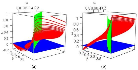
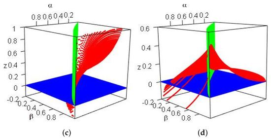Figure 1. Difference surfaces (red), $z=0$ (blue) and $\beta =1-\frac{\overline{C}(\alpha ,\alpha ,\gamma )}{\overline{C}(0,\alpha ,\gamma )}$ (green). (a) ${\widehat{\mathrm{CoVaR}}}_{(\alpha ,\beta ,\gamma )}$$\left(X_2\right|X_1,X_3)-{\widehat{\mathrm{CoVaR}}}_{(\beta ,\alpha ,\gamma )}\left(X_1\right|X_2,X_3$); (b) ${\widehat{\mathrm{CoES}}}_{(\alpha ,\beta ,\gamma )}\left(X_2\right|X_1,X_3)-{\widehat{\mathrm{CoES}}}_{(\beta ,\alpha ,\gamma )}\left(X_1\right|X_2,X_3)$; (c) ${\widehat{\mathsf{\Delta }\mathrm{CoVaR}}}_{(\alpha ,\beta ,\gamma )}\left(X_2\right|X_1,X_3)-{\widehat{\mathsf{\Delta }\mathrm{CoVaR}}}_{(\beta ,\alpha ,\gamma )}\left(X_1\right|X_2,X_3)$; (d) ${\widehat{\mathsf{\Delta }\mathrm{CoES}}}_{(\alpha ,\beta ,\gamma )}\left(X_2\right|X_1,X_3)-{\widehat{\mathsf{\Delta }\mathrm{CoES}}}_{(\beta ,\alpha ,\gamma )}\left(X_1\right|X_2,X_3)$.

As can be seen, the difference is positive for all ${\displaystyle \beta \ge {\beta }_{\alpha }}$, confirming the theoretical finding. Moreover, for some ${\displaystyle \beta <{\beta }_{\alpha }}$, the difference may still be positive.

2.

For $X_1\sim \mathcal{N}(0,1)$, $X_2\sim \mathcal{N}(0,2)$, $X_3\sim \mathcal{N}(0,3)$, there are three normal distributed random risks, according to Table 1.1 of [38], one has $X_1{\le }_{icx}{X}_2$. By the second assertion of Theorem 3, for $\beta \ge {\beta }_{\alpha }$,

$${\mathrm{CoES}}_{(\alpha ,\beta ,\gamma )}\left(X_2\right|X_1,X_3)\ge {\mathrm{CoES}}_{(\beta ,\alpha ,\gamma )}\left(X_1\right|X_2,X_3).$$

Figure 1b shows the difference ${\widehat{\mathrm{CoES}}}_{(\alpha ,\beta ,\gamma )}\left(X_2\right|X_1,X_3)\ge {\widehat{\mathrm{CoES}}}_{(\beta ,\alpha ,\gamma )}\left(X_1\right|X_2,X_3)$, which is positive for $\beta \ge {\beta }_{\alpha }$ and for some $\beta <{\beta }_{\alpha }$.

3.

For $X_1\sim \mathcal{W}(1,1)$, $X_2\sim \mathcal{W}(1.5,1)$, $X_3\sim \mathcal{W}(2,1)$, three Weibull-distributed random risks (The density function of a Weibull-distributed random variable $\mathcal{W}(a,b)$ is given by $(b/a){(x/a)}^{b-1}exp(-{(x/a)}^b)$, where a is the scale parameter, and b is the shape parameter.), as shown in Example 16 of [21], $X_1{\le }_{\mathrm{disp}}{X}_2$. Figure 1c plots the difference ${\widehat{\mathsf{\Delta }\mathrm{CoVaR}}}_{(\alpha ,\beta ,\gamma )}\left(X_2\right|X_1,X_3)-{\widehat{\mathsf{\Delta }\mathrm{CoVaR}}}_{(\beta ,\alpha ,\gamma )}\left(X_1\right|X_2,X_3)$, and the graph also confirms our findings.

4.

For $X_1\sim \mathcal{W}(1,2)$, $X_2\sim \mathcal{W}(1,1)$, $X_3\sim \mathcal{W}(1,3)$, three Weibull-distributed random risks, we have $X_1{\le }_{\mathrm{ew}}{X}_2$ by Example 24 of [21]. Figure 1d plots the difference ${\widehat{\mathsf{\Delta }\mathrm{CoES}}}_{(\alpha ,\beta ,\gamma )}\left(X_2\right|X_1,X_3)-{\widehat{\mathsf{\Delta }\mathrm{CoES}}}_{(\beta ,\alpha ,\gamma )}\left(X_1\right|X_2,X_3)$ and illustrates Theorem 5.

The theoretical findings show that when the underlined dependence structure of the risk portfolio possesses arrangement monotonicity with respect to two random risks, the impact of the stress scenario with the larger marginal risk on the smaller risk is more significant than that of the latter on the former. However, the magnitude of the difference seems to vary significantly, depending on the marginal distributions. In some extreme cases, for example, when the stress levels are both close to 1, the difference may be relatively large. Therefore, in the practice of risk management, simply focusing on the marginal risks and ignoring their dependence structure may lead to an underestimation of the systemic risk level.

6. Concluding Remarks

By capturing the dependence, the co-risk measures and risk contribution measures intuitively reflect the interaction among grouped risks. By extending the comparing results of paired risks [22], this study showed that the potential dependency structure plays a crucial role in determining the risk interaction level of marginal risk between any two risks when there is an arbitrary number of risks. Specifically, when the stress level is high enough, regardless of if the dependence structure is symmetric or arrangement monotonic, a stochastically larger marginal risk will lead to larger $\mathrm{CoVaR}$, $\mathrm{CoES}$, $\mathsf{\Delta }\mathrm{CoVaR}$ and $\mathsf{\Delta }\mathrm{CoES}$, respectively. Moreover, the interaction between two random risks in the case with multiple risks is somewhat surprisingly similar to that obtained in the case with only two random risks.

In their study [39] on measures of risk contagion, Ortega-Jiménez et al. provided a real data example of risk contagion in the Spanish banking sector. It was shown that the asset log returns of Santander bank, the BBVA and Bankinter from June 2015 until June 2019 possess some symmetry dependence structure. Moreover, the asset log returns of BBVA is larger than that of Bankinter in the sense of increasing convex order. Stemming from their example, according to Theorem 3, by using the $\mathrm{CoES}$, we can conclude that more risk stress spread to Bankinter from BBVA than that spread to BBVA from Bankinter. In [16], Tobias and Brunnermeier pointed out that $\mathsf{\Delta }\mathrm{CoVaR}$ can be applied to detect which institution is the most at risk should a financial crisis occur. Along with this finding, Theorem 4 further provides some situations where $\mathsf{\Delta }\mathrm{CoVaR}$ of two specific institutions is comparable when the whole market has more than two.

Our results show that there are potential differences between the interaction levels of marginal risk in multiple risk portfolios. However, there are a few things to be explored: how to calculate the concrete difference between two systemic risks, at least for some specific dependence structure and marginal distribution? Whether there exist cases when a larger random risk results in a smaller systemic risk (As discussed in [40], a bank may not be too big to bankrupt)? What if the underlining dependence structure is neither symmetric nor arrangement monotonic, maybe some asymmetric concepts defined in [41]? The answers to these questions can provide more guidance for the application of common risk measurement and risk contribution measurement in risk management practice and they definitely deserve future study. As pointed out by one reviewer, most of the time, risk comes along with return. It is also interesting to take into consideration financial risk and return simultaneously when studying systemic risk.

References

- Ghosh, B.; Papathanasiou, S.; Ramchandani, N.; Kenourgios, D. Diagnosis and prediction of IIGPS’ countries bubble crashes during BREXIT. Mathematics 2021, 9, 1003. [Google Scholar] [CrossRef]
- Yang, K.; Wei, Y.; He, J.; Li, S. Dependence and risk spillovers between mainland China and London stock markets before and after the Stock Connect programs. Phys. A Stat. Mech. Its Appl. 2019, 526, 120883. [Google Scholar] [CrossRef]
- Zhu, B.; Zhou, X.; Liu, X.; Wang, H.; He, K.; Wang, P. Exploring the risk spillover effects among China’s pilot carbon markets: A regular vine copula-CoES approach. J. Clean. Prod. 2020, 242, 118455. [Google Scholar] [CrossRef]
- Acerbi, C.; Nordio, C.; Sirtori, C. Expected shortfall as a tool for financial risk management. arXiv 2001, arXiv:0102304. [Google Scholar]
- Acerbi, C.; Tasche, D. On the coherence of expected shortfall. J. Bank. Financ. 2002, 26, 1487–1503. [Google Scholar] [CrossRef]
- Artzner, P.; Delbaen, F.; Eber, J.M.; Heath, D. Coherent measures of risk. Math. Financ. 1999, 9, 203–228. [Google Scholar] [CrossRef]
- Yamai, Y.; Yoshiba, T. Value-at-risk versus expected shortfall: A practical perspective. J. Bank. Financ. 2005, 29, 997–1015. [Google Scholar] [CrossRef]
- Chen, S.X. Nonparametric estimation of expected shortfall. J. Financ. Econom. 2008, 6, 87–107. [Google Scholar] [CrossRef]
- Righi, M.B.; Ceretta, P.S. A comparison of Expected Shortfall estimation models. J. Econ. Bus. 2015, 78, 14–47. [Google Scholar] [CrossRef]
- Denuit, M.; Dhaene, J.; Goovaerts, M.; Kaas, R. Actuarial Theory for Dependent Risks: Measures, Orders and Models; John Wiley & Sons: Hoboken, NJ, USA, 2006. [Google Scholar]
- Jorion, P. Value at Risk: The New Benchmark for Managing Financial Risk; McGraw-Hill: New York, NY, USA, 2000. [Google Scholar]
- Embrechts, P.; Höing, A.; Puccetti, G. Worst var scenarios. Insur. Math. Econ. 2005, 37, 115–134. [Google Scholar] [CrossRef]
- Kaas, R.; Laeven, R.J.; Nelsen, R.B. Worst VaR scenarios with given marginals and measures of association. Insur. Math. Econ. 2009, 44, 146–158. [Google Scholar] [CrossRef]
- Laeven, R.J. Worst VaR scenarios: A remark. Insur. Math. Econ. 2009, 44, 159–163. [Google Scholar] [CrossRef][Green Version]
- Girardi, G.; Ergün, A.T. Systemic risk measurement: Multivariate GARCH estimation of CoVaR. J. Bank. Financ. 2013, 37, 3169–3180. [Google Scholar] [CrossRef]
- Adrian, T.; Brunnermeier, M.K. CoVaR. Am. Econ. Rev. 2016, 106, 1705–1741. [Google Scholar] [CrossRef]
- Mainik, G.; Schaanning, E. On dependence consistency of CoVaRand some other systemic risk measures. Stat. Risk Model. 2014, 31, 49–77. [Google Scholar] [CrossRef]
- Caporin, M.; Costola, M.; Garibal, J.C.; Maillet, B. Systemic risk and severe economic downturns: A targeted and sparse analysis. J. Bank. Financ. 2022, 134, 106339. [Google Scholar] [CrossRef]
- Jiang, Y.; Mu, J.; Nie, H.; Wu, L. Time-frequency analysis of risk spillovers from oil to BRICS stock markets: A long-memory Copula-CoVaR-MODWT method. Int. J. Financ. Econ. 2022, 27, 3386–3404. [Google Scholar] [CrossRef]
- Mao, T.; Zhao, Q.; Wu, Q. Worst-case conditional value-at-risk and conditional expected shortfall based on covariance information. JUSTC 2022, 52, 4. [Google Scholar] [CrossRef]
- Sordo, M.A.; Bello, A.J.; Suárez-Llorens, A. Stochastic orders and co-risk measures under positive dependence. Insur. Math. Econ. 2018, 78, 105–113. [Google Scholar] [CrossRef]
- Fang, R.; Li, X. Some results on measures of interaction between paired risks. Risks 2018, 6, 88. [Google Scholar] [CrossRef]
- Shaked, M.; Shanthikumar, J.G. Stochastic Orders; Springer: Berlin/Heidelberg, Germany, 2007. [Google Scholar]
- Belzunce, F.; Riquelme, C.M.; Mulero, J. An Introduction to Stochastic Orders; Academic Press: New York, NY, USA, 2015. [Google Scholar]
- Li, H.; Li, X. Stochastic orders in reliability and risk. In Honor of Professor Moshe Shaked; Springer: New York, NY, USA, 2013. [Google Scholar]
- Shaked, M.; Shanthikumar, J.G. (Eds.) Univariate Stochastic Orders. In Stochastic Orders; Springer New York: New York, NY, USA, 2007; pp. 3–79. [Google Scholar] [CrossRef]
- Sordo, M.A.; Ramos, H.M. Characterization of stochastic orders by L-functionals. Stat. Pap. 2007, 48, 249–263. [Google Scholar] [CrossRef]
- Balbás, A.; Garrido, J.; Mayoral, S. Properties of distortion risk measures. Methodol. Comput. Appl. Probab. 2009, 11, 385–399. [Google Scholar] [CrossRef]
- Glynn, P.W.; Peng, Y.; Fu, M.C.; Hu, J.Q. Computing sensitivities for distortion risk measures. INFORMS J. Comput. 2021, 33, 1520–1532. [Google Scholar] [CrossRef]
- Nelsen, R.B. An Introduction to Copulas; Springer Science & Business Media: Berlin/Heidelberg, Germany, 2007. [Google Scholar]
- Cai, J.; Wei, W. On the invariant properties of notions of positive dependence and copulas under increasing transformations. Insur. Math. Econ. 2012, 50, 43–49. [Google Scholar] [CrossRef]
- Karimalis, E.N.; Nomikos, N.K. Measuring systemic risk in the European banking sector: A copula CoVaR approach. Eur. J. Financ. 2018, 24, 944–975. [Google Scholar] [CrossRef]
- Kim, J.S.; Proschan, F. A review: The arrangement increasing partial ordering. Comput. Oper. Res. 1995, 22, 357–371. [Google Scholar] [CrossRef]
- Barlow, R.E.; Proschan, F. Statistical Theory of Reliability and Life Testing: Probability Models; Holt, Rinehart & Winston: New York, NY, USA, 1975. [Google Scholar]
- Metropolis, N.; Ulam, S. The monte carlo method. J. Am. Stat. Assoc. 1949, 44, 335–341. [Google Scholar] [CrossRef]
- Rubinstein, R.Y.; Kroese, D.P. Simulation and the Monte Carlo Method; John Wiley & Sons: Hoboken, NJ, USA, 2016. [Google Scholar]
- McNeil, A.J.; Frey, R.; Embrechts, P. Quantitative Risk Management: Concepts, Techniques and Tools-Revised Edition; Princeton University Press: Princeton, NJ, USA, 2015. [Google Scholar]
- Mccomb, M.A. Comparison Methods for Stochastic Models and Risks. Techometrics 2003, 45, 370–371. [Google Scholar] [CrossRef]
- Ortega-Jiménez, P.; Sordo, M.; Suárez-Llorens, A. Stochastic orders and multivariate measures of risk contagion. Insur. Math. Econ. 2021, 96, 199–207. [Google Scholar] [CrossRef]
- Zhou, C. Are Banks Too Big to Fail? Measuring Systemic Importance of Financial Institutions. Int. J. Cent. Bank. 2010, 6, 46. [Google Scholar] [CrossRef]
- Raineri, L.; Shanske, D. Municipal Finance and Asymmetric Risk. Belmont Law Rev. 2017, 4, 65. [Google Scholar]
Publisher’s Note: MDPI stays neutral with regard to jurisdictional claims in published maps and institutional affiliations. |
© 2022 by the authors. Licensee MDPI, Basel, Switzerland. This article is an open access article distributed under the terms and conditions of the Creative Commons Attribution (CC BY) license (https://creativecommons.org/licenses/by/4.0/).