A Matrix Approach to the Modeling and Analysis of Network Evolutionary Games with Mixed Strategy Updating Rules

Abstract

So far, most studies on networked evolutionary game have focused on a single update rule. This paper investigated the seeking of the Nash Equilibrium and strategy consensus of the evolutionary networked game with mixed updating rules. First, we construct the algebraic formulation for the dynamics of the evolutionary networked game by using the semi-tensor product method. Second, based on the algebraic form, the dynamic behavior of networked evolutionary games is discussed, and an algorithm to seek the Nash equilibrium is proposed. Third, we investigate the strategy consensus problem for a special networked evolutionary game. Finally, some illustrative examples are given to verify our conclusions.

1. Introduction

Game theory, introduced by Von et al. [1], is the study of disciplines that deal with the decision-making problems. Considering the update of strategy profiles with respect to time, biologists Smith and Price proposed the evolutionary game theory in [2]. Later, paper [2,3,4] demonstrated that players naturally evolved towards a higher-return goal or higher fitness following a series of adaptive learning processes based on specific rules, eventually reaching a steady state, which was called the Evolutionary Stable Strategy (ESS) [2]. The fundamental principle in the majority of early literature in evolutionary games was that individuals interact with all the other players. Arefin et al. [5] investigated the social dilemmas by the social efficiency deficit without the spatial structure. In the literature [6,7], the authors investigated the network adaptation dynamics of the Prisoner’s Dilemma game and the Public Goods game, respectively. Both papers demonstrated that the cooperation was actually enhanced when the network structure was taken into account. Moreover, in many practical situations, an individual only just interacts with its neighbors, such as its friends, relatives, colleagues. Due to this, Nowak and May proposed the concept of the networked evolutionary game (NEG) [8] by adding a network into the classical framework of games. In the network, nodes represent players and edges denote the relationship among players.

Recently, networked evolutionary games have been applied to many real-life decision-making problems such as the plastic ban problem in [9] and the epidemiological problems in [10]. Among the study of NEGs, a very interesting and fundamental issue is the analysis of the evolutionary trends for all players’ behaviors and the problem of the seeking strategy Nash Equilibrium. It is noted that the current works on networked evolutionary games are mainly based on mean-field techniques [11] and computer simulations [12]. However, using these methods to investigate the evolution of game dynamics from a strictly theoretical point of view is quite challenging.

Professor Cheng recently introduced a new matrix product, that is the semi-tensor product (STP) of matrices to relax the general matrix product restriction on dimensionality and could effectively handle the logic network problems. Many papers [13,14,15] applied this method to NEGs by converting logical functions into algebraic forms, which makes the problem identical to that in the control. Cheng et al. [16,17] investigated the fundamental theoretical framework for analyzing and controlling NEGs and they demonstrated that if the strategy update rule (SUR), where each player decides his action in the following step based on the knowledge about its neighbors, is one of the most critical factors of network evolutionary games. Once the SUR is determined, the evolution progress will be determined accordingly. The most popular SURs currently are the Myopic best response adjustment rule (MBRA) [18], Unconditional Imitation [8], Fermi Rule [19]. For example, some authors [20,21,22] have discussed a class of NEGs under the MBRA rule and established the corresponding algebraic formulation of the game.

It is worth noting that players may update their choices according to more than one rule. For instance, when customers purchase a product in the market, they may not be familiar with the market or may not be aware of whether the merchant’s pricing is high or typical, so they will rely on their own experiences or the recommendations of their friends. The merchant in this game may use several sales strategies to obtain a high revenue. The papers [23,24] investigated the dynamics based on a well-mixed population under mixed rules.

Based on the above-mentioned discussions, we present the model of networked evolutionary with mixed updating rules. The following list summarizes the main contributions of this study.

• This paper puts forward a new evolutionary networked game model called the Mixed Rules NEG. This model can well describe the real situation in which players adopt mixed rules to play with its neighbors in reality.
• We give two strategy updating rules and establish their strict algebraic forms by the method STP. Then, we construct the algebraic expression of the evolutionary process under mixed rules.
• We discuss the Nash Equilibrium under the game.
• A class of networked game’s strategy optimization is discussed. We obtain two results on whether and when the game will achieve an optimal strategy.

The remainder the paper is organized as follows. Section 2 contains some necessary preliminaries on the NEG and semi-tensor product. In Section 3, we present the main results of this paper. Then, we provide two illustrative examples in Section 4, which is followed by the conclusion in Section 5.

2. Preliminaries

In this section, we give some necessary preliminaries, which will be used in the sequel.

2.1. Semi-Tensor Product

Before recalling the STP of matrices, some concepts are listed as follows.

(1)

$\mathbb{R}$ is the field of real numbers;

(2)

${\mathbb{R}}^n$ is the n dimensional Euclidean space;

(3)

${\mathbb{M}}_{m\times n}$ is the set of $m\times n$ real matrices;

(4)

$Co{l}_i\left(M\right)$ is the i-th column of matrix M; $Col\left(M\right)$ is the set of columns of M;

(5)

$Ro{w}_i\left(M\right)$ is the i-th column of matrix M; $Row\left(M\right)$ is the set of columns of M;

(6)

$V_r\left(A\right)={(a_{11},\dots ,a_{1n},\dots ,a_{m1},\dots ,a_{mn})}^T$ denotes the row stacking form of A;

(7)

${\mathrm{\Delta }}_n:=Col\left(I_n\right);{\delta }_n^i:=Co{l}_i\left(I_n\right)\in {\mathrm{\Delta }}_n$;

(8)

$M\in {\mathcal{M}}_{m\times n}$ is called a logical matrix if the columns of L are the form of ${\delta }_n^k$. That is, Col (L)$\subset {\mathrm{\Delta }}_m$. Denote by ${\mathcal{L}}_{m\times n}$ the set of $m\times n$ logical matrices;

(9)

Assume $L\in {\mathcal{L}}_{m\times n}$, then $L=[{\delta }_m^{i_1},{\delta }_m^{i_2},\dots ,{\delta }_m^{i_m}]$, and its shorthand form is $L={\delta }_m[i_1{i}_2\dots i_n]$;

(10)

$r=[r_1,\dots ,r_k]\in {\mathbb{R}}^k$ is a probabilistic vector, if $r_i\ge 0,i=1,\dots ,k$, and ${\displaystyle \sum _{i=1}^k}{r}_i=1$. The set of k dimensional probabilistic vectors is denoted by ${\gamma }_k$. The set of $m\times n$ probabilistic matrices is denoted by ${\gamma }_{m\times n}$.

(11)

$1_k:={\underset{k}{\underbrace{[11\cdots 1]}}}^T$.

The STP of matrices is the fundamental tool in our approach. We provide a brief review here and refer to [15] for details.

Definition 1.

Let $A\in {\mathbb{R}}^{m\times n}$ and $B\in {\mathbb{R}}^{p\times q}$. Then, we define the STP of A and B as [15]

$$A⋉B:=(A\otimes I_{\frac{t}{n}})(B\otimes I_{\frac{t}{p}})\in {\mathcal{R}}_{\frac{mt}{n}\times \frac{qt}{p}}.$$

(1)

where $t=lcm(n,p)$ is the least common multiple of n and p.

Lemma 1.

Assume $X\in {\mathbb{R}}^m$ and $Y\in {\mathbb{R}}^n$. Define two matrices, named by ‘delete rear operator’ and ‘delete front operator’ respectively, as $D_r^{m,n}=I_m\otimes 1_n^T$, $D_f^{m,n}=1_n^T\otimes I_m$. Then, we have [15]

$$D_r^{m,n}⋉X⋉Y=X$$

(2)

$$D_f^{m,n}⋉X⋉Y=Y.$$

(3)

The following are some special properties of STP, which will be used in the sequel.

Definition 2.

A swap matrix $W_{[m,n]}\in {\mathbb{R}}_{mn\times mn}$ is defined as follows:

$$\begin{array}{cc}\hfill W_{[m,n]}:={\delta }_{mn}& [1m+1\dots (n-1)m+1\hfill \\ \hfill & 2m+2\dots (n-1)m+2\hfill \\ \hfill & \cdots \hfill \\ \hfill & mm+m\dots (n-1)m+m].\hfill \end{array}$$

If m = n, it can be expressed briefly as $W_{\left[n\right]}$.

Proposition 1.

Let A be a matrix, $X\in {\mathbb{R}}^{m\times 1}$ and $Y\in {\mathbb{R}}^{n\times 1}$ be two column vectors, $x\in {\mathrm{\Delta }}_p$ and $x_i\in {\mathrm{\Delta }}_k$, $i=1,2,\dots ,n$. Then

$$X⋉A=(I_m\otimes A)⋉X;$$

(4)

$$Y⋉X=W_{[m,n]}⋉X⋉Y;$$

(5)

Proposition 2.

Let $f(x_1,\dots ,x_n):{\mathrm{\Delta }}_k^n\left({\gamma }_k^n\right)\to {\mathrm{\Delta }}_k\left({\gamma }_k\right)$ be a finite-valued mapping. Then, there exists a unique matrix $M_f\in {\mathcal{L}}_{k\times k^n}\left({\gamma }_{k\times k^n}\right)$, such that

$$f(x_1,\dots ,x_n)=M_{f}x,$$

(6)

where $x={⋉}_{j=1}^n{x}_j$.

Remark 1.

The STP is the ordinary matrix product when q=m, which keeps all original properties of ordinary matrix product. In this paper, the matrix product is assumed to be STP, and without confusion, one can omit the symbol ‘⋉’ and simply call it `product’.

2.2. Networked Evolutionary Game

We briefly recall the basic concepts of NEGs, proposed in [17].

Definition 3.

A fundamental network game (FNG) is consisted of three factors (N, S, C).

1.

$N:=\{1,2\}$ denotes the players’ set;

2.

$S:=\{s_1,s_2,\dots ,s_k\}$ denotes the strategy set;

3.

$C:={\left(c_{ij}\right)}_{k\times k}$ denotes the payoff matrix, element $c_{ij}$ denotes the payoff of when player 1 takes strategy $s_i$ and player 2 takes strategy $s_j$.

If A satisfy $c_{ij}=c_{ji}$, then we say this is a symmetric game.

Definition 4.

A networked evolutionary game (NEG) consists of the following factors.

• A topology about the network, denoted by a undirected graph $(\mathcal{V},\mathcal{E})$, where $\mathcal{V}=\{1,\dots ,n\}$ denotes the nodes, $\mathcal{E}\in \mathcal{V}\times \mathcal{V}$ denotes the vertex. There is a adjacent matrix $A={\left(a_{ij}\right)}_{n\times n}$ corresponding to the graph, if there is a edge between i and j, then $a_{ij}=1$, otherwise, $a_{ij}=0$. Denote by $N_i$ the neighborhood of player i where $j\in N_i$ if and only if $(i,j)\in \mathcal{E}$;
• A fundamental network game G, such that if $(i,j)\in \mathcal{E}$, then player i and j play FNG with strategies $x_i\left(t\right)\in S$ and $x_j\left(t\right)\in S$, respectively;
• A strategy updating rule (SUR) $F=\{f_1,f_2,\dots ,f_n\}$, that is, player i takes the rule $f_i$ to determine the next step’s strategy, i.e.,

$$x_i(t+1)=f_i(x_0\left(t\right),x_1\left(t\right),\dots ,x_n\left(t\right)),x_i\left(t\right)\in S$$

Remark 2.

We can observe from Lemma 2 that for every update rule, the existence and uniqueness of the strategy updating matrix can be guaranteed.

In addition, there are some SURs we will use in the sequel.

(I)

(Myopic best response adjustment rule) Each player holds the opinion that its neighbors will make the same decisions as in their last step, and the strategy choice at the present time is the best response against its neighbors’ strategies in the last step. It can be expressed as

$$x_i(t+1)=x_{j_i}\left(t\right),$$

(7)

$$j_i\in \underset{j\in N_i\cup \left\{i\right\}}{argmax}\left\{p_j\left(t\right)\right\}:=Q_i.$$

(8)

If the $argmax$ set is not a singleton, then we choose the minimum, i.e., $x_i(t+1)=x_{min{Q}_i}\left(t\right)$.

(II)

(Unconditional Imitation Rule) Each player adopts the strategy of the player with the largest gain in the neighborhood at the initial moment, i.e.,

$$x_i(t+1)=x_{j_i}\left(t\right),$$

(9)

$$j_i\in \underset{j\in N_i\cup \left\{i\right\}}{argmax}\left\{p_j(x_j\left(0\right),x_k\left(0\right)|k\in N_k)\right\},$$

(10)

In addition, we adopt the same priority as rule (I).

(III)

(Repeating Rule) Each player will choose the same strategy as the last step, i.e.,

$$x_i(t+1)=x_i\left(t\right),\forall t>0,i\in N.$$

(11)

3. Main Result

3.1. Problem Formulation

In this paper, we consider a network game, and assume that it can repeat infinitely. At each time, player i only competes with its neighbors. We use $p_i(x_i\left(t\right),x_j\left(t\right)|j\in N_i)$ to denote its aggregate payoff. Then, it can be expressed as

$$p_i(x_i\left(t\right),x_j\left(t\right)|j\in N_i)=\sum _{j\in N_i}{p}_{ij}(x_i\left(t\right),x_j\left(t\right)),$$

(12)

where $p_{ij}(x_i\left(t\right),x_j\left(t\right))$ denotes the payoff in the game of player i with its neighbor j when i takes strategy $x_i\left(t\right)$ and j takes strategy $x_j\left(t\right)$. The NEG is evolved with the above three different SURs simultaneously, which makes the evolutionary dynamics more complicated and more consistent with the actual situation.

3.2. Mixed Rules NEG Dynamics

We assume that each player considers that its neighbors will adopt rules (I)–(III) with the probability $\alpha ,\beta ,\gamma$, respectively, and these three parameters satisfy $\alpha +\beta +\gamma =1$. All the players are eager to gain the maximum payoff. Then, we will establish the algebraic forms of the NEG dynamics in the following.

Using semi-tensor product method, for any $i\in \mathcal{V}$, we identify $i\sim {\delta }_n^i,i=1,2,\dots ,n.$ Then, $\mathcal{V}\sim {\mathrm{\Delta }}_n,x_i\left(t\right)\sim {\mathrm{\Delta }}_k$ and $x\left(t\right)={⋉}_{i=1}^n{x}_i\left(t\right)\sim {\mathrm{\Delta }}_{k^n}$.

Lemma 2.

Define a matrix $\mathrm{\Pi }={[{\left({\pi }_n^1\right)}^T,{\left({\pi }_n^2\right)}^T,\dots ,{\left({\pi }_n^{n-1}\right)}^T]}^T$, where ${\pi }_n^j=D_r^{k,k^{n-j-1}}{D}_f^{k^{j-1},k},j=1,2,\dots ,n-1.$ We have $\mathrm{\Pi }{x}_{-i}\left(t\right)={[{\left(x_1\left(t\right)\right)}^T,\dots ,{\left(x_{i-1}\left(t\right)\right)}^T,{\left(x_{i+1}\left(t\right)\right)}^T,\dots ,{\left(x_n\left(t\right)\right)}^T]}^T.$

Then, let us discuss the evolutionary dynamics under three rules, respectively.

(A)

If player i chooses rule (I), we can transform the payoff function into algebraic form by the first rule as follows

$$\begin{array}{cc}\hfill p_i\left(t\right)& =\sum _{j\in N_i}{p}_{ij}(x_i\left(t\right),x_j\left(t\right))\hfill \\ \hfill & =V_r^T\left(C\right)x_i\left(t\right)\sum _{j\in N_i}{x}_j\left(t\right)\hfill \\ \hfill & =V_r^T\left(C\right)x_i\left(t\right)Ro{w}_i\left(A_i\right)\mathrm{\Pi }{x}_{-i}\left(t\right)\hfill \\ \hfill & =V_r^T\left(C\right)\left[I_k\otimes Ro{w}_i\left(A_i\right)\mathrm{\Pi }\right]x_i\left(t\right)x_{-i}\left(t\right)\hfill \\ \hfill & =V_r^T\left(C\right)\left[I_k\otimes Ro{w}_i\left(A_i\right)\mathrm{\Pi }\right]W_{[k^{n-1},k]}{x}_{-i}\left(t\right)x_i\left(t\right)\hfill \\ \hfill & :=R_i{x}_{-i}\left(t\right)x_i\left(t\right),\hfill \end{array}$$

(13)

where $A_i$ is the matrix A excepted the i-th column and $x_{-i}=x_1⋉\dots ⋉x_{i-1}⋉x_{i+1}⋉\dots ⋉x_n$. We can divide $R_i$ into $k^{n-1}$ blocks as

$$R_i=[Bl{k}_1\left(R_i\right),Bl{k}_2\left(R_i\right),\dots ,Bl{k}_{k^{n-1}}\left(R_i\right)],$$

(14)

The r-th block means player i’s payoff when others’ strategy profile is $x_{-i}\left(t\right)={\delta }_{k^{n-1}}^j$ at time t. We deduce the best response strategies of all the other players by letting

$$s_{i,j}=min\underset{q=1,\dots ,k}{argmax}Co{l}_q\left(Bl{k}_j\left(R_i\right)\right),j=1,\dots ,k^{n-1}.$$

(15)

$s_{i,j}$ means the player i’s best response strategy when others strategy profile $x_{-i}={\delta }_{k^{n-1}}^j$. Let $L_i={\delta }_k[s_{i,1},s_{i,2},\dots ,s_{i,k^{n-1}}]$, the algebraic forms of strategy dynamics of player i can be expressed as:

$$\begin{array}{cc}\hfill x_i(t+1)& =L_i{x}_{-i}\left(t\right)\hfill \\ \hfill & =L_i{D}_f^{k,k}{W}_{[k^{i-1},k]}x\left(t\right)\hfill \\ \hfill & :=L_i^{\left(1\right)}x\left(t\right).\hfill \end{array}$$

(16)

(B)

If player i chooses rule (II), we need an initial strategy profile, and we assume that player i’s neighbor $j_i$ has the maximum payoff at the initial time, then we can imply the dynamics of player i as:

$$\begin{array}{cc}\hfill x_i(t+1)& =x_{j_i}\left(t\right)\hfill \\ \hfill & =D_r^{k,k^{n-j_i}}{D}_f^{k^{j_i-1},k^{n-j_i}}x\left(t\right)\hfill \\ \hfill & :=L_i^{\left(2\right)}x\left(t\right).\hfill \end{array}$$

(17)

We can find that the dynamics of rule (II) needs the initial strategy profile.

(C)

If player i chooses rule (III), its strategy dynamics can be expressed as

$$\begin{array}{cc}\hfill x_i(t+1)& =x_i\left(t\right)\hfill \\ \hfill & =D_r^{k,k^{n-i}}{D}_f^{k^{i-1},k^{n-i+1}}x\left(t\right)\hfill \\ \hfill & :=L_i^{\left(3\right)}x\left(t\right).\hfill \end{array}$$

(18)

Let us establish the algebraic forms of the payoff function of player i as:

$$\begin{array}{cc}\hfill p_i\left(t\right)& =\sum _{j\in N_i}{p}_{ij}(x_i\left(t\right),x_j\left(t\right))\hfill \\ \hfill & =V_r^T\left(C\right)x_i\left(t\right)\sum _{j\in N_i}\alpha x_j^{\left(1\right)}\left(t\right)+\beta x_j^{\left(2\right)}\left(t\right)+\gamma x_j^{\left(3\right)}\left(t\right)\hfill \\ \hfill & =V_r^T\left(C\right)W_{[k,k]}\left(\sum _{j\in N_i}\alpha x_j^{\left(1\right)}\left(t\right)+\beta x_j^{\left(2\right)}\left(t\right)+\gamma x_j^{\left(3\right)}\left(t\right)\right)x_i\left(t\right)\hfill \\ \hfill & =V_r^T\left(C\right)W_{[k,k]}\left(\sum _{j\in N_i}\alpha L_j^{\left(1\right)}+\beta L_j^{\left(2\right)}+\gamma L_j^{\left(3\right)}\right)x(t-1)x_i\left(t\right)\hfill \\ \hfill & =V_r^T\left(C\right)W_{[k,k]}Ro{w}_i\left(A\right)L\left[\begin{array}{c}\alpha \\ \beta \\ \gamma \end{array}\right]x(t-1)x_i\left(t\right)\hfill \\ \hfill & :=R_i^{\prime }x(t-1)x_i\left(t\right)\hfill \end{array}$$

(19)

where

$$\begin{array}{c}\hfill L=\left[\begin{array}{ccc}{L}_1^{\left(1\right)}& L_1^{\left(2\right)}& L_1^{\left(3\right)}\\ L_2^{\left(1\right)}& L_2^{\left(2\right)}& L_2^{\left(3\right)}\\ ⋮& ⋮& ⋮\\ L_n^{\left(1\right)}& L_n^{\left(2\right)}& L_n^{\left(3\right)}\end{array}\right],\end{array}$$

(20)

Then we divide $R_i^{\prime }$ into $k^n$ blocks as,

$$R_i^{\prime }=[Bl{k}_1\left(R_i^{\prime }\right),Bl{k}_2\left(R_i^{\prime }\right),\dots ,Bl{k}_{k^n}\left(R_i^{\prime }\right)]$$

(21)

The r-th blocks means player i’s payoff when the strategy profile of the last step $x(t-1)={\delta }_{k^n}^r$. We deduce the best response strategies of all other players by letting

$$s_{i,j}=min\underset{q=1,\dots ,k}{argmax}Co{l}_q\left(Bl{k}_j\left(R_i^{\prime }\right)\right),j=1,\dots ,k^n.$$

(22)

Let $T_i={\delta }_k[s_{i1},s_{i2},\dots ,s_{i{k}^n}]$, the algebraic forms of strategy dynamics of player i can be expressed as:

$$x_i(t+1)=T_{i}x\left(t\right),i=1,2,\dots ,n.$$

(23)

By multiplying all the n equations together, we have the algebraic state space form of the strategy profile dynamics as:

$$x(t+1)=Tx\left(t\right),$$

(24)

where $Co{l}_i\left(T\right)=Co{l}_i\left(T_1\right)Co{l}_i\left(T_2\right)\dots Co{l}_i\left(T_n\right),i=1,\dots ,k^n$.

Remark 3.

There are two payoff Functions (13) and (19), the first one means the actual earning and the second one means the expected earning. As a matter of fact, the second one is more closed to reality.

It is noted that the algebraic Form (24) contains all the characteristics of the game, in other words, we can study the properties of the mixed strategy updating rules through the matrix T. The advantage of using the semi-tensor product is that the dynamical progress can be implied to the algebraic form, which helps us analyze the NEGs mathematically.

3.3. Nash Equilibrium Seeking

In this part, we will discuss the Nash equilibrium of the normal game. At first, we give the definition of the Nash equilibrium.

Definition 5.

The strategy profile $x^{*}\in S_i\times S_2\times \cdots \times S_n$ is called a Nash equilibrium, if

$$p_i(x_i^{*},x_{-i}^{*})\ge p_i(x_i,x_{-i}^{*})$$

(25)

holds for any $x_i\in S_i$ and $i\in N$, where $N=\{1,\dots ,n\}$ is the set of players, $p_i$ and $S_i$ are the payoff function and the set of strategies of the player i, respectively. $x^{*}=(x_1^{*},\dots ,x_n^{*})$ and $x_{-i}^{*}=(x_1^{*},\dots ,x_{i-1}^{*},x_{i+1}^{*},\dots ,x_n^{*})$ [25].

Remark 4.

If (25) holds when $x_i^{*}\in {\mathrm{\Delta }}_k$ for any $i\in N$, then we say $x^{*}$ is a pure Nash equilibrium (PNE), and if $x_i^{*}\in {\gamma }_k$, then it is a mixed Nash equilibrium (MNE). In this paper, we only consider the PNE.

Due to the uncertainty about the SUR used by the other players, each player makes their decision in the next step based on the expected profits of others under the mixed SURs. As a result, the study of the Nash Equilibrium is consistent with the expected profits, as in Equation (19).

Theorem 1.

Consider a given NEG $\left(\right(\mathcal{V},\mathcal{E}),G,F)$. The algebraic forms of payoff functions are shown in Equation (13). There exists a NE in the game if and only if d has a non-negative column, that is, $\exists 1\le j\le k^n$, such that

$$Co{l}_j\left(\mathcal{D}\right)\ge 0,$$

(26)

where

$$\begin{array}{cc}\hfill {\mathcal{D}}_i& ={({\mathcal{D}}_{i,1}^T,\dots ,{\mathcal{D}}_{i,k-1}^T)}^T,\hfill \\ \hfill {\mathcal{D}}_{i,r}& =R_i[I_{k^{n-1}}\otimes (I_k-M^r)]W_{[k^{n-1},k]}{W}_{[k,k^{i-1}]},\hfill \end{array}$$

(27)

for $1\le r\le k-1$, and $M={\delta }_k[23\dots k1]$. Moreover, the set of all NEs is

$$\left\{{\delta }_{k^n}^j\right|Co{l}_j\left(\mathcal{D}\right)\ge 0,1\le j\le k^n\}$$

(28)

Proof. (Necessity). Assume that strategy profile $(x_1,\dots ,x_n)$ is a NE of the game. Then, according to Definition 5, for any $x_i^{\prime }\in S_i$, we have

$$p_i(x_{-i},x_i)-p_i(x_{-i},x_i^{\prime })\ge 0,\forall i=1,2,\dots ,n.$$

(29)

For a given strategy $x_i^{\prime }\in S_i$ of player i and $x_i^{\prime }\ne x_i$, it is easy to see that there must exist a $1\le r\le k-1$, such that $x_i^{\prime }=M^r{x}_i$. When r goes from 1 to $k-1$, one can obtain all possible strategies $x_i^{\prime }\in S_i$ and $x_i^{\prime }\ne x_i$.

Then, for each r, we have

$$\begin{array}{cc}\hfill & p_i(x_{-i},x_i)-p_i(x_{-i},x_i^{\prime })\hfill \\ \hfill & =R_i^{\prime }{x}_{-i}\left(t\right)x_i\left(t\right)-R_i^{\prime }{x}_{-i}\left(t\right)M^r{x}_i\left(t\right)\hfill \\ \hfill & =R_i^{\prime }{x}_{-i}\left(t\right)x_i\left(t\right)-R_i^{\prime }(I_{k^{n-1}}\otimes M^r)x_{-i}\left(t\right)x_i\left(t\right)\hfill \\ \hfill & =R_i^{\prime }(I_{k^n}-I_{k^{n-1}}\otimes M^r)x_{-i}\left(t\right)x_i\left(t\right)\hfill \\ \hfill & =R_i^{\prime }(I_{k^n}-I_{k^{n-1}}\otimes M^r)W_{[k^{n-1},k]}{W}_{[k,k^{i-1}]}x\left(t\right)\hfill \\ \hfill & =R_i^{\prime }[I_{k^{n-1}}\otimes (I_k-M^r)]W_{[k^{n-1},k]}{W}_{[k,k^{i-1}]}x\left(t\right)\hfill \\ \hfill & ={\mathcal{D}}_{i,r}x\left(t\right)\ge 0,\hfill \end{array}$$

(30)

where $x_{-i}\in {\mathrm{\Delta }}_{k^{n-1}},x_i\in {\mathrm{\Delta }}_k,{\mathcal{D}}_{i,r}\in {\mathbb{R}}^{1\times k^n}$.

Construct the matrix ${\mathcal{D}}_i$ for player i as

$${\mathcal{D}}_i={({\mathcal{D}}_{i,1}^T,{\mathcal{D}}_{i,2}^T,\dots ,{\mathcal{D}}_{i,k-1}^T)}^T,$$

(31)

And

$$\mathcal{D}={({\mathcal{D}}_1^T,{\mathcal{D}}_2^T,\dots ,{\mathcal{D}}_n^T)}^T.$$

(32)

We can find that the j-th column of ${\mathcal{D}}_{i,r}$ denotes the difference of player i’s payoff between $(x_1,\dots ,x_n)$ and $(x_1,\dots ,x_{i-1},M^r{x}_i,x_{i+1},\dots ,x_n)$. Thus, if the strategy is ${\delta }_{k^n}^j$, then the j-th column of ${\mathcal{D}}_{i,r}$ is more than zero. Similarly, we can obtain $Co{l}_j\left(\mathcal{D}\right)\ge 0$, and ${\delta }_{k^n}^j$ is a NE.

(Sufficiency). Assume that (30) holds. By the proof of the necessity, it implies that strategy profile x satisfy (25). Thus x is a NE of game.    □

Remark 5.

According to the above theorem, if the structure matrix $R_i$ of the game reward is known, the aforementioned theorem can solve all pure Nash equilibrium of the game directly.

Remark 6.

The aforementioned computation shows that the network between the players as well as the players’ payoff are both relevant to the Nash Equilibrium (Algorithm 1).

Algorithm 1: Seeking of Nash Equilibrium.

Step 1: Calculate the payoff matrices $R_i^{\prime }=V_r^T\left(C\right)W_{\left[k\right]}Ro{w}_i\left(A\right)L\left[\begin{array}{c}\alpha \\ \beta \\ \gamma \end{array}\right],i=1,\dots ,n.$ Step 2: Calculate the difference matrices ${\mathcal{D}}_{i,r}=R_i^{\prime }[I_{k^{n-1}}\otimes (I_k-M^r)]W_{[k^{n-1},k]}{W}_{[k,k^{i-1}]},r=1,\dots ,k-1,i=1,\dots ,n.$ Step 3: Establish the judging matrix $\mathcal{D}={[{\mathcal{D}}_{1,1}^T,{\mathcal{D}}_{1,2}^T,\dots ,{\mathcal{D}}_{1,k-1}^T,\dots ,{\mathcal{D}}_{n,1}^T,\dots ,{\mathcal{D}}_{n,k-1}^T]}^T.$ Step 4: Find all the non-negative columns of matrix $\mathcal{D}$.

3.4. Strategy Consensus Analysis

In this part, we consider a special situation as [20], where the cost matrix $C\in {\mathcal{R}}^{n\times n}$ satisfies $c_{jj}=\underset{1\le i\le k}{max}{c}_{ij},\forall 1\le j\le k$, and $a_{kk}=\underset{1\le i\le k}{max}{c}_{ii}$. Then, we will provide two results whether and when the above game will achieve the optimal strategy profile. Moreover, one can use Theorem 1 to verify whether it is a NE.

Lemma 3.

Consider the evolutionary networked game as above. The evolutionary process of the game achieves the best strategy profile if there exists a constant α satisfying that $Co{l}_{\alpha }\left(T\right)={\delta }_{k^n}^{k^n}$ at time t + 1 when $x\left(t\right)={\delta }_{k^n}^{\alpha }$.

Proof. 

If

$$Co{l}_{\alpha }\left(T\right)={\delta }_{k^n}^{k^n},$$

(33)

Then, there exists a constant $\alpha$ satisfying that

$$x(t+1)=Tx\left(t\right)={\delta }_{k^n}^{k^n},x\left(t\right)={\delta }_{k^n}^{\alpha },$$

(34)

which means that the best strategy profile can always be achieved from time t to t + 1.   □

Theorem 2.

Consider the game as in Lemma 3. The evolutionary process of the game globally converges to the best strategy profile if and only if there exists a integer $t_r\ge 0$ which satisfies $Co{l}_{\alpha }\left(T^{t_r}\right)={\delta }_{k^n}^{k^n},r=1,2,\dots ,k^n$. Moreover, if $x\left(0\right)={\delta }_{k^n}^{\alpha }$, then the game will converge to the optimal strategy profile at time $t_r$.

Proof. (Necessity). If the game converges to the best strategy profile at time $t_r$, we can deduce that

$$x_i\left(t_r\right)={\delta }_k^k,i=1,2,\dots ,n.$$

(35)

Then, the strategy profile at $t_r$ is

$$x\left(t_r\right)={\delta }_{k^n}^{k^n}.$$

(36)

□

Obviously, the best strategy profile is achieved at time $t_r$. According to the strategy dynamics (24) we can know

$$\begin{array}{cc}\hfill x\left(t_r\right)=& Tx(t_r-1)\hfill \\ \hfill =& T^{2}x(t_r-2)\hfill \\ \hfill =& \cdots \hfill \\ \hfill =& T^{t_r}x\left(0\right)\hfill \\ \hfill =& {\delta }_{k^n}^{k^n}.\hfill \end{array}$$

(37)

If $x\left(0\right)={\delta }_{k^n}^{\alpha }$ is satisfied, we can know $Co{l}_{\alpha }\left(T^{t_r}\right)={\delta }_{k^n}^{k^n}$ according to Lemma 3.

Proof. (Sufficiency). If there exists an integer $t_r$ which satisfies the condition $Co{l}_{\alpha }\left(T^{t_r}\right)={\delta }_{k^n}^{k^n}$, then it can imply $x_i={\delta }_k^k,i=1,2,\dots ,n$. Thus we can conclude the result by (34) that

$$x\left(t_r\right)=T^{t_r}x\left(0\right)={\delta }_{k^n}^{k^n}.$$

(38)

where $x\left(0\right)={\delta }_k^{\alpha }$.   □

Remark 7.

Lemma 3 shows if the strategy profile of time t is known, then we can verify whether the next step’s result is the best profile. A sufficient and necessary condition is given for the existence of the optimal situation in the game under the initial condition.

4. Illustrate Example

In this section, we present an illustrate example to demonstrate how to use the results proposed in this paper to seek the Nash Equilibrium and to analyse the strategy consensus of the networked evolutionary game with mixed updating rules under different networks.

Example 1.

Consider a NEG with mixed updating rules ($(\mathcal{V},\mathcal{E}),G,F$), which has the following factors.

• Finite networks: $(\mathcal{V},\mathcal{E})$ is a connected undirected graph, as in Figure 1a.
  

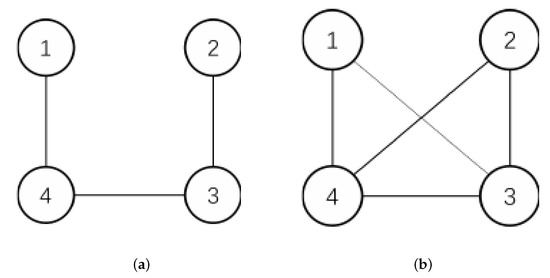  Figure 1. The networkgraph of the examples (a) Network 1, (b) Network 2.
• A fundamental networked game: every pair of players play the game G and G’s payoff bi-matrix is shown in Table 1.
• The SUR F is consisted of $F_1,F_2,F_3$, which are described in (I)–(III), respectively.

Table 1. Payoff bi-matrix of Example 1.

${\mathit{c}}_1\setminus {\mathit{c}}_2$	${\mathit{a}}_1$	${\mathit{a}}_2$
$a_1$	(1, 1)	(0, 1)
$a_2$	(1, 0)	(2, 2)

Table 1. Payoff bi-matrix of Example 1.

${\mathit{c}}_1\setminus {\mathit{c}}_2$	${\mathit{a}}_1$	${\mathit{a}}_2$
$a_1$	(1, 1)	(0, 1)
$a_2$	(1, 0)	(2, 2)

It’s easy to obtain that the adjacent matrices for the graph in Figure 1a is

$$A=\left[\begin{array}{cccc}0& 0& 0& 1\\ 0& 0& 1& 0\\ 0& 1& 0& 1\\ 1& 0& 1& 0\end{array}\right],$$

The payoff matrix is

$$C=\left[\begin{array}{cc}1& 0\\ 1& 2\end{array}\right].$$

Assume the probability of the three SURs are $\alpha =0.3,\beta =0.4,\gamma =0.3$ and the initial strategy profile $x\left(0\right)={\delta }_2[1,2,1,2]$.

First, we establish the dynamics of the game. According to (13) and (19), we can establish the algebraic form of each players’ payoff functions $R_i^{\prime }$ by identifying $a_i\sim {\delta }_2^i,i=1,2$ as follows:

$$\begin{array}{cc}\hfill R_1^{\prime }=& [102-1]W_{[3,3]}\left[0001\right]L\left[\begin{array}{c}0.3\\ 0.4\\ 0.3\end{array}\right]\hfill \\ \hfill =& [\underline{1}1⋮0.7\underline{1.3}⋮0.7\underline{1.3}⋮0.4\underline{1.6}⋮\underline{1}1⋮0.7\underline{1.3}⋮0.7\underline{1.3}⋮0.4\underline{1.6}⋮\hfill \\ \hfill & 0.3\underline{1.7}⋮0\underline{2}⋮0.3\underline{1.7}⋮0\underline{2}⋮0.3\underline{1.7}⋮0\underline{2}⋮0.3\underline{1.7}⋮0\underline{2}],\hfill \\ \hfill R_2^{\prime }=& [102-1]W_{[3,3]}\left[0010\right]L\left[\begin{array}{c}0.3\\ 0.4\\ 0.3\end{array}\right]\hfill \\ \hfill =& [\underline{1}1⋮0.7\underline{1.3}⋮0.7\underline{1.3}⋮0.4\underline{1.6}⋮0.3\underline{1.7}⋮0.3\underline{1.7}⋮0\underline{2}⋮0\underline{2}⋮\hfill \\ \hfill & \underline{1}1⋮0.7\underline{1.3}⋮0.7\underline{1.3}⋮0.4\underline{1.6}⋮0.3\underline{1.7}⋮0.3\underline{1.7}⋮0\underline{2}⋮0\underline{2}],\hfill \\ \hfill R_3^{\prime }=& [102-1]W_{[3,3]}\left[0101\right]L\left[\begin{array}{c}0.3\\ 0.4\\ 0.3\end{array}\right]\hfill \\ \hfill =& [\underline{2}2⋮1.7\underline{2.3}⋮1.4\underline{2.6}⋮1.1\underline{2.9}⋮1.7\underline{2.3}⋮1.4\underline{2.6}⋮1.1\underline{2.9}⋮0.8\underline{3.2}⋮0.9\underline{3.1}⋮\hfill \\ \hfill & 0.6\underline{3.4}⋮0.6\underline{3.4}⋮0.3\underline{3.7}⋮0.6\underline{3.4}⋮0.3\underline{3.7}⋮0.3\underline{3.7}⋮0\underline{4}],\hfill \\ \hfill R_4^{\prime }=& [102-1]W_{[3,3]}\left[1010\right]L\left[\begin{array}{c}0.3\\ 0.4\\ 0.3\end{array}\right]\hfill \\ \hfill =& [\underline{2}2⋮1.4\underline{2.6}⋮1.7\underline{2.3}⋮1.1\underline{2.9}⋮1.3\underline{2.7}⋮1\underline{3}⋮1\underline{3}⋮0.7\underline{3.3}⋮1.3\underline{2.7}⋮\hfill \\ \hfill & 0.7\underline{3.3}⋮1\underline{3}⋮0.4\underline{3.6}⋮0.6\underline{3.4}⋮0.3\underline{3.7}⋮0.3\underline{3.7}⋮0\underline{4}].\hfill \end{array}$$

(39)

Divide $R_i^{\prime }$ into 16 equal blocks and underline the largest column for each block. Then, we obtain

$$\begin{array}{cc}\hfill T_1& ={\delta }_2\left[1222122222222222\right],\hfill \\ \hfill T_2& ={\delta }_2\left[1222122222222222\right],\hfill \\ \hfill T_3& ={\delta }_2\left[1222122222222222\right],\hfill \\ \hfill T_4& ={\delta }_2\left[1222122222222222\right].\hfill \end{array}$$

By multiplying these equations, the state transformation matrix T can be deduced as

$$T={\delta }_{16}\left[116161681616161216161616161616\right].$$

Thus, the algebraic form of the game dynamic is given by

$$x(t+1)=Tx\left(t\right).$$

(40)

Second, with the payoff Function (39), we calculate the matrix $\mathcal{D}$ to seek the NEs. A straightforward calculation of Equation (30) gives that

$$\mathcal{D}=\left[\begin{array}{c}0000-0.6-0.60.60.6-0.6-0.60.60.6-1.2-1.21.21.2\\ 0000-0.6-0.60.60.6-0.6-0.60.60.6-1.2-1.21.21.2\\ 0000-0.6-0.60.60.6-0.6-0.60.60.6-1.2-1.21.21.2\\ 0000-0.6-0.60.60.6-0.6-0.60.60.6-1.2-1.21.21.2\end{array}\right]$$

(41)

By Theorem 1, it is easy to check that $Co{l}_{1,2,3,4,7,8,11,12,15,16}\left(\mathcal{D}\right)\ge 0$. Then, we obtain all the NEs of the game, which are $\{{\delta }_{16}^1,{\delta }_{16}^2,{\delta }_{16}^3,{\delta }_{16}^4,{\delta }_{16}^7,{\delta }_{16}^8,{\delta }_{16}^{11},{\delta }_{16}^{12},{\delta }_{16}^{15},{\delta }_{16}^{16}\}$.

Since the initial strategy is ${\delta }_2^1{\delta }_2^2{\delta }_2^1{\delta }_2^2={\delta }_{16}^6$, by Lemma 3 and by calculating the transformation matrix T, we can obtain that $Co{l}_6\left(T^1\right)={\delta }_{16}^{16}$, which means that the game dynamics will achieve the best profile in the next step by Theorem 2. We can figure out that the best strategy profile is also a NE.

Example 2.

Consider the same problem as in Example 1, but with the payoff matrix shown in Table 2 and the networks in Figure 1a,b. Assume the initial strategy profile $x\left(0\right)={\delta }_2[1,1,1,2]$. Similar to Example 1, we can obtain that the matrix $\mathcal{D}$ for both graphs are

$$\begin{array}{cc}\hfill {\mathcal{D}}^1=& \left[\begin{array}{c}-0.40.40.4-0.40.21-0.2-1-1-0.210.2-0.40.40.4-0.4\\ -0.40.40.4-0.40.21-0.2-1-1-0.210.2-0.40.40.4-0.4\\ -0.40.40.4-0.40.21-0.2-1-1-0.210.2-0.40.40.4-0.4\\ -0.40.40.4-0.40.21-0.2-1-1-0.210.2-0.40.40.4-0.4\end{array}\right],\hfill \\ \hfill {\mathcal{D}}^2=& \left[\begin{array}{c}-1.2-0.61.20.6-0.6-0.60.60.611-1-110.4-1-0.4\\ -1.2-0.61.20.6-0.6-0.60.60.611-1-110.4-1-0.4\\ -1.2-0.61.20.6-0.6-0.60.60.611-1-110.4-1-0.4\\ -1.2-0.61.20.6-0.6-0.60.60.611-1-110.4-1-0.4\end{array}\right].\hfill \end{array}$$

Table 2. Payoff bi-matrix of Example 2.

${\mathit{c}}_1\setminus {\mathit{c}}_2$	${\mathit{a}}_1$	${\mathit{a}}_2$
$a_1$	(1, 1)	(0, 2)
$a_2$	(2, 0)	(−1, −1)

Then, the Nash equilibrium of the NEG under two different networks are $\{{\delta }_{16}^2,{\delta }_{16}^3,{\delta }_{16}^5,{\delta }_{16}^6,{\delta }_{16}^{11},{\delta }_{16}^{12},{\delta }_{16}^{14},{\delta }_{16}^{15}\}$ and $\{{\delta }_{16}^3,{\delta }_{16}^4,{\delta }_{16}^7,{\delta }_{16}^8,{\delta }_{16}^9,{\delta }_{16}^{10},{\delta }_{16}^{13},{\delta }_{16}^{14}\}$, respectively.

It is clear that the corresponding Nash Equilibria of various network structures are not always the same. Calculate the state transformation matrix as follows:

$$\begin{array}{cc}\hfill T^1& ={\delta }_{16}\left[1681216661121514111513591\right],\hfill \\ \hfill T^2& ={\delta }_{16}\left[161613161677101011141611\right],\hfill \end{array}$$

We can obtain the evolution processes under two cases, that is

$$\begin{array}{c}\hfill x^1\left(0\right)={\delta }_{16}^2,x^1\left(1\right)={\delta }_{16}^8,x^1\left(2\right)={\delta }_{16}^2,x^1\left(3\right)={\delta }_{16}^8,\dots \\ \hfill x^2\left(0\right)={\delta }_{16}^2,x^2\left(1\right)={\delta }_{16}^{16},x^2\left(2\right)={\delta }_{16}^1,x^2\left(3\right)={\delta }_{16}^{16},\dots ,\end{array}$$

It is obvious that these two processes will never converge to a fixed point.

Remark 8.

From the evolution process for the Case 1, we can observe, despite the fact that strategy profile ${\delta }_{16}^2$ is a Nash equilibrium, the players’ strategies still change, which is due to the bounded rationality.

Remark 9.

According to those examples, we can know that if the initial strategy is set, we can establish the game evolutionary algebraic expression. In addition, we can know whether the strategy is a NE or best strategy profile by Theorem 1.

5. Conclusions

In this paper, a networked evolutionary game with a mixed strategy updating rules was investigated. By using the STP method, we obtained the algebraic forms of the payoff function and dynamics of the game. Furthermore, a necessary and sufficient condition for the existence of Nash Equilibrium was studied, and an algorithm was given for the seeking of Nash Equilibrium in the pure strategy situation. Based on the algebraic form, the dynamic behavior and the strategy consensus problem of the game have been discussed. Finally, we provide some examples, which are different in the payoff bi-matrices for the game to illustrate our method. However, because of the computational complexity, this method can only be used for small-size NEGs. More broad social dilemma games with multiple populations, such as the Prisoner’s Dilemma, will be taken into consideration for analysis and control issues in future work.

References

- Neumann, J.V.; Morgenstern, O. Theory of Game and Economic Behavior; Princeton University Press: Princeton, NJ, USA, 1944. [Google Scholar]
- Smith, J.M.; Price, G.R. The Logic of Animal Conflict. Nature 1973, 246, 15–18. [Google Scholar] [CrossRef]
- Sun, S.; Yang, H.; Yang, G.; Pi, J. Evolutionary Games and Dynamics in Public Goods Supply with Repetitive Actions. Mathematics 2021, 9, 1726. [Google Scholar] [CrossRef]
- Greene, R.B.; Axelrod, R. The Evolution of Cooperation. J. Policy Anal. Manag. 1984, 4, 140. [Google Scholar] [CrossRef]
- Arefin, M.R.; Kabir, K.M.A.; Jusup, M.; Ito, H.; Tanimoto, J. Social Efficiency Deficit Deciphers Social Dilemmas. Sci. Rep. 2020, 10, 16092. [Google Scholar] [CrossRef]
- Gómez-Gardeñes, J.; Romance, M.; Criado, R.; Vilone, D.; Sánchez, A. Evolutionary Games Defined at the Network Mesoscale: The Public Goods Game. Chaos 2011, 21, 016113. [Google Scholar] [CrossRef]
- Zimmermann, M.G.; Eguíluz, V.M. Cooperation, Social Networks, and the Emergence of Leadership in a Prisoner’s Dilemma with Adaptive Local Interactions. Phys. Rev. E 2005, 056118, 1515. [Google Scholar] [CrossRef]
- Nowak, M.A.; May, R.M. Evolutionary Games and Spatial Chaos. Nature 1992, 359, 826–829. [Google Scholar] [CrossRef]
- Seikh, M.R.; Karmakar, S.; Castillo, O. A Novel Defuzzification Approach of Type-2 Fuzzy Variable to Solving Matrix Games: An Application to Plastic Ban Problem. Iran. J. Fuzzy Syst. 2021, 18, 6262. [Google Scholar] [CrossRef]
- Tanimoto, J. Sociophysics Approach to Epidemics; Evolutionary Economics and Social Complexity Science; Springer: Singapore, 2021; pp. 13–60. [Google Scholar]
- Zhang, J.; Chen, X.; Zhang, C.; Wang, L.; Chu, T. Elimination Mechanism Promotes Cooperation in Coevolutionary Prisoner’s Dilemma Games. Phys. A 2010, 389, 4081–4086. [Google Scholar] [CrossRef]
- Li, R.-H.; Yu, J.X.; Lin, J. Evolution of Cooperation in Spatial Traveler’s Dilemma Game. PLoS ONE 2013, 8, e58597. [Google Scholar] [CrossRef]
- Li, Z.; Cheng, D. Algebraic Approach to Dynamics of Multivalued Networks. Int. J. Bifurc. Chaos 2010, 20, 561–582. [Google Scholar] [CrossRef]
- Cheng, D.; Qi, H. A Linear Representation of Dynamics of Boolean Networks. IEEE Trans. Autom. Contr. 2010, 55, 2251–2258. [Google Scholar] [CrossRef]
- Cheng, D.-Z.; Qi, H.-S.; Zhao, Y. Analysis and Control of Boolean Networks: A Semi-Tensor Product Approach. ACTA Autom. Sin. 2011, 37, 529–540. [Google Scholar] [CrossRef]
- Cheng, D.; Xu, T.; Qi, H. Evolutionarily Stable Strategy of Networked Evolutionary Games. IEEE Trans. Neural Netw. Learn. Syst. 2014, 25, 1335–1345. [Google Scholar] [CrossRef]
- Cheng, D.; He, F.; Qi, H.; Xu, T. Modeling, Analysis and Control of Networked Evolutionary Games. IEEE Trans. Autom. Control 2015, 60, 2402–2415. [Google Scholar] [CrossRef]
- Young, H. The Evolution of Conventions. Econometrica 1993, 61, 57–84. [Google Scholar] [CrossRef]
- Szabó, G.; Tőke, C. Evolutionary Prisoner’s Dilemma Game on a Square Lattice. Phys. Rev. E 1998, 58, 69–73. [Google Scholar] [CrossRef]
- Guo, P.; Wang, Y.; Li, H. Algebraic Formulation and Strategy Optimization for a Class of Evolutionary Networked Games via Semi-Tensor Product Method. Automatica 2013, 49, 3384–3389. [Google Scholar] [CrossRef]
- Zhu, R.; Chen, Z.; Zhang, J.; Liu, Z. Strategy Optimization of Weighted Networked Evolutionary Games with Switched Topologies and Threshold. Knowl.-Based Syst. 2022, 235, 107644. [Google Scholar] [CrossRef]
- Zhao, G.; Wang, Y. Formulation and Optimization Control of a Class of Networked Evolutionary Games with Switched Topologies. Nonlinear Anal.-Hybrid Syst. 2016, 22, 98–107. [Google Scholar] [CrossRef]
- Wang, X.-J.; Gu, C.-L.; Lv, S.-J.; Quan, J. Evolutionary Game Dynamics of Combining the Moran and Imitation Processes. Chin. Phys. B 2019, 28, 20203. [Google Scholar] [CrossRef]
- Zhang, W.; Li, Y.-S.; Xu, C. Co-Operation and Phase Behavior under the Mixed Updating Rules. Chin. Phys. Lett. 2015, 32, 118901. [Google Scholar] [CrossRef]
- Gibbons, R. A Primer in Game Theory; Harvester Wheatheaf: Munich, Germany, 1992; p. 8. ISBN 978-0-7450-1159-2. [Google Scholar]
Publisher’s Note: MDPI stays neutral with regard to jurisdictional claims in published maps and institutional affiliations. |
© 2022 by the authors. Licensee MDPI, Basel, Switzerland. This article is an open access article distributed under the terms and conditions of the Creative Commons Attribution (CC BY) license (https://creativecommons.org/licenses/by/4.0/).