Improved Confidence Interval and Hypothesis Testing for the Ratio of the Coefficients of Variation of Two Uncorrelated Populations

Abstract

One of the most accessible and useful statistical tools for comparing independent populations in different research areas is the coefficient of variation (CV). In this study, first, the asymptotic distribution of the ratio of CV of two uncorrelated populations is investigated. Then, the outputs are used to create a confidence interval and to establish a test of hypothesis about the CV ratio of the populations. The proposed approach is compared with an alternative method, showing its superiority and effectiveness.

1. Introduction

According to the literature, three fundamental measures are used to explain a dataset (random variable). These include central, shape and dispersion tendencies. By obtaining the value of the central tendency, we can know how a random variable is gathered around a central value. The mean, median and mode are the most used criteria to express the central tendency’s measures. Criteria such as range, variance and standard deviation can be used to measure the dispersion of a random variable. In some literature, this is called the random variable distribution scale. Another need of statisticians is to know how a random variable is distributed, or to know its pattern shape, which can be addressed by the use of statistical measures such as kurtosis or skewness.

The coefficient of variation (CV) is obtained by dividing the population standard deviation by the population mean, CV = σ/μ, being an applicable and suitable statistic for evaluating relative variability. The CV is a free parameter that is used in many areas, such as agronomy, biology, engineering, finance, medicine and others, as an indicator of reliability or variability [1,2,3]. In many cases, relating standard deviation to the level of measurement is of great importance to researchers. For this reason, the CV is widely used to measure dispersion. When studying several independent populations, knowing how their CVs are compared is essential. This becomes even more important when populations have skewed distributions. In practical matters, statisticians may be interested in comparing two independent populations’ CV to better understand the data structure. In situations where the means or variances of independent populations are equal, the analysis of variance and Levene’s tests are employed to examine the equality of CVs. If each population has a different mean and variance, it is clearly possible that their CVs are equal. There have been many studies comparing two or more CVs, which we will discuss below. When two CVs are small, the differences between them are likely to be minor, and these minor potential differences can lead to inability to make powerful or definite conclusions. Therefore, the CV ratio is more accurate than the CV difference.

The probability ratio test was introduced by Bennett [4], and later modified by Schaefer and Sullivan [5]. Scientists such as Doornbos et al. [6] and Hedges et al. [7] proposed tests that relied on decentralized meta-analysis. In [8,9,10], some methods were introduced which are known as Wald tests. Pardo and Pardo [11] were able to propose a new method for comparing CVs based on the Rényi divergence. Some researchers, such as Nairy and Rao [12], investigated the inverse CV. Another method proposed for likelihood ratio testing is based on Newton one-step estimators, performed by Verrill and Johnson [13]. The parametric bootstrap (PB) approach was also considered by Jafari and Kazemi [14]. Other statisticians continued these studies and were able to improve them for symmetric distributions, as presented in [15,16,17,18,19,20,21,22,23]. However, comparing two CVs and, in more complex cases, multiple CVs is challenging in practice [24,25]. The approximate interval for the ratio of two CVs in the lognormal distribution was obtained by Nam and Kwon [25]. They obtained the estimate using the Fieller-type log method of variance estimates recovery (MOVER) and the Wald-type method. Two other researchers, Jiang and Wong [26], used the Barlett’s modified likelihood ratio simulation method to make inferences about the ratio of two CVs in the lognormal distribution.

There are many phenomena in the real world that have symmetrical distributions. Due to this reason, most previous studies have focused just on a special type of distributions, especially on the normal distribution. Yue and Baleanu [27] inferred about the CV ratio of two independent symmetric or asymmetric distributions. They studied the asymptotic distribution for the ratio of two populations’ CV. Then, the outputs were used to create the confidence interval and to test the hypothesis about the ratio of CV of the populations.

In this paper, we adopt a procedure similar to those employed in other studies [28,29,30,31,32] to improve the method given by Yue and Baleanu [27]. The rational estimation for the ratio of CV of two populations given by Yue and Baleanu is considered and its asymptotic distribution is investigated. In computing the asymptotic variance, a formulation different from that given by Yue and Baleanu [27] is proposed. Then, using the asymptotic distribution of the given estimator, the confidence interval and hypothesis testing about the ratio of CV of two populations are studied. The new formulation leads to a more powerful estimator and a more accurate confidence interval than those in [27].

The paper is organized as follows: In Section 2, first, a rational estimation for the ratio of CV of two populations is given. Then, the asymptotic distribution of this estimator is considered. Finally, using the asymptotic distribution of the given estimator, the confidence interval and hypothesis testing about the ratio of CV of two populations are studied. In Section 3, various simulated datasets are reviewed and analyzed to verify the accuracy of the theoretical findings. The applicability of the proposed technique in real situations is studied in Section 4. Additionally, Section 5 includes the concluding remarks.

2. Materials and Methods

2.1. Asymptotic Outcomes

Let us consider two uncorrelated variables $X$ and $Y$, with non-zero means of ${\mu }_X$ and ${\mu }_Y$. Their finite $i\mathrm{th}$ central moments are, respectively:

$${\mu }_{iX}=E{(X-{\mu }_X)}^i, {\mu }_{iY}=E{(Y-{\mu }_Y)}^i, i\in \left\{2,3,4\right\}.$$

Furthermore, suppose that $X_1,\dots ,X_m$ and $Y_1,\dots ,Y_n$ are samples that are identically and independently distributed from $X$ and $Y$, respectively. According to what was mentioned in Section 1, given that $C{V}_X$ and $C{V}_Y$ are the CV of $X$ and $Y$, respectively, the parameter

$$\gamma =\frac{C{V}_Y}{C{V}_X}$$

is compelling for statistical inference.

Suppose that

$$m_{iX}=\frac{1}{m}{\sum }_{k=1}^m{\left(x_k-\overline{x}\right)}^i, m_{iY}=\frac{1}{n}{\sum }_{k=1}^n{\left(y_k-\overline{y}\right)}^i, i\in \left\{2,3,4\right\},$$

then, $C{V}_X$ and $C{V}_Y$ are consistently estimated [27,33] by ${\widehat{CV}}_X=\frac{\sqrt{m_{2X}}}{\overline{X}}$ and ${\widehat{CV}}_Y=\frac{\sqrt{m_{2Y}}}{\overline{Y}}$, respectively. Therefore, it follows that

$$\widehat{\gamma }=\frac{{\widehat{CV}}_Y}{{\widehat{CV}}_X}$$

has the ability to estimate the parameter $\gamma$ reasonably. For convenience,$n=m$ can be defined. At $n\ne m,$ $n^{*}=min\left(m,n\right)$ can be used instead of m and n.

Lemma 1.

If the mentioned assumptions are accepted, thus

$$\sqrt{n}\left({\widehat{CV}}_X-C{V}_X\right)\stackrel{L}{\to }N\left(0,{\delta }_X^2\right), as n\to \infty ,$$

where

$${\delta }_X^2=\left[\frac{{\mu }_{4X}-{\mu }_{2X}^2}{4{\mu }_X^2{\mu }_{2X}}-\frac{{\mu }_{3X}}{{\mu }_X^3}+\frac{{\mu }_{2X}^2}{{\mu }_{4X}}\right]$$

represents the asymptotic variance.

Proof. 

The proof sketch is given in [33]. □

In the subsequent theorem, Yue and Baleanu [33] used the asymptotic distribution of $\widehat{\gamma }$ to build the confidence interval and test the hypothesis about γ.

Lemma 2.

If the previous assumptions are accepted, thus

$$\sqrt{n}\left(\widehat{\gamma }-\gamma \right)\stackrel{\mathcal{L}}{\to }N\left(0,{\lambda }^2\right), as n\to \infty ,$$

where

$${\lambda }^2=\frac{1}{C{V}_X^2}\left({\gamma }^2{\delta }_X^2+{\delta }_Y^2\right),$$

and

$${\delta }_Y^2=\left[\frac{{\mu }_{4Y}-{\mu }_{2Y}^2}{4{\mu }_Y^2{\mu }_{2Y}}-\frac{{\mu }_{3Y}}{{\mu }_Y^3}+\frac{{\mu }_{2Y}^2}{{\mu }_{4Y}}\right].$$

Proof of Lemma 2.

The proof sketch is given in [27]. □

It can be observed that the asymptotic variance ${\lambda }^2$ depends on the unknown parameters $C{V}_X$, ${\delta }_X^2$, ${\delta }_Y^2$ and γ. Yue and Baleanu [33] estimated ${\lambda }^2$ by

$${\widehat{\lambda }}^2=\frac{1}{\widehat{C}{V}_X^2}\left({\widehat{\gamma }}^2{\widehat{\delta }}_X^2+{\widehat{\delta }}_Y^2\right),$$

where

$${\widehat{\delta }}_X^2=\left[\frac{m_{4X}-m_{2X}^2}{4{\overline{X}}^2{m}_{2X}}-\frac{m_{3X}}{{\overline{X}}^3}+\frac{m_{2X}^2}{m_{4X}}\right],$$

and

$${\widehat{\delta }}_Y^2=\left[\frac{m_{4Y}-m_{2Y}^2}{4{\overline{Y}}^2{m}_{2Y}}-\frac{m_{3Y}}{{\overline{Y}}^3}+\frac{m_{2Y}^2}{m_{4Y}}\right].$$

They used Slutsky’s theorem and proved that $\widehat{\lambda }\stackrel{p}{\to }\lambda ,$ as $n\to \infty$.

In this work, we rewrite the asymptotic variance ${\lambda }^2$ in an alternative form and re-estimate it using a more robust estimator. The asymptotic variance ${\lambda }^2$ can be represented by

$${\lambda }^2=\frac{1}{{\gamma }^2}\left({\left(\frac{{\delta }_X}{C{V}_X}\right)}^2+{\left(\frac{{\delta }_Y}{C{V}_Y}\right)}^2\right).$$

Therefore, we can construct the asymptotic distribution as

$$T_n=\sqrt{n}\left(\frac{\widehat{\gamma }-\gamma }{\lambda }\right)=\sqrt{n}{\left({\left(\frac{{\delta }_X}{C{V}_X}\right)}^2+{\left(\frac{{\delta }_Y}{C{V}_Y}\right)}^2\right)}^{-1/2}\left(\frac{\widehat{\gamma }}{\gamma }-1\right)\stackrel{\mathcal{L}}{\to }N\left(0,1\right), as n\to \infty .$$

Theorem 1.

If the previous assumptions are accepted, thus

$$T_n^{*}=\sqrt{n}\left(\frac{\widehat{\gamma }-\gamma }{{\widehat{\lambda }}_{opt}}\right)\stackrel{\mathcal{L}}{\to }N\left(0,1\right), as n\to \infty ,$$

where

$${\widehat{\lambda }}_{opt}^2=\frac{1}{{\widehat{\gamma }}^2}\left({\left(\frac{S_X}{{\widehat{CV}}_X}\right)}^2+{\left(\frac{S_Y}{{\widehat{CV}}_Y}\right)}^2\right).$$

Proof of Theorem 1.

Due to the weak law of large numbers, it is clear that

$$\overline{X}\stackrel{p}{\to }{\mu }_X, \overline{Y}\stackrel{p}{\to }{\mu }_Y, m_{iX}\stackrel{p}{\to }{\mu }_{iX}, m_{iY}\stackrel{p}{\to }{\mu }_{iY}, i\in \left\{2,3,4\right\},$$

as $n\to \infty .$ □

As a result, by using Slutsky’s theorem, we know that ${\widehat{\lambda }}_{opt}\stackrel{p}{\to }\lambda ,$ as $n\to \infty$. With the help of Lemma 2 the proof is completed.

2.1.1. Building the Confidence Interval

To construct an asymptotic confidence interval for γ, we need a pivotal quantity for the parameter γ. Based on the previous results, T is a pivotal quantity for γ. Therefore, T can be used for this purpose, as follows:

$$\left(\frac{\widehat{\gamma }}{1+\frac{Z_{\alpha /2}}{\sqrt{n}}{\left({\left(\frac{S_X}{{\widehat{CV}}_X}\right)}^2+{\left(\frac{S_Y}{{\widehat{CV}}_Y}\right)}^2\right)}^{1/2}},\frac{\widehat{\gamma }}{1-\frac{Z_{\alpha /2}}{\sqrt{n}}{\left({\left(\frac{S_X}{{\widehat{CV}}_X}\right)}^2+{\left(\frac{S_Y}{{\widehat{CV}}_Y}\right)}^2\right)}^{1/2}}\right).$$

2.1.2. Hypothesis Testing

In practical situations, scientists need to test the parameter γ. As a particular instance, the null hypothesis ${\mathrm{H}}_0:\gamma =1$ shows that the CVs are the same in both populations. To accomplish the hypothesis test ${\mathrm{H}}_0$: γ =${\gamma }_0$, the test statistic

$$T_0=\sqrt{n}{\left({\left(\frac{S_X}{{\widehat{CV}}_X}\right)}^2+{\left(\frac{S_Y}{{\widehat{CV}}_Y}\right)}^2\right)}^{-\frac{1}{2}}\left(\frac{\widehat{\gamma }}{{\gamma }_0}-1\right)$$

can be generally applied.

If the null hypothesis ${\mathrm{H}}_0: \gamma ={\gamma }_0$ is verified, thus the asymptotic distribution of $T_0$ is standard normal.

It should be noted that this method can be used for all distributions, because asymptotic methods have been used and the technique includes all exponential or non-exponential distributions. Moreover, the method is also appropriate if the populations have different distributions.

3. Results

3.1. Simulation Study

In this section, various simulated datasets are reviewed and analyzed to verify the accuracy of the theoretical findings. To compare the results obtained with the proposed method and those from the method given by Yue and Baleanu [27], we consider the distributions used therein. To simulate different samples of one symmetric and two asymmetric distributions, populations X and Y are considered. For this purpose, we selected the normal, and the gamma and beta distributions, respectively, with a variety of values of CV, $\left(C{V}_X,C{V}_Y\right)\in \left\{\left(1,1\right),\left(1,2\right),\left(2,3\right),\left(2,5\right)\right\}$, that is, identical to $\gamma \in \left\{1,2,1.5,2.5\right\}$. Figure 1, Figure 2 and Figure 3 depict the probability density function (PDF) for the intended distributions.

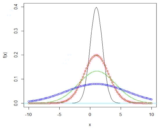
Figure 1. The PDF of the distribution normal (μ, ${\sigma }^2$) for different values of CV (black: CV = 1; red: CV = 2; green: CV = 3; blue: CV = 5).

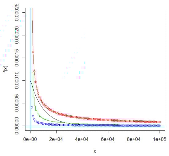
Figure 2. The PDF of the distribution gamma (α, λ) for different values of CV (blue: α = 0.04, λ = 0.001, CV = 5; green: α = 0.11, λ = 0.001, CV = 3; red: α = 0.25, λ = 0.001, CV = 2; black: α = 1, λ = 0.001, CV = 1).

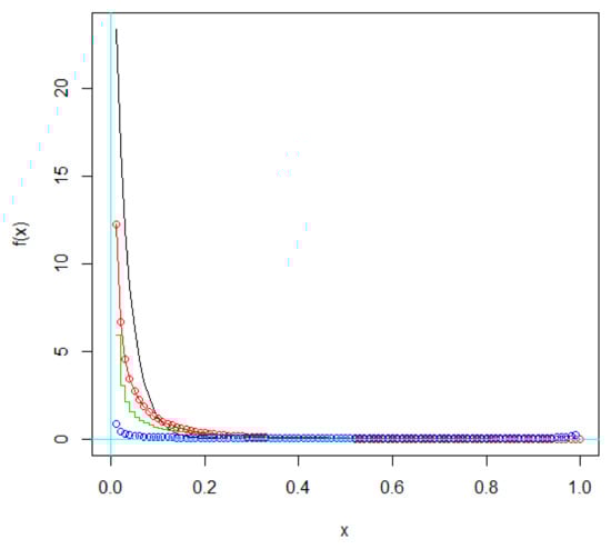
Figure 3. PDF of distribution of beta (α, β) in the presence of different values of CV (blue: α = 0.009, β = 0.285, CV = 5; green: α = 0.08, β = 2.51; red: α = 0.21, β = 6.87, CV = 2; black: α = 0.94, β = 30.39, CV = 1).

The simulations are performed using the software R 3.3.2, adopting 1000 repetitions.

For investigating the accuracy of the proposed method, we compute the coverage probability, by

$$\mathrm{CP}=\frac{\mathrm{number} \mathrm{of} \mathrm{repetitions} \mathrm{where} \mathrm{proposed} \mathrm{confidence} \mathrm{interval} \mathrm{includes} \mathrm{right} \gamma }{1000}.$$

Furthermore, the value of test statistic $T_0$ is calculated. Then, we use the Shapiro–Wilk test to check the normality. After that, Q–Q plots are drawn to confirm the normality assumption for the offered test statistic. Table 1 summarizes the values of CP of the proposed method and those of the method by Yue and Baleanu [27], for various settings of parameters.

Table 1. The values of CP of the proposed and the Yue and Baleanu [27] methods, for various settings of parameters.

			$\left(\mathit{m},\mathit{n}\right)$									Mean Absolute Difference from 0.95
Distribution	$\left(\mathit{C}{\mathit{V}}_{\mathit{X}},\mathit{C}{\mathit{V}}_{\mathit{Y}}\right)$	Method	(50,100)	(75,100)	(100,100)	(100,200)	(200,300)	(500,500)	(500,700)	(700,1000)	(1000,1000)
Normal	$\left(1,1\right)$	Proposed	0.947	0.949	0.949	0.949	0.951	0.950	0.949	0.950	0.950	0.001
		Yue and Baleanu	0.945	0.947	0.948	0.951	0.953	0.957	0.959	0.960	0.951	0.005
	$\left(1,2\right)$	Proposed	0.948	0.949	0.949	0.951	0.950	0.950	0.950	0.949	0.951	0.001
		Yue and Baleanu	0.945	0.948	0.948	0.952	0.953	0.953	0.958	0.959	0.952	0.005
	$\left(2,3\right)$	Proposed	0.947	0.948	0.948	0.949	0.950	0.950	0.950	0.950	0.950	0.001
		Yue and Baleanu	0.944	0.948	0.949	0.953	0.953	0.956	0.959	0.961	0.952	0.006
	$\left(2,5\right)$	Proposed	0.947	0.949	0.949	0.950	0.950	0.950	0.951	0.951	0.950	0.001
		Yue and Baleanu	0.946	0.950	0.950	0.950	0.955	0.954	0.956	0.960	0.952	0.004
Gamma	$\left(1,1\right)$	Proposed	0.947	0.950	0.950	0.951	0.950	0.950	0.950	0.950	0.951	0.001
		Yue and Baleanu	0.946	0.948	0.948	0.952	0.956	0.956	0.958	0.961	0.952	0.006
	$\left(1,2\right)$	Proposed	0.946	0.949	0.949	0.951	0.950	0.950	0.950	0.949	0.950	0.001
		Yue and Baleanu	0.947	0.949	0.949	0.951	0.954	0.955	0.958	0.961	0.951	0.005
	$\left(2,3\right)$	Proposed	0.946	0.949	0.950	0.950	0.949	0.950	0.951	0.949	0.950	0.001
		Yue and Baleanu	0.947	0.950	0.950	0.952	0.953	0.956	0.959	0.961	0.952	0.005
	$\left(2,5\right)$	Proposed	0.946	0.948	0.949	0.950	0.951	0.949	0.949	0.949	0.950	0.002
		Yue and Baleanu	0.945	0.949	0.949	0.952	0.956	0.957	0.958	0.962	0.953	0.006
Beta	$\left(1,1\right)$	Proposed	0.947	0.950	0.950	0.950	0.951	0.950	0.950	0.950	0.950	0.001
		Yue and Baleanu	0.944	0.950	0.950	0.950	0.954	0.955	0.958	0.961	0.954	0.005
	$\left(1,2\right)$	Proposed	0.947	0.949	0.949	0.949	0.949	0.950	0.951	0.951	0.949	0.001
		Yue and Baleanu	0.946	0.948	0.949	0.952	0.954	0.956	0.957	0.960	0.953	0.005
	$\left(2,3\right)$	Proposed	0.946	0.949	0.949	0.950	0.950	0.950	0.950	0.950	0.950	0.001
		Yue and Baleanu	0.945	0.947	0.948	0.952	0.954	0.956	0.958	0.959	0.952	0.005
	$\left(2,5\right)$	Proposed	0.948	0.949	0.950	0.950	0.949	0.950	0.951	0.950	0.950	0.001
		Yue and Baleanu	0.945	0.948	0.948	0.951	0.954	0.955	0.956	0.960	0.952	0.005
Mean Absolute Difference from 0.95		Proposed	0.003	0.001	0.002	0.001	0.001	0.001	0.001	0.001	0.002	0.001
		Yue and Baleanu	0.005	0.002	0.003	0.002	0.004	0.002	0.008	0.010	0.004	0.005

3.2. Results

From Table 1, we conclude that both methods have been successful in controlling type I error. However, as can be seen, our method achieved better results.

From Table 2, we verify that the average length of the confidence interval of our method is relatively smaller than the length of the confidence interval of Ballino’s method. Additionally, as the sample size increases, the length of the confidence interval decreases.

Table 2. The values of average lengths of the proposed and the Yue and Baleanu [27] methods, for various settings of parameters.

Distribution	$\left(\mathit{C}{\mathit{V}}_{\mathit{X}},\mathit{C}{\mathit{V}}_{\mathit{Y}}\right)$	Method	$\left(\mathit{m},\mathit{n}\right)$
			(50,100)	(75,100)	(100,100)	(100,200)	(200,300)	(500,500)	(500,700)	(700,1000)	(1000,1000)
Normal	$\left(1,1\right)$	Proposed	0.194	0.173	0.142	0.139	0.114	0.092	0.084	0.073	0.063
		Yue and Baleanu	0.385	0.346	0.303	0.256	0.204	0.198	0.174	0.151	0.135
	$\left(1,2\right)$	Proposed	0.193	0.172	0.159	0.124	0.107	0.099	0.089	0.073	0.063
		Yue and Baleanu	0.366	0.327	0.312	0.265	0.225	0.196	0.171	0.148	0.123
	$\left(2,3\right)$	Proposed	0.185	0.161	0.145	0.136	0.119	0.097	0.086	0.077	0.061
		Yue and Baleanu	0.383	0.336	0.294	0.253	0.231	0.187	0.162	0.153	0.134
	$\left(2,5\right)$	Proposed	0.200	0.170	0.156	0.132	0.115	0.092	0.082	0.071	0.061
		Yue and Baleanu	0.375	0.350	0.291	0.249	0.202	0.195	0.167	0.148	0.124
Gamma	$\left(1,1\right)$	Proposed	0.195	0.175	0.148	0.123	0.112	0.092	0.086	0.073	0.061
		Yue and Baleanu	0.376	0.325	0.280	0.261	0.217	0.181	0.177	0.155	0.133
	$\left(1,2\right)$	Proposed	0.189	0.174	0.146	0.137	0.108	0.096	0.080	0.076	0.069
		Yue and Baleanu	0.398	0.349	0.318	0.245	0.211	0.189	0.166	0.148	0.134
	$\left(2,3\right)$	Proposed	0.188	0.180	0.140	0.124	0.106	0.097	0.081	0.071	0.066
		Yue and Baleanu	0.363	0.321	0.302	0.250	0.211	0.192	0.172	0.147	0.128
	$\left(2,5\right)$	Proposed	0.196	0.175	0.150	0.125	0.105	0.093	0.083	0.074	0.070
		Yue and Baleanu	0.375	0.333	0.291	0.268	0.220	0.197	0.180	0.151	0.137
Beta	$\left(1,1\right)$	Proposed	0.187	0.167	0.145	0.127	0.112	0.091	0.089	0.074	0.068
		Yue and Baleanu	0.360	0.358	0.317	0.279	0.206	0.197	0.166	0.150	0.130
	$\left(1,2\right)$	Proposed	0.190	0.168	0.148	0.138	0.102	0.098	0.081	0.074	0.065
		Yue and Baleanu	0.383	0.359	0.296	0.278	0.211	0.186	0.179	0.147	0.128
	$\left(2,3\right)$	Proposed	0.195	0.166	0.141	0.140	0.104	0.094	0.085	0.072	0.063
		Yue and Baleanu	0.371	0.327	0.312	0.241	0.217	0.188	0.169	0.141	0.140
	$\left(2,5\right)$	Proposed	0.192	0.167	0.144	0.139	0.105	0.096	0.089	0.078	0.063
		Yue and Baleanu	0.373	0.339	0.280	0.264	0.232	0.187	0.170	0.147	0.136

From Table 1, we verify that the CP of the proposed method is close to the intended level (1 − α = 0.95). This is more visible when the sample size increases. As a result, the introduced approach controls type I error. This means that about 95% of the simulated confidence intervals contain true γ, so it is accepted that the proposed confidence is an asymptomatic confidence interval for γ. Moreover, since the CP of the proposed method is closer to the intended level than the one of the alternative method [27], our approach is more robust. Table 3 shows the CPU time needed for running the proposed and the Yue and Baleanu [27] methods, for various combinations of parameters. We verify that our approach is faster than the comparative one.

Table 3. The CPU time needed for running the proposed and the Yue and Baleanu [27] methods, for various settings of parameters.

			$\left(\mathit{m},\mathit{n}\right)$
Distribution	$\left(\mathit{C}{\mathit{V}}_{\mathit{X}},\mathit{C}{\mathit{V}}_{\mathit{Y}}\right)$	Method	$\left(50,100\right)$	$\left(75,100\right)$	$\left(100,200\right)$	$\left(200,300\right)$	$\left(500,700\right)$	$\left(700,1000\right)$
Normal	$\left(1,1\right)$	Proposed	7.00	8.00	9.00	16.00	43.00	57.00
		Yue and Baleanu	8.64	10.08	140.8	23.09	51.92	68.67
	$\left(1,2\right)$.	Proposed	8.00	8.00	12.00	19.00	21.00	48.00
		Yue and Baleanu	8.72	10.29	16.41	21.58	52.19	74.17
	$\left(2,3\right)$	Proposed	8.00	8.00	10.00	15.00	38.00	62.00
		Yue and Baleanu	9.52	9.50	142	21.10	51.05	65.87
	$\left(2,5\right)$	Proposed	7.00	8.00	11.00	19.00	26.00	61.00
		Yue and Baleanu	9.35	10.90	15.25	24.31	49.97	74.90
Gamma	$\left(1,1\right)$	Proposed	8.00	9.00	11.00	16.00	26.00	58.00
		Yue and Baleanu	9.45	9.02	15.16	22.13	47.05	74.92
	$\left(1,2\right)$	Proposed	8.00	9.00	12.00	20.00	27.00	65.00
		Yue and Baleanu	8.00	9.58	14.65	24.87	49.96	66.20
	$\left(2,3\right)$	Proposed	7.00	8.00	11.00	17.00	23.00	52.00
		Yue and Baleanu	9.63	9.29	14.47	21.91	52.52	66.84
	$\left(2,5\right)$	Proposed	7.00	8.00	9.00	17.00	28.00	50.00
		Yue and Baleanu	8.69	9.83	16.29	24.27	50.68	66.11
Beta	$\left(1,1\right)$	Proposed	8.00	9.00	11.00	20.00	43.00	49.00
		Yue and Baleanu	9.53	10.57	14.19	21.47	53.26	66.58
	$\left(1,2\right)$	Proposed	7.00	9.00	12.00	15.00	42.00	57.00
		Yue and Baleanu	9.20	9.50	14.15	24.85	48.67	75.00
	$\left(2,3\right)$	Proposed	7.00	8.00	12.00	17.00	37.00	55.00
		Yue and Baleanu	9.02	9.63	14.25	23.52	50.29	69.67
	$\left(2,5\right)$	Proposed	7.00	8.00	9.00	15.00	22.00	63.00
		Yue and Baleanu	8.75	9.17	15.73	22.89	50.79	73.95

Table 4 summarizes the p-values for assessing the normality of the statistic T₀. We verify that all p-values are greater than 0.05, meaning that the normality of the introduced statistical test is confirmed by the Shapiro–Wilk test. This is also confirmed in the Q–Q plots depicted in Figure 4. Indeed, the points are around the direct line, so the observed values (quantiles) are very much like the quantiles of the normal distribution. Accordingly, the simulation outcomes verified that the asymptotic theoretical findings seem to be satisfied towards a parameter setting. As a result, our method is a suitable selection to perform a test hypothesis and build a confidence interval for the CV ratio of two independent populations.

Table 4. The p-values to investigate the normality of the statistic $T_0$.

		$\left(\mathit{m},\mathit{n}\right)$
Distribution	$\left(\mathit{C}{\mathit{V}}_{\mathit{X}},\mathit{C}{\mathit{V}}_{\mathit{Y}}\right)$	(50,100)	(75,100)	(100,100)	(100,200)	(200,300)	(500,500)	(500,700)	(700,1000)	(1000,1000)
Normal	$\left(1,1\right)$	$0.061$	$0.165$	0.849	$0.541$	$0.885$	0.863	$0.875$	$0.886$	0.861
	$\left(1,2\right)$	$0.605$	$0.224$	0.871	$0.559$	$0.892$	0.861	$0.895$	$0.901$	0.870
	$\left(2,3\right)$	$0.112$	$0.104$	0.845	$0.891$	$0.903$	0.895	$0.874$	$0.896$	0.887
	$\left(2,5\right)$	$0.099$	$0.163$	0.855	$0.435$	$0.898$	0.858	$0.895$	$0.890$	0.844
Gamma	$\left(1,1\right)$	$0.130$	$0.236$	0.564	$0.905$	$0.885$	0.845	$0.896$	$0.903$	0.853
	$\left(1,2\right)$	$0.119$	$0.099$	0.590	$0.892$	$0.808$	0.851	$0.884$	$0,981$	0.845
	$\left(2,3\right)$	$0.120$	$0.231$	0.866	$0.900$	$0.903$	0.863	$0.896$	$0.871$	0.895
	$\left(2,5\right)$	$0.310$	$0.490$	0.787	$0.902$	$0.908$	0.857	$0.893$	$0.891$	0.866
Beta	$\left(1,1\right)$	$0.079$	$0.410$	0.856	$0.249$	$0.904$	0.863	$0.843$	$0.601$	0.841
	$\left(1,2\right)$	$0.319$	$0.325$	0.864	$0.903$	$0.876$	0.896	$0.815$	$0.877$	0.890
	$\left(2,3\right)$	$0.216$	$0.086$	0.857	$0.853$	$0.891$	0.850	$0.912$	$0.908$	0.866
	$\left(2,5\right)$	$0.106$	$0.286$	0.835	$0.884$	$0.901$	0.874	$0.902$	$0.909$	0.904

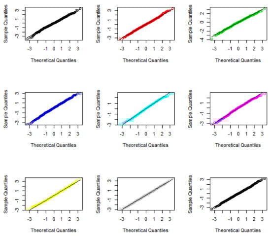
Figure 4. The Q–Q plots used to investigate the normality of the statistic $T_0$. First column: Up: ($C{V}_X$,$C{V}_Y)=\left(1,1\right)$ and $\left(m,n\right)=\left(50,100\right)$; middle: ($C{V}_X$,$C{V}_Y)=\left(1,2\right)$ and $\left(m,n\right)=\left(75,100\right);$ down: ($C{V}_X$,$C{V}_Y)=\left(2,3\right)$ and $\left(m,n\right)=\left(100,100\right)$; Second column: Up: ($C{V}_X$,$C{V}_Y)=\left(1,2\right)$ and $\left(m,n\right)=\left(100,200\right)$; middle: ($C{V}_X$,$C{V}_Y)=\left(2,3\right)$ and $\left(m,n\right)=\left(200,300\right);$ down: ($C{V}_X$,$C{V}_Y)=\left(2,5\right)$ and $\left(m,n\right)=\left(500,500\right)$; Third column: Up: ($C{V}_X$,$C{V}_Y)=\left(1,1\right)$ and $\left(m,n\right)=\left(500,700\right)$; middle: ($C{V}_X$,$C{V}_Y)=\left(1,2\right)$ and $\left(m,n\right)=\left(700,1000\right)$; down: ($C{V}_X$,$C{V}_Y)=\left(2,5\right)$ and $\left(m,n\right)=\left(1000, 1000\right)$.

As the sample size increases, the power also increases. From Table 5, it can also be seen that our method is more powerful than the one by Yue and Baleanu [27].

Table 5. The values of powers of the proposed and the Yue and Baleanu [27] methods, for various settings of parameters.

Distribution	$\left(\mathit{C}{\mathit{V}}_{\mathit{X}},\mathit{C}{\mathit{V}}_{\mathit{Y}}\right)$	Method	$\left(\mathit{m},\mathit{n}\right)$
			(50,100)	(75,100)	(100,100)	(100,200)	(200,300)	(500,500)	(500,700)	(700,1000)	(1000,1000)
Normal	$\left(1,2\right)$	Proposed	0.814	0.863	0.891	0.909	0.941	0.966	0.983	0.996	0.998
		Yue and Baleanu	0.625	0.655	0.687	0.723	0.753	0.794	0.875	0.917	0.934
	$\left(2,3\right)$	Proposed	0.812	0.845	0.860	0.938	0.946	0.978	0.979	0.996	0.999
		Yue and Baleanu	0.621	0.652	0.705	0.717	0.762	0.824	0.852	0.911	0.934
	$\left(2,5\right)$	Proposed	0.841	0.850	0.875	0.932	0.960	0.971	0.986	1.000	1.000
		Yue and Baleanu	0.619	0.670	0.698	0.714	0.777	0.794	0.845	0.918	0.929
Gamma	$\left(1,2\right)$	Proposed	0.840	0.833	0.871	0.919	0.950	0.967	0.976	0.994	0.998
		Yue and Baleanu	0.601	0.663	0.697	0.736	0.771	0.830	0.851	0.918	0.935
	$\left(2,3\right)$	Proposed	0.844	0.832	0.893	0.935	0.942	0.972	0.981	0.990	0.996
		Yue and Baleanu	0.643	0.679	0.680	0.726	0.752	0.829	0.879	0.903	0.947
	$\left(2,5\right)$	Proposed	0.817	0.843	0.898	0.923	0.948	0.961	0.977	0.990	0.995
		Yue and Baleanu	0.610	0.675	0.683	0.725	0.757	0.817	0.852	0.895	0.934
Beta	$\left(1,2\right)$	Proposed	0.841	0.839	0.896	0.913	0.949	0.971	0.980	0.999	1.000
		Yue and Baleanu	0.648	0.658	0.684	0.731	0.757	0.817	0.858	0.918	0.948
	$\left(2,3\right)$	Proposed	0.803	0.866	0.865	0.924	0.951	0.975	0.984	0.995	0.996
		Yue and Baleanu	0.646	0.667	0.702	0.720	0.751	0.825	0.868	0.915	0.921
	$\left(2,5\right)$	Proposed	0.830	0.875	0.877	0.912	0.950	0.975	0.980	0.996	0.999
		Yue and Baleanu	0.621	0.653	0.694	0.729	0.752	0.806	0.867	0.910	0.938

4. Discussion

4.1. Application

The applicability of the proposed technique in real situations is studied. For this purpose, we analyze a dataset containing two features: The humidity (%) and the scale of mouth, foot and hand disease outbreak from 2010 until 2017 for two regions in Malaysia (Sarawak and Malacca). Details about the datasets can be found in [34,35]. Table 6 and Figure 5 report the descriptive statistics and histograms of the features. The results show that the CVs of the humidity in Sarawak and Malacca are 0.8872 and 1.0788, respectively. The CVs of the disease outbreak in Sarawak and Malacca are 0.0107 and 0.0159, respectively.

Table 6. Descriptive statistics about the humidity and the scale of mouth, foot and hand disease outbreak in Sarawak and Malacca.

Feature	N	Region	Mean	Standard Deviation	CV
Disease outbreak	6220	Malacca	64.719	69.924	1.078
	62061	Sarawak	646.468	573.597	0.887
Humidity (%)	6220	Malacca	75.704	1.185	0.015
	62061	Sarawak	75.150	0.821	0.010

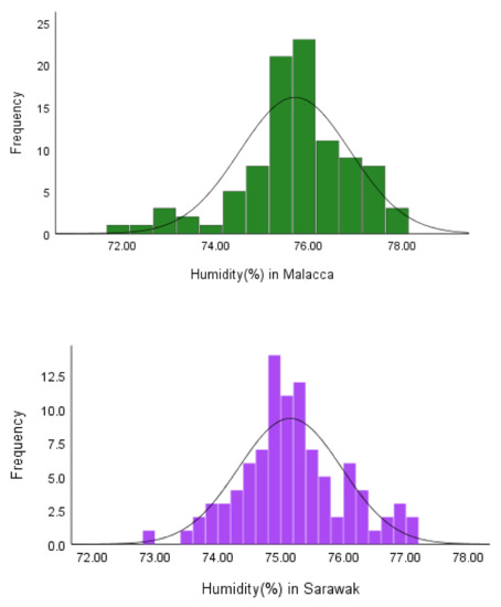
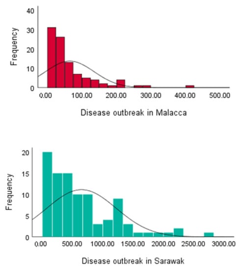
Figure 5. The humidity and the scale of mouth, foot and hand disease outbreak in Sarawak and Malacca.

4.2. Discussion

The proposed approach is applied to provide 95% confidence intervals for the ratio of the CV of the two considered features in Malacca with respect to Sarawak. The computed confidence intervals are reported in Table 7. It can be observed that the intervals (0.973, 1.459) and (1.189, 1.783) are the 95% confidence intervals for the ratio of the CV of the disease outbreak and the ratio of the CV of the humidity in Malacca with respect to Sarawak. Since the lower bound (1.189, 1.783) is greater than 1, it can be concluded that the CV of the humidity in Malacca is significantly higher than the CV of the humidity in Sarawak. Moreover, since the interval (0.973, 1.459) contains the value 1, the hypothesis of the equality of the CV of the disease outbreak in Sarawak and Malacca cannot be rejected.

Table 7. The lower and upper bounds of the computed confidence intervals for the ratio of the CV of the humidity and the ratio of the CV of the scale of hand, foot and mouth disease outbreak in Malacca with respect to Sarawak.

Feature		Ratio	Lower Bound	Upper Bound
Proposed Method	Disease outbreak	1.216	1.122	1.309
	Humidity (%)	1.431	0.571	2.292
Yue and Baleanu’s method	Disease outbreak	1.216	1.078	1.353
	Humidity (%)	1.431	0.253	2.610

It is not necessary that the distribution of x and y be the same, and it is omitted from the article and the table due to length. Therefore, this method can be used when the x and y distributions are different.

As can be seen in Table 7, the confidence interval of our method is slightly smaller than the confidence interval of Yue and Baleanu’s method. This is because we wrote the variance in such a way that not only simplifies the calculations, but also increases the power.

5. Conclusions

To compare populations, the CV is a useful, convenient and simple tool. In countless cases, two populations have the same CV, despite different means and variances. One way to understand the data structure is to study the equality of the two separate populations’ CVs. However, when the difference between the two CVs is slight, it does not provide a solid and valuable interpretation. For this reason, the CV ratio is used, which is more accurate. Asymptotic distribution was proposed in this paper, and then the test of hypothesis and the asymptotic confidence interval for the CV ratio of two independent populations were extracted. The findings showed that the probability of coverage is very close to the desired level when increasing the sample. Based on this, it can be concluded that the introduced methodology controls the type I error. In addition, CPU times confirmed that the proposed method does not involve excessive computational burden. In addition, the normality of the introduced test statistics was confirmed using the normal Shapiro–Wilk test and Q–Q plots. According to the results, it was observed that the asymptotic approximation acted very well for the whole simulated dataset. Moreover, the proposed method is more powerful than the comparative method given by Yue and Baleanu [27].

References

- Meng, Q.; Yan, L.; Chen, Y.; Zhang, Q. Generation of Numerical Models of Anisotropic Columnar Jointed Rock Mass Using Modified Centroidal Voronoi Diagrams. Symmetry 2018, 10, 618. [Google Scholar] [CrossRef]
- Aslam, M.; Aldosari, M.S. Inspection Strategy under Indeterminacy Based on Neutrosophic Coefficient of Variation. Symmetry 2019, 11, 193. [Google Scholar] [CrossRef]
- Iglesias-Caamaño, M.; Carballo-López, J.; Álvarez-Yates, T.; Cuba-Dorado, A.; García-García, O. Intrasession Reliability of the Tests to Determine Lateral Asymmetry and Performance in Volleyball Players. Symmetry 2018, 10, 416. [Google Scholar] [CrossRef]
- Bennett, B.M. On an approximate test for homogeneity of coefficients of variation. In Contribution to Applied Statistics; Ziegler, W.J., Ed.; Birkhauser Verlag: Basel, Switzerland; Stuttgart, Germany, 1976; pp. 169–171. [Google Scholar]
- Shafer, N.J.; Sullivan, J.A. A simulation study of a test for the equality of the coefficients of variation. Commun. Stat. Simul. Comput. 1986, 15, 681–695. [Google Scholar] [CrossRef]
- Doornbos, R.; Dijkstra, J.B. A multi sample test for the equality of coefficients of variation in normal populations. Commun. Stat. Simul. Comput. 1983, 12, 147–158. [Google Scholar] [CrossRef]
- Hedges, L.; Olkin, I. Statistical Methods for Meta-Analysis; Academic Press: Orlando, FL, USA, 1985. [Google Scholar]
- Rao, K.A.; Vidya, R. On the performance of test for coefficient of variation. Calcutta. Stat. Assoc. Bull. 1992, 42, 87–95. [Google Scholar] [CrossRef]
- Gupta, R.C.; Ma, S. Testing the equality of coefficients of variation in k normal populations. Commun. Stat. Theory Methods 1996, 25, 115–132. [Google Scholar] [CrossRef]
- Rao, K.A.; Jose, C.T. Test for equality of coefficient of variation of k populations. In Proceedings of the 53rd Session of International Statistical Institute, Seoul, Korea, 22–29 August 2001. [Google Scholar]
- Pardo, M.C.; Pardo, J.A. Use of Rényi’s divergence to test for the equality of the coefficient of variation. J. Comput. Appl. Math. 2000, 116, 93–104. [Google Scholar] [CrossRef]
- Nairy, K.S.; Rao, K.A. Tests of coefficient of variation of normal population. Commun. Stat. Simul. Comput. 2003, 32, 641–661. [Google Scholar] [CrossRef]
- Verrill, S.; Johnson, R.A. Confidence bounds and hypothesis tests for normal distribution coefficients of variation. Commun. Stat. Theory Methods 2007, 36, 2187–2206. [Google Scholar] [CrossRef]
- Jafari, A.A.; Kazemi, M.R. A parametric bootstrap approach for the equality of coefficients of variation. Comput. Stat. 2013, 28, 2621–2639. [Google Scholar] [CrossRef]
- Feltz, G.J.; Miller, G.E. An asymptotic test for the equality of coefficients of variation from k normal populations. Stat. Med. 1996, 15, 647–658. [Google Scholar] [CrossRef]
- Fung, W.K.; Tsang, T.S. A simulation study comparing tests for the equality of coefficients of variation. Stat. Med. 1998, 17, 2003–2014. [Google Scholar] [CrossRef]
- Tian, L. Inferences on the common coefficient of variation. Stat. Med. 2005, 24, 2213–2220. [Google Scholar] [CrossRef]
- Forkman, J. Estimator and Tests for Common Coefficients of Variation in Normal Distributions. Commun. Stat. Theory Methods 2009, 38, 233–251. [Google Scholar] [CrossRef]
- Liu, X.; Xu, X.; Zhao, J. A new generalized p-value approach for testing equality of coefficients of variation in k normal populations. J. Stat. Comput. Simul. 2011, 81, 1121–1130. [Google Scholar] [CrossRef]
- Krishnamoorthy, K.; Lee, M. Improved tests for the equality of normal coefficients of variation. Comput. Stat. 2013, 29, 215–232. [Google Scholar]
- Jafari, A.A. Inferences on the coefficients of variation in a multivariate normal population. Commun. Stat. Theory Methods 2015, 44, 2630–2643. [Google Scholar] [CrossRef]
- Hasan, M.S.; Krishnamoorthy, K. Improved confidence intervals for the ratio of coefficients of variation of two lognormal distributions. J. Stat. Theory Appl. 2017, 16, 345–353. [Google Scholar] [CrossRef]
- Shi, X.; Wong, A. Accurate tests for the equality of coefficients of variation. J. Stat. Comput. Simul. 2018, 88, 3529–3543. [Google Scholar] [CrossRef]
- Miller, G.E. Use of the squared ranks test to test for the equality of the coefficients of variation. Commun. Stat. Simul. Comput. 1991, 20, 743–750. [Google Scholar] [CrossRef]
- Nam, J.; Kwon, D. Inference on the ratio of two coefficients of variation of two lognormal distributions. Commun. Stat. Theory Methods 2016, 46, 8575–8587. [Google Scholar] [CrossRef]
- Wong, A.; Jiang, L. Improved Small Sample Inference on the Ratio of Two Coefficients of Variation of Two Independent Lognormal Distributions. J. Probab. Stat. 2019, 2019, 7173416. [Google Scholar] [CrossRef]
- Yue, Z.; Baleanu, D. Inference about the Ratio of the Coefficients of Variation of Two Independent Symmetric or Asymmetric Populations. Symmetry 2019, 11, 824. [Google Scholar] [CrossRef]
- Haghbin, H.; Mahmoudi, M.R.; Shishebor, Z. Large Sample Inference on the Ratio of Two Independent Binomial Proportions. J. Math. Ext. 2011, 5, 87–95. [Google Scholar]
- Mahmoudi, M.R.; Mahmoodi, M. Inference on the Ratio of Variances of Two Independent Populations. J. Math. Ext. 2014, 7, 83–91. [Google Scholar]
- Mahmoudi, M.R.; Mahmoodi, M. Inference on the Ratio of Correlations of Two Independent Populations. J. Math. Ext. 2014, 7, 71–82. [Google Scholar]
- Mahmoudi, M.R.; Nasirzadeh, R.; Mohammadi, M. On the Ratio of Two Independent Skewnesses. Commun. Stat. Theory Methods 2019, 48, 1721–1727. [Google Scholar] [CrossRef]
- Mahmoudi, M.R.; Behboodian, J.; Maleki, M. Large Sample Inference about the Ratio of Means in Two Independent Populations. J. Stat. Theory Appl. 2017, 16, 366–374. [Google Scholar] [CrossRef]
- Ferguson Thomas, S. A Course in Large Sample Theory; Chapman & Hall: London, UK, 1996. [Google Scholar]
- Nelson, B.R.; Edinur, H.A.; Abdullah, M.T. Compendium of hand, foot and mouth disease data in Malaysia from years 2010 to 2017. Data Brief 2019, 24, 103868. [Google Scholar] [CrossRef]
- Mahmoudi, M.R.; Tuan, B.A.; Pho, K.H. On kurtoses of two symmetric or asymmetric populations. J. Comput. Appl. Math. 2021, 391, 113370. [Google Scholar] [CrossRef]
Publisher’s Note: MDPI stays neutral with regard to jurisdictional claims in published maps and institutional affiliations. |
© 2022 by the authors. Licensee MDPI, Basel, Switzerland. This article is an open access article distributed under the terms and conditions of the Creative Commons Attribution (CC BY) license (https://creativecommons.org/licenses/by/4.0/).