
Improved Confidence Interval and Hypothesis Testing for the Ratio of the Coefficients of Variation of Two Uncorrelated Populations


Abstract
:1. Introduction
2. Materials and Methods
2.1. Asymptotic Outcomes
2.1.1. Building the Confidence Interval
2.1.2. Hypothesis Testing
3. Results
3.1. Simulation Study
3.2. Results
4. Discussion
4.1. Application
4.2. Discussion
5. Conclusions
Author Contributions
Funding
Institutional Review Board Statement
Informed Consent Statement
Data Availability Statement
Conflicts of Interest
References
- Meng, Q.; Yan, L.; Chen, Y.; Zhang, Q. Generation of Numerical Models of Anisotropic Columnar Jointed Rock Mass Using Modified Centroidal Voronoi Diagrams. Symmetry 2018, 10, 618. [Google Scholar] [CrossRef]
- Aslam, M.; Aldosari, M.S. Inspection Strategy under Indeterminacy Based on Neutrosophic Coefficient of Variation. Symmetry 2019, 11, 193. [Google Scholar] [CrossRef]
- Iglesias-Caamaño, M.; Carballo-López, J.; Álvarez-Yates, T.; Cuba-Dorado, A.; García-García, O. Intrasession Reliability of the Tests to Determine Lateral Asymmetry and Performance in Volleyball Players. Symmetry 2018, 10, 416. [Google Scholar] [CrossRef]
- Bennett, B.M. On an approximate test for homogeneity of coefficients of variation. In Contribution to Applied Statistics; Ziegler, W.J., Ed.; Birkhauser Verlag: Basel, Switzerland; Stuttgart, Germany, 1976; pp. 169–171. [Google Scholar]
- Shafer, N.J.; Sullivan, J.A. A simulation study of a test for the equality of the coefficients of variation. Commun. Stat. Simul. Comput. 1986, 15, 681–695. [Google Scholar] [CrossRef]
- Doornbos, R.; Dijkstra, J.B. A multi sample test for the equality of coefficients of variation in normal populations. Commun. Stat. Simul. Comput. 1983, 12, 147–158. [Google Scholar] [CrossRef]
- Hedges, L.; Olkin, I. Statistical Methods for Meta-Analysis; Academic Press: Orlando, FL, USA, 1985. [Google Scholar]
- Rao, K.A.; Vidya, R. On the performance of test for coefficient of variation. Calcutta. Stat. Assoc. Bull. 1992, 42, 87–95. [Google Scholar] [CrossRef]
- Gupta, R.C.; Ma, S. Testing the equality of coefficients of variation in k normal populations. Commun. Stat. Theory Methods 1996, 25, 115–132. [Google Scholar] [CrossRef]
- Rao, K.A.; Jose, C.T. Test for equality of coefficient of variation of k populations. In Proceedings of the 53rd Session of International Statistical Institute, Seoul, Korea, 22–29 August 2001. [Google Scholar]
- Pardo, M.C.; Pardo, J.A. Use of Rényi’s divergence to test for the equality of the coefficient of variation. J. Comput. Appl. Math. 2000, 116, 93–104. [Google Scholar] [CrossRef]
- Nairy, K.S.; Rao, K.A. Tests of coefficient of variation of normal population. Commun. Stat. Simul. Comput. 2003, 32, 641–661. [Google Scholar] [CrossRef]
- Verrill, S.; Johnson, R.A. Confidence bounds and hypothesis tests for normal distribution coefficients of variation. Commun. Stat. Theory Methods 2007, 36, 2187–2206. [Google Scholar] [CrossRef]
- Jafari, A.A.; Kazemi, M.R. A parametric bootstrap approach for the equality of coefficients of variation. Comput. Stat. 2013, 28, 2621–2639. [Google Scholar] [CrossRef]
- Feltz, G.J.; Miller, G.E. An asymptotic test for the equality of coefficients of variation from k normal populations. Stat. Med. 1996, 15, 647–658. [Google Scholar] [CrossRef]
- Fung, W.K.; Tsang, T.S. A simulation study comparing tests for the equality of coefficients of variation. Stat. Med. 1998, 17, 2003–2014. [Google Scholar] [CrossRef]
- Tian, L. Inferences on the common coefficient of variation. Stat. Med. 2005, 24, 2213–2220. [Google Scholar] [CrossRef]
- Forkman, J. Estimator and Tests for Common Coefficients of Variation in Normal Distributions. Commun. Stat. Theory Methods 2009, 38, 233–251. [Google Scholar] [CrossRef]
- Liu, X.; Xu, X.; Zhao, J. A new generalized p-value approach for testing equality of coefficients of variation in k normal populations. J. Stat. Comput. Simul. 2011, 81, 1121–1130. [Google Scholar] [CrossRef]
- Krishnamoorthy, K.; Lee, M. Improved tests for the equality of normal coefficients of variation. Comput. Stat. 2013, 29, 215–232. [Google Scholar]
- Jafari, A.A. Inferences on the coefficients of variation in a multivariate normal population. Commun. Stat. Theory Methods 2015, 44, 2630–2643. [Google Scholar] [CrossRef]
- Hasan, M.S.; Krishnamoorthy, K. Improved confidence intervals for the ratio of coefficients of variation of two lognormal distributions. J. Stat. Theory Appl. 2017, 16, 345–353. [Google Scholar] [CrossRef]
- Shi, X.; Wong, A. Accurate tests for the equality of coefficients of variation. J. Stat. Comput. Simul. 2018, 88, 3529–3543. [Google Scholar] [CrossRef]
- Miller, G.E. Use of the squared ranks test to test for the equality of the coefficients of variation. Commun. Stat. Simul. Comput. 1991, 20, 743–750. [Google Scholar] [CrossRef]
- Nam, J.; Kwon, D. Inference on the ratio of two coefficients of variation of two lognormal distributions. Commun. Stat. Theory Methods 2016, 46, 8575–8587. [Google Scholar] [CrossRef]
- Wong, A.; Jiang, L. Improved Small Sample Inference on the Ratio of Two Coefficients of Variation of Two Independent Lognormal Distributions. J. Probab. Stat. 2019, 2019, 7173416. [Google Scholar] [CrossRef]
- Yue, Z.; Baleanu, D. Inference about the Ratio of the Coefficients of Variation of Two Independent Symmetric or Asymmetric Populations. Symmetry 2019, 11, 824. [Google Scholar] [CrossRef]
- Haghbin, H.; Mahmoudi, M.R.; Shishebor, Z. Large Sample Inference on the Ratio of Two Independent Binomial Proportions. J. Math. Ext. 2011, 5, 87–95. [Google Scholar]
- Mahmoudi, M.R.; Mahmoodi, M. Inference on the Ratio of Variances of Two Independent Populations. J. Math. Ext. 2014, 7, 83–91. [Google Scholar]
- Mahmoudi, M.R.; Mahmoodi, M. Inference on the Ratio of Correlations of Two Independent Populations. J. Math. Ext. 2014, 7, 71–82. [Google Scholar]
- Mahmoudi, M.R.; Nasirzadeh, R.; Mohammadi, M. On the Ratio of Two Independent Skewnesses. Commun. Stat. Theory Methods 2019, 48, 1721–1727. [Google Scholar] [CrossRef]
- Mahmoudi, M.R.; Behboodian, J.; Maleki, M. Large Sample Inference about the Ratio of Means in Two Independent Populations. J. Stat. Theory Appl. 2017, 16, 366–374. [Google Scholar] [CrossRef]
- Ferguson Thomas, S. A Course in Large Sample Theory; Chapman & Hall: London, UK, 1996. [Google Scholar]
- Nelson, B.R.; Edinur, H.A.; Abdullah, M.T. Compendium of hand, foot and mouth disease data in Malaysia from years 2010 to 2017. Data Brief 2019, 24, 103868. [Google Scholar] [CrossRef]
- Mahmoudi, M.R.; Tuan, B.A.; Pho, K.H. On kurtoses of two symmetric or asymmetric populations. J. Comput. Appl. Math. 2021, 391, 113370. [Google Scholar] [CrossRef]


| Mean Absolute Difference from 0.95 | ||||||||||||
|---|---|---|---|---|---|---|---|---|---|---|---|---|
| Distribution | Method | (50,100) | (75,100) | (100,100) | (100,200) | (200,300) | (500,500) | (500,700) | (700,1000) | (1000,1000) | ||
| Normal | Proposed | 0.947 | 0.949 | 0.949 | 0.949 | 0.951 | 0.950 | 0.949 | 0.950 | 0.950 | 0.001 | |
| Yue and Baleanu | 0.945 | 0.947 | 0.948 | 0.951 | 0.953 | 0.957 | 0.959 | 0.960 | 0.951 | 0.005 | ||
| Proposed | 0.948 | 0.949 | 0.949 | 0.951 | 0.950 | 0.950 | 0.950 | 0.949 | 0.951 | 0.001 | ||
| Yue and Baleanu | 0.945 | 0.948 | 0.948 | 0.952 | 0.953 | 0.953 | 0.958 | 0.959 | 0.952 | 0.005 | ||
| Proposed | 0.947 | 0.948 | 0.948 | 0.949 | 0.950 | 0.950 | 0.950 | 0.950 | 0.950 | 0.001 | ||
| Yue and Baleanu | 0.944 | 0.948 | 0.949 | 0.953 | 0.953 | 0.956 | 0.959 | 0.961 | 0.952 | 0.006 | ||
| Proposed | 0.947 | 0.949 | 0.949 | 0.950 | 0.950 | 0.950 | 0.951 | 0.951 | 0.950 | 0.001 | ||
| Yue and Baleanu | 0.946 | 0.950 | 0.950 | 0.950 | 0.955 | 0.954 | 0.956 | 0.960 | 0.952 | 0.004 | ||
| Gamma | Proposed | 0.947 | 0.950 | 0.950 | 0.951 | 0.950 | 0.950 | 0.950 | 0.950 | 0.951 | 0.001 | |
| Yue and Baleanu | 0.946 | 0.948 | 0.948 | 0.952 | 0.956 | 0.956 | 0.958 | 0.961 | 0.952 | 0.006 | ||
| Proposed | 0.946 | 0.949 | 0.949 | 0.951 | 0.950 | 0.950 | 0.950 | 0.949 | 0.950 | 0.001 | ||
| Yue and Baleanu | 0.947 | 0.949 | 0.949 | 0.951 | 0.954 | 0.955 | 0.958 | 0.961 | 0.951 | 0.005 | ||
| Proposed | 0.946 | 0.949 | 0.950 | 0.950 | 0.949 | 0.950 | 0.951 | 0.949 | 0.950 | 0.001 | ||
| Yue and Baleanu | 0.947 | 0.950 | 0.950 | 0.952 | 0.953 | 0.956 | 0.959 | 0.961 | 0.952 | 0.005 | ||
| Proposed | 0.946 | 0.948 | 0.949 | 0.950 | 0.951 | 0.949 | 0.949 | 0.949 | 0.950 | 0.002 | ||
| Yue and Baleanu | 0.945 | 0.949 | 0.949 | 0.952 | 0.956 | 0.957 | 0.958 | 0.962 | 0.953 | 0.006 | ||
| Beta | Proposed | 0.947 | 0.950 | 0.950 | 0.950 | 0.951 | 0.950 | 0.950 | 0.950 | 0.950 | 0.001 | |
| Yue and Baleanu | 0.944 | 0.950 | 0.950 | 0.950 | 0.954 | 0.955 | 0.958 | 0.961 | 0.954 | 0.005 | ||
| Proposed | 0.947 | 0.949 | 0.949 | 0.949 | 0.949 | 0.950 | 0.951 | 0.951 | 0.949 | 0.001 | ||
| Yue and Baleanu | 0.946 | 0.948 | 0.949 | 0.952 | 0.954 | 0.956 | 0.957 | 0.960 | 0.953 | 0.005 | ||
| Proposed | 0.946 | 0.949 | 0.949 | 0.950 | 0.950 | 0.950 | 0.950 | 0.950 | 0.950 | 0.001 | ||
| Yue and Baleanu | 0.945 | 0.947 | 0.948 | 0.952 | 0.954 | 0.956 | 0.958 | 0.959 | 0.952 | 0.005 | ||
| Proposed | 0.948 | 0.949 | 0.950 | 0.950 | 0.949 | 0.950 | 0.951 | 0.950 | 0.950 | 0.001 | ||
| Yue and Baleanu | 0.945 | 0.948 | 0.948 | 0.951 | 0.954 | 0.955 | 0.956 | 0.960 | 0.952 | 0.005 | ||
| Mean Absolute Difference from 0.95 | Proposed | 0.003 | 0.001 | 0.002 | 0.001 | 0.001 | 0.001 | 0.001 | 0.001 | 0.002 | 0.001 | |
| Yue and Baleanu | 0.005 | 0.002 | 0.003 | 0.002 | 0.004 | 0.002 | 0.008 | 0.010 | 0.004 | 0.005 | ||
| Distribution | Method | ||||||||||
|---|---|---|---|---|---|---|---|---|---|---|---|
| (50,100) | (75,100) | (100,100) | (100,200) | (200,300) | (500,500) | (500,700) | (700,1000) | (1000,1000) | |||
| Normal | Proposed | 0.194 | 0.173 | 0.142 | 0.139 | 0.114 | 0.092 | 0.084 | 0.073 | 0.063 | |
| Yue and Baleanu | 0.385 | 0.346 | 0.303 | 0.256 | 0.204 | 0.198 | 0.174 | 0.151 | 0.135 | ||
| Proposed | 0.193 | 0.172 | 0.159 | 0.124 | 0.107 | 0.099 | 0.089 | 0.073 | 0.063 | ||
| Yue and Baleanu | 0.366 | 0.327 | 0.312 | 0.265 | 0.225 | 0.196 | 0.171 | 0.148 | 0.123 | ||
| Proposed | 0.185 | 0.161 | 0.145 | 0.136 | 0.119 | 0.097 | 0.086 | 0.077 | 0.061 | ||
| Yue and Baleanu | 0.383 | 0.336 | 0.294 | 0.253 | 0.231 | 0.187 | 0.162 | 0.153 | 0.134 | ||
| Proposed | 0.200 | 0.170 | 0.156 | 0.132 | 0.115 | 0.092 | 0.082 | 0.071 | 0.061 | ||
| Yue and Baleanu | 0.375 | 0.350 | 0.291 | 0.249 | 0.202 | 0.195 | 0.167 | 0.148 | 0.124 | ||
| Gamma | Proposed | 0.195 | 0.175 | 0.148 | 0.123 | 0.112 | 0.092 | 0.086 | 0.073 | 0.061 | |
| Yue and Baleanu | 0.376 | 0.325 | 0.280 | 0.261 | 0.217 | 0.181 | 0.177 | 0.155 | 0.133 | ||
| Proposed | 0.189 | 0.174 | 0.146 | 0.137 | 0.108 | 0.096 | 0.080 | 0.076 | 0.069 | ||
| Yue and Baleanu | 0.398 | 0.349 | 0.318 | 0.245 | 0.211 | 0.189 | 0.166 | 0.148 | 0.134 | ||
| Proposed | 0.188 | 0.180 | 0.140 | 0.124 | 0.106 | 0.097 | 0.081 | 0.071 | 0.066 | ||
| Yue and Baleanu | 0.363 | 0.321 | 0.302 | 0.250 | 0.211 | 0.192 | 0.172 | 0.147 | 0.128 | ||
| Proposed | 0.196 | 0.175 | 0.150 | 0.125 | 0.105 | 0.093 | 0.083 | 0.074 | 0.070 | ||
| Yue and Baleanu | 0.375 | 0.333 | 0.291 | 0.268 | 0.220 | 0.197 | 0.180 | 0.151 | 0.137 | ||
| Beta | Proposed | 0.187 | 0.167 | 0.145 | 0.127 | 0.112 | 0.091 | 0.089 | 0.074 | 0.068 | |
| Yue and Baleanu | 0.360 | 0.358 | 0.317 | 0.279 | 0.206 | 0.197 | 0.166 | 0.150 | 0.130 | ||
| Proposed | 0.190 | 0.168 | 0.148 | 0.138 | 0.102 | 0.098 | 0.081 | 0.074 | 0.065 | ||
| Yue and Baleanu | 0.383 | 0.359 | 0.296 | 0.278 | 0.211 | 0.186 | 0.179 | 0.147 | 0.128 | ||
| Proposed | 0.195 | 0.166 | 0.141 | 0.140 | 0.104 | 0.094 | 0.085 | 0.072 | 0.063 | ||
| Yue and Baleanu | 0.371 | 0.327 | 0.312 | 0.241 | 0.217 | 0.188 | 0.169 | 0.141 | 0.140 | ||
| Proposed | 0.192 | 0.167 | 0.144 | 0.139 | 0.105 | 0.096 | 0.089 | 0.078 | 0.063 | ||
| Yue and Baleanu | 0.373 | 0.339 | 0.280 | 0.264 | 0.232 | 0.187 | 0.170 | 0.147 | 0.136 | ||
| Distribution | Method | |||||||
|---|---|---|---|---|---|---|---|---|
| Normal | Proposed | 7.00 | 8.00 | 9.00 | 16.00 | 43.00 | 57.00 | |
| Yue and Baleanu | 8.64 | 10.08 | 140.8 | 23.09 | 51.92 | 68.67 | ||
| . | Proposed | 8.00 | 8.00 | 12.00 | 19.00 | 21.00 | 48.00 | |
| Yue and Baleanu | 8.72 | 10.29 | 16.41 | 21.58 | 52.19 | 74.17 | ||
| Proposed | 8.00 | 8.00 | 10.00 | 15.00 | 38.00 | 62.00 | ||
| Yue and Baleanu | 9.52 | 9.50 | 142 | 21.10 | 51.05 | 65.87 | ||
| Proposed | 7.00 | 8.00 | 11.00 | 19.00 | 26.00 | 61.00 | ||
| Yue and Baleanu | 9.35 | 10.90 | 15.25 | 24.31 | 49.97 | 74.90 | ||
| Gamma | Proposed | 8.00 | 9.00 | 11.00 | 16.00 | 26.00 | 58.00 | |
| Yue and Baleanu | 9.45 | 9.02 | 15.16 | 22.13 | 47.05 | 74.92 | ||
| Proposed | 8.00 | 9.00 | 12.00 | 20.00 | 27.00 | 65.00 | ||
| Yue and Baleanu | 8.00 | 9.58 | 14.65 | 24.87 | 49.96 | 66.20 | ||
| Proposed | 7.00 | 8.00 | 11.00 | 17.00 | 23.00 | 52.00 | ||
| Yue and Baleanu | 9.63 | 9.29 | 14.47 | 21.91 | 52.52 | 66.84 | ||
| Proposed | 7.00 | 8.00 | 9.00 | 17.00 | 28.00 | 50.00 | ||
| Yue and Baleanu | 8.69 | 9.83 | 16.29 | 24.27 | 50.68 | 66.11 | ||
| Beta | Proposed | 8.00 | 9.00 | 11.00 | 20.00 | 43.00 | 49.00 | |
| Yue and Baleanu | 9.53 | 10.57 | 14.19 | 21.47 | 53.26 | 66.58 | ||
| Proposed | 7.00 | 9.00 | 12.00 | 15.00 | 42.00 | 57.00 | ||
| Yue and Baleanu | 9.20 | 9.50 | 14.15 | 24.85 | 48.67 | 75.00 | ||
| Proposed | 7.00 | 8.00 | 12.00 | 17.00 | 37.00 | 55.00 | ||
| Yue and Baleanu | 9.02 | 9.63 | 14.25 | 23.52 | 50.29 | 69.67 | ||
| Proposed | 7.00 | 8.00 | 9.00 | 15.00 | 22.00 | 63.00 | ||
| Yue and Baleanu | 8.75 | 9.17 | 15.73 | 22.89 | 50.79 | 73.95 | ||
| Distribution | (50,100) | (75,100) | (100,100) | (100,200) | (200,300) | (500,500) | (500,700) | (700,1000) | (1000,1000) | |
|---|---|---|---|---|---|---|---|---|---|---|
| Normal | 0.849 | 0.863 | 0.861 | |||||||
| 0.871 | 0.861 | 0.870 | ||||||||
| 0.845 | 0.895 | 0.887 | ||||||||
| 0.855 | 0.858 | 0.844 | ||||||||
| Gamma | 0.564 | 0.845 | 0.853 | |||||||
| 0.590 | 0.851 | 0.845 | ||||||||
| 0.866 | 0.863 | 0.895 | ||||||||
| 0.787 | 0.857 | 0.866 | ||||||||
| Beta | 0.856 | 0.863 | 0.841 | |||||||
| 0.864 | 0.896 | 0.890 | ||||||||
| 0.857 | 0.850 | 0.866 | ||||||||
| 0.835 | 0.874 | 0.904 | ||||||||
| Distribution | Method | ||||||||||
|---|---|---|---|---|---|---|---|---|---|---|---|
| (50,100) | (75,100) | (100,100) | (100,200) | (200,300) | (500,500) | (500,700) | (700,1000) | (1000,1000) | |||
| Normal | Proposed | 0.814 | 0.863 | 0.891 | 0.909 | 0.941 | 0.966 | 0.983 | 0.996 | 0.998 | |
| Yue and Baleanu | 0.625 | 0.655 | 0.687 | 0.723 | 0.753 | 0.794 | 0.875 | 0.917 | 0.934 | ||
| Proposed | 0.812 | 0.845 | 0.860 | 0.938 | 0.946 | 0.978 | 0.979 | 0.996 | 0.999 | ||
| Yue and Baleanu | 0.621 | 0.652 | 0.705 | 0.717 | 0.762 | 0.824 | 0.852 | 0.911 | 0.934 | ||
| Proposed | 0.841 | 0.850 | 0.875 | 0.932 | 0.960 | 0.971 | 0.986 | 1.000 | 1.000 | ||
| Yue and Baleanu | 0.619 | 0.670 | 0.698 | 0.714 | 0.777 | 0.794 | 0.845 | 0.918 | 0.929 | ||
| Gamma | Proposed | 0.840 | 0.833 | 0.871 | 0.919 | 0.950 | 0.967 | 0.976 | 0.994 | 0.998 | |
| Yue and Baleanu | 0.601 | 0.663 | 0.697 | 0.736 | 0.771 | 0.830 | 0.851 | 0.918 | 0.935 | ||
| Proposed | 0.844 | 0.832 | 0.893 | 0.935 | 0.942 | 0.972 | 0.981 | 0.990 | 0.996 | ||
| Yue and Baleanu | 0.643 | 0.679 | 0.680 | 0.726 | 0.752 | 0.829 | 0.879 | 0.903 | 0.947 | ||
| Proposed | 0.817 | 0.843 | 0.898 | 0.923 | 0.948 | 0.961 | 0.977 | 0.990 | 0.995 | ||
| Yue and Baleanu | 0.610 | 0.675 | 0.683 | 0.725 | 0.757 | 0.817 | 0.852 | 0.895 | 0.934 | ||
| Beta | Proposed | 0.841 | 0.839 | 0.896 | 0.913 | 0.949 | 0.971 | 0.980 | 0.999 | 1.000 | |
| Yue and Baleanu | 0.648 | 0.658 | 0.684 | 0.731 | 0.757 | 0.817 | 0.858 | 0.918 | 0.948 | ||
| Proposed | 0.803 | 0.866 | 0.865 | 0.924 | 0.951 | 0.975 | 0.984 | 0.995 | 0.996 | ||
| Yue and Baleanu | 0.646 | 0.667 | 0.702 | 0.720 | 0.751 | 0.825 | 0.868 | 0.915 | 0.921 | ||
| Proposed | 0.830 | 0.875 | 0.877 | 0.912 | 0.950 | 0.975 | 0.980 | 0.996 | 0.999 | ||
| Yue and Baleanu | 0.621 | 0.653 | 0.694 | 0.729 | 0.752 | 0.806 | 0.867 | 0.910 | 0.938 | ||
| Feature | N | Region | Mean | Standard Deviation | CV |
|---|---|---|---|---|---|
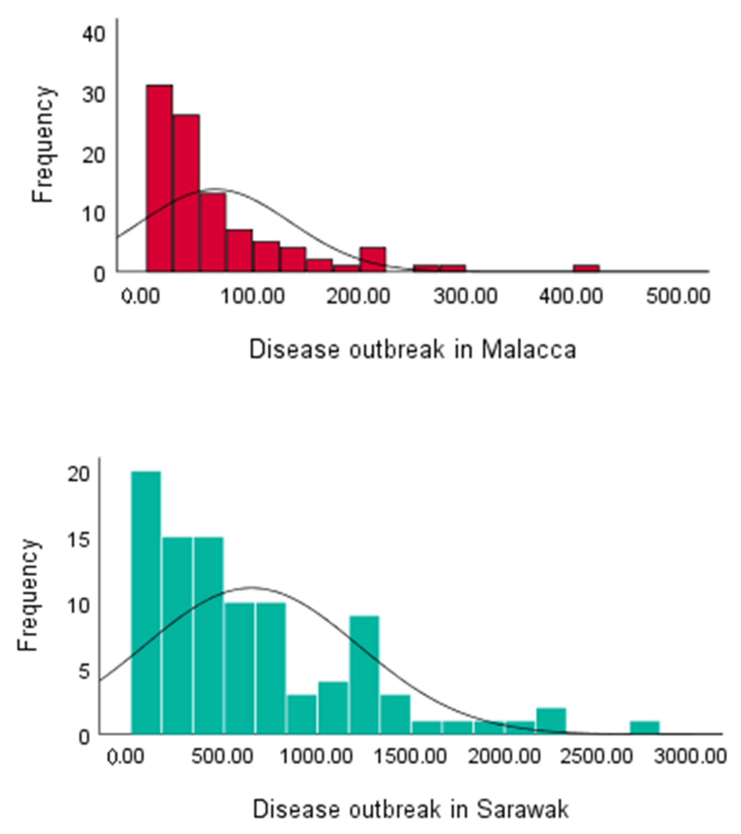
| Disease outbreak | 6220 | Malacca | 64.719 | 69.924 | 1.078 |
| 62061 | Sarawak | 646.468 | 573.597 | 0.887 | |
| Humidity (%) | 6220 | Malacca | 75.704 | 1.185 | 0.015 |
| 62061 | Sarawak | 75.150 | 0.821 | 0.010 |
| Feature | Ratio | Lower Bound | Upper Bound | |
|---|---|---|---|---|
| Proposed Method | Disease outbreak | 1.216 | 1.122 | 1.309 |
| Humidity (%) | 1.431 | 0.571 | 2.292 | |
| Yue and Baleanu’s method | Disease outbreak | 1.216 | 1.078 | 1.353 |
| Humidity (%) | 1.431 | 0.253 | 2.610 | |
Publisher’s Note: MDPI stays neutral with regard to jurisdictional claims in published maps and institutional affiliations. |
© 2022 by the authors. Licensee MDPI, Basel, Switzerland. This article is an open access article distributed under the terms and conditions of the Creative Commons Attribution (CC BY) license (https://creativecommons.org/licenses/by/4.0/).
Share and Cite
Bahrampour, A.; Avazzadeh, Z.; Mahmoudi, M.R.; Lopes, A.M. Improved Confidence Interval and Hypothesis Testing for the Ratio of the Coefficients of Variation of Two Uncorrelated Populations. Mathematics 2022, 10, 3495. https://doi.org/10.3390/math10193495
Bahrampour A, Avazzadeh Z, Mahmoudi MR, Lopes AM. Improved Confidence Interval and Hypothesis Testing for the Ratio of the Coefficients of Variation of Two Uncorrelated Populations. Mathematics. 2022; 10(19):3495. https://doi.org/10.3390/math10193495
Chicago/Turabian StyleBahrampour, Abbas, Zeynab Avazzadeh, Mohammad Reza Mahmoudi, and António M. Lopes. 2022. "Improved Confidence Interval and Hypothesis Testing for the Ratio of the Coefficients of Variation of Two Uncorrelated Populations" Mathematics 10, no. 19: 3495. https://doi.org/10.3390/math10193495
APA StyleBahrampour, A., Avazzadeh, Z., Mahmoudi, M. R., & Lopes, A. M. (2022). Improved Confidence Interval and Hypothesis Testing for the Ratio of the Coefficients of Variation of Two Uncorrelated Populations. Mathematics, 10(19), 3495. https://doi.org/10.3390/math10193495