Pricing European and American Installment Options

Abstract

This paper derives accurate and efficient analytic approximations for the prices of both European and American continuous-installment call and put options. The solutions are in the form of series in time-to-expiry with explicit formulae for the coefficients provided. Unlike other solutions for installment options, no Laplace inverses are needed, and there is no need to solve complex, recursive systems or integral equations. The formulae provided fast yield and accurate solutions not just for the prices, but also for the critical boundaries. We also compare the solutions with those obtained using an existing method and show that it surpasses it delivering more correct option prices and critical stock prices.

1. Introduction

Installment options are contracts in which investors pay the purchase price, or premium, in installments over the life of the option and give the investors the flexibility to abandon the option early if they so desire. The investor of an installment option pays a minimum premium at the opening of the contract and can then decide whether to maintain the option by continuing with the installment payments, or else abandon the option by discontinuing installment payments. Because of the opportunity to be able to abandon the installment option early, the sum total of the premium for the installment option is always higher than for the premium of the corresponding vanilla option. However, with the reduction in the up-front premium, compared to other financial derivatives, installment options are traded actively on exchanges as well as on over-the-counter (OTC) markets. In particular, installment options are popular in Foreign Exchange markets, where there is uncertainty in the future cash flow. (An investor who needs to buy a particular currency in the future and fears the exchange rate will increase can lock in an exchange rate by buying the currency installment call option. With the installment option, the investor can split the premium over time. In the instance that a corresponding vanilla call option is out-of-the-money, then even selling the vanilla before expiry would probably not give him as much as the amount between the vanilla and the sum of the installment payments to date.) Applications of installment options have also been identified in real options models. For instance, rent-to-own and contract-for-deed sales in residential real estate can be analyzed as installment call options (see e.g., [1]). Another example is the funding by Venture Capital (VC) which provides companies with initial funding for projects and then further funding at later times, provided the companies meet prescribed targets. If the company fails to meet the target at some stage, the VC investor can abandon the project with no recovery value (see [2]). Further, installment options are often used by pension fund managers to safeguard their portfolios at a lower fee, as well as being used in other markets such as equity and interest rate markets.

The installment payments themselves may be paid discretely (DI) on a finite number of exercise dates, or else continuously (CI) in a succession of installments, at a given rate per unit time. As well as European-style installment options, there are also American-style installment options, whereby the holder may not only choose to exit the option early, but can also choose to exercise the option early.

For European DI options, Davis et al. ([3,4]) obtained no-arbitrage bounds on the initial premium by using the ideas of compound options and NPV. This was carried out in the Black–Scholes–Merton framework [5]. Then, Griebsch et al. [6] derived a closed-form formula for the value of the DI option, which was expressed in terms of multidimensional cumulative normal distribution functions.

Solving the CI options price, however, is more complicated, and no known exact solution has been found to date. For European CI options, Alobaidi, et al. [7] used a partial Laplace transform of the governing nonhomogeneous partial differential equation (PDE) for the value of the option and investigated the asymptotic properties of the optimal stopping boundary near expiry. Kimura [8] obtained an explicit Laplace transform of the initial premium of the European CI, as well as its Greeks. However, inverting Laplace transforms is difficult and needs to be performed numerically. To show how this can be achieved, Mezentsev et al. [9] investigated the Kryzhnyi method for the numerical inverse Laplace transformation and applied it to the European CI option pricing problem. They compared their results with other classical methods for the inversion of Laplace transforms.

In a different approach, Yi et al. [10] considered a parabolic variational inequality that arises from valuing the European installment put option and established the existence and uniqueness of the solution to the problem. In 2011, Ciurlia [11] derived integral expressions for the initial premium as well as the optimal stopping boundary. He also posed the problem as an optimal stopping problem and then used a Monte Carlo (MC) approach to solve it. Then, Jeon and Kim [12], examined the pricing of European CI currency options in the mean-reversion environment. They derived the integral equation representation for the optimal stopping boundary using Mellin transforms and compared their results with the least square MC method.

American CI options can be exercised early, and so the solution to these involves not one, but two free boundaries. This adds to the complexity of the problem. Ciurlia and Roko [13] formulated the solution of the initial premium for the American CI option in terms of integrals. Then, they applied the multi-piece exponential function (MEF) method to the valuation formulas. They compared their results with those found from the finite-difference and Monte Carlo methods. Their method, however, has a major shortcoming, as the MEF method produces a discontinuity in the optimal stopping and early exercise boundaries. More recently, in [14], Kimura explicitly found the Laplace transform of the initial premium. This was expressed in terms of the value of the corresponding European option (with the same payoff) and the premiums from early exercise and halfway cancelation. He also obtained a pair of nonlinear equations for the Laplace transforms of the boundaries. Ciurlia and Caperdoni [15] extended the analysis to the perpetual CI case.

Furthering their work on European CI options, Yang and Yi [16] considered a parabolic variational inequality problem resulting from the American-style CI options. They also proved the existence and uniqueness of the solution to the American CI option valuation. Ciurlia [17] extended his work on European CI options and presented an integral equation approach for the valuation of American-style CI options. Using a Fourier transform-based solution technique, he formulated a system of coupled recursive integral equations for the value of the two free boundaries. He then formulated an analytic representation of the option price.

Other authors have considered different types of CI options and/or other types of underlying processes for the Geometric Brownian motion. In [18] Huang et al. considered the pricing of the American CI option on a bond under an interest rate model. Deng [19] considered the pricing of a barrier-type American CI option. Deng and Xue [20] price American-style CI options under the constant elasticity of variance (CEV) diffusion model for the asset price. Deng [21] uses an integral equation approach to price American CI options when the stock price is assumed to follow Heston’s stochastic volatility model.

The solution method employed in this paper is based on a modification of the method used by Medvedev and Scaillet [22] to price American put options. In their paper, the authors present a new analytical approximation method that they say ‘is both computationally tractable and general enough to be successfully applied to a three factor diffusion model without jumps’. Their approach is to replace the used optimal exercise rule with a simple suboptimal exercise rule to exercise the option when its level of moneyness (measured in standard deviations) reaches a particular level. The price for the American option is written as an infinite series with respect to time-to-expiry. However, finding the coefficients of their series solution involves solving complicated recursive systems.

In this paper, we derive analytical approximations for both European and American CI call and put options, in the form of series solutions for which explicit formulae for the coefficients are given. The European CI call (put) option has one critical boundary below (above), for which the option should be withdrawn, and the American call (put) has two critical boundaries; one boundary, below (above), for which the option should be withdrawn and the other boundary above (below) for which the option should be exercised. We derive analytical approximations for all these boundaries. To find the solution, as stated above, we adapt the method of Medvedev and Scaillet in a different form, such that we are able to solve for coefficients in the series solution without having to solve complicated recursive systems. This then leads to fast results. We then compare the performance of our models with the numerical finite-difference Crank–Nicolson method, which is used as the proxy to the true solution. The method presented in this paper is found to yield very accurate and efficient option prices. Quite often, methods that lead to accurate option prices do not achieve very accurate critical stock prices. However, our method was found to achieve excellent accuracy for critical stock prices as well as the option prices. Further, we compare our European CI prices with those obtained via Kimura’s analytic approximation method [8] and find that our method outperformed Kimura’s method for both option values and exit boundaries. We also examine the behavior of the free boundaries near expiry and find that the exit/withdrawal boundary acts similarly with respect to expiry time in all cases, independent of the level of the other parameters. However, the behavior of the early exercise boundaries for the American CI options depends on a relationship between the interest rate, dividend yield, strike price, and installment rate.

2. The Mathematical Model and Solutions for the American and European CI Options

In this section, we present the main result of the paper for the CI call options, whereby we give the series representations for the American and European CI call prices as well as the associated critical boundaries. These series depend on coefficients for which explicit formulae are given. As the solution procedure for the CI put options is very similar, we have provided the solutions to the European and American CI put options in Appendix A and Appendix B, respectively.

Suppose that the price of American and European CI options (either calls or puts), with exercise price X and expiry T are given by $V_a(S,t)$ and $V_e(S,t)$, respectively, where the stock price S follows the usual risk-neutral log normal process, i.e.,

$$dS/S=(r-q)dt+\sigma dZ,$$

(1)

where $r,q,\sigma >0,$ are, respectively, the constant risk-free interest rate, dividend yield, and volatility and Z is a Wiener process under a risk-neutral measure. Additionally, suppose that the continuous installment rate is $L>0,$ so that in a time $dt$, the holder pays the amount $Ldt$ in order to continue the contract.

Then, in the continuation region of the contracts, both $V_a(S,t)$ and $V_e(S,t)$ satisfy the partial differential equation (PDE) (see e.g., [23])

$$V_t+\frac{{\sigma }^2{S}^2}{2}{V}_{SS}+(r-q)S{V}_S-rV=L.$$

(2)

We note that without the term L, (2) is the usual Black–Scholes PDE [5].

2.1. American CI Call Option Valuation

If we denote the upper critical optimal exercise boundary (OEB), above which the option should be exercised, by $S_e(T-t)$ and the lower critical boundary below which the option should expire or withdrawn (and so is worthless) by $S_w(T-t)$, then the continuation region for the American CI call option is $S_w(T-t)\le S\le S_e(T-t)$ and $V=V_a(S,t)$ needs to satisfy (2) subject to

$$\begin{array}{ccc}\hfill V(S,T)& =& max(S-X,0),\hfill \end{array}$$

(3a)

$$\begin{array}{ccc}\hfill V(S_e(T-t),t)& =& S_e(T-t)-X,\hfill \end{array}$$

(3b)

$$\begin{array}{ccc}\hfill V_S(S_e(T-t),t)& =& 1,\hfill \end{array}$$

(3c)

$$\begin{array}{ccc}\hfill V(S_w(T-t),t)& =& 0,\hfill \end{array}$$

(3d)

$$\begin{array}{ccc}\hfill V_S(S_w(T-t),t)& =& 0.\hfill \end{array}$$

(3e)

As mentioned in the Introduction, our solution method is based on an approach due to Medvedev and Scaillet [22]. In pricing an American put option with price $P(S,t)$ with free boundary $S_f(T-t)$, Medvedev and Scaillet [22] substituted the smooth-pasting condition $P_S(S_f(T-t),t)=-1$ with an explicit exercise rule and presumed that the critical boundary, the optimal exercise boundary (OEB), was of the specific form

$$S_f(T-t)=X{e}^{-y\sigma \sqrt{T-t}},$$

(4)

where y is a decision variable which determines the suboptimal rule. In our current problem, for the American CI, we have two free boundaries. However, we will use a similar idea for both of the free boundaries of the American CI option and, unlike Medvedev and Scaillet, give explicit formulae for the coefficients in the series representation for the American CI. The following theorem gives our main solution for the American CI call option.

Theorem 1.

Define $x=ln(X/S)$ and $\tau =T-t.$ An approximation of the short-term American CI call option price in $S_w\left(\tau \right)\le S\le S_e\left(\tau \right),$ where $S_e\left(\tau \right)$ and $S_w\left(\tau \right)$, respectively, are the exercise (upper) and withdraw (lower) critical boundaries, is

$$V(x,\tau )=\underset{z\ge \frac{x}{\sigma \sqrt{\tau }},y\ge -\frac{x}{\sigma \sqrt{\tau }}}{max}V(x,\tau ;y,z)=V(x,\tau ;\widehat{y},\widehat{z}),$$

(5)

where

$$\begin{array}{ccc}\hfill V(x,\tau ;y,z)& =& -\frac{L}{r}+e^{-q\tau }{e}^{Ax+B\tau }\left\{\frac{L}{r}+e^{\frac{-x^2}{2{\sigma }^2\tau }}\sum _{i=1}^{\infty }{\tau }^{i/2}\left[C_{i}M\left(\frac{1+i}{2},\frac{1}{2},\frac{x^2}{2{\sigma }^2\tau }\right)\right.\right.\hfill \\ & & \left.\left.+D_{i}U\left(\frac{1+i}{2},\frac{1}{2},\frac{x^2}{2{\sigma }^2\tau }\right)\right]\right\}\hfill \\ & & forln\left(\frac{X}{S_e\left(\tau \right)}\right)\le x\le 0(i.e.,X\le S\le S_e\left(\tau \right)),\hfill \end{array}$$

(6)

$$\begin{array}{ccc}& =& -\frac{L}{r}+e^{-q\tau }{e}^{Ax+B\tau }\left\{\frac{L}{r}+e^{\frac{-x^2}{2{\sigma }^2\tau }}\sum _{i=1}^{\infty }{\tau }^{i/2}\left[\left(C_i+\frac{2D_i\sqrt{\pi }}{\mathrm{\Gamma }(1+i/2)}\right)M\left(\frac{1+i}{2},\frac{1}{2},\frac{x^2}{2{\sigma }^2\tau }\right)\right.\right.\hfill \\ & & \left.\left.-D_{i}U\left(\frac{1+i}{2},\frac{1}{2},\frac{x^2}{2{\sigma }^2\tau }\right)\right]\right\}\hfill \\ & & for 0<x\le ln\left(\frac{X}{S_w\left(\tau \right)}\right)(i.e.,S_w\left(\tau \right)\le S<X),\hfill \end{array}$$

(7)

with $A=\frac{r-q-\frac{{\sigma }^2}{2}}{{\sigma }^2},B=-\frac{{(r-q+\frac{{\sigma }^2}{2})}^2}{2{\sigma }^2}$ and M and U representing the Kummer-M and Kummer-U functions, respectively (see [24]).

The coefficients $C_i$ and $D_i$ are given by

$$\begin{array}{ccc}\hfill C_i& =& \frac{{\left({\rho }_1\right)}_i{U}^y-{\left({\rho }_2\right)}_i{\left({\rho }_3\right)}_i}{M^z{U}^y-M^y{\left({\rho }_2\right)}_i}\hfill \end{array}$$

(8)

$$\begin{array}{ccc}\hfill D_i& =& \frac{M^z{\left({\rho }_3\right)}_i-{\left({\rho }_1\right)}_i{M}^y}{M^z{U}^y-M^y{\left({\rho }_2\right)}_i}\hfill \end{array}$$

(9)

where

$$\begin{array}{ccc}\hfill {\left({\rho }_1\right)}_i& =& \frac{L}{r}{\psi }_i{e}^{\frac{z^2}{2}}\hfill \end{array}$$

(10a)

$$\begin{array}{ccc}\hfill {\left({\rho }_2\right)}_i& =& \frac{2\sqrt{\pi }}{\mathrm{\Gamma }(1+\frac{i}{2})}{M}_z-U_z\hfill \end{array}$$

(10b)

$$\begin{array}{ccc}\hfill {\left({\rho }_3\right)}_i& =& \left(X{\gamma }_i+(\frac{L}{r}-X){\widehat{ϵ}}_i\right)e^{y^2/2}\hfill \end{array}$$

(10c)

$$\begin{array}{ccc}\hfill M^y& =& M\left(\frac{1+i}{2},\frac{1}{2},\frac{y^2}{2}\right),M^z=M\left(\frac{1+i}{2},\frac{1}{2},\frac{z^2}{2}\right),\hfill \end{array}$$

(10d)

$$\begin{array}{ccc}\hfill U^y& =& U\left(\frac{1+i}{2},\frac{1}{2},\frac{y^2}{2}\right),U^z=U\left(\frac{1+i}{2},\frac{1}{2},\frac{z^2}{2}\right),\hfill \end{array}$$

(10e)

$$\begin{array}{ccc}\hfill {\widehat{ϵ}}_i& =& \sum _{j=0}^i{ϵ}_j{b}_{i-j},{\gamma }_i=\sum _{j=0}^i{b}_j{\left({\beta }^{\prime }\right)}_{i-j},{\psi }_i=\sum _{j=0}^i{a}_j{b}_{i-j},\hfill \end{array}$$

(10f)

with

$$b_n=\left\{\begin{array}{cc}0\hfill & n=1,3,5,...\hfill \\ \frac{{(q-B)}^{n/2}}{(n/2)!}\hfill & n=0,2,4,...\hfill \end{array}\right.$$

(10g)

$$a_m=\frac{{(-Az\sigma )}^m}{m!},m=0,1,2,3...$$

(10h)

$${ϵ}_m=\frac{{\left(Ay\sigma \right)}^m}{m!},m=0,1,2,3...$$

(10i)

$${\beta }_m^{\prime }=\frac{{\left((1+A)y\sigma \right)}^m}{m!},m=0,1,2,3,...$$

(10j)

The upper (exercise) and lower (withdraw) critical boundaries are given, respectively, by

$$S_e\left(\tau \right)=X{e}^{y\sigma \sqrt{\tau }}$$

(11)

and

$$S_w\left(\tau \right)=X{e}^{-z\sigma \sqrt{\tau }},$$

(12)

$y,z\ge 0$, where approximations ${\widehat{\theta }}_1,$${\widehat{\theta }}_2$ for the true early exercise level of moneyness, are given by

$${\widehat{\theta }}_1\left(\tau \right)=\underset{\theta =\frac{x}{\sigma \sqrt{\tau }}}{min}\{\theta \le 0:\widehat{y}(\theta ,\tau )=-\theta \},$$

(13)

and

$${\widehat{\theta }}_2\left(\tau \right)=\underset{\theta =\frac{x}{\sigma \sqrt{\tau }}}{min}\{\theta \ge 0:\widehat{z}(\theta ,\tau )=\theta \},$$

(14)

where $\widehat{y}$ and $\widehat{z}$ are implicitly defined in (5) or as ${argmax}_{z\ge \frac{x}{\sigma \sqrt{\tau }},y\ge -\frac{x}{\sigma \sqrt{\tau }}}V(x,\tau ;y,z)$.

Proof. 

We begin by turning (2) into a homogeneous, forward equation by letting $V=W-L/r$ and $\tau =T-t$ to get

$$W_{\tau }=\frac{{\sigma }^2{S}^2}{2}{W}_{SS}+(r-q)S{W}_S-rW,$$

(15)

to be solved subject to

$$\begin{array}{ccc}\hfill W(S,0)& =& max(S-X,0)+L/r,\hfill \end{array}$$

(16a)

$$\begin{array}{ccc}\hfill W(S_e\left(\tau \right),\tau )& =& S_e\left(\tau \right)-X+L/r,\hfill \end{array}$$

(16b)

$$\begin{array}{ccc}\hfill W_S(S_e\left(\tau \right),\tau )& =& 1,\hfill \end{array}$$

(16c)

$$\begin{array}{ccc}\hfill W(S_w\left(\tau \right),\tau )& =& L/r,\hfill \end{array}$$

(16d)

$$\begin{array}{ccc}\hfill W_S(S_w\left(\tau \right),\tau )& =& 0.\hfill \end{array}$$

(16e)

It is useful to separate the continuation domain into the two regions $S_w\left(\tau \right)\le S<X$ and $X\le S\le S_e\left(\tau \right)$. In the continuation region of the American CI call option, $W(S,\tau )$ satisfies Equation (15), which in

$S_w\left(\tau \right)\le S<X$ needs to be solved subject to

$$W(S_w\left(\tau \right),\tau )=L/r,$$

(17)

and in $X\le S<S_e\left(\tau \right)$, subject to $W(S_e\left(\tau \right),\tau )=S_e\left(\tau \right)-X+L/r.$

Note: We will introduce the transformation $\theta =\frac{x}{\sigma \sqrt{\tau }},x=ln\left(\frac{X}{S}\right)$ and through this transformation, the condition at $\tau =0$ is shifted to infinity. As the continuation region will be a finite interval, $-y\le \theta \le z$, we actually avoid the condition at expiry.

We also require continuity of the option’s value and its derivative over the strike price X, i.e.,

$$\begin{array}{ccc}\hfill \underset{S\to X^{-}}{lim}W& =& \underset{S\to X^{+}}{lim}W,\hfill \end{array}$$

$$\begin{array}{ccc}\hfill \underset{S\to X^{-}}{lim}{W}_S& =& \underset{S\to X^{+}}{lim}{W}_S.\hfill \end{array}$$

For an exact, classical solution to PDE (2), we would also require continuity of $V_{SS}$ (the second derivative) across the strike price. However, this will follow automatically, as will be seen in the proof.

Making the substitutions

$$S=X{e}^{-x},W=e^{-q\tau }Y(x,\tau ),$$

PDE (15) becomes

$$Y_{\tau }=\frac{{\sigma }^2}{2}{Y}_{xx}+\left[\frac{{\sigma }^2}{2}+(q-r)\right]Y_x-(r-q)Y.$$

(18)

We solve (18) on $(-y\sigma \sqrt{\tau },0)$ subject to $Y(-y\sigma \sqrt{\tau },\tau )=e^{q\tau }[X{e}^{y\sigma \sqrt{\tau }}-X+L/r]$ and on $(0,z\sigma \sqrt{\tau })$ subject to $Y(z\sigma \sqrt{\tau },\tau )=e^{q\tau }L/r.$ The continuity conditions become

$$\begin{array}{ccc}\hfill \underset{x\to 0^{-}}{lim}Y& =& \underset{x\to 0^{+}}{lim}Y,\hfill \\ \hfill \underset{x\to 0^{-}}{lim}{Y}_x& =& \underset{x\to 0^{+}}{lim}{Y}_x.\hfill \end{array}$$

We let $Y=exp(Ax+B\tau )u(x,\tau )$ where $A=\frac{r-q-\frac{{\sigma }^2}{2}}{{\sigma }^2},B=\frac{{\sigma }^2{A}^2}{2}+A(q-r+\frac{{\sigma }^2}{2})-(r-q)$ which reduces (18) to the classical heat equation

$$u_{\tau }=\frac{{\sigma }^2}{2}{u}_{xx}.$$

(19)

Lastly, we let $\theta =\frac{x}{\sigma \sqrt{\tau }}$ to get

$$2\tau u_{\tau }=u_{\theta \theta }+\theta u_{\theta },$$

(20)

to be solved on $-y\le \theta \le 0$ subject to

$$u(-y,\tau )=exp(Ay\sigma \sqrt{\tau }-B\tau )exp\left(q\tau \right)[Xexp\left(y\sigma \sqrt{\tau }\right)-X+L/r],$$

(21)

and on $0<\theta \le z$ subject to

$$u(z,\tau )=exp(-Az\sigma \sqrt{\tau }-B\tau )exp\left(q\tau \right)L/r.$$

(22)

The continuity conditions are

$$\begin{array}{ccc}\hfill \underset{\theta \to 0^{-}}{lim}u& =& \underset{\theta \to 0^{+}}{lim}u,\hfill \end{array}$$

$$\begin{array}{ccc}\hfill \underset{\theta \to 0^{-}}{lim}{u}_{\theta }& =& \underset{\theta \to 0^{+}}{lim}{u}_{\theta }.\hfill \end{array}$$

Equation (20) has separable solutions of the type

$$u(\theta ,\tau )=e^{\frac{-{\theta }^2}{2}}\sum _{i=1}^{\infty }{\tau }^{\frac{i}{2}}\left[C_{i}M\left(\frac{1+i}{2},\frac{1}{2},\frac{{\theta }^2}{2}\right)+D_{i}U\left(\frac{1+i}{2},\frac{1}{2},\frac{{\theta }^2}{2}\right)\right],$$

(23)

where M and U are, respectively, the Kummer-M and Kummer-U functions. In (23), the separation constant that was used is ${\lambda }_i=\frac{i}{2}$, where i is a positive integer. This is because it has been shown (see e.g., [25]) that series in the square root of time have been successful in solving other linear diffusion equations which involve free boundaries. We will use (23) to describe the solutions in $-y\le \theta \le 0$.

For $0<\theta \le z$, we use different constants and write

$$u(\theta ,\tau )=e^{\frac{-{\theta }^2}{2}}\sum _{i=1}^{\infty }{\tau }^{\frac{i}{2}}\left[F_{i}M\left(\frac{1+i}{2},\frac{1}{2},\frac{{\theta }^2}{2}\right)+G_{i}U\left(\frac{1+i}{2},\frac{1}{2},\frac{{\theta }^2}{2}\right)\right].$$

(24)

Determining the Solution Coefficients

In order to satisfy the limit conditions at $\theta =0$, we need

$$\begin{array}{ccc}\hfill C_i+D_i\frac{\sqrt{\pi }}{\mathrm{\Gamma }(1+\frac{i}{2})}& =& F_i+G_i\frac{\sqrt{\pi }}{\mathrm{\Gamma }(1+\frac{i}{2})},\hfill \end{array}$$

(25)

$$\begin{array}{ccc}\hfill D_i& =& -G_i.\hfill \end{array}$$

(26)

Hence, we set ${\displaystyle F_i=C_i+\frac{2\sqrt{\pi }}{\mathrm{\Gamma }(1+\frac{i}{2})}{D}_i}$ and $G_i=-D_i$.

We now note that for continuity at $x=0$ of the second derivative, we need

$$i{C}_i+i{D}_i\frac{\sqrt{\pi }}{\mathrm{\Gamma }(1+\frac{i}{2})}=i{F}_i+i{G}_i\frac{\sqrt{\pi }}{\mathrm{\Gamma }(1+\frac{i}{2})}.$$

This, however, follows automatically from (25). This means that at $x=0$, derivatives of all orders are continuous.

Hence, we have

$$\begin{array}{ccc}\hfill u(\theta ,\tau )& =& e^{\frac{-{\theta }^2}{2}}\sum _{i=1}^{\infty }{\tau }^{i/2}\left[C_{i}M\left(\frac{1+i}{2},\frac{1}{2},\frac{{\theta }^2}{2}\right)+D_{i}U\left(\frac{1+i}{2},\frac{1}{2},\frac{{\theta }^2}{2}\right)\right]\hfill \\ & & \mathrm{for} -y\le \theta \le 0,\hfill \\ & =& e^{\frac{-{\theta }^2}{2}}\sum _{i=1}^{\infty }{\tau }^{i/2}\left[\left(C_i+\frac{2D_i\sqrt{\pi }}{\mathrm{\Gamma }(1+i/2)}\right)M\left(\frac{1+i}{2},\frac{1}{2},\frac{{\theta }^2}{2}\right)\right.\hfill \\ & & -D_i\left.U\left(\frac{1+i}{2},\frac{1}{2},\frac{{\theta }^2}{2}\right)\right]\hfill \\ & & \mathrm{for} 0<\theta \le z,\hfill \end{array}$$

(27)

To find the constants $C_i$ and $D_i$, we initially apply the boundary condition at $\theta =-y$. In series form, the condition there is

$$u(-y,\tau )=\sum _{i=0}^{\infty }[X{\gamma }_i+(L/r-X){\widehat{ϵ}}_i]{\tau }^{i/2},$$

(28)

where ${\widehat{ϵ}}_i$ and ${\gamma }_i$ are defined in (10f)–(10j). Hence, equating coefficients of ${\tau }^{i/2}$, we get

$${\displaystyle D_i=\frac{[X{\gamma }_i+(L/r-X){\widehat{ϵ}}_i]e^{y^2/2}-C_{i}M\left(\frac{1+i}{2},\frac{1}{2},\frac{y^2}{2}\right)}{U\left(\frac{1+i}{2},\frac{1}{2},\frac{y^2}{2}\right)},}$$

(29)

We now apply the boundary condition at $\theta =z.$ The condition there in series form is

$$u(z,\tau )=\frac{L}{r}\sum _{i=0}^{\infty }{\psi }_i{\tau }^{i/2},$$

(30)

where ${\psi }_i$ is defined in (10f)–(10j). Hence, equating coefficients of ${\tau }^{i/2}$, we get

$$\frac{L}{r}{\psi }_i=e^{-z^2/2}\left[\left(C_i+\frac{2D_i\sqrt{\pi }}{\mathrm{\Gamma }(1+i/2)}\right)M\left(\frac{1+i}{2},\frac{1}{2},\frac{z^2}{2}\right)-D_{i}U\left(\frac{1+i}{2},\frac{1}{2},\frac{z^2}{2}\right)\right].$$

(31)

Solving (29) and (31), we get $C_i$ and $D_i$ as given in (8) and (9).

The conditions for early exercise and exit (13) and (14), respectively, are derived by realizing that with $\theta =\frac{x}{\sigma \sqrt{\tau }}$, if $\theta =-\widehat{y}(\theta ,\tau )$ or $\theta =\widehat{z}(\theta ,\tau )$ then the option should be exercised/withdrawn. □

2.2. European CI Call Option Valuation

We now concentrate on the European CI call option, where the early exercise feature is not available. We will denote the critical boundary, below which the option should expire (and so has zero value) by $S_z(T-t)$, and so the continuation region for the European CI option is $S_z(T-t)\le S<\infty$ and $V=V_e(S,t)$ needs to satisfy (2) subject to

$$\begin{array}{ccc}\hfill V(S,T)& =& max(S-X,0),\hfill \end{array}$$

(32a)

$$\begin{array}{ccc}\hfill V(S_z(T-t),t)& =& 0,\hfill \end{array}$$

(32b)

$$\begin{array}{ccc}\hfill V_S(S_z(T-t),t)& =& 0.\hfill \end{array}$$

(32c)

We now give the analytic approximation for the European CI call option in the following theorem. As the proof follows the same lines as Theorem 1, it will be omitted.

Theorem 2.

Let $x=ln(X/S)$ and $\tau =T-t.$ An approximation to the short-term European CI call option price in $S_z\left(\tau \right)\le S\le \infty ,$ where $S_z\left(\tau \right)$ is the exit (or withdrawal) and OEB is

$$V(x,\tau )=\underset{z\ge \frac{x}{\sigma \sqrt{\tau }}}{max}V(x,\tau ;z)=V(x,\tau ;\widehat{z}),$$

(33)

where

$$\begin{array}{ccc}\hfill V(x,\tau ;z)& =& -\frac{L}{r}+e^{-q\tau }{e}^{Ax+B\tau }\left\{\frac{L}{r}+e^{\frac{-x^2}{2{\sigma }^2\tau }}\sum _{i=1}^{\infty }{\tau }^{i/2}\left[C_{i}M\left(\frac{1+i}{2},\frac{1}{2},\frac{x^2}{2{\sigma }^2\tau }\right)\right.\right.\hfill \\ & & \left.\left.+D_{i}U\left(\frac{1+i}{2},\frac{1}{2},\frac{x^2}{2{\sigma }^2\tau }\right)\right]\right\}\hfill \\ & & for-\infty \le x\le 0(i.e.,X\le S\le \infty ),\hfill \end{array}$$

(34)

$$\begin{array}{ccc}& =& -\frac{L}{r}+e^{-q\tau }{e}^{Ax+B\tau }\left\{\frac{L}{r}+e^{\frac{-x^2}{2{\sigma }^2\tau }}\sum _{i=1}^{\infty }{\tau }^{i/2}\left[\left(C_i+\frac{2D_i\sqrt{\pi }}{\mathrm{\Gamma }(1+i/2)}\right)M\left(\frac{1+i}{2},\frac{1}{2},\frac{x^2}{2{\sigma }^2\tau }\right)\right.\right.\hfill \\ & & \left.\left.-D_{i}U\left(\frac{1+i}{2},\frac{1}{2},\frac{x^2}{2{\sigma }^2\tau }\right)\right]\right\}\hfill \\ & & for 0<x\le ln\left(\frac{X}{S_z\left(\tau \right)}\right)(i.e.,S_z\left(\tau \right)\le S<X),\hfill \end{array}$$

(35)

with $A=\frac{r-q-\frac{{\sigma }^2}{2}}{{\sigma }^2},B=-\frac{{(r-q+\frac{{\sigma }^2}{2})}^2}{2{\sigma }^2}$, and M and U represent the Kummer-M and Kummer-U functions, respectively, (see [24]).

The coefficients $C_i$ and $D_i$ are given by

$$\begin{array}{ccc}\hfill C_i& =& \frac{\mathrm{\Gamma }\left(\frac{(1+i)}{2}\right){\left(2{\sigma }^2\right)}^{i/2}}{\sqrt{\pi }}\left[\frac{X{(A+1)}^i}{i!}+\left(\frac{L}{r}-X\right)\frac{A^i}{i!}\right]\hfill \end{array}$$

(36)

$$\begin{array}{ccc}\hfill D_i& =& \frac{\left[\frac{L}{r}{\psi }_i{e}^{\frac{z^2}{2}}-C_{i}M\left(\frac{1+i}{2},\frac{1}{2},\frac{z^2}{2}\right)\right]}{\frac{2\sqrt{\pi }}{\mathrm{\Gamma }(1+\frac{i}{2})}M\left(\frac{1+i}{2},\frac{1}{2},\frac{z^2}{2}\right)-U\left(\frac{1+i}{2},\frac{1}{2},\frac{z^2}{2}\right)}\hfill \end{array}$$

(37)

where

$$\begin{array}{c}\hfill {\psi }_i=\sum _{j=0}^i{a}_j{b}_{i-j},\end{array}$$

(38a)

with

$$b_n=\left\{\begin{array}{cc}0\hfill & n=1,3,5,...\hfill \\ \frac{{(q-B)}^{n/2}}{(n/2)!}\hfill & n=0,2,4,...\hfill \end{array}\right.$$

(38b)

$$a_m=\frac{{(-Az\sigma )}^m}{m!},m=0,1,2,3...$$

(38c)

The withdraw/exit critical boundary is given by

$$S_z\left(\tau \right)=X{e}^{-z\sigma \sqrt{\tau }},$$

(39)

$z\ge 0$, where the approximation ${\widehat{\theta }}_0$ for the true early exercise level of moneyness is

$${\widehat{\theta }}_0\left(\tau \right)=\underset{\theta =\frac{x}{\sigma \sqrt{\tau }}}{min}\{\theta \ge 0:\widehat{z}(\theta ,\tau )=\theta \},$$

(40)

where $\widehat{z}$ is implicitly defined in (33) or explicitly as ${argmax}_{z\ge \frac{x}{\sigma \sqrt{\tau }}}V(x,\tau ;z).$

3. Early Exercise Price at Short Times to Expiry

At $\tau =0$, we know (see, e.g., Kimura [14]) that for American CI call options $S_e=max\left(\frac{rX-L}{q},X\right)$ and $S_w\left(0\right)=X$, while for European CI call options we have $S_z\left(0\right)=X$. We now examine the behavior of the free boundaries near $\tau =0$, remembering that we defined $\theta =\frac{x}{\sigma \sqrt{\tau }}$ where $x=ln\left(\frac{X}{S}\right)$.

3.1. American Case

We now demonstrate how our representation of the solution gives an approximation ${\widehat{\theta }}_2$ of the early withdrawal level for the lower boundary $S_w$ in (12) as $\tau$ tends to zero, which is independent of $r,q,$ and $L>0$.

Proposition 1.

Solution (5) leads to an approximation ${\widehat{\theta }}_2$ of the early withdrawal/exit level in (12) that is $\sim \sqrt{ln(1/\tau )}$ as τ tends to zero.

Proof. 

We have in $0\le \theta \le z$,

$$\begin{array}{ccc}\hfill V(\theta ,\tau ;y,z)& =& e^{-q\tau }{e}^{A\sigma \sqrt{\tau }\theta }{e}^{B\tau }\left\{\frac{L}{r}+e^{-{\theta }^2/2}\left[\sqrt{\tau }\left\{(C_1+4D_1)M\left(1,\frac{1}{2},\frac{{\theta }^2}{2}\right)-D_{1}U\left(1,\frac{1}{2},\frac{{\theta }^2}{2}\right)\right\}\right.\right.\hfill \\ & +& \left.\left.R(\theta ,\tau ;y,z)\tau \right]\right\}-\frac{L}{r},\hfill \end{array}$$

where

$${\displaystyle R(\theta ,\tau ;y,z)=\sum _{i=2}^{\infty }{\tau }^{\frac{i-2}{2}}\left[\left(C_i+\frac{2D_i\sqrt{\pi }}{\mathrm{\Gamma }(1+i/2)}\right)M\left(\frac{1+i}{2},\frac{1}{2},\frac{{\theta }^2}{2}\right)-D_{i}U\left(\frac{1+i}{2},\frac{1}{2},\frac{{\theta }^2}{2}\right)\right].}$$

From (14), we have for small $\tau$ that $V_z({\tilde{\theta }}_2,\tau ;\infty ,{\tilde{\theta }}_2)=0$. From this we get

$$\begin{array}{c}\hfill \sqrt{\tau }\left\{{(C_1+4D_1)}_{z}M\left(1,\frac{1}{2},\frac{{\widehat{\theta }}_2^2}{2}\right)-{\left(D_1\right)}_{z}U\left(1,\frac{1}{2},\frac{{\widehat{\theta }}_2^2}{2}\right)\right\}+R_z({\widehat{\theta }}_2,\tau ;\infty ,{\widehat{\theta }}_2)\tau =0.\end{array}$$

(41)

For large z, we know

$$erf\left(\frac{z}{\sqrt{2}}\right)\sim 1-\frac{2}{z\sqrt{2\pi }}{e}^{-z^2/2},$$

(42)

so that we get

$${\displaystyle \frac{X\sigma }{{\widehat{\theta }}_2\sqrt{2\pi }}\sim -R_z\sqrt{\tau }.}$$

(43)

We now examine the leading order term of $R_z$, namely

$${(C_2+2\sqrt{\pi }{D}_2)}_{z}M\left(\frac{3}{2},\frac{1}{2},\frac{{\theta }^2}{2}\right)-{\left(D_2\right)}_{z}U\left(\frac{3}{2},\frac{1}{2},\frac{{\theta }^2}{2}\right).$$

(44)

Using (42) the leading order behavior is ${\displaystyle \sim \frac{-2L{e}^{{\widehat{\theta }}_2^2/2}}{{\widehat{\theta }}_2}.}$

So from (43) we have

$${\displaystyle \frac{\sigma X}{2\sqrt{2\pi }L}{e}^{-{\widehat{\theta }}_2^2/2}\sim \sqrt{\tau }.}$$

(45)

On rearranging (45) we have ${\widehat{\theta }}_2\sim \sqrt{ln(1/\tau )}.$ □

Proposition 2.

Solution (5) leads to an approximation $Y=-{\widehat{\theta }}_1>0$ of the early exercise level in (11) that is $\sim \sqrt{ln(1/\tau )}$ as τ tends to zero, when $(q-r)X+L>0$ and when $(q-r)X+L=0$ behaves like ${\displaystyle \sqrt{\tau }}$ as τ tends to zero.

Proof. 

We have in $-y\le \theta \le 0$

$$\begin{array}{ccc}\hfill V(\theta ,\tau ;y,z)& +& e^{-q\tau }{e}^{A\sigma \sqrt{\tau }\theta }{e}^{B\tau }\left\{\frac{L}{r}+e^{-{\theta }^2/2}\left[\sqrt{\tau }\left\{C_{1}M\left(1,\frac{1}{2},\frac{{\theta }^2}{2}\right)+D_{1}U\left(1,\frac{1}{2},\frac{{\theta }^2}{2}\right)\right\}\right.\right.\hfill \\ & +& \left.\left.R(\theta ,\tau ;y,z)\tau \right]\right\}-\frac{L}{r},\hfill \end{array}$$

where

$${\displaystyle R(\theta ,\tau ;y,z)=\sum _{i=2}^{\infty }{\tau }^{\frac{i-2}{2}}\left[C_{i}M\left(\frac{1+i}{2},\frac{1}{2},\frac{{\theta }^2}{2}\right)+D_{i}U\left(\frac{1+i}{2},\frac{1}{2},\frac{{\theta }^2}{2}\right)\right].}$$

From (13), we know $V_y(Y,\tau ;Y,\infty )=0$. This gives

$$\begin{array}{ccc}& & \sqrt{\tau }\left\{{\left(C_1\right)}_{y}M\left(1,\frac{1}{2},\frac{Y^2}{2}\right)+{\left(D_1\right)}_{y}U\left(1,\frac{1}{2},\frac{Y^2}{2}\right)\right\}+R_y(Y,\tau ;Y,\infty )\tau =0.\hfill \end{array}$$

Using the relation for large y as specified in (42), we have

$${\displaystyle \frac{X\sigma }{Y\sqrt{2\pi }}\sim -R_y\sqrt{\tau }.}$$

(46)

We now examine the leading order term of $R_y$; that is,

$$\left[{\left(C_2\right)}_{y}M\left(\frac{3}{2},\frac{1}{2},\frac{{\theta }^2}{2}\right)+{\left(D_2\right)}_{y}U\left(\frac{3}{2},\frac{1}{2},\frac{{\theta }^2}{2}\right)\right].$$

(47)

Using (42), we get the leading order behavior

$$\sim -\frac{2e^{Y^2/2}[(q-r)X+L]}{Y}$$

(48)

so that upon using (46) and (48) we have

$$e^{-Y^2/2}\sim \frac{2\sqrt{2\pi }}{X\sigma }[(q-r)X+L]\sqrt{\tau }.$$

(49)

This only makes sense if $\left[\right(q-r)X+L]>0$, in which case $e^{-Y^2/2}\sim \sqrt{\tau }$ so that $Y\sim \sqrt{ln(1/\tau )}.$

When $\left[\right(q-r)X+L]=0$, then the leading order behavior of $R_y$ is $\sim \frac{-\sqrt{2}L}{\sqrt{\pi }{Y}^2}$.

Hence from (46) we have

$${\displaystyle \frac{\sigma X}{Y\sqrt{2\pi }}\sim \frac{\sqrt{2/\pi }L}{Y^2}\sqrt{\tau }.}$$

(50)

From this, we get $Y\sim \sqrt{\tau }.$ Note that for an American call option, the early exercise level $\sim \sqrt{ln(1/\tau )}$ when $q\ge r,$ as $\tau$ tends to zero. □

3.2. European Case

We now demonstrate how our representation of the solution gives an approximation ${\widehat{\theta }}_0$ of the early withdrawal level for the lower boundary $S_z$ in (39), as $\tau$ tends to zero, which is independent of $r,q,$ and L.

Proposition 3.

Solution (33) leads to an approximation ${\widehat{\theta }}_0$ of the early withdrawal/exit level in (39) that is $\sim \sqrt{ln(1/\tau )}$ as τ tends to zero.

Proof. 

We have in $0\le \theta \le z$,

$$\begin{array}{ccc}\hfill V(\theta ,\tau ;y,z)& =& e^{-q\tau }{e}^{A\sigma \sqrt{\tau }\theta }{e}^{B\tau }\left\{\frac{L}{r}+e^{-{\theta }^2/2}\left[\sqrt{\tau }\left\{(C_1+4D_1)M\left(1,\frac{1}{2},\frac{{\theta }^2}{2}\right)-D_{1}U\left(1,\frac{1}{2},\frac{{\theta }^2}{2}\right)\right\}\right.\right.\hfill \\ & +& \left.\left.R(\theta ,\tau ;y,z)\tau \right]\right\}-\frac{L}{r},\hfill \end{array}$$

where

$${\displaystyle R(\theta ,\tau ;y,z)=\sum _{i=2}^{\infty }{\tau }^{\frac{i-2}{2}}\left[\left(C_i+\frac{2D_i\sqrt{\pi }}{\mathrm{\Gamma }(1+i/2)}\right)M\left(\frac{1+i}{2},\frac{1}{2},\frac{{\theta }^2}{2}\right)-D_{i}U\left(\frac{1+i}{2},\frac{1}{2},\frac{{\theta }^2}{2}\right)\right].}$$

From (40), we know that for small $\tau$, $V_z({\tilde{\theta }}_0,\tau ;\infty ,{\tilde{\theta }}_0)=0$. This gives

$$\begin{array}{ccc}& & \sqrt{\tau }\left\{{(C_1+4D_1)}_{z}M\left(1,\frac{1}{2},\frac{{\widehat{\theta }}_0^2}{2}\right)-{\left(D_1\right)}_{z}U\left(1,\frac{1}{2},\frac{{\widehat{\theta }}_0^2}{2}\right)\right\}+R_z({\widehat{\theta }}_0,\tau ;\infty ,{\widehat{\theta }}_0)\tau =0.\hfill \end{array}$$

(51)

Applying the relation for large z as in (42) we have

$${\displaystyle \frac{X\sigma }{{\widehat{\theta }}_0\sqrt{2\pi }}\sim -R_z\sqrt{\tau }.}$$

(52)

We now examine the leading order term of $R_z$, namely

$${(C_2+2\sqrt{\pi }{D}_2)}_{z}M\left(\frac{3}{2},\frac{1}{2},\frac{{\theta }^2}{2}\right)-{\left(D_2\right)}_{z}U\left(\frac{3}{2},\frac{1}{2},\frac{{\theta }^2}{2}\right).$$

(53)

Using (42), the leading order behavior is ${\displaystyle \sim \frac{-2L{e}^{{\widehat{\theta }}_0^2/2}}{{\widehat{\theta }}_0}.}$

So from (52) we have

$${\displaystyle \frac{\sigma X}{2\sqrt{2\pi }L}{e}^{-{\widehat{\theta }}_0^2/2}\sim \sqrt{\tau }.}$$

(54)

On rearranging (54) we get ${\widehat{\theta }}_0\sim \sqrt{ln(1/\tau )}.$ □

4. Computational Results

4.1. Some Comparisons with Existing Methods

In this section, we study the performance of the formulas in Results 2.1, 2.2, A.1, and B.1 for near and short-term European and American CI put and call options with those obtained via the Crank–Nicolson finite difference method with successive over-relaxation (CNSOR). We used the parameter values $X=2,r=0.05,q=0.04$, and $\sigma =0.2$ for all the options and $q=0.065$ for American CI put options. The CNSOR method is accurate to $O(d{t}^2,d{S}^2)$[23], where $dt$ and $dS$ are, respectively, small increments in time and asset price, and it is used as the proxy to the true solution. We also examine the performance of our formulas for European CI options with those obtained using Kimura’s procedure in [8]. To value European CI options, Kimura [8] uses the Laplace–Carson transform of the integral representation of the solution. Hence, to find the solution, one first needs to find the stopping boundary by numerically inverting the transform of the stopping boundary and then computing the definite integral via numerical integration. Kimura used an ‘Euler-based’ method to invert the Laplace transform of the stopping boundary. We found that we obtained identical answers to those of Kimura in his paper using the Gaver–Stehfest method for Laplace inversion in Matlab [26].

For European CI call and put options, from Table 1, we note the excellent accuracy of our formulae with that of CNSOR, with four decimal place accuracy in most cases for options up to one-year expiry. This is achieved even though the method in this paper is devised for short-term options, as it is based on an expansion in time-to-expiry. For the call options, the RMSE for options up to and including 6 months expiry time is less than $2.36\times {10}^{-5}$, while for over 30 examples of options up to 1 year expiry, it is less that $7.96\times {10}^{-5}$. For the put options, the RMSE for options up to and including 6 months expiry time is approximately $4.72\times {10}^{-5}$, while over the 30 examples of options up to 1 year expiry, it is approximately $8.37\times {10}^{-5}$. Kimura’s method did not perform as well, with RMSE for call (put) options up to and including 6 months expiry time of approximately $3.05\times {10}^{-4}(2.65\times {10}^{-4})$, while over the 30 examples of calls (puts) up to 1 year expiry, the RMSE was approximately $4.64\times {10}^{-4}(4.21\times {10}^{-4})$.

Table 1. Comparison of European CI call and put option prices using CNSOR, Theorem 2, Theorem A1 and Kimura’s result in [8]. Parameters used: $X=2,r=0.05,q=0.04,\sigma =0.2$.

			European CI Call			European CI Put
$\mathit{T}$	$\mathit{S}$	$\mathit{L}$	CNSOR	Theorem 2	Kimura	CNSOR	Theorem A1	Kimura
1/12	1.92	0.02	0.0149	0.0149	0.0148	0.0927	0.0927	0.0927
		0.05	0.0129	0.0129	0.0126	0.0903	0.0903	0.0903
	2	0.02	0.0451	0.0451	0.0451	0.0434	0.0435	0.0434
		0.05	0.0428	0.0428	0.0427	0.0411	0.0411	0.0411
	2.08	0.02	0.0967	0.0967	0.0967	0.0155	0.0155	0.0154
		0.05	0.0942	0.0942	0.0942	0.0135	0.0135	0.0133
3/12	1.92	0.02	0.0413	0.0413	0.0411	0.1152	0.1152	0.1151
		0.05	0.0351	0.0351	0.0346	0.1080	0.1080	0.1079
	2	0.02	0.0767	0.0767	0.0766	0.0717	0.0717	0.0716
		0.05	0.0699	0.0699	0.0696	0.0649	0.0649	0.0646
	2.08	0.02	0.1246	0.1246	0.1245	0.0408	0.0408	0.0406
		0.05	0.1174	0.1174	0.1173	0.0345	0.0345	0.0341
6/12	1.92	0.02	0.0683	0.0683	0.0679	0.1362	0.1363	0.1361
		0.05	0.0559	0.0559	0.0551	0.1223	0.1222	0.1220
	2	0.02	0.1060	0.1060	0.1057	0.0961	0.0961	0.0959
		0.05	0.0927	0.0926	0.0922	0.0827	0.0827	0.0823
	2.08	0.02	0.1525	0.1525	0.1524	0.0648	0.0648	0.0645
		0.05	0.1386	0.1386	0.1383	0.0523	0.0522	0.0516
9/12	1.92	0.02	0.0884	0.0884	0.0879	0.1506	0.1506	0.1504
		0.05	0.0701	0.0699	0.0690	0.1300	0.1299	0.1296
	2	0.02	0.1271	0.1271	0.1268	0.1125	0.1125	0.1122
		0.05	0.1076	0.1075	0.1068	0.0927	0.0926	0.0921
	2.08	0.02	0.1731	0.1731	0.1728	0.0816	0.0815	0.0811
		0.05	0.1527	0.1526	0.1522	0.0629	0.0627	0.0621
1	1.92	0.02	0.1046	0.1046	0.1040	0.1612	0.1612	0.1610
		0.05	0.0805	0.0803	0.0792	0.1342	0.1341	0.1337
	2	0.02	0.1440	0.1440	0.1435	0.1247	0.1246	0.1243
		0.05	0.1184	0.1182	0.1174	0.0987	0.0985	0.0980
	2.08	0.02	0.1895	0.1895	0.1892	0.0943	0.0942	0.0937
		0.05	0.1629	0.1627	0.1621	0.0696	0.0694	0.0687
RMSE				$7.96\times {10}^{-5}$	$4.64\times {10}^{-4}$		$8.37\times {10}^{-5}$	$4.21\times {10}^{-4}$

From Table 2, we find that we also have excellent accuracy for the critical exit boundary for both the CI call and put options. This is true for all values tested, up to and including time to expiry $\tau =1$. While many approximation methods might yield reasonable accuracy for the value function or the exit boundary, it is remarkable to get such good accuracy for both value functions and critical boundaries. Again, Kimura’s method did not perform as well with an RMSE over all the 12 values of about 23 times higher than ours for the CI calls and 21 times higher for the CI puts.

Table 2. Comparison of critical exit $S_z$ values for European CI call and put options with $X=2,r=0.05,q=0.04,\sigma =0.2$.

		European CI Call			European CI Put
$\mathit{T}$	$\mathit{L}$	CNSOR	Theorem 2	Kimura	CNSOR	Theorem A1	Kimura
1/100	0.02	1.89	1.89	1.85	2.11	2.11	2.16
	0.05	1.90	1.90	1.87	2.10	2.10	2.13
1/12	0.02	1.75	1.75	1.67	2.29	2.29	2.39
	0.05	1.79	1.79	1.74	2.24	2.24	2.29
3/12	0.02	1.62	1.62	1.53	2.48	2.48	2.60
	0.05	1.69	1.69	1.64	2.37	2.37	2.42
6/12	0.02	1.52	1.52	1.42	2.65	2.65	2.78
	0.05	1.62	1.62	1.58	2.47	2.47	2.52
9/12	0.02	1.45	1.45	1.35	2.77	2.77	2.91
	0.05	1.57	1.57	1.54	2.54	2.53	2.57
1	0.02	1.40	1.40	1.31	2.87	2.87	3.00
	0.05	1.54	1.54	1.51	2.59	2.58	2.61
RMSE			0	$6.67\times {10}^{-2}$		$4.08\times {10}^{-3}$	$8.72\times {10}^{-2}$

From Table 3, similar results were found for the American CI call and put option values as for the European cases. For the call (put) the RMSE for options up to and including 6 months expiry time is less than $5.27\times {10}^{-5}$ ($6.67\times {10}^{-5}$), while using all values to one year expiry the RMSE is approximately $1.35\times {10}^{-4}$ ($1.52\times {10}^{-4}$). Further, from Table 4, there was excellent agreement on the critical exercise and exit boundaries for both the call and put options.

Table 3. Comparison of American CI call and put option prices using CNSOR, Theorem 1 and Theorem A2. Parameters used: $X=2,r=0.05,\sigma =0.2$.

			American CI Call with $\mathit{q}=0.04$		American CI Put with $\mathit{q}=0.065$
$\mathit{T}$	$\mathit{S}$	$\mathit{L}$	CNSOR	Theorem 1	CNSOR	Theorem A2
1/12	1.92	0.02	0.0149	0.0149	0.0957	0.0957
		0.05	0.0129	0.0129	0.0937	0.0937
	2	0.02	0.0451	0.0451	0.0455	0.0455
		0.05	0.0430	0.0430	0.0433	0.0433
	2.08	0.02	0.0967	0.0967	0.0165	0.0165
		0.05	0.0947	0.0947	0.0145	0.0145
3/12	1.92	0.02	0.0414	0.0414	0.1230	0.1230
		0.05	0.0355	0.0354	0.1169	0.1168
	2	0.02	0.0768	0.0768	0.0777	0.0777
		0.05	0.0705	0.07050	0.0714	0.0714
	2.08	0.02	0.1249	0.1249	0.0450	0.0450
		0.05	0.1188	0.1187	0.0389	0.0389
6/12	1.92	0.02	0.0685	0.0685	0.1507	0.1506
		0.05	0.0569	0.0568	0.1389	0.1388
	2	0.02	0.1064	0.1064	0.1080	0.1080
		0.05	0.0944	0.0943	0.0958	0.0957
	2.08	0.02	0.1532	0.1532	0.0742	0.0742
		0.05	0.1414	0.1413	0.0623	0.0621
9/12	1.92	0.02	0.0889	0.0889	0.1714	0.1713
		0.05	0.0719	0.0717	0.1542	0.1540
	2	0.02	0.1280	0.1279	0.1302	0.1301
		0.05	0.1105	0.1103	0.1125	0.1123
	2.08	0.02	0.1744	0.1744	0.0962	0.0962
		0.05	0.1571	0.1570	0.0786	0.0784
1	1.92	0.02	0.1056	0.1055	0.1883	0.1881
		0.05	0.0834	0.0831	0.1660	0.1656
	2	0.02	0.1454	0.1453	0.1481	0.1480
		0.05	0.1227	0.1223	0.1251	0.1248
	2.08	0.02	0.1917	0.1915	0.1142	0.1141
		0.05	0.1691	0.1688	0.0913	0.0909
RMSE				$1.35\times {10}^{-4}$		$1.52\times {10}^{-4}$

Table 4. Comparison of optimal exercise $S_e$ prices and exit/withdraw $S_w$ prices for American CI call and put options with $X=2,r=0.05,\sigma =0.2$.

		American CI Call with $\mathit{q}=0.04$				American CI Put with $\mathit{q}=0.065$
		CNSOR		Theorem 1		CNSOR		Theorem A2
$\mathit{T}$	$\mathit{L}$	${\mathit{S}}_{\mathit{w}}$	${\mathit{S}}_{\mathit{e}}$	${\mathit{S}}_{\mathit{w}}$	${\mathit{S}}_{\mathit{e}}$	${\mathit{S}}_{\mathit{w}}$	${\mathit{S}}_{\mathit{e}}$	${\mathit{S}}_{\mathit{w}}$	${\mathit{S}}_{\mathit{e}}$
1/100	0.02	1.89	2.13	1.89	2.13	2.12	1.83	2.12	1.83
	0.05	1.90	2.11	1.90	2.11	2.10	1.90	2.10	1.90
1/12	0.02	1.75	2.33	1.75	2.33	2.30	1.70	2.30	1.70
	0.05	1.78	2.26	1.78	2.26	2.25	1.77	2.25	1.77
3/12	0.02	1.62	2.51	1.62	2.51	2.49	1.59	2.49	1.59
	0.05	1.69	2.40	1.69	2.40	2.39	1.67	2.39	1.67
6/12	0.02	1.52	2.67	1.52	2.66	2.68	1.50	2.68	1.50
	0.05	1.61	2.51	1.62	2.50	2.51	1.60	2.51	1.61
9/12	0.02	1.45	2.77	1.45	2.76	2.82	1.45	2.81	1.45
	0.05	1.57	2.59	1.57	2.58	2.59	1.56	2.58	1.57
1	0.02	1.40	2.85	1.41	2.84	2.94	1.41	2.94	1.42
	0.05	1.54	2.64	1.54	2.63	2.66	1.53	2.64	1.54
RMSE				$4\times {10}^{-3}$	$7.07\times {10}^{-3}$			$7.07\times {10}^{-3}$	$5.77\times {10}^{-3}$

As a further test, we compared the computational times of the CNSOR method [22] with that of the proposed formulae in the paper. Using the computer algebra package Maple [27] on a Dell x64 PC (Intel Core i5 processor, 16 GB RAM, CPU @1.6 GHz), we found that for the European CI options using $n=4$ terms in the series solution for the option price, the proposed new method in this paper took about 0.75 s in real time or about 0.4 s in CPU time to yield the option price. With $n=5$ terms, the proposed new method took just under 0.8 s (0.421 s CPU). The Kimura method took between 11.1 to 133 s (or 12 to 134 s CPU) depending on the time to expiry. For the American CI options using $n=4$ terms took approximately 0.875 s (0.531 s CPU) while with $n=5$ terms it took 0.913 s (0.578 s CPU). In contrast, the CNSOR method could take between 31 and 104 s based on the time to expiry, or between 103 and 360 s CPU time.

Given that in practice investors require rapid and accurate answers, the new formulae provided in this paper may be an important development in the area of option pricing.

4.2. Analysis

We now look at the results to examine the behavior of the options and critical boundaries with respect to some parameter values.

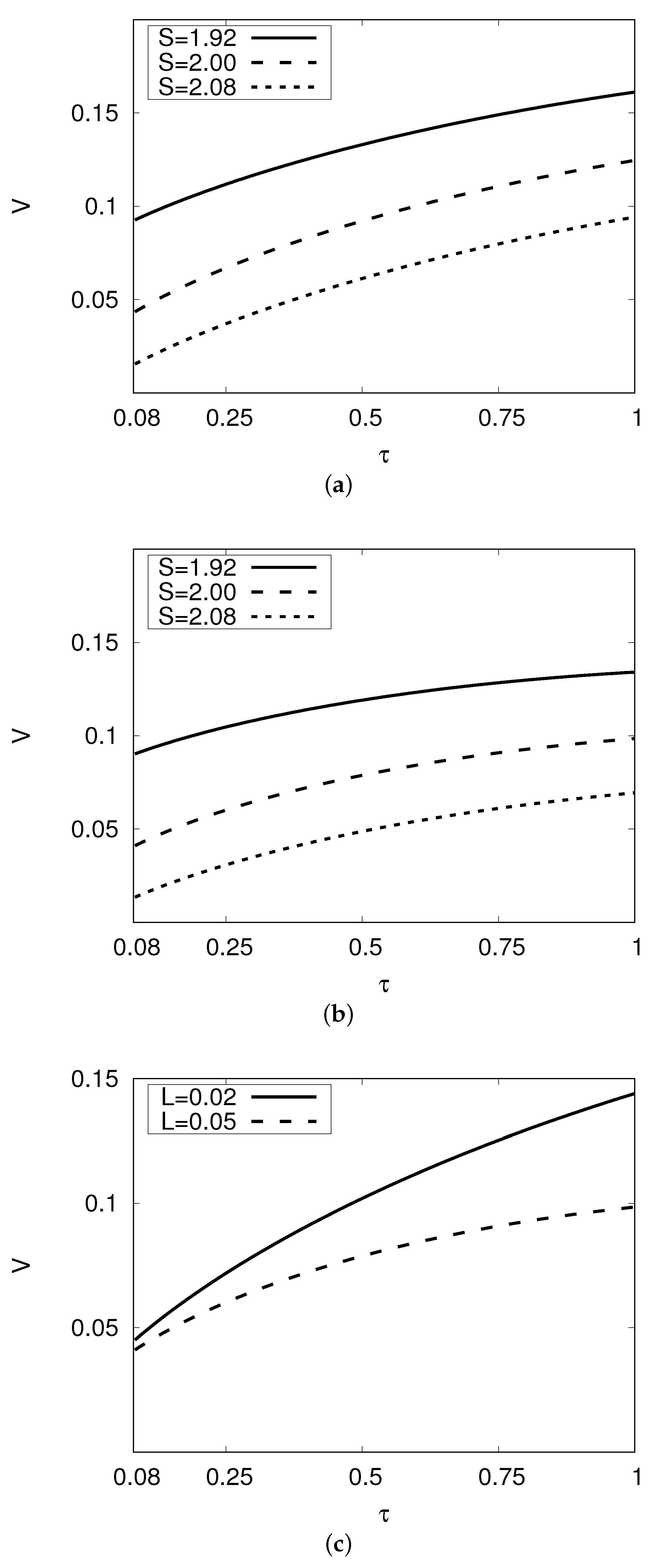
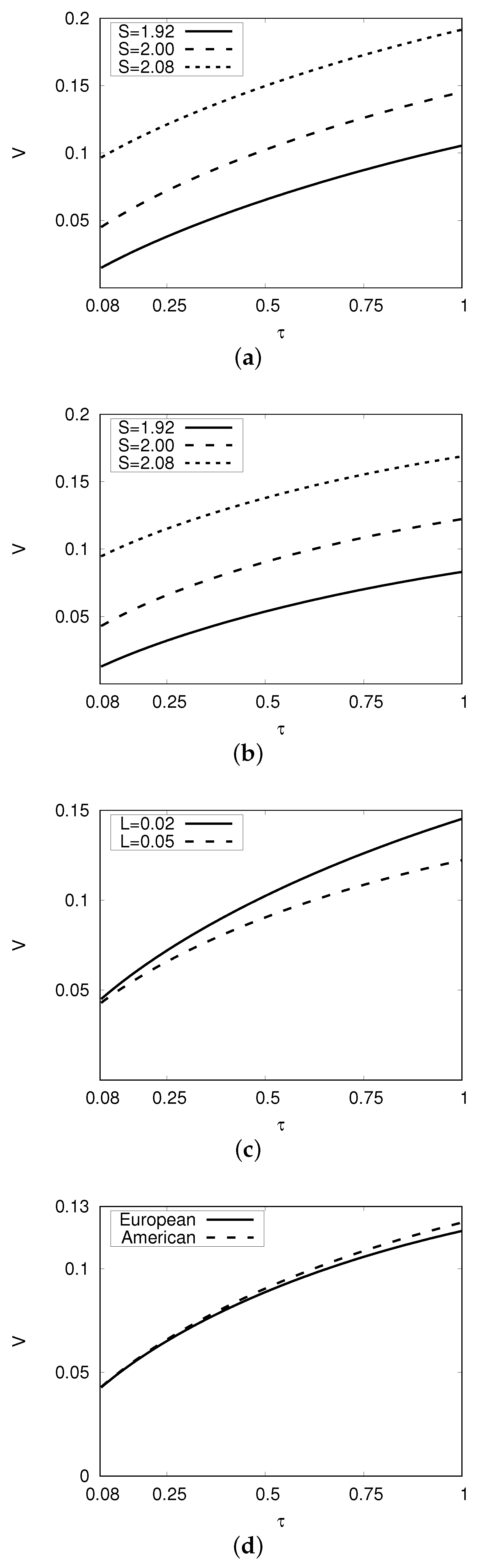
We refer again to Table 1 and Table 3. As with European and American vanilla call/put options, the value of European and American CI call/put options increase/decrease with the underlying price S and all options increase with time-to-expiry $\tau$. In all cases, the increase in installment rate L decreases the option value. This is to be expected, as payments of installments should make the initial premium lower. Hence, the larger L is, the lower the initial premium. See Figure 1, Figure 2, Figure 3 and Figure 4. Note that in Table 3, we used a different value of $q=0.065$ for the American CI put option so as to demonstrate the corresponding behavior of the exercise boundary (Table 4) in that case. However, the values with $q=0.04$ are plotted in Figure 4a–d to compare with the European case.

Figure 1. (a) European CI call (V) values with $L=0.02$, (b) European CI call (V) values with $L=0.05$ and (c) European CI call (V) values with $S=2$ for various expiries ($\tau$). Parameters used: $r=0.05,q=0.04,\sigma =0.2,X=2$.

Figure 2. (a) European CI put (V) values with $L=0.02$, (b) European CI put (V) values with $L=0.05$ and (c) European CI put (V) values with $S=2$ for various expiries ($\tau$). Parameters used: $r=0.05,q=0.04,\sigma =0.2,X=2$.

Figure 3. (a) American CI call (V) values with $L=0.02$, (b) American CI call (V) values with $L=0.05$, (c) American CI call (V) values with $S=2$ and (d) European and American CI call (V) values with $L=0.05$ for various expiries ($\tau$). Parameters used: $r=0.05,q=0.04,\sigma =0.2,X=2$.

Figure 4. (a) American CI put (V) values with $L=0.02$, (b) American CI put (V) values with $L=0.05$, (c) American CI put (V) values with $S=2$ and (d) European and American CI put (V) values with $L=0.05$ for various expiries ($\tau$). Parameters used: $r=0.05,q=0.04,\sigma =0.2,X=2$.

For the critical exit boundary, we can see from Table 2 and Table 4 that $S_z$ and $S_w$ approach $X=2$ as $\tau$ tends to zero. This agrees with the results of Kimura ([8,14]). For the European CI call, for all expiries $\tau$, $S_z\left(\tau \right)<X=2$, as expected, so the option is out-of-the-money when the option is withdrawn. The amount that it is out-of-the money decreases with L, i.e., $|S_z-X|$ decreases with L, so for larger installment payments there are less values of the asset price where it is best to keep paying installments. As a function of $\tau$, for the parameters listed for the call, $S_z$ decreases from $X=2$. However, this may not always be the case, and is discussed a little bit further.

With the European CI put, for all expiries $\tau$, $S_z\left(\tau \right)>X=2$, as expected, so the option is out-of-the-money when the option is withdrawn. Again, the amount that it is out-of-the money decreases with L, i.e., $|X-S_z|$ decreases with L, so for larger installment payments, there are fewer values of the asset price where it is best to keep paying installments. As a function of $\tau$ for the parameters listed for the put, $S_z$ increases from $X=2$.

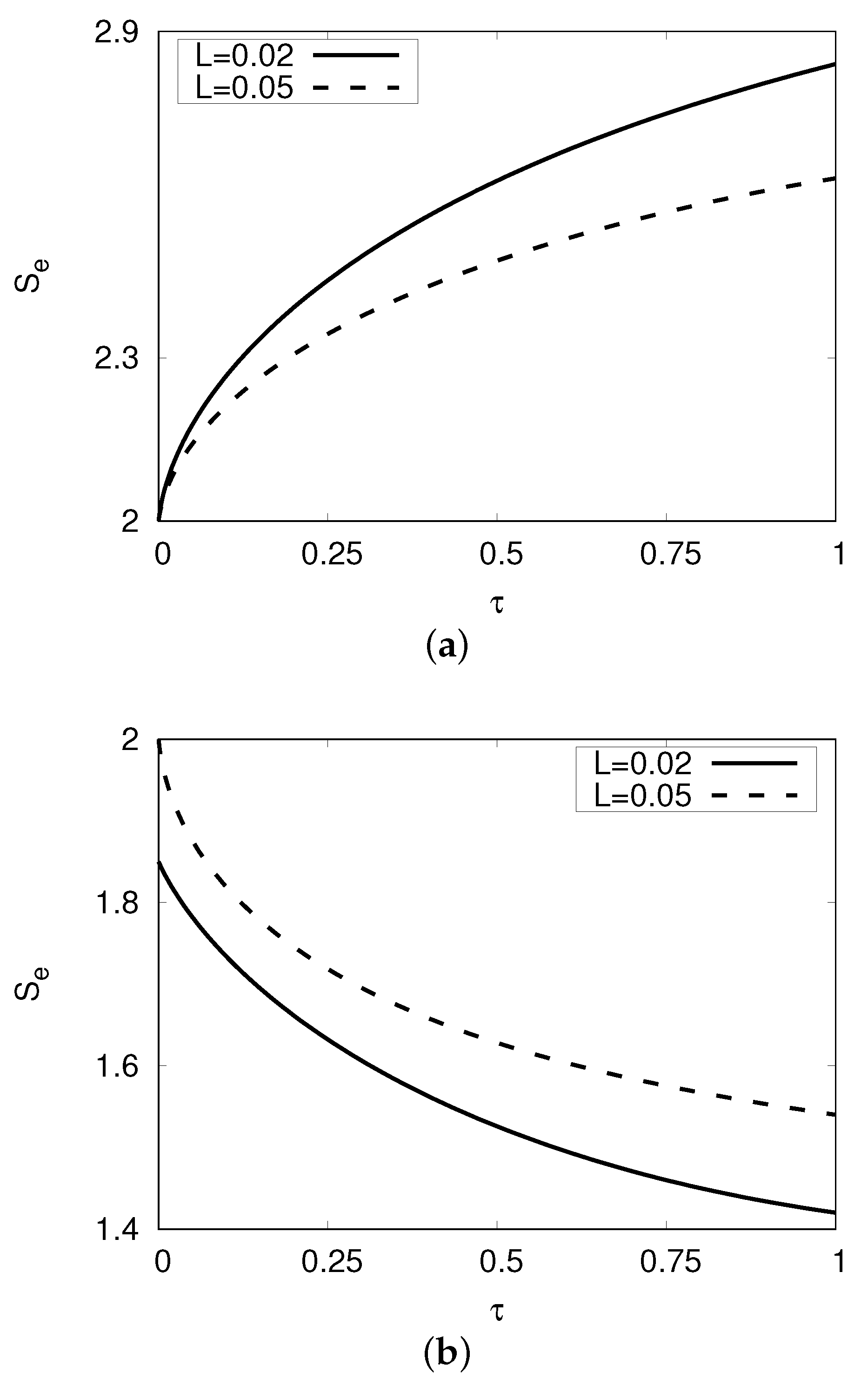
While the exit boundaries for the CI call (put) options in the cases $L=0.02,0.05$ decrease (increase) as a function of time-to-expiry, up to $\tau =1$, it seems unreasonable to believe that the investor would continue to pay installments for increasing out-of-the moneyness for all times-to-expiry. This is even more so the case for larger L. To test this, we used $L=0.2$ and for the European CI call option found that the exit boundary decreased from $X=2$ to 1.83 at $\tau =3/12$, but then increased towards $X=2$, so that at $\tau =1$ it was 1.88. By $\tau =1.5$ it was 1.93. Hence, it is in fact a convex function of $\tau$.

For smaller L, it takes much longer to reach the turning point. For $L=0.05$, $S_z$ slowly decreases with $\tau$ to about a minimum of 1.44 at $\tau =4$, but by $\tau =10$, its value is 1.52.

In a similar way, the exit boundary for the CI put option is concave as a function of $\tau$ so that $|X-S_z|$ increases, then decreases. See Figure 5a,b.

Figure 5. (a) Critical exit $S_z$ values for the European CI call and (b) Critical exit $S_z$ values for the European CI put for various expiries ($\tau$). Parameters used: $r=0.05,q=0.04,\sigma =0.2,X=2$.

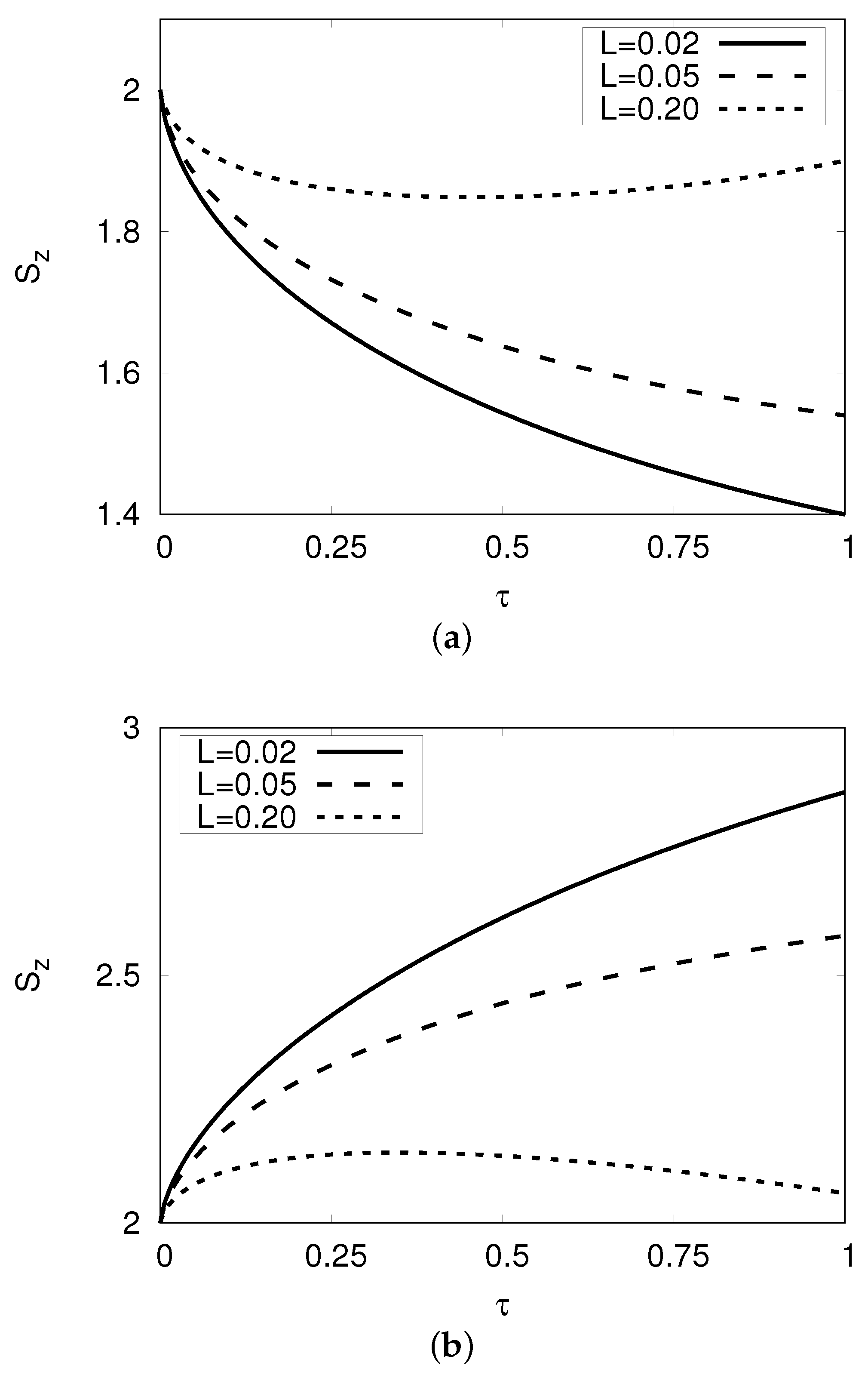
For the exercise boundaries of American CI call options, from Table 4, we see that the results in the limit as $\tau$ tends to zero agree with $S_e\left(0\right)=max\left(\frac{rX-L}{q},X\right)$. When $L=0.02$ and 0.05, we have $S_e$ tending towards $X=2$. Similarly for the exercise boundaries of American CI put options, from Table 4, we see that the results in the limit as $\tau$ tends to zero agree with $S_e\left(0\right)=min\left(\frac{rX+L}{q},X\right)$. When $L=0.02$, we have $S_e$ tending towards 1.846, while for $L=0.05$, $S_e$ tends towards 2 as $\tau$ tends to zero. See Figure 6a,b.

Figure 6. (a) Optimal exercise $S_e$ values for the American CI call and (b) Optimal exercise $S_e$ values for the American CI put for various expiries ($\tau$). Parameters used: $r=0.05,q=0.04,\sigma =0.2,X=2$.

5. Conclusions

Financial contracts that offer reduced upfront premiums are very popular in financial markets. One such contract is the installment option, which allows the investor to pay the premium in installments over the life of the contract, and also allows the investor to exit (or cancel) the contract early if they so desire. In this paper, we have addressed the issue of pricing short-term continuous installment options—both call and put options of both the European and American type. Given that there are currently no exact pricing formulae for these options, this issue is very important. We have formulated accurate and efficient analytical approximations for all these options with short tenor. As the majority of options in the market have expiries of less than 9 months, this is an important development in this field. It was demonstrated that not only did the solutions yield very accurate and efficient results for the option price, but also for the exit stock price boundaries and the exercise boundaries for the American CI options. In the absence of scaling invariance, multiple free boundaries and even single free boundaries are extremely difficult to locate in closed analytical form. Therefore, finding very accurate approximations for them is, we believe, an important achievement. Our results also outperformed the results from Kimura’s method [8]. Further, having analytic approximations, we were able to determine the behavior of the critical boundaries near expiry. The exit boundaries for the European and American CI call and put options close to expiry were found to have levels of moneyness $\theta \sim \sqrt{ln(1/\tau )}$ which do not depend on the parameters $r,q$ and L. However, the early exercise levels of moneyness for the American CI call close to expiry $\sim \sqrt{ln(1/\tau )}$ when $(q-r)X+L>0$ and $\sim \sqrt{\tau }$ when $(q-r)X+L=0$. For the American CI put, the early exercise levels of moneyness $\sim \sqrt{ln(1/\tau )}$ when $(r-q)X+L>0$ and $\sim \sqrt{\tau }$ when $(r-q)X+L=0$.