A New Parameter Choice Strategy for Lavrentiev Regularization Method for Nonlinear Ill-Posed Equations

Abstract

In this paper, we introduced a new source condition and a new parameter-choice strategy which also gives the known best error estimate. To obtain the results we used the assumptions used in earlier studies. Further, we studied the proposed new parameter-choice strategy and applied it to the method (in the finite-dimensional setting) considered in George and Nair (2017).

1. Introduction

Let $\mathcal{H}:D\left(\mathcal{H}\right)\subseteq \mathcal{U}\to \mathcal{U}$ be a nonlinear monotone operator, i.e.,

$$⟨\mathcal{H}\left(v\right)-\mathcal{H}\left(w\right),v-w⟩\ge 0,\forall v,w\in D\left(\mathcal{H}\right),$$

defined on the real Hilbert space $\mathcal{U}$. Here and below $⟨.,.⟩$ and $\parallel .\parallel$, respectively, denote the inner product and corresponding norm in $\mathcal{U};$ $B(u,r)$ and $\overline{B(u,r)}$, respectively, denote open and closed ball in $\mathcal{U}$ with center $u\in \mathcal{U}$ and radius $r>0.$ We are concerned with finite dimensional approximation of the ill-posed equation

$$\mathcal{H}\left(u\right)=y,$$

(1)

which has a solution $\widehat{u}$ for exact data $y.$ However, we have $y^{\delta }\in \mathcal{U}$ for some $\delta >0,$ are the available data, such that

$$\parallel y-y^{\delta }\parallel \le \delta .$$

(2)

Due to the ill-posedness of (1), one has to apply regularization method to obtain an approximation for $\widehat{u}.$ For (1) with monotone $\mathcal{H},$ Lavrentiev regularization (LR) method is widely used (see [1,2,3,4,5,6]). In (LR) method the solution $u_{\alpha }^{\delta }$ of the equation

$$\mathcal{H}\left(u\right)+\alpha (u-u_0)=y^{\delta },$$

(3)

is used as an approximation for $\widehat{u}.$ Here (and below) $u_0$ is an initial approximation of $\widehat{u}$ with $\parallel u_0-\widehat{u}\parallel \le r_0$ for some $r_0>0.$ The solution of (3), with y in place of $y^{\delta }$ is denoted by $u_{\alpha }$, i.e., (cf. [5])

$$\mathcal{H}\left(u_{\alpha }\right)+\alpha (u_{\alpha }-u_0)=y.$$

(4)

Let $u_{\alpha }^{\delta }$ and $u_{\alpha }$ be as in Equations (3) and (4), respectively. Then, we have the following inequalities (cf. [5]).

$$\begin{array}{ccc}\hfill \parallel u_{\alpha }-\widehat{u}{\parallel }^2& \le & ⟨u_0-\widehat{u},u_{\alpha }-\widehat{u}⟩,\hfill \\ \hfill \parallel u_{\alpha }^{\delta }-u_{\alpha }\parallel & \le & \frac{\delta }{\alpha },\hfill \end{array}$$

(5)

and hence,

$$\begin{array}{ccc}\hfill \parallel \widehat{u}-u_{\alpha }^{\delta }\parallel & \le & \parallel \widehat{u}-u_{\alpha }\parallel +\frac{\delta }{\alpha }\hfill \end{array}$$

(6)

and

$$\begin{array}{ccc}\hfill \parallel \widehat{u}-u_{\alpha }\parallel & \le & \parallel \widehat{u}-u_0\parallel .\hfill \end{array}$$

(7)

For proving our result, we assume that, either ${\mathcal{H}}^{\prime }\left(u\right)$ is self-adjoint or ${\mathcal{H}}^{\prime }\left(u\right)$ is positive type, i.e.,

$$\sigma \left({\mathcal{H}}^{\prime }\left(u\right)\right)\subseteq [0,\infty )$$

and

$$\parallel {({\mathcal{H}}^{\prime }\left(u\right)+sI)}^{-1}\parallel \le \frac{c}{s},s>0,\text{for some constant}c>0,u\in \overline{B(u_0,r)}$$

(see [7]). Here and below ${\mathcal{H}}^{\prime }\left(u\right)$ is the Fréchet derivative of $\mathcal{H}\left(u\right)$ (if ${\mathcal{H}}^{\prime }\left(u\right)$ is self-adjoint, then $c=1$).

Remark 1.

If ${\mathcal{H}}^{\prime }\left(u\right)$ is positive type, then

$$\parallel {({\mathcal{H}}^{\prime }\left(u\right)+sI)}^{-1}{\mathcal{H}}^{\prime }\left(u\right)\parallel =\parallel I-s{({\mathcal{H}}^{\prime }\left(u\right)+sI)}^{-1}\parallel \le 1+c.$$

Further as in [8] (Lemma 2.2) one can prove

$$\parallel {({\mathcal{H}}^{\prime }\left(u\right)+sI)}^{-1}{\mathcal{H}}^{\prime }{\left(u\right)}^{\mu }\parallel =O\left(s^{\mu }\right),0\le \mu <1.$$

So, the results in this paper hold for positive type operator ${\mathcal{H}}^{\prime }\left(u\right)$ up to a constant. Therefore, for convenience, hereafter we assume ${\mathcal{H}}^{\prime }(.)$ is self-adjoint.

In earlier studies such as [4,5,6,9,10], the following source condition:

$$u_0-\widehat{u}={\mathcal{H}}^{\prime }{\left(\widehat{u}\right)}^{{\mu }_1}z,\parallel z\parallel \le \rho ,0<{\mu }_1\le 1.$$

(8)

or

$$u_0-\widehat{u}={\mathcal{H}}^{\prime }{\left(u_0\right)}^{{\mu }_2}z,\parallel z\parallel \le \rho ,0<{\mu }_2\le 1$$

(9)

was used to obtain an estimate for $\parallel \widehat{u}-u_{\alpha }\parallel .$ In fact, if the source condition (8) is satisfied, then, we have [5]

$$\parallel \widehat{u}-u_{\alpha }\parallel =O\left({\alpha }^{{\mu }_1}\right)$$

and if (9) is satisfied, then, we have [2]

$$\parallel \widehat{u}-u_{\alpha }\parallel =O\left({\alpha }^{{\mu }_2}\right).$$

In this study, we introduce a new source condition,

$$u_0-\widehat{u}=A^{\nu }z,\parallel z\parallel \le \rho ,0<\nu \le 1,$$

(10)

where $\rho >0$ and $A={\int }_0^1{\mathcal{H}}^{\prime }(\widehat{u}+t(u_0-\widehat{u}))dt.$ We shall use this source condition (10) to obtain a convergence rate for $\parallel \widehat{u}-u_{\alpha }\parallel$ and to introduce a new parameter-choice strategy.

Remark 2.

(a) Note that in a posteriori parameter-choice strategy, the regularization parameter α (depending on δ and $y^{\delta }$) is chosen at the time of computing $u_{\alpha }^{\delta }$ (see [11]). The new source condition (10) is used to choose the parameter α (depending on δ and $y^{\delta }$) and independent of $\nu ,$ before computing $u_{\alpha }^{\delta }$ (see Section 2) and also it gives the best known convergence order (see Remark 4). This is the innovation of our approach.

(b) Notice that, the operator A and $A^{\nu }$ are used to obtain an estimate for $\parallel \widehat{u}-u_{\alpha }\parallel .$ In actual computation of the approximation $u_{n+1,\alpha }^{h,\delta }$ (see Equation (38)) and α (see Section 4) we do not require the operator A or $A^{\nu }.$

The following formula ([12], p. 287) for fractional power of positive type operators $\mathcal{B}$ is used in our analysis.

$$\begin{array}{ccc}\hfill {\mathcal{B}}^{z}x& =& \frac{sin\pi z}{\pi }{\int }_0^{\infty }{\tau }^z\left[{(\mathcal{B}+\tau I)}^{-1}x-\frac{\mathrm{\Theta }\left(\tau \right)}{\tau }x+\dots +{(-1)}^n\frac{\mathrm{\Theta }\left(\tau \right)}{{\tau }^n}{\mathcal{B}}^{n-1}x\right]d\tau \hfill \\ \hfill & & +\frac{sin\pi z}{\pi }\left[\frac{x}{z}-\frac{\mathcal{B}x}{z-1}+\dots +{(-1)}^{n-1}\frac{{\mathcal{B}}^{n-1}x}{z-n+1}\right],x\in \mathcal{U},\hfill \end{array}$$

where

$$\mathrm{\Theta }\left(\varsigma \right)=\left\{\begin{array}{cc}0& \mathrm{if}0\le \varsigma \le 1\\ 1& \mathrm{if}1<\varsigma <\infty \end{array}\right.$$

and z is a complex number such that $0<Rez<n.$

Let $z=\nu ,$ and $\mathcal{B}={\mathcal{H}}^{\prime }(.)$. Then, we have

$${\mathcal{H}}^{\prime }{(.)}^{\nu }x=\frac{sin\pi \left(\nu \right)}{\pi }\left[\frac{x}{\nu }+{\int }_0^{\infty }{\tau }^{\nu }{({\mathcal{H}}^{\prime }(.)+\tau I)}^{-1}xd\tau -{\int }_1^{\infty }\frac{x}{{\tau }^{1-\nu }}d\tau \right].$$

(11)

Note that, if ${\mathcal{H}}^{\prime }(.)$ is self-adjoint, then, A is self-adjoint. Further, suppose ${\mathcal{H}}^{\prime }(.)$ is positive type, then we have

$$\begin{array}{ccc}\hfill {\parallel (A+sI)}^{-1}\parallel & =& \parallel {({\int }_0^1{\mathcal{H}}^{\prime }(\widehat{u}+t(u_0-\widehat{u}))dt+sI)}^{-1}\parallel \hfill \\ & =& \parallel {\left({\int }_0^1({\mathcal{H}}^{\prime }(\widehat{u}+t(u_0-\widehat{u}))+sI)dt\right)}^{-1}\parallel \hfill \\ & \le & {\int }_0^1\parallel {({\mathcal{H}}^{\prime }(\widehat{u}+t(u_0-\widehat{u}))+sI)}^{-1}\parallel dt\hfill \\ & \le & \frac{c}{s},\hfill \end{array}$$

i.e., A is positive type.

Next, we shall prove that (10) implies

$$u_0-\widehat{u}=\left\{\begin{array}{cc}{\mathcal{H}}^{\prime }{\left(u_0\right)}^{{\nu }_1}{\xi }_z,\parallel {\xi }_z\parallel \le {\rho }_0\mathrm{for}& 0<{\nu }_1<\nu <1\\ {\mathcal{H}}^{\prime }\left(u_0\right){\xi }_{z_1},\parallel {\xi }_{z_1}\parallel \le {\rho }_1\mathrm{for}& \nu =1,\end{array}\right.$$

(12)

for some constants ${\rho }_0$ and ${\rho }_1$. For this, we use the standard non-linear assumptions in the literature (cf. [4,13]).

Assumption 1.

For every $u,v\in \overline{B(u_0,r)}$ and $w\in \mathcal{U},$ there exists $k_0>0$ and an element $\mathrm{\Phi }(u,v,w)\in \mathcal{U}$ with

$$[{\mathcal{H}}^{\prime }\left(u\right)-{\mathcal{H}}^{\prime }\left(v\right)]w={\mathcal{H}}^{\prime }\left(v\right)\mathrm{\Phi }(u,v,w)$$

and

$$\parallel \mathrm{\Phi }(u,v,w)\parallel \le k_0\parallel w\parallel \parallel u-v\parallel .$$

Suppose (10) holds for $\nu <1,$ then

$$\begin{array}{ccc}\hfill u_0-\widehat{u}& =& A^{\nu }z\hfill \\ \hfill & =& [A^{\nu }-{\mathcal{H}}^{\prime }{\left(u_0\right)}^{\nu }]z+{\mathcal{H}}^{\prime }{\left(u_0\right)}^{\nu }z\hfill \\ \hfill & =& -\frac{sin\pi \left(\nu \right)}{\pi }{\int }_0^{\infty }{\tau }^{\nu }{({\mathcal{H}}^{\prime }\left(u_0\right)+\tau I)}^{-1}(A-{\mathcal{H}}^{\prime }\left(u_0\right)){(A+\tau I)}^{-1}zd\tau \hfill \\ \hfill & & +{\mathcal{H}}^{\prime }{\left(u_0\right)}^{\nu }z,\hfill \end{array}$$

so by the definition of A and Assumption 1, we have

$$\begin{array}{ccc}\hfill u_0-\widehat{u}& =& [A^{\nu }-{\mathcal{H}}^{\prime }{\left(u_0\right)}^{\nu }]z+{\mathcal{H}}^{\prime }{\left(u_0\right)}^{\nu }z\hfill \\ \hfill & =& -\frac{sin\pi \left(\nu \right)}{\pi }{\int }_0^{\infty }{\tau }^{\nu }{({\mathcal{H}}^{\prime }\left(u_0\right)+\tau I)}^{-1}\hfill \\ & & \times {\int }_0^1({\mathcal{H}}^{\prime }(\widehat{u}+t(u_0-\widehat{u}))-{\mathcal{H}}^{\prime }\left(u_0\right))dt{(A+\tau I)}^{-1}zd\tau \hfill \\ \hfill & & +{\mathcal{H}}^{\prime }{\left(u_0\right)}^{\nu }z\hfill \\ \hfill & =& -\frac{sin\pi \left(\nu \right)}{\pi }{\int }_0^{\infty }{\tau }^{\nu }{({\mathcal{H}}^{\prime }\left(u_0\right)+\tau I)}^{-1}{\mathcal{H}}^{\prime }\left(u_0\right)\hfill \\ \hfill & & \times {\int }_0^1\mathrm{\Phi }(\widehat{u}+t(u_0-\widehat{u}),u_0,{(A+\tau I)}^{-1}z)dtd\tau +{\mathcal{H}}^{\prime }{\left(u_0\right)}^{\nu }z\hfill \\ \hfill & =& {\mathcal{H}}^{\prime }\left(u_0\right)[-\frac{sin\pi \left(\nu \right)}{\pi }{\int }_0^{\infty }{\tau }^{\nu }{({\mathcal{H}}^{\prime }\left(u_0\right)+\tau I)}^{-1}\hfill \\ \hfill & & \times {\int }_0^1\mathrm{\Phi }(\widehat{u}+t(u_0-\widehat{u}),u_0,{(A+\tau I)}^{-1}z)dtd\tau ]+{\mathcal{H}}^{\prime }{\left(u_0\right)}^{\nu }z\hfill \\ \hfill & =& {\mathcal{H}}^{\prime }{\left(u_0\right)}^{{\nu }_1}{\xi }_z,{\nu }_1<\nu ,\hfill \end{array}$$

where ${\xi }_z={\mathcal{H}}^{\prime }{(u_0)}^{1-{\nu }_1}(-\frac{sin\pi (\nu )}{\pi }{\int }_0^{\infty }{\tau }^{\nu }{({\mathcal{H}}^{\prime }(u_0)+\tau I)}^{-1}{\int }_0^1\mathrm{\Phi }(\widehat{u}+t(u_0-\widehat{u}),u_0,{(A+\tau I)}^{-1}$$z)dt)d\tau +{\mathcal{H}}^{\prime }{(u_0)}^{\nu -{\nu }_1}z.$ Further note that

$$\begin{array}{ccc}\hfill \parallel {\xi }_z\parallel & \le & \frac{1}{\pi }\parallel \left({\int }_0^{\infty }{\mathcal{H}}^{\prime }{\left(u_0\right)}^{1-{\nu }_1}{\tau }^{\nu }{({\mathcal{H}}^{\prime }\left(u_0\right)+\tau I)}^{-1}\right.\hfill \\ \hfill & & \left.\times {\int }_0^1\mathrm{\Phi }(\widehat{u}+t(u_0-\widehat{u}),u_0,{(A+\tau I)}^{-1}z)dt\right)d\tau \parallel +\parallel {\mathcal{H}}^{\prime }{\left(u_0\right)}^{\nu -{\nu }_1}z\parallel \hfill \\ & \le & \frac{1}{\pi }[{\int }_0^1{\tau }^{\nu }\parallel {\mathcal{H}}^{\prime }{\left(u_0\right)}^{1-{\nu }_1}{({\mathcal{H}}^{\prime }\left(u_0\right)+\tau I)}^{-1}\parallel k_0\frac{\parallel u_0-\widehat{u}\parallel }{2}\parallel {(A+\tau I)}^{-1}z\parallel d\tau \hfill \\ & & +{\int }_1^{\infty }{\tau }^{\nu }\parallel {\mathcal{H}}^{\prime }{\left(u_0\right)}^{1-{\nu }_1}{({\mathcal{H}}^{\prime }\left(u_0\right)+\tau I)}^{-1}\parallel k_0\frac{\parallel u_0-\widehat{u}\parallel }{2}\parallel {(A+\tau I)}^{-1}z\parallel d\tau ]\hfill \\ & & +\parallel {\mathcal{H}}^{\prime }{\left(u_0\right)}^{\nu -{\nu }_1}\parallel \rho \hfill \\ & \le & \frac{1}{\pi }[{\int }_0^1{\tau }^{\nu -{\nu }_1-1}d\tau k_0\frac{\parallel u_0-\widehat{u}\parallel }{2}\parallel z\parallel \hfill \\ & & +\parallel {\mathcal{H}}^{\prime }{\left(u_0\right)}^{1-{\nu }_1}\parallel {\int }_1^{\infty }{\tau }^{\nu -2}d\tau k_0\frac{\parallel u_0-\widehat{u}\parallel }{2}\parallel z\parallel ]+\parallel {\mathcal{H}}^{\prime }{\left(u_0\right)}^{\nu -{\nu }_1}\parallel \rho \hfill \\ & \le & \frac{1}{\pi }\left[\frac{1}{\nu -{\nu }_1}+\frac{\parallel {\mathcal{H}}^{\prime }{\left(u_0\right)}^{1-{\nu }_1}\parallel }{1-\nu }\right]k_0\frac{r_0}{2}\rho +\parallel {\mathcal{H}}^{\prime }{\left(u_0\right)}^{\nu -{\nu }_1}\parallel \rho :={\rho }_0.\hfill \end{array}$$

Suppose

$$\begin{array}{ccc}\hfill u_0-\widehat{u}& =& Az\hfill \\ & =& [A-{\mathcal{H}}^{\prime }\left(u_0\right)+{\mathcal{H}}^{\prime }\left(u_0\right)]z\hfill \\ & =& [{\int }_0^1({\mathcal{H}}^{\prime }(\widehat{u}+t(u_0-\widehat{u}))-{\mathcal{H}}^{\prime }\left(u_0\right))dt+{\mathcal{H}}^{\prime }\left(u_0\right)]z\hfill \\ & =& {\mathcal{H}}^{\prime }\left(u_0\right)[{\int }_0^1\mathrm{\Phi }(\widehat{u}+t(u_0-\widehat{u}),u_0,z)dt+z]\hfill \\ & =& {\mathcal{H}}^{\prime }\left(u_0\right){\xi }_{z_1},\hfill \end{array}$$

where ${\xi }_{z_1}={\int }_0^1\mathrm{\Phi }(\widehat{u}+t(u_0-\widehat{u}),u_0,z)dt+z.$ Observe that

$$\parallel {\xi }_{z_1}\parallel \le (k_0\frac{\parallel \widehat{u}-u_0\parallel }{2}+1)\parallel z\parallel \le (\frac{k_0{r}_0}{2}+1)\rho ={\rho }_1.$$

So $u_0-\widehat{u}=Az$ implies $u_0-\widehat{u}={\mathcal{H}}^{\prime }\left(u_0\right){\xi }_{z_1},\parallel {\xi }_{z_1}\parallel \le {\rho }_1$ i.e., (10) implies (12). Similarly one can show that (10) implies

$$u_0-\widehat{u}=\left\{\begin{array}{cc}{\mathcal{H}}^{\prime }{\left(\widehat{u}\right)}^{{\nu }_1}{\xi }_z,\parallel {\xi }_z\parallel \le {\rho }_2\mathrm{for}& 0<{\nu }_1<\nu <1\\ {\mathcal{H}}^{\prime }\left(\widehat{u}\right){\xi }_{z_1},\parallel {\xi }_{z_1}\parallel \le {\rho }_1\mathrm{for}& \nu =1,\end{array}\right.$$

for some constant ${\rho }_2.$ Throughout the paper, we use the relation (Fundamental Theorem of Integration),

$$\mathcal{H}\left(u\right)-\mathcal{H}\left(x\right)=\left[{\int }_0^1{\mathcal{H}}^{\prime }(x+t(u-x))dt\right](u-x)$$

for all x and u in a ball contained in $D\left(\mathcal{H}\right).$

Remark 3.

In general, it is believed that (see [5]) a priori parameter-choice strategy is not a good strategy to choose α since the choice is depending on the unknown $\nu .$ In this study, we introduce a new parameter-choice strategy which is not depending on unknown ν and gives the best known convergence order $O({\delta }^{\frac{\nu }{\nu +1}}).$

In some recent papers, the first author and his collaborators considered iterative methods [14,15] for obtaining stable approximate solutions for (3) (see [8,16]). In most of the iterative methods Fréchet derivative of the operator involved is used. In [10], Semenova considered the iterative method defined for fixed $\alpha ,\delta ,$ by

$$u_{n+1,\alpha }^{\delta }=u_{n,\alpha }^{\delta }-\gamma [\mathcal{H}\left(u_{n,\alpha }^{\delta }\right)+\alpha (u_{n,\alpha }^{\delta }-u_0)-y^{\delta }].$$

(13)

Note that, the above iterative method is derivative-free. Convergence analysis in [10] is based on the assumption that $\mathcal{H}$ is Lipschitz continuous and the Lipschitz constant R satisfies

$$0<\gamma <min\left\{\frac{1}{\alpha },\frac{2\alpha }{{\alpha }^2+R^2}\right\},$$

(14)

where $\gamma$ is a constant. Contraction mapping arguments are used to prove the convergence in [10].

In [16], George and Nair considered the method (13), but with $\beta$ independent on the regularization parameter $\alpha$ and the Lipschitz constant $R,$ instead of $\gamma .$ The source condition on $u_0-\widehat{u}$ in [16] depends on the known $u_0$ and the analysis in [16] is not based on the contraction mapping arguments as in [10].

The purpose of this paper is threefold: (1) introduce a new source condition, (2) introduce a new parameter-choice strategy, and (3) apply the parameter-choice strategy to the (finite–dimensional setting of the) method in [16].

The remainder of the paper is organized as follows. In Section 2, we present the error bounds under the source condition (10) and a new parameter-choice strategy. In Section 3, we present the finite dimensional realization of method (13). In Section 4, we present the finite dimensional realization of (10). Section 5 contains the numerical example and the conclusion is given in Section 6.

2. Error Bounds under (10) and a New Parameter Choice Strategy

First we obtain an estimate for $\parallel \widehat{u}-u_{\alpha }\parallel$ using (10).

Theorem 1.

Let $\frac{3}{2}{k}_0{r}_0<1,$ Assumption 1 and (10) be satisfied. Then,

$$\parallel \widehat{u}-u_{\alpha }\parallel \le \frac{2+k_0{r}_0}{3-2k_0{r}_0}{\alpha }^{\nu }\parallel z\parallel .$$

Proof. 

Since $\mathcal{H}\left(\widehat{u}\right)=y$ and $\mathcal{H}\left(u_{\alpha }\right)+\alpha (u_{\alpha }-u_0)=y,$ we have

$$\mathcal{H}\left(u_{\alpha }\right)-\mathcal{H}\left(\widehat{u}\right)+\alpha (u_{\alpha }-u_0)=0,$$

i.e.,

$$\mathcal{H}\left(u_{\alpha }\right)-\mathcal{H}\left(\widehat{u}\right)+\alpha (u_{\alpha }-\widehat{u})=\alpha (u_0-\widehat{u}),$$

(15)

or

$$(M_{\alpha }+\alpha I)(u_{\alpha }-\widehat{u})=\alpha (u_0-\widehat{u}),$$

(16)

where

$$M_{\alpha }={\int }_0^1{\mathcal{H}}^{\prime }(\widehat{u}+t(u_{\alpha }-\widehat{u}))dt.$$

Again (16) can be written as

$$(A_0+\alpha I)(u_{\alpha }-\widehat{u})=(A_0-M_{\alpha })(u_{\alpha }-\widehat{u})+\alpha (u_0-\widehat{u}),$$

where $A_0={\mathcal{H}}^{\prime }\left(u_0\right).$ Thus, we have

$$\begin{array}{ccc}\hfill u_{\alpha }-\widehat{u}& =& -{(A_0+\alpha I)}^{-1}(M_{\alpha }-A_0)(u_{\alpha }-\widehat{u})+\alpha {(A_0+\alpha I)}^{-1}(u_0-\widehat{u})\hfill \\ & =& -{(A_0+\alpha I)}^{-1}\left[{\int }_0^1[{\mathcal{H}}^{\prime }(\widehat{u}+t(u_{\alpha }-\widehat{u}))-{\mathcal{H}}^{\prime }\left(u_0\right)]\right](u_{\alpha }-\widehat{u})dt\hfill \\ & & +\alpha {(A_0+\alpha I)}^{-1}(u_0-\widehat{u})\hfill \\ & =& -{(A_0+\alpha I)}^{-1}{A}_0{\int }_0^1\mathrm{\Phi }\left(\widehat{u}+t(u_{\alpha }-\widehat{u}),u_0,u_{\alpha }-\widehat{u}\right)dt\hfill \\ & & +\alpha {(A_0+\alpha I)}^{-1}(u_0-\widehat{u})\hfill \end{array}$$

and hence

$$\begin{array}{ccc}\hfill \parallel u_{\alpha }-\widehat{u}\parallel & \le & k_0[\frac{\parallel u_{\alpha }-\widehat{u}\parallel }{2}+\parallel \widehat{u}-u_0\parallel ]\parallel u_{\alpha }-\widehat{u}\parallel \hfill \\ & & +\parallel \alpha {(A_0+\alpha I)}^{-1}(u_0-\widehat{u})\parallel \hfill \\ & \le & \frac{3}{2}{k}_0{r}_0\parallel u_{\alpha }-\widehat{u}{\parallel +\alpha \parallel (A+\alpha I)}^{-1}(u_0-\widehat{u})\parallel \mathrm{by}\left(7\right)\hfill \\ & & +\alpha \parallel [{(A_0+\alpha I)}^{-1}-{(A+\alpha I)}^{-1}](u_0-\widehat{u})\parallel \hfill \\ & \le & \frac{3}{2}{k}_0{r}_0\parallel u_{\alpha }-\widehat{u}{\parallel +\alpha \parallel (A+\alpha I)}^{-1}(u_0-\widehat{u})\parallel \hfill \\ & & +\parallel {(A_0+\alpha I)}^{-1}(A-A_0)\alpha {(A+\alpha I)}^{-1}(u_0-\widehat{u})\parallel \hfill \\ & \le & \frac{3}{2}{k}_0{r}_0\parallel u_{\alpha }-\widehat{u}{\parallel +\alpha \parallel (A+\alpha I)}^{-1}(u_0-\widehat{u})\parallel \hfill \\ & & +\parallel A_0{(A_0+\alpha I)}^{-1}{\int }_0^1\mathrm{\Phi }(\widehat{u}+t(u_0-\widehat{u}),u_0,\alpha {(A+\alpha I)}^{-1}(u_0-\widehat{u}))dt\parallel \hfill \\ & \le & \frac{3}{2}{k}_0{r}_0\parallel u_{\alpha }-\widehat{u}{\parallel +\alpha \parallel (A+\alpha I)}^{-1}(u_0-\widehat{u})\parallel \hfill \\ & & +\frac{k_0{r}_0}{2}\parallel \alpha {(A+\alpha I)}^{-1}(u_0-\widehat{u})\parallel \hfill \end{array}$$

i.e.,

$$\begin{array}{ccc}\hfill \left(1-\frac{3}{2}{k}_0{r}_0\right)\parallel u_{\alpha }-\widehat{u}\parallel & \le & (1+\frac{k_0{r}_0}{2})\parallel \alpha {(A+\alpha I)}^{-1}(u_0-\widehat{u})\parallel \hfill \\ \hfill \frac{2-3k_0{r}_0}{2+k_0{r}_0}\parallel \widehat{u}-u_{\alpha }\parallel & \le & {\parallel \alpha (A+\alpha I)}^{-1}{A}^{\nu }z\parallel \mathrm{by}\left(10\right)\hfill \\ \hfill & \le & \underset{\lambda \in \sigma \left(A\right)}{sup}\left|\frac{\alpha {\lambda }^{\nu }}{\lambda +\alpha }\right|\parallel z\parallel \hfill \\ \hfill & \le & {\alpha }^{\nu }\parallel z\parallel .\hfill \end{array}$$

(17)

□

Theorem 2.

Suppose Assumption 1 and (10) hold. Then,

$$\parallel u_{\alpha }^{\delta }-\widehat{u}\parallel \le max\{1,\frac{2+k_0{r}_0}{3-2k_0{r}_0}\parallel z\parallel \}(\frac{\delta }{\alpha }+{\alpha }^{\nu }).$$

In particular, if $\alpha ={\delta }^{\frac{1}{\nu +1}},$ then

$$\parallel u_{\alpha }^{\delta }-\widehat{u}\parallel =O\left({\delta }^{\frac{\nu }{\nu +1}}\right).$$

Proof. 

Follows from (6) and Theorem 1. □

Remark 4.

Note that the best value for $\frac{\delta }{\alpha }+{\alpha }^{\nu }$ is attained when $\frac{\delta }{\alpha }={\alpha }^{\nu }$, i.e., $\alpha ={\delta }^{\frac{1}{\nu +1}},$ and in this case the optimal order is $O\left({\delta }^{\frac{\nu }{\nu +1}}\right).$ However, the above choice of α is depending on the unknown $\nu .$ In view of this, our aim is to choose α (not depending on ν), so that we obtain $\parallel u_{\alpha }^{\delta }-\widehat{u}\parallel =O\left({\delta }^{\frac{\nu }{\nu +1}}\right).$

A New Parameter Choice Strategy

For $u\in \mathcal{U},$ define

$$\varphi (\alpha ,u):=\parallel {\alpha }^2{(A_0+\alpha I)}^{-2}(\mathcal{H}\left(u_0\right)-u)\parallel ,$$

(18)

where $A_0={\mathcal{H}}^{\prime }\left(u_0\right).$

Theorem 3.

For each $u\in \mathcal{U},$ and $\alpha >0$ the function $\alpha \to \varphi (\alpha ,u)$ is continuous, monotonically increasing and

$$\underset{\alpha \to 0}{lim}\varphi (\alpha ,u)=0\mathrm{and}\underset{\alpha \to \infty }{lim}\varphi (\alpha ,u)=\parallel \mathcal{H}\left(u_0\right)-u\parallel .$$

Proof. 

Note that

$$\varphi {(\alpha ,u)}^2={\int }_0^{\parallel A_0\parallel }{\left(\frac{\alpha }{\lambda +\alpha }\right)}^{4}d{\parallel E_{\lambda }(\mathcal{H}\left(u_0\right)-u)\parallel }^2,$$

where $E_{\lambda }$ is the spectral family of $A_0.$ Note that for each $\lambda >0,$

$$\alpha ⟶{\left(\frac{\alpha }{\lambda +\alpha }\right)}^4$$

is strictly increasing and satisfies ${lim}_{\alpha ⟶0}{\left(\frac{\alpha }{\lambda +\alpha }\right)}^4=0$ and ${lim}_{\alpha ⟶\infty }{\left(\frac{\alpha }{\lambda +\alpha }\right)}^4=1.$ Hence, by Dominated Convergence Theorem $\varphi (\alpha ,u)$ is strictly increasing, continuous, ${lim}_{\alpha \to 0}\varphi (\alpha ,u)$$=0\mathrm{and}{lim}_{\alpha \to \infty }\varphi (\alpha ,u)=\parallel \mathcal{H}\left(u_0\right)-u\parallel .$ □

In addition to (2), we assume that

$$c\delta \le \parallel \mathcal{H}\left(u_0\right)-y^{\delta }\parallel ,$$

(19)

for some $c>1.$ The following theorem is a consequence of the intermediate value theorem.

Theorem 4.

Let $y^{\delta }$ satisfies (2) and (19). Then,

$$\varphi (\alpha ,y^{\delta })=c\delta$$

(20)

has a unique solution $\alpha .$

Next, we shall show that if $\alpha =\alpha (\delta ,u_0)$ satisfies (10) and (20) hold, then $\parallel \widehat{u}-u_{\alpha }\parallel$$=O\left({\delta }^{\frac{\nu }{\nu +1}}\right).$ Our proof is based on the following moment inequality for positive type operator B (see [12], p. 290)

$$\parallel B^{u}x\parallel \le \parallel B^v{x\parallel }^{\frac{u}{v}}{\parallel x\parallel }^{1-\frac{u}{v}},0\le u\le v.$$

(21)

Theorem 5.

Let $\frac{3}{2}{k}_0{r}_0<1,$ Assumption 1 and (10) be satisfied. Let $\alpha =\alpha (\delta ,u_0)$ be the solution of (20). Then,

$$\parallel \widehat{u}-u_{\alpha }\parallel \le O\left({\delta }^{\frac{\nu }{\nu +1}}\right).$$

Proof. 

By taking $B=\alpha {(A+\alpha I)}^{-1}A$ and $x={\alpha }^{1-\nu }{(A+\alpha I)}^{-(1-\nu )}z$ in (17) and then using (21) with $u=\nu ,$$v=1+\nu ,$ we have

$$\begin{array}{ccc}\hfill \frac{2-3k_0{r}_0}{2+k_0{r}_0}\parallel \widehat{u}-u_{\alpha }\parallel & \le & \parallel B^{\nu }x\parallel \hfill \\ \hfill & \le & \parallel B^{1+\nu }{x\parallel }^{\frac{\nu }{1+\nu }}{\parallel x\parallel }^{\frac{1}{1+\nu }}\hfill \\ \hfill & =& \parallel {\alpha }^2{(A+\alpha I)}^{-2}{A}^{1+\nu }{z\parallel }^{\frac{\nu }{1+\nu }}{\parallel z\parallel }^{\frac{1}{1+\nu }}\hfill \\ \hfill & =& \parallel {\alpha }^2{(A+\alpha I)}^{-2}A(u_0-\widehat{u}){\parallel }^{\frac{\nu }{1+\nu }}{\parallel z\parallel }^{\frac{1}{1+\nu }}\hfill \\ \hfill & =& \parallel {\alpha }^2{(A+\alpha I)}^{-2}(\mathcal{H}\left(u_0\right)-y){\parallel }^{\frac{\nu }{1+\nu }}{\parallel z\parallel }^{\frac{1}{1+\nu }}\hfill \\ \hfill & \le & \left(\parallel {\alpha }^2{(A+\alpha I)}^{-2}(\mathcal{H}\left(u_0\right)-y^{\delta })\parallel \right.\hfill \\ \hfill & & +{\left.\parallel {\alpha }^2{(A+\alpha I)}^{-2}(y^{\delta }-y)\parallel \right)}^{\frac{\nu }{1+\nu }}{\parallel z\parallel }^{\frac{1}{1+\nu }}\hfill \\ \hfill & =& {({\mathcal{B}}_1+\delta )}^{\frac{\nu }{1+\nu }}{\parallel z\parallel }^{\frac{1}{1+\nu }}\hfill \end{array}$$

(22)

where ${\mathcal{B}}_1=\parallel {\alpha }^2{(A+\alpha I)}^{-2}(\mathcal{H}\left(u_0\right)-y^{\delta })\parallel$ and we used the inequality,

$$\parallel {\alpha }^2{(A+\alpha I)}^{-2}(y^{\delta }-y)\parallel \le \delta .$$

We have,

$$\begin{array}{ccc}\hfill {\mathcal{B}}_1& =& \parallel {\alpha }^2{(A+\alpha I)}^{-2}(\mathcal{H}\left(u_0\right)-y^{\delta })\parallel \hfill \\ \hfill & =& \parallel {\alpha }^2[{(A+\alpha I)}^{-2}-{(A_0+\alpha I)}^{-2}](\mathcal{H}\left(u_0\right)-y^{\delta })\hfill \\ \hfill & & +{\alpha }^2{(A_0+\alpha I)}^{-2}(\mathcal{H}\left(u_0\right)-y^{\delta })\parallel \hfill \\ \hfill & \le & \parallel {\alpha }^2[{(A+\alpha I)}^{-2}-{(A_0+\alpha I)}^{-2}](\mathcal{H}\left(u_0\right)-y^{\delta })\parallel \hfill \\ \hfill & & +\parallel {\alpha }^2{(A_0+\alpha I)}^{-2}(\mathcal{H}\left(u_0\right)-y^{\delta })\parallel \hfill \\ \hfill & =:& {\mathcal{D}}_1+\varphi (\alpha ,y^{\delta })\hfill \end{array}$$

(23)

where ${\mathcal{D}}_1=\parallel {\alpha }^2[{(A+\alpha I)}^{-2}-{(A_0+\alpha I)}^{-2}](\mathcal{H}\left(u_0\right)-y^{\delta })\parallel .$ Let $w={\alpha }^2{(A_0+\alpha I)}^{-2}(\mathcal{H}\left(u_0\right)$$-y^{\delta }).$ Note that,

$$\begin{array}{ccc}\hfill {\mathcal{D}}_1& =& \parallel {\alpha }^2[{(A+\alpha I)}^{-2}-{(A_0+\alpha I)}^{-2}](\mathcal{H}\left(u_0\right)-y^{\delta })\parallel \hfill \\ \hfill & =& {\parallel (A+\alpha I)}^{-2}[A_0^2-A^2+2\alpha (A_0-A)]w\parallel \hfill \\ \hfill & =& {\parallel (A+\alpha I)}^{-2}[(A+A_0)+2\alpha I](A_0-A)w\parallel \hfill \\ \hfill & =& {\parallel (A+\alpha I)}^{-2}[A_0-A+2A+2\alpha I](A_0-A)w\parallel \hfill \\ \hfill & =& \parallel {\left[{(A+\alpha I)}^{-1}(A_0-A)\right]}^{2}w+2{(A+\alpha I)}^{-1}(A_0-A)w\parallel \hfill \\ \hfill & \le & {(\parallel \mathrm{\Gamma }\parallel }^2+2\parallel \mathrm{\Gamma }\parallel )\parallel w\parallel ={(\parallel \mathrm{\Gamma }\parallel }^2+2\parallel \mathrm{\Gamma }\parallel )\varphi (\alpha ,y^{\delta }),\hfill \end{array}$$

(24)

where $\mathrm{\Gamma }={(A+\alpha I)}^{-1}(A_0-A).$ By Assumption 1, we obtain

$$\begin{array}{ccc}\hfill \parallel \mathrm{\Gamma }x\parallel & \le & \parallel [{(A+\alpha I)}^{-1}-{(A_0+\alpha I)}^{-1}](A_0-A)x\parallel \hfill \\ \hfill & & +\parallel {(A_0+\alpha I)}^{-1}(A_0-A)x\parallel \hfill \\ \hfill & =& \parallel {(A_0+\alpha I)}^{-1}[A_0-A]{(A+\alpha I)}^{-1}(A_0-A)x\parallel \hfill \\ \hfill & & +\parallel {(A_0+\alpha I)}^{-1}(A_0-A)x\parallel \hfill \\ \hfill & \le & \parallel {(A_0+\alpha I)}^{-1}{A}_0\hfill \\ \hfill & & \times {\int }_0^1\mathrm{\Phi }(\widehat{u}+t(u_0-\widehat{u}),u_0,{(A+\alpha I)}^{-1}(A_0-A)x)dt\parallel \hfill \\ \hfill & & +\parallel {(A_0+\alpha I)}^{-1}{A}_0{\int }_0^1\mathrm{\Phi }((\widehat{u}+t(u_0-\widehat{u}),u_0,x)dt\parallel \hfill \\ \hfill & \le & \frac{k_0{r}_0}{2}\parallel \mathrm{\Gamma }x\parallel +\frac{k_0{r}_0}{2}\parallel x\parallel ,\hfill \end{array}$$

i.e.,

$$(1-\frac{k_0{r}_0}{2})\parallel \mathrm{\Gamma }x\parallel \le k_0{r}_0\parallel x\parallel ,$$

(25)

and hence

$${\mathcal{B}}_1\le [\frac{2k_0{r}_0}{2-k_0{r}_0}(\frac{2k_0{r}_0}{2-k_0{r}_0}+2)+1]\varphi (\alpha ,y^{\delta })=O\left(\delta \right).$$

(26)

The result now follows from (22)–(26). □

Theorem 6.

Suppose Assumption 1 and (10) hold and if $\alpha =\alpha (\delta ,u_0)$ is chosen as a solution of (20). Then,

$$\frac{\delta }{\alpha }=O\left({\delta }^{\frac{\nu }{\nu +1}}\right).$$

Proof. 

By (20), we have

$$\begin{array}{ccc}\hfill c\delta & =& \parallel {\alpha }^2{(A_0+\alpha I)}^{-2}(\mathcal{H}\left(u_0\right)-y^{\delta })\parallel \hfill \\ \hfill & \le & \parallel {\alpha }^2{(A_0+\alpha I)}^{-2}(\mathcal{H}\left(u_0\right)-y)\parallel \hfill \\ \hfill & & +\parallel {\alpha }^2{(A_0+\alpha I)}^{-2}(y-y^{\delta }))\parallel \hfill \\ \hfill & \le & \parallel {\alpha }^2{(A_0+\alpha I)}^{-2}(\mathcal{H}\left(u_0\right)-y)\parallel +\delta ,\hfill \end{array}$$

so

$$\begin{array}{ccc}\hfill (c-1)\delta & \le & \parallel {\alpha }^2\left[{(A_0+\alpha I)}^{-2}-{(A+\alpha I)}^{-2}\right](\mathcal{H}\left(u_0\right)-y)\parallel \hfill \\ \hfill & & +\parallel {\alpha }^2{(A+\alpha I)}^{-2}(\mathcal{H}\left(u_0\right)-y)\parallel \hfill \\ \hfill & =& \parallel {(A_0+\alpha I)}^{-2}\left[{(A+\alpha I)}^2-{(A_0+\alpha I)}^2\right]\hfill \\ \hfill & & \times {\alpha }^2{(A+\alpha I)}^{-2}(\mathcal{H}\left(u_0\right)-y)\parallel \hfill \\ \hfill & & +\parallel {\alpha }^2{(A+\alpha I)}^{-2}(\mathcal{H}\left(u_0\right)-y)\parallel .\hfill \end{array}$$

(27)

Let $w_1={\alpha }^2{(A+\alpha I)}^{-2}(\mathcal{H}\left(u_0\right)-y).$ Then, similar to (24), we have

$$\begin{array}{ccc}\hfill (c_1-1)\delta & \le & (\parallel {\mathrm{\Gamma }}_1{\parallel }^2+2\parallel {\mathrm{\Gamma }}_1\parallel +1)\parallel w_1\parallel ,\hfill \end{array}$$

(28)

where ${\mathrm{\Gamma }}_1={(A_0+\alpha I)}^{-1}(A-A_0).$ Note that,

$$\begin{array}{ccc}\hfill \parallel {\mathrm{\Gamma }}_{1}x\parallel & =& \parallel {(A_0+\alpha I)}^{-1}(A-A_0)x\parallel \hfill \\ & =& \parallel {(A_0+\alpha I)}^{-1}{A}_0{\int }_0^1\mathrm{\Phi }(\widehat{u}+t(u_0-\widehat{u}),u_0,x)dt\parallel \hfill \\ & \le & \frac{k_0}{2}\parallel u_0-\widehat{u}\parallel \parallel x\parallel \hfill \\ & \le & \frac{k_0{r}_0}{2}\parallel x\parallel ,\hfill \end{array}$$

so

$$\parallel {\mathrm{\Gamma }}_1\parallel \le \frac{k_0{r}_0}{2}.$$

(29)

Therefore, by (10), (28) and (29), we have

$$\begin{array}{cc}\hfill (c-1)\delta & \le \left[{\left(\frac{k_0{r}_0}{2}\right)}^2+k_0{r}_0+1\right]\parallel w_1\parallel \hfill \\ \hfill & =\left[{\left(\frac{k_0{r}_0}{2}\right)}^2+k_0{r}_0+1\right]\parallel {\alpha }^2{(A+\alpha I)}^{-2}A(u_0-\widehat{u})\parallel \hfill \\ \hfill & =\left[{\left(\frac{k_0{r}_0}{2}\right)}^2+k_0{r}_0+1\right]\parallel {\alpha }^2{(A+\alpha I)}^{-2}{A}^{1+\nu }z\parallel \hfill \\ \hfill & \le \left[{\left(\frac{k_0{r}_0}{2}\right)}^2+k_0{r}_0+1\right]\parallel {\alpha }^2{(A+\alpha I)}^{-1}{A}^{\nu }z\parallel \hfill \\ \hfill & \le \left[{\left(\frac{k_0{r}_0}{2}\right)}^2+k_0{r}_0+1\right]{\alpha }^{1+\nu }\parallel z\parallel ,\hfill \end{array}$$

or

$${\alpha }^{1+\nu }\ge \frac{c-1}{\left[{\left(\frac{k_0{r}_0}{2}\right)}^2+k_0{r}_0+1\right]\parallel z\parallel }\delta .$$

(30)

Thus,

$$\frac{\delta }{\alpha }={\delta }^{\frac{\nu }{\nu +1}}{\left(\frac{\delta }{{\alpha }^{\nu +1}}\right)}^{\frac{1}{\nu +1}}=O\left({\delta }^{\frac{\nu }{\nu +1}}\right).$$

□

Combining Theorems 5 and 6, we obtain:

Theorem 7.

Let Assumption 1 and (10) be satisfied and let $\alpha =\alpha (\delta ,u_0)$ be the solution of (20). Then,

$$\parallel u_{\alpha }^{\delta }-\widehat{u}\parallel =O\left({\delta }^{\frac{\nu }{\nu +1}}\right).$$

In [16], the following estimates was given (see [16], Theorem 2.3)

$$\parallel u_{\alpha }^{\delta }-u_{n,\alpha }^{\delta }\parallel \le k{q}_{\alpha }^n,$$

(31)

where $q_{\alpha }=1-\beta \alpha$ and $k\ge r_0+1$ with $\beta =\frac{1}{{\beta }_0+\alpha },{\beta }_0\ge \parallel {\mathcal{H}}^{\prime }\left(u\right)\parallel ,\forall u\in \overline{B(u,2(r_0+1))}.$ Suppose

$$n_{\alpha ,\delta }:=min\{n\in \mathbb{N}:\alpha q_{\alpha }^n\le \delta \}.$$

Theorem 8.

Let Assumption 1 and (10) be satisfied and let $\alpha =\alpha (\delta ,u_0)$ be the solution of (20). Then,

$$\parallel u_{n_{\alpha ,\delta },\alpha }^{\delta }-\widehat{u}\parallel =O\left({\delta }^{\frac{\nu }{\nu +1}}\right).$$

Proof. 

Follows from the inequality

$$\parallel u_{n_{\alpha ,\delta },\alpha }^{\delta }-\widehat{u}\parallel \le \parallel u_{n_{\alpha ,\delta },\alpha }^{\delta }-u_{\alpha }^{\delta }\parallel +\parallel u_{\alpha }^{\delta }-\widehat{u}\parallel ,$$

Equation (31), Theorems 6 and 7. □

3. Finite Dimensional Realization of (13)

Consider a family ${\left\{P_h\right\}}_{h>0}$ of orthogonal projections of $\mathcal{U}$ onto the range $R\left(P_h\right)$ of $P_h.$ Let there exists $b_0>0$ such that

$$\parallel (I-P_h)\widehat{u}\parallel :=b_h\le b_0,$$

and let

$$r\ge 2(2r_0+max\{\parallel \widehat{u}\parallel ,1\}+b_h)\mathrm{with}{r}_0:=\parallel \widehat{u}-u_0\parallel .$$

We assume that;

(i)

$\overline{B(P_h{u}_0,r)}\subseteq D\left(\mathcal{H}\right),$

(ii)

there exists ${\beta }_0>0$ such that

$$\parallel P_h{\mathcal{H}}^{\prime }\left(u\right)P_h\parallel \le {\beta }_0\forall u\in \overline{B(P_h{u}_0,r)}.$$

(32)

(iii)

there exists ${\epsilon }_0>0$ such that

$$\parallel {\mathcal{H}}^{\prime }\left(u\right)(I-P_h)\parallel :={\epsilon }_h\left(u\right)\le {\epsilon }_h\le {\epsilon }_0\forall u\in \overline{B(P_h{u}_0,r)}.$$

(33)

Remark 5.

(a)

Suppose ${\mathcal{H}}^{\prime }\left(u\right)$ is self-adjoint for $u\in \overline{B(P_h{u}_0,r)}.$ Then, $\parallel {\mathcal{H}}^{\prime }\left(u\right)(I-P_h)\parallel$$=\parallel (I-P_h){\mathcal{H}}^{\prime }\left(u\right)\parallel ,$ and by Assumption 1, we have ${\mathcal{H}}^{\prime }\left(u\right)v={\mathcal{H}}^{\prime }\left(P_h{u}_0\right)(v+\phi (u,P_h{u}_0,v)).$ Hence,

$$\begin{array}{ccc}\hfill \parallel {\mathcal{H}}^{\prime }\left(u\right)(I-P_h)v\parallel & =& \parallel (I-P_h){\mathcal{H}}^{\prime }\left(P_h{u}_0\right)(v+\phi (u,P_h{u}_0,v))\parallel \hfill \\ & \le & \parallel (I-P_h){\mathcal{H}}^{\prime }\left(P_h{u}_0\right)\parallel [\parallel v\parallel +k_0\parallel u-P_h{u}_0\parallel \parallel v\parallel ]\hfill \\ & \le & (1+k_{0}r)\parallel (I-P_h){\mathcal{H}}^{\prime }\left(P_h{u}_0\right)\parallel \parallel v\parallel ,\hfill \end{array}$$

so, $\parallel {\mathcal{H}}^{\prime }\left(u\right)(I-P_h)\parallel \le (1+k_{0}r)\parallel (I-P_h){\mathcal{H}}^{\prime }\left(P_h{u}_0\right)\parallel .$

Therefore, in this case, we can take, ${\epsilon }_h=(1+k_{0}r)\parallel (I-P_h){\mathcal{H}}^{\prime }\left(P_h{u}_0\right)\parallel .$

(b)

Suppose, ${\mathcal{H}}^{\prime }\left(u\right)$ is not self-adjoint for $u\in \overline{B(P_h{u}_0,r)}.$ In this case, under the additional assumption (see [17])

$${\mathcal{H}}^{\prime }\left(u\right)=R_u{\mathcal{H}}^{\prime }\left(P_h{u}_0\right),u\in \overline{B(P_h{u}_0,r)}$$

with $\parallel I-R_u\parallel \le C_R\parallel u-P_h{u}_0\parallel ,$ we have

$$\begin{array}{ccc}\hfill \parallel {\mathcal{H}}^{\prime }\left(u\right)(I-P_h)\parallel & =& \parallel R_u{\mathcal{H}}^{\prime }\left(P_h{u}_0\right)(I-P_h)\parallel \hfill \\ & \le & \parallel R_u\parallel \parallel {\mathcal{H}}^{\prime }\left(P_h{u}_0\right)(I-P_h)\parallel \hfill \\ & \le & (1+C_{R}r)\parallel {\mathcal{H}}^{\prime }\left(P_h{u}_0\right)(I-P_h)\parallel .\hfill \end{array}$$

Therefore, in this case, we can take, ${\epsilon }_h=(1+C_{R}r)\parallel {\mathcal{H}}^{\prime }\left(P_h{u}_0\right)(I-P_h)\parallel .$

From now on, we assume $\delta \in (0,d]$ and $\alpha \in [\delta +{\epsilon }_h,a)$ with $a>d+{\epsilon }_0.$

First we shall prove that

$$\left(P_h\mathcal{H}{P}_h\right)\left(u\right)+\alpha P_h(u-u_0)=P_h{y}^{\delta }$$

(34)

has a unique solution $u_{\alpha }^{h,\delta }\in R\left(P_h\right),$ under the assumption

$$R\left(P_h\right)\subseteq D\left(\mathcal{H}\right).$$

(35)

Proposition 1.

Suppose (35) holds. Then (34) has a unique solution $u_{\alpha }^{h,\delta }$ in $B(P_h{u}_0,r)$ for all $u_0\in \mathcal{U}$ and $y^{\delta }\in \mathcal{U}.$

Proof. 

Since $\mathcal{H}$ is monotone, we have

$$⟨\left(P_h\mathcal{H}{P}_h\right)\left(u\right)-\left(P_h\mathcal{H}{P}_h\right)\left(v\right),u-v⟩=⟨\mathcal{H}\left(P_h\left(u\right)\right)-\mathcal{H}\left(P_h\left(v\right)\right),P_h\left(u\right)-P_h\left(v\right)⟩\ge 0,$$

so $P_h\mathcal{H}{P}_h$ is monotone and $D\left(P_h\mathcal{H}{P}_h\right)=\mathcal{U}.$ Hence by Minty–Browder Theorem(see [18,19]), Equation (34) has a unique solution $u_{\alpha }^{h,\delta }$ for all $u_0\in \mathcal{U}$ and $y^{\delta }\in \mathcal{U}.$

Next, we shall prove that $u_{\alpha }^{h,\delta }\in B(P_h{u}_0,r).$ Note that by (34), we have

$$P_h\mathcal{H}\left(P_h{u}_{\alpha }^{h,\delta }\right)+\alpha P_h(u_{\alpha }^{h,\delta }-\widehat{u})-P_h\mathcal{H}\left(\widehat{u}\right)=P_h(y^{\delta }-y)+\alpha P_h(u_0-\widehat{u}).$$

(36)

Let $M={\int }_0^1{\mathcal{H}}^{\prime }(\widehat{u}+t(P_h{u}_{\alpha }^{h,\delta }-\widehat{u}))dt.$ Then by (36), we have

$$P_{h}M(P_h{u}_{\alpha }^{h,\delta }-\widehat{u})+\alpha P_h(u_{\alpha }^{h,\delta }-\widehat{u})=P_h(y^{\delta }-y)+\alpha P_h(u_0-\widehat{u}).$$

or

$$(P_{h}M{P}_h+\alpha I)(u_{\alpha }^{h,\delta }-P_h\widehat{u})=P_h(y^{\delta }-y)+\alpha P_h(u_0-\widehat{u})+P_{h}M(I-P_h)\widehat{u}.$$

So, we have

$$\begin{array}{ccc}\hfill \parallel u_{\alpha }^{h,\delta }-P_h\widehat{u}\parallel & =& \parallel {(P_{h}M{P}_h+\alpha I)}^{-1}\hfill \\ \hfill & & \times [\alpha P_h(u_0-\widehat{u})+P_h(y^{\delta }-y)+\left(P_{h}M(I-P_h)\right)\left(\widehat{u}\right)]\parallel \hfill \\ \hfill & \le & \parallel P_h(u_0-\widehat{u})\parallel +\frac{\parallel P_h(y^{\delta }-y)\parallel }{\alpha }+\frac{\parallel P_{h}M(I-P_h)\parallel \parallel \widehat{u}\parallel }{\alpha }\hfill \\ & \le & r_0+\frac{\delta }{\alpha }+\frac{{\epsilon }_h\parallel \widehat{u}\parallel }{\alpha }\hfill \end{array}$$

and hence

$$\begin{array}{ccc}\hfill \parallel u_{\alpha }^{h,\delta }-P_h{u}_0\parallel & \le & \parallel u_{\alpha }^{h,\delta }-P_h\widehat{u}\parallel +\parallel P_h(\widehat{u}-u_0)\parallel \hfill \\ \hfill & \le & 2r_0+max\{\parallel \widehat{u}\parallel ,1\}\frac{\delta +{\epsilon }_h}{\alpha }\hfill \\ \hfill & \le & 2r_0+max\{\parallel \widehat{u}\parallel ,1\}<r,\hfill \end{array}$$

(37)

i.e., $u_{\alpha }^{h,\delta }\in B(P_h{u}_0,r).$ □

The method: The rest of this section, ${\mathcal{H}}^{\prime }\left(u\right),u\in \overline{B(P_h{u}_0,r)}$ is assumed to be positive self-adjoint operator. We consider the sequence $\left\{u_{n,\alpha }^{h,\delta }\right\}$ defined iteratively by

$$u_{n+1,\alpha }^{h,\delta }=u_{n,\alpha }^{h,\delta }-\beta P_h[F{P}_h\left(u_{n,\alpha }^{h,\delta }\right)+\alpha (u_{n,\alpha }^{h,\delta }-u_0)-y^{\delta }]$$

(38)

where

$$u_{0,\alpha }^{h,\delta }=P_h{u}_0\mathrm{and}\beta :=\frac{1}{{\beta }_0+a}.$$

Note that if ${lim}_{n⟶\infty }\left\{u_{n,\alpha }^{h,\delta }\right\}$ exists, then the limit is the solution $u_{\alpha }^{h,\delta }$ of (34).

Theorem 9.

Let $\delta \in (0,d],$$\alpha \in [\delta +{\epsilon }_h,a),$$u_{\alpha }^{h,\delta }$ and $u_{\alpha }^{\delta }$ are solutions of (3) and (34), respectively. Then

$$\parallel u_{\alpha }^{h,\delta }-u_{\alpha }^{\delta }\parallel \le \parallel \widehat{u}\parallel \frac{{\epsilon }_h}{\alpha }+b_h+2\parallel u_{\alpha }^{\delta }-\widehat{u}\parallel .$$

Proof. 

Note that by (3), we have

$$P_h\mathcal{H}\left(u_{\alpha }^{\delta }\right)+\alpha P_h(u_{\alpha }^{\delta }-u_0)=P_h{y}^{\delta }.$$

(39)

Therefore, by (34) and (39), we have

$$P_h(\mathcal{H}\left(u_{\alpha }^{h,\delta }\right)-\mathcal{H}\left(u_{\alpha }^{\delta }\right))+\alpha P_h(u_{\alpha }^{h,\delta }-u_{\alpha }^{\delta })=0.$$

(40)

Let $T_h:={\int }_0^1{\mathcal{H}}^{\prime }(u_{\alpha }^{\delta }+t(u_{\alpha }^{h,\delta }-u_{\alpha }^{\delta }))dt.$ Then by (40), we have

$$P_h{T}_h(u_{\alpha }^{h,\delta }-u_{\alpha }^{\delta })+\alpha P_h(u_{\alpha }^{h,\delta }-u_{\alpha }^{\delta })=0$$

or

$$P_h{T}_h{P}_h(u_{\alpha }^{h,\delta }-u_{\alpha }^{\delta })+\alpha P_h(u_{\alpha }^{h,\delta }-u_{\alpha }^{\delta })=P_h{T}_h(I-P_h)u_{\alpha }^{\delta }.$$

(41)

Notice that

$$\begin{array}{ccc}\hfill \parallel u_{\alpha }^{\delta }+t(u_{\alpha }^{h,\delta }-u_{\alpha }^{\delta })-P_h{u}_0\parallel & =& \parallel (1-t)(u_{\alpha }^{\delta }-\widehat{u}+\widehat{u}-P_h{u}_0)+t(u_{\alpha }^{h,\delta }-P_h{u}_0)\parallel \hfill \\ & =& \parallel (1-t)[(u_{\alpha }^{\delta }-\widehat{u})+(I-P_h)\widehat{u}+P_h(\widehat{u}-u_0)]\hfill \\ & & +t(u_{\alpha }^{h,\delta }-P_h{u}_{0)}\parallel \hfill \\ & \le & (1-t)[\parallel u_{\alpha }^{\delta }-\widehat{u}\parallel +\parallel (I-P_h)\widehat{u}\parallel +\parallel P_h(\widehat{u}-u_0)\parallel ]\hfill \\ & & +\parallel t(u_{\alpha }^{h,\delta }-P_h{u}_0)\parallel \hfill \\ & \le & (1-t)[\parallel u_{\alpha }^{\delta }-\widehat{u}\parallel +b_h+r_0]+t\parallel u_{\alpha }^{h,\delta }-P_h{u}_0\parallel \hfill \\ & \le & (1-t)[(\frac{\delta }{\alpha }+2r_0)+b_h]+t(2r_0+max\{1,\parallel \widehat{u}\parallel \left\}\right)\hfill \\ & & \mathrm{by}\left(7\right) \mathrm{and} \left(37\right)\hfill \\ & \le & r,\hfill \end{array}$$

that is $u_{\alpha }^{\delta }+t(u_{\alpha }^{h,\delta }-u_{\alpha }^{\delta })\in B(P_h{u}_0,r).$ So, $P_h{T}_h{P}_h$ is self-adjoint and hence by (41),

$$\begin{array}{ccc}\hfill \parallel u_{\alpha }^{h,\delta }-P_h{u}_{\alpha }^{\delta }\parallel & =& \parallel {(P_h{T}_h{P}_h+\alpha I)}^{-1}{P}_h{T}_h(I-P_h)u_{\alpha }^{\delta }\parallel \hfill \\ \hfill & \le & \frac{\parallel P_h{T}_h(I-P_h)u_{\alpha }^{\delta }\parallel }{\alpha }\hfill \\ \hfill & \le & \frac{{\epsilon }_h}{\alpha }\parallel u_{\alpha }^{\delta }\parallel \hfill \\ \hfill & \le & \frac{{\epsilon }_h}{\alpha }(\parallel \widehat{u}\parallel +\parallel \widehat{u}-u_{\alpha }^{\delta }\parallel )\hfill \end{array}$$

(42)

and

$$\parallel (I-P_h)u_{\alpha }^{\delta }\parallel \le \parallel (I-P_h)\widehat{u}\parallel +\parallel u_{\alpha }^{\delta }-\widehat{u}\parallel .$$

(43)

Since $\frac{{\epsilon }_h}{\alpha }\le 1,$ by (42) and (43), we have

$$\begin{array}{ccc}\hfill \parallel u_{\alpha }^{h,\delta }-u_{\alpha }^{\delta }\parallel & \le & \parallel u_{\alpha }^{h,\delta }-P_h{u}_{\alpha }^{\delta }\parallel +\parallel (I-P_h)u_{\alpha }^{\delta }\parallel \hfill \\ & \le & \parallel \widehat{u}\parallel \frac{{\epsilon }_h}{\alpha }+b_h+2\parallel u_{\alpha }^{\delta }-\widehat{u}\parallel .\hfill \end{array}$$

□

Remark 6.

If $\alpha b_h\le \delta +{\epsilon }_h$ and $\alpha ={(\delta +{\epsilon }_h)}^{\frac{1}{\nu +1}},$ then by Theorems 2 and 9, we have

$$\parallel u_{\alpha }^{h,\delta }-\widehat{u}\parallel =O\left({(\delta +{\epsilon }_h)}^{\frac{\nu }{\nu +1}}\right).$$

Theorem 10.

Let $\delta \in (0,d]$ and $\alpha \in [\delta +{\epsilon }_h,a).$ Then, $\left\{u_{n,\alpha }^{h,\delta }\right\}\in \overline{B(P_h{u}_0,r)}$ and ${lim}_{n⟶\infty }{u}_{n,\alpha }^{h,\delta }$$=u_{\alpha }^{h,\delta }.$ Further

$$\parallel u_{n,\alpha }^{h,\delta }-u_{\alpha }^{h,\delta }\parallel \le \kappa q_{\alpha ,h}^n,$$

where $q_{\alpha ,h}:=1-\beta \alpha ,$$\kappa \ge 2r_0+max\{1,\parallel \widehat{u}\parallel \}$ and $\beta :=1/({\beta }_0+a)$.

Proof. 

We shall show the following using induction;

(1a)

$u_{n,\alpha }^{h,\delta }\in \overline{B(P_h{u}_0,r)},$

(1b)

the operator

$$A_n^h:={\int }_0^1{\mathcal{H}}^{\prime }(u_{\alpha }^{h,\delta }+t(u_{n,\alpha }^{h,\delta }-u_{\alpha }^{h,\delta }))dt$$

is positive self-adjoint, well defined and

(1c)

$\parallel u_{n+1,\alpha }^{h,\delta }-u_{\alpha }^{h,\delta }\parallel \le (1-\beta \alpha )\parallel u_{n,\alpha }^{h,\delta }-u_{\alpha }^{h,\delta }\parallel \forall n=0,1,2,\dots$

Clearly, $u_{0,\alpha }^{h,\delta }=P_h{u}_0\in \overline{B(P_h{u}_0,r)}.$ Furthermore, we have by Proposition 1, $u_{\alpha }^{h,\delta }\in \overline{B(P_h{u}_0,r)},$ so by (32), $A_0^h$ is a well defined and positive self-adjoint operator with $\parallel P_h{A}_0^h{P}_h\parallel \le {\beta }_0.$ So (1a) and (1b) hold for $n=0.$

Note that

$$u_{1,\alpha }^{h,\delta }-u_{\alpha }^{h,\delta }=u_{0,\alpha }^{h,\delta }-u_{\alpha }^{h,\delta }-\beta P_h[\mathcal{H}\left(u_{0,\alpha }^{h,\delta }\right)-\mathcal{H}\left(u_{\alpha }^{h,\delta }\right)+\alpha (u_{0,\alpha }^{h,\delta }-u_{\alpha }^{h,\delta })].$$

Since,

$$\mathcal{H}\left(u_{0,\alpha }^{h,\delta }\right)-\mathcal{H}\left(u_{\alpha }^{h,\delta }\right)={\int }_0^1{\mathcal{H}}^{\prime }(u_{\alpha }^{h,\delta }+t(u_{0,\alpha }^{h,\delta }-u_{\alpha }^{h,\delta }))(u_{0,\alpha }^{h,\delta }-u_{\alpha }^{h,\delta })dt=A_0^h(u_{0,\alpha }^{h,\delta }-u_{\alpha }^{h,\delta })$$

we have

$$u_{1,\alpha }^{h,\delta }-u_{\alpha }^{h,\delta }=[I-\beta (P_h{A}_0^h{P}_h+\alpha I)](u_{0,\alpha }^{h,\delta }-u_{\alpha }^{h,\delta })].$$

(44)

Since $P_h{A}_0^h{P}_h$ is a positive self-adjoint operator ( cf. [20]),

$$\begin{array}{ccc}\hfill \parallel I-\beta (P_h{A}_0^h{P}_h+\alpha I)\parallel & =& \underset{\parallel u\parallel =1}{sup}\left|⟨[(1-\beta \alpha )I-\beta P_h{A}_0^h{P}_h]u,u⟩\right|\hfill \\ & =& \underset{\parallel u\parallel =1}{sup}|(1-\beta \alpha )-\beta ⟨P_h{A}_0^h{P}_{h}u,u⟩|\hfill \end{array}$$

and since $\parallel P_h{A}_0^h{P}_h\parallel \le {\beta }_0$ and $\beta =1/({\beta }_0+a)$, we have

$$0\le \beta ⟨P_h{A}_0^h{P}_{h}u,u⟩\le \beta \parallel P_h{A}_0^h{P}_h\parallel \le \beta {\beta }_0<1-\beta \alpha \forall \alpha \in (0,a).$$

Therefore,

$$\parallel I-\beta (P_h{A}_0^h{P}_h+\alpha I)\parallel \le 1-\beta \alpha .$$

Thus, by (44), we have

$$\begin{array}{ccc}\hfill \parallel u_{1,\alpha }^{h,\delta }-u_{\alpha }^{h,\delta }\parallel & \le & (1-\beta \alpha )\parallel u_{0,\alpha }^{h,\delta }-u_{\alpha }^{h,\delta }\parallel \le q_{\alpha ,h}\parallel P_h{u}_0-u_{\alpha }^{h,\delta }\parallel .\hfill \end{array}$$

Therefore, we have

$$\parallel u_{1,\alpha }^{h,\delta }-u_{\alpha }^{h,\delta }\parallel \le q_{\alpha ,h}(2r_0+max\{1,\parallel \widehat{u}\parallel \left\}\right),\mathrm{by}\left(37\right)=\kappa q_{\alpha ,h}.$$

and

$$\begin{array}{ccc}\hfill \parallel u_{1,\alpha }^{h,\delta }-P_h{u}_0\parallel & \le & \parallel u_{1,\alpha }^{h,\delta }-u_{\alpha }^{h,\delta }\parallel +\parallel u_{\alpha }^{h,\delta }-P_h{u}_0\parallel \hfill \\ & \le & 2\parallel P_h{u}_0-u_{\alpha }^{h,\delta }\parallel \le 2(2r_0+max\{1,\parallel \widehat{u}\parallel \left\}\right)\le r.\hfill \end{array}$$

Thus, $u_{1,\alpha }^{h,\delta }\in \overline{B(P_h{u}_0,r)}.$ So, for $n=0,$ (1a)–(1c) hold. The induction for (1a)–(1c) is completed, if we simply replace $u_{1,\alpha }^{h,\delta },u_{0,\alpha }^{h,\delta }$ in the preceding arguments with $u_{n+1,\alpha }^{h,\delta },u_{n,\alpha }^{h,\delta }$, respectively. The result now follows from (1c). □

Theorem 11.

Let $\delta \in (0,d],\alpha \in (\delta +{\epsilon }_h,a]$ with $d+{\epsilon }_0<a$. Let $u_{\alpha }^{\delta }$ and $u_{\alpha }$ be solutions of (3) and (4), respectively. For $\delta \in (0,d]$ and $\alpha \in [\delta +{\epsilon }_h,a),$ let $\left\{u_{n,\alpha }^{h,\delta }\right\}$ be as in (38). Let

$$n_{\alpha ,\delta }:=min\{m\in \mathbb{N}:\alpha q_{\alpha ,h}^m\le \delta +{\epsilon }_h\}$$

(45)

and

$$\alpha b_h\le \delta +{\epsilon }_h.$$

Then,

$$\parallel u_{n_{\alpha ,\delta },\alpha }^{h,\delta }-\widehat{u}\parallel =(\kappa +1+max\{\parallel \widehat{u}\parallel ,3\left\}\right)\left(\parallel \widehat{u}-u_{\alpha }\parallel +\frac{\delta +{\epsilon }_h}{\alpha }\right).$$

(46)

Proof. 

By Theorems 9 and 10, we have

$$\begin{array}{ccc}\hfill \parallel u_{n_{\alpha ,\delta },\alpha }^{h,\delta }-\widehat{u}\parallel & \le & \parallel u_{n_{\alpha ,\delta },\alpha }^{h,\delta }-u_{\alpha }^{h,\delta }\parallel +\parallel u_{\alpha }^{h,\delta }-u_{\alpha }^{\delta }\parallel +\parallel u_{\alpha }^{\delta }-\widehat{u}\parallel \hfill \\ \hfill & \le & \kappa q_{\alpha ,h}^n+\frac{{\epsilon }_h}{\alpha }\parallel \widehat{u}\parallel +b_h+3\parallel u_{\alpha }^{\delta }-\widehat{u}\parallel \hfill \\ \hfill & \le & \kappa q_{\alpha ,h}^n+\frac{{\epsilon }_h}{\alpha }\parallel \widehat{u}\parallel +b_h+3(\frac{\delta }{\alpha }+\parallel u_{\alpha }-\widehat{u}\parallel )\hfill \end{array}$$

(47)

$$\begin{array}{ccc}\hfill & \le & (\kappa +1+max\{3,\parallel \widehat{u}\parallel \left\}\right)\left(\parallel \widehat{u}-u_{\alpha }\parallel +\frac{\delta +{\epsilon }_h}{\alpha }\right).\hfill \end{array}$$

(48)

Here, we used the fact that $q_{\alpha ,h}^n\le \frac{\delta +{\epsilon }_h}{\alpha }$ for $n=n_{\alpha ,\delta }$ and $b_h\le \frac{\delta +{\epsilon }_h}{\alpha }.$ Thus, we obtain the required estimate in the theorem. □

Finite dimensional realization of (20) is considered next.

4. Finite Dimensional Realization of the a New Parameter Choice Strategy (20)

For $u\in \mathcal{U},$ define

$${\varphi }^h(\alpha ,u):=\parallel {\alpha }^2{(P_h{A}_0{P}_h+\alpha I)}^{-2}{P}_h(\mathcal{H}\left(u_0\right)-u)\parallel .$$

(49)

The proof of the next theorem is similar to that of Theorem 3, so the proof is omitted.

Theorem 12.

For each $u\in \mathcal{U},$ the function $\alpha \to {\varphi }^h(\alpha ,u)$ for $\alpha >0,$ defined in (49), is continuous, monotonically increasing and

$$\underset{\alpha \to 0}{lim}{\varphi }^h(\alpha ,u)=0,\underset{\alpha \to \infty }{lim}{\varphi }^h(\alpha ,u)=\parallel P_h(\mathcal{H}\left(u_0\right)-u)\parallel .$$

In addition to (2), we assume that

$$c_1\delta +d_1{\epsilon }_h\le \parallel P_h(\mathcal{H}\left(u_0\right)-y^{\delta })\parallel ,$$

(50)

for some $c_1>1$ and $d_1>\frac{k_0{r}_0^2}{2}+r_0$. The proof of the following theorem follows from the intermediate value theorem.

Theorem 13.

If $y^{\delta }$ satisfies (2) and (50). Then,

$${\varphi }^h(\alpha ,y^{\delta })=c_1\delta +d_1{\epsilon }_h$$

(51)

has a unique solution $\alpha =\alpha (\delta ,h,u_0).$

Next, we shall show that if $\alpha =\alpha (\delta ,h,u_0)$ satisfies (51), then $\parallel \widehat{u}-u_{\alpha }\parallel =O\left(\right(\delta$$+{\epsilon }_h{)}^{\frac{\nu }{\nu +1}}).$ Our proof is based on the moment inequality (21).

Theorem 14.

Let Assumption 1 and (10) be satisfied and let $\alpha =\alpha (\delta ,h,u_0)$ satisfies (51). Then,

$$\parallel \widehat{u}-u_{\alpha }\parallel \le O\left({(\delta +{\epsilon }_h)}^{\frac{\nu }{\nu +1}}\right).$$

Proof. 

By (24), the result follows once we prove $\parallel w\parallel =O(\delta +{\epsilon }_h).$ This can be seen as follows,

$$\begin{array}{ccc}\hfill \parallel w\parallel & =& \parallel {\alpha }^2{(A_0+\alpha I)}^{-2}(\mathcal{H}\left(u_0\right)-y^{\delta })\parallel \hfill \\ \hfill & \le & \parallel {\alpha }^2[{(A_0+\alpha I)}^{-2}-{(P_h{A}_0{P}_h+\alpha P_h)}^{-2}](\mathcal{H}\left(u_0\right)-y^{\delta })\parallel \hfill \\ \hfill & & +\parallel {\alpha }^2{(P_h{A}_0{P}_h+\alpha I)}^{-2}{P}_h(\mathcal{H}\left(u_0\right)-y^{\delta })\parallel \hfill \\ \hfill & \le & \parallel {\alpha }^2{(A_0+\alpha I)}^{-2}[{(P_h{A}_0{P}_h+\alpha P_h)}^2-{(A_0+\alpha I)}^2]\hfill \\ \hfill & & \times {(P_h{A}_0{P}_h+\alpha P_h)}^{-2}(\mathcal{H}\left(u_0\right)-y^{\delta })\parallel +c_1\delta +d_1{\epsilon }_h\hfill \\ \hfill & =& \parallel {\alpha }^2{(A_0+\alpha I)}^{-2}[{\left(P_h{A}_0{P}_h\right)}^2+2\alpha P_h{A}_0{P}_h-(A_0^2+2\alpha A_0)+{\alpha }^2(P_h-I)]\hfill \\ \hfill & & \times {(P_h{A}_0{P}_h+\alpha P_h)}^{-2}(\mathcal{H}\left(u_0\right)-y^{\delta })\parallel +c_1\delta +d_1{\epsilon }_h\hfill \\ \hfill & =& \parallel {\alpha }^2{(A_0+\alpha I)}^{-2}[(P_h{A}_0{P}_h+A_0)(P_h{A}_0{P}_h-A_0)+2\alpha (P_h{A}_0{P}_h-A_0)]\hfill \\ \hfill & & \times {(P_h{A}_0{P}_h+\alpha P_h)}^{-2}(\mathcal{H}\left(u_0\right)-y^{\delta })\parallel +c_1\delta +d_1{\epsilon }_h\hfill \\ \hfill & =& \parallel {\alpha }^2{(A_0+\alpha I)}^{-2}[(P_h{A}_0{P}_h-A_0)+2(A_0+\alpha I)]\hfill \\ \hfill & & \times (P_h{A}_0{P}_h-A_0){(P_h{A}_0{P}_h+\alpha P_h)}^{-2}(\mathcal{H}\left(u_0\right)-y^{\delta })\parallel +c_1\delta +d_1{\epsilon }_h\hfill \\ \hfill & =& \parallel \left[{\left[{(A_0+\alpha I)}^{-1}(P_h{A}_0{P}_h-A_0)\right]}^2+2{(A_0+\alpha I)}^{-1}(P_h{A}_0{P}_h-A_0)\right]\hfill \\ \hfill & & \times {\alpha }^2{(P_h{A}_0{P}_h+\alpha P_h)}^{-2}(\mathcal{H}\left(u_0\right)-y^{\delta })\parallel +c_1\delta +d_1{\epsilon }_h\hfill \\ \hfill & =& \parallel \left[{\left[{(A_0+\alpha I)}^{-1}(P_h{A}_0{P}_h-A_0{P}_h+A_0{P}_h-A_0)\right]}^2\right.\hfill \\ \hfill & & \left.+2{(A_0+\alpha I)}^{-1}(P_h{A}_0{P}_h-A_0{P}_h+A_0{P}_h-A_0)\right]\hfill \\ \hfill & & \times {\alpha }^2{(P_h{A}_0{P}_h+\alpha P_h)}^{-2}(\mathcal{H}\left(u_0\right)-y^{\delta })\parallel +c_1\delta +d_1{\epsilon }_h\hfill \\ \hfill & =& \parallel \left[{\left[{(A_0+\alpha I)}^{-1}(P_h{A}_0{P}_h-A_0{P}_h)\right]}^2+2{(A_0+\alpha I)}^{-1}(P_h{A}_0{P}_h-A_0{P}_h)\right]\hfill \\ \hfill & & \times {\alpha }^2{(P_h{A}_0{P}_h+\alpha P_h)}^{-2}(\mathcal{H}\left(u_0\right)-y^{\delta })\parallel +c_1\delta +d_1{\epsilon }_h\hfill \\ \hfill & \le & \parallel \left[{\left[{(A_0+\alpha I)}^{-1}(P_h-I)A_0{P}_h\right]}^2+2{(A_0+\alpha I)}^{-1}\left((P_h-I)A_0{P}_h\right)\right]\hfill \\ \hfill & & \times {\alpha }^2{(P_h{A}_0{P}_h+\alpha P_h)}^{-2}(\mathcal{H}\left(u_0\right)-y^{\delta })\parallel +c_1\delta +d_1{\epsilon }_h\hfill \\ \hfill & \le & \left(\left[\frac{{\epsilon }_h}{\alpha }+2\right]\frac{{\epsilon }_h}{\alpha }+1\right)(c_1\delta +d_1{\epsilon }_h),\hfill \end{array}$$

(52)

where, we used $(P_h-I)P_h=0.$ Next, we shall show that $\frac{{\epsilon }_h}{\alpha }$ is bounded. Note that,

$$\begin{array}{ccc}\hfill c_1\delta +d_1{\epsilon }_h& =& \parallel {\alpha }^2{(P_h{A}_0{P}_h+\alpha I)}^{-2}{P}_h(\mathcal{H}\left(u_0\right)-y^{\delta })\parallel \hfill \\ & \le & \parallel {\alpha }^2{(P_h{A}_0{P}_h+\alpha I)}^{-2}{P}_h(y-y^{\delta })\parallel \hfill \\ & & +\parallel {\alpha }^2{(P_h{A}_0{P}_h+\alpha I)}^{-2}{P}_h(\mathcal{H}\left(u_0\right)-y)\parallel \hfill \\ & \le & \delta +\parallel {\alpha }^2{(P_h{A}_0{P}_h+\alpha I)}^{-2}{P}_{h}A(u_0-\widehat{u})\parallel \hfill \\ & \le & \delta +\parallel {\alpha }^2{(P_h{A}_0{P}_h+\alpha I)}^{-2}{P}_h(A-A_0)(u_0-\widehat{u})\parallel \hfill \\ & & +\parallel {\alpha }^2{(P_h{A}_0{P}_h+\alpha I)}^{-2}{P}_h{A}_0(u_0-\widehat{u})\parallel \hfill \\ & =& \delta +\parallel {\alpha }^2{(P_h{A}_0{P}_h+\alpha I)}^{-2}{P}_h{A}_0{\int }_0^1\mathrm{\Phi }(\widehat{u}+t(u_0-\widehat{u}),u_0,u_0-\widehat{u})\parallel \hfill \\ & & +\parallel {\alpha }^2{(P_h{A}_0{P}_h+\alpha I)}^{-2}{P}_h{A}_0[P_h+I-P_h])(u_0-\widehat{u})\parallel \hfill \\ & \le & \delta +\parallel {\alpha }^2{(P_h{A}_0{P}_h+\alpha )}^{-2}{P}_h{A}_0[P_h+I-P_h]{\int }_0^1\mathrm{\Phi }(\widehat{u}+t(u_0-\widehat{u}),u_0,u_0-\widehat{u})\parallel \hfill \\ & & +\parallel {\alpha }^2{(P_h{A}_0{P}_h+\alpha I)}^{-2}{P}_h{A}_0[P_h+I-P_h])(u_0-\widehat{u})\parallel \hfill \\ & \le & \delta +(\alpha +\parallel A_0(I-P_h)\parallel )\parallel {\int }_0^1\mathrm{\Phi }(\widehat{u}+t(u_0-\widehat{u}),u_0,u_0-\widehat{u})dt\parallel \hfill \\ & & +(\alpha +\parallel A_0(I-P_h)\parallel )\parallel u_0-\widehat{u}\parallel \hfill \\ & \le & \delta +(\alpha +{\epsilon }_h)\frac{k_0}{2}{\parallel u_0-\widehat{u}\parallel }^2\hfill \\ & & +(\alpha +{\epsilon }_h)\parallel u_0-\widehat{u}\parallel \hfill \\ & \le & \delta +(\frac{k_0{r}_0^2}{2}+r_0){\epsilon }_h+(\frac{k_0{r}_0^2}{2}+r_0)\alpha \hfill \end{array}$$

so, we have

$$(d_1-(\frac{k_0{r}_0^2}{2}+r_0)){\epsilon }_h<(c_1-1)\delta +(d_1-(\frac{k_0{r}_0^2}{2}+r_0)){\epsilon }_h\le (\frac{k_0{r}_0^2}{2}+r_0)\alpha$$

and hence

$$\frac{{\epsilon }_h}{\alpha }\le \frac{\frac{k_0{r}_0^2}{2}+r_0}{d_1-(\frac{k_0{r}_0^2}{2}+r_0)}:=C_{r_0}.$$

(53)

Now, the result follows from (27) and (53). □

Theorem 15.

Suppose Assumption 1 and (10) hold and if $\alpha =\alpha (\delta ,h,u_0)$ is chosen as a solution of (51). Then,

$$\frac{\delta +{\epsilon }_h}{\alpha }=O\left({(\delta +{\epsilon }_h)}^{\frac{\nu }{\nu +1}}\right).$$

Proof. 

By (51), we have

$$\begin{array}{ccc}\hfill c_1\delta +d_1{\epsilon }_h& =& \parallel {\alpha }^2{(P_h{A}_0{P}_h+\alpha I)}^{-2}{P}_h(\mathcal{H}\left(u_0\right)-y^{\delta })\parallel \hfill \\ \hfill & \le & \parallel {\alpha }^2{(P_h{A}_0{P}_h+\alpha I)}^{-2}{P}_h(\mathcal{H}\left(u_0\right)-y)\parallel \hfill \\ \hfill & & +\parallel {\alpha }^2{(P_h{A}_0{P}_h+\alpha I)}^{-2}{P}_h(y-y^{\delta }))\parallel \hfill \\ \hfill & \le & \parallel {\alpha }^2{(P_h{A}_0{P}_h+\alpha I)}^{-2}{P}_h(\mathcal{H}\left(u_0\right)-y)\parallel +\delta ,\hfill \end{array}$$

so

$$\begin{array}{ccc}\hfill (c_1-1)\delta +d_1{\epsilon }_h& \le & \parallel {\alpha }^2{(P_h{A}_0{P}_h+\alpha I)}^{-2}{P}_h(\mathcal{H}\left(u_0\right)-y)\parallel \hfill \\ \hfill & \le & \parallel {\alpha }^2\left[{(P_h{A}_0{P}_h+\alpha P_h)}^{-2}-{(A+\alpha I)}^{-2}\right](\mathcal{H}\left(u_0\right)-y)\parallel \hfill \\ \hfill & & +\parallel {\alpha }^2{(A+\alpha I)}^{-2}(\mathcal{H}\left(u_0\right)-y)\parallel \hfill \\ \hfill & =& \parallel {(P_h{A}_0{P}_h+\alpha P_h)}^{-2}\left[P_h{(A+\alpha I)}^2-{(P_h{A}_0{P}_h+\alpha I)}^2\right]\hfill \\ \hfill & & \times {\alpha }^2{(A+\alpha I)}^{-2}(\mathcal{H}\left(u_0\right)-y)\parallel \hfill \\ \hfill & & +\parallel {\alpha }^2{(A+\alpha I)}^{-2}(\mathcal{H}\left(u_0\right)-y)\parallel .\hfill \end{array}$$

(54)

Let $w_1={\alpha }^2{(A+\alpha I)}^{-2}(\mathcal{H}\left(u_0\right)-y).$ Then, similar to (24), we have

$$(c_1-1)\delta +d_1{\epsilon }_h\le (\parallel {\mathrm{\Gamma }}_2{\parallel }^2+2\parallel {\mathrm{\Gamma }}_2\parallel +1)\parallel w_1\parallel ,$$

(55)

where ${\mathrm{\Gamma }}_2={(P_h{A}_0{P}_h+\alpha I)}^{-1}(P_{h}A-P_h{A}_0{P}_h).$ Note that,

$$\begin{array}{ccc}\hfill \parallel {\mathrm{\Gamma }}_{2}x\parallel & =& \parallel {(P_h{A}_0{P}_h+\alpha I)}^{-1}[P_h(A-A_0)+P_h{A}_0(I-P_h)]x\parallel \hfill \\ & \le & \parallel {(P_h{A}_0{P}_h+\alpha I)}^{-1}[P_h(A-A_0)x\parallel +\parallel {(P_h{A}_0{P}_h+\alpha I)}^{-1}{P}_h{A}_0(I-P_h)]x\parallel \hfill \\ & =& \parallel {(P_h{A}_0{P}_h+\alpha I)}^{-1}[P_h{A}_0{\int }_0^1\mathrm{\Phi }(\widehat{u}+t(u_0-\widehat{u}),u_0,x)dt\parallel \hfill \\ & & +\parallel {(P_h{A}_0{P}_h+\alpha I)}^{-1}{P}_h{A}_0(I-P_h)]x\parallel \hfill \\ & =& \parallel {(P_h{A}_0{P}_h+\alpha I)}^{-1}\left[P_h{A}_0[P_h+I-P_h)\right]{\int }_0^1\mathrm{\Phi }(\widehat{u}+t(u_0-\widehat{u}),u_0,x)dt\parallel \hfill \\ & & +\parallel {(P_h{A}_0{P}_h+\alpha I)}^{-1}{P}_h{A}_0(I-P_h)]x\parallel \hfill \\ & \le & \left[(1+\frac{{\epsilon }_h}{\alpha })\frac{k_0}{2}\parallel u_0-\widehat{u}\parallel +\frac{{\epsilon }_h}{\alpha }\right]\parallel x\parallel \hfill \\ & \le & \left[(1+C_{r_0})\frac{k_0}{2}{r}_0+C_{r_0}\right]\parallel x\parallel ,\hfill \end{array}$$

so

$$\parallel {\mathrm{\Gamma }}_2\parallel \le \left[(1+C_{r_0})\frac{k_0}{2}{r}_0+C_{r_0}\right]:=C_{{\mathrm{\Gamma }}_2}.$$

(56)

Therefore, by (10), (55) and (56), we have

$$\begin{array}{cc}\hfill (c_1-1)\delta +d_1{\epsilon }_h& <\left[C_{{\mathrm{\Gamma }}_2}^2+2C_{{\mathrm{\Gamma }}_2}+1\right]\parallel w_1\parallel \hfill \\ \hfill & =\left[C_{{\mathrm{\Gamma }}_2}^2+2C_{{\mathrm{\Gamma }}_2}+1\right]\parallel {\alpha }^2{(A+\alpha I)}^{-2}A(u_0-\widehat{u})\parallel \hfill \\ \hfill & =\left[C_{{\mathrm{\Gamma }}_2}^2+2C_{{\mathrm{\Gamma }}_2}+1\right]\parallel {\alpha }^2{(A+\alpha I)}^{-2}{A}^{1+\nu }z\parallel \hfill \\ \hfill & \le \left[C_{{\mathrm{\Gamma }}_2}^2+2C_{{\mathrm{\Gamma }}_2}+1\right]\parallel {\alpha }^2{(A+\alpha I)}^{-1}{A}^{\nu }z\parallel \hfill \\ \hfill & \le \left[C_{{\mathrm{\Gamma }}_2}^2+2C_{{\mathrm{\Gamma }}_2}+1\right]{\alpha }^{1+\nu }\parallel z\parallel ,\hfill \end{array}$$

or

$${\alpha }^{1+\nu }\ge \frac{min\{c_1-1,d_1\}}{\left[C_{{\mathrm{\Gamma }}_2}^2+2C_{{\mathrm{\Gamma }}_2}+1\right]\parallel z\parallel }(\delta +{\epsilon }_h).$$

(57)

Thus

$$\frac{\delta +{\epsilon }_h}{\alpha }={(\delta +{\epsilon }_h)}^{\frac{\nu }{\nu +1}}{\left(\frac{\delta +{\epsilon }_h}{{\alpha }^{\nu +1}}\right)}^{\frac{1}{\nu +1}}=O\left({(\delta +{\epsilon }_h)}^{\frac{\nu }{\nu +1}}\right).$$

□

By combining Theorems 11, 14 and 15, we have the following Theorem.

Theorem 16.

Suppose Assumption 1 and (10) hold and if $\alpha =\alpha (\delta ,h,u_0)$ is chosen as a solution of (51). Then

$$\parallel u_{n_{\alpha ,\delta },\alpha }^{h,\delta }-\widehat{u}\parallel =O\left({(\delta +{\epsilon }_h)}^{\frac{\nu }{\nu +1}}\right).$$

Remark 7.

Note that in the proposed method a system of equation is solved to obtain the parameter α and used it for computing $u_{n_{\alpha ,\delta },\alpha }^{h,\delta }.$ Whereas in the classical discrepancy principle one has to compute α and $u_{n_{\alpha ,\delta },\alpha }^{h,\delta }$ in each iteration step. This is an advantage of our proposed approach.

5. Numerical Examples

The following steps are involved in the computation of $u_{n_{\alpha ,\delta },\alpha }^{h,\delta }.$

Step I Compute $\alpha =\alpha (\delta ,h,u_0)=:\alpha (\delta ,{ϵ}_h)$ satisfying (51)

Step II Choose n such that $q_{\alpha ,h}^n={(1-\beta \alpha (\delta ,{\epsilon }_h))}^n\le \frac{\delta +{\epsilon }_h}{\alpha (\delta ,{\epsilon }_h)}.$

Step III Compute $u_{n_{\alpha ,\delta },\alpha }^{h,\delta }$ using (38).

To compute $u_{n,\alpha }^{h,\delta },$ consider a sequence $\left(V_m\right),$ of finite dimensional subspaces, where $V_m=span\{v_1,v_2,\dots ,v_{m+1}\}$ with $v_i,i=1,2,\dots ,m+1$ as the linear splines (in a uniform grid of $m+1$ points in $[0,1]$), so that dimension $V_m=m+1.$ Since $u_{n,\alpha }^{h,\delta }\in V_m,$$u_{n,\alpha }^{h,\delta }$$={\sum }_{i=1}^{m+1}{\lambda }_i^{\left(n\right)}{v}_i,{\lambda }_i,i=1,2,\dots m+1$ are some scalars. Then, from (38), we have

$$\sum _{i=1}^{m+1}{\lambda }_i^{(n+1)}{v}_i=\sum _{i=1}^{m+1}{\lambda }_i^{\left(n\right)}{v}_i-\beta P_m[\mathcal{H}\left(\sum _{i=1}^{m+1}{\lambda }_i^{\left(n\right)}{v}_i\right)+\alpha \sum _{i=1}^{m+1}({\lambda }_i^{\left(n\right)}-{\lambda }_i^{\left(0\right)})v_i-y^{\delta }],$$

(58)

where $P_m:=P_{h_m}$ is the projection on to $V_m$ with $h_m=\frac{1}{m}.$ In this case one can prove as in [21] that $\parallel {\mathcal{H}}^{\prime }\left(u\right)(I-P_m)\parallel =O\left(\frac{1}{m^2}\right).$ So we have taken ${\epsilon }_{h_m}=\frac{1}{m^2}$ in our computation. Since $P_m\mathcal{H}\left({\sum }_{i=1}^{m+1}{\lambda }_i^{\left(n\right)}{v}_i\right)\in V_m,$$P_m{y}^{\delta }\in V_m,$ we approximate

$$P_m\mathcal{H}\left(\sum _{i=1}^{m+1}{\lambda }_i^{\left(n\right)}{v}_i\right)=\sum _{i=1}^{m+1}\mathcal{H}\left(\sum _{i=1}^{m+1}{\lambda }_i^{\left(n\right)}{v}_i\right)\left(t_i\right)v_i,P_m{y}^{\delta }=\sum _{i=1}^{m+1}{y}^{\delta }\left(t_i\right)v_i,$$

where $t_i,i=1,2,\dots ,m+1$ are grid points. So ${\lambda }^{(n+1)}={({\lambda }_1^{(n+1)},{\lambda }_2^{(n+1)},\dots ,{\lambda }_{m+1}^{(n+1)})}^T$ satisfies (58), if ${\lambda }^{(n+1)}$ satisfies the equation

$$Q[{\lambda }^{(n+1)}-{\lambda }^{\left(n\right)}]=Q\beta [Y^{\delta }-({\mathcal{H}}_h+\alpha ({\lambda }^{\left(n\right)}-{\lambda }^{\left(0\right)})],$$

where

$$Q={\left(⟨v_i,v_j⟩\right)}_{i,j},i,j=1,2,\dots m+1,$$

$$Y^{\delta }={(y^{\delta }\left(t_1\right),y^{\delta }\left(t_2\right),\dots y^{\delta }\left(t_{m+1}\right))}^T,$$

and

$${\mathcal{H}}_h={(\mathcal{H}\left(\sum _{i=1}^{m+1}{\lambda }_i^{\left(n\right)}{v}_i\right)\left(t_1\right),\mathcal{H}\left(\sum _{i=1}^{m+1}{\lambda }_i^{\left(n\right)}{v}_i\right)\left(t_2\right),\dots ,\mathcal{H}\left(\sum _{i=1}^{m+1}{\lambda }_i^{\left(n\right)}{v}_i\right)\left(t_{m+1}\right))}^T.$$

To compute the $\alpha$ satisfying (51), we follow the following steps:

Let $z={(P_m{A}_0{P}_m+\alpha I)}^{-2}{P}_m(\mathcal{H}\left(u_0\right)-y^{\delta }),$ Then $z\in V_m,$ so $z={\sum }_{i=1}^{m+1}{\xi }_i{v}_i$ for some scalars ${\xi }_i,i=1,2,\dots m+1.$ Note that ${(P_m{A}_0{P}_m+\alpha I)}^{2}z=P_m(\mathcal{H}\left(u_0\right)-y^{\delta })$ or $(P_m{A}_0{P}_m$$+\alpha I)Z=P_m(\mathcal{H}\left(u_0\right)-y^{\delta }),$ where $Z=(P_m{A}_0{P}_m+\alpha I)z.$

Since $Z\in V_m,$ we have $Z={\sum }_{i=1}^{m+1}{\varsigma }_i{v}_i.$ Further $\varsigma ={({\varsigma }_1,{\varsigma }_2,\dots ,{\varsigma }_{m+1})}^T$ and $\xi$$={({\xi }_1,{\xi }_2,\dots ,{\xi }_{m+1})}^T$ satisfies the equations

$$(M+\alpha Q)\varsigma =QB,$$

and

$$(M+\alpha Q)\xi =Q\varsigma ,$$

respectively, where

$$M={\left(⟨A_0{v}_i,v_j⟩\right)}_{i,j},i,j=1,2,\dots m+1$$

and

$$B={((\mathcal{H}\left(u_0\right)-y^{\delta })\left(t_1\right),(\mathcal{H}\left(u_0\right)-y^{\delta })\left(t_2\right),\dots ,(\mathcal{H}\left(u_0\right)-y^{\delta })\left(t_{m+1}\right))}^T.$$

We compute $\alpha$ in (51), using Newton’s method as follows. Let $f\left(\alpha \right)={\alpha }^4{\parallel z\parallel }^2-(c_1\delta$$+d_1{\epsilon }_h{)}^2.$ Then

$$f^{\prime }\left(\alpha \right)=4{\alpha }^3{\parallel z\parallel }^2+4{\alpha }^4⟨z,ZZ⟩,$$

where $ZZ={(P_m{A}_0{P}_m+\alpha I)}^{-3}{P}_m(\mathcal{H}\left(u_0\right)-y^{\delta }).$ Let $ZZ={\sum }_{i=1}^{m+1}{\mathrm{\Theta }}_i{v}_i.$

The $\mathrm{\Theta }={({\mathrm{\Theta }}_1,{\mathrm{\Theta }}_2,\dots ,{\mathrm{\Theta }}_{m+1})}^T$ satisfies the equation

$$(M+\alpha Q)\mathrm{\Theta }=Q\xi .$$

So,

$$f\left(\alpha \right)={\alpha }^4{\xi }^{T}Q\xi -{(c_1\delta +d_1{\epsilon }_h)}^2$$

and

$$f^{\prime }\left(\alpha \right)=4{\alpha }^3{\xi }^{T}Q\xi +4{\alpha }^4{\xi }^{T}Q\mathrm{\Theta }.$$

Then, using Newton’s iteration we compute the ${(k+1)}^{th}$ iterate as; ${\alpha }_{k+1}={\alpha }_k-\frac{f\left(\alpha \right)}{f^{\prime }\left(\alpha \right)}.$ In our computation, we stop the iterate when ${\alpha }_{k+1}-{\alpha }_k\le {10}^{-5}.$

We consider a simple one dimensional example studied in [5,7,22,23] to illustrate our results in the previous sections. We also compare our computational results with that adaptive method considered in [16,24]. Let us briefly explain the adaptive method considered in [16]. Choose ${\alpha }_0=\delta +{ϵ}_h,{\alpha }_j={\varrho }^j{\alpha }_0.$ For each j find $n_j$ such that $n_j=min\{i:q_{\alpha ,h}^i\le \frac{1}{{\varrho }^j}\}.$

Then, find k such that

$$k:=max\{i:\parallel u_{n_i,\delta ,{\alpha }_i}^{h,\delta }-u_{n_j,\delta ,{\alpha }_j}^{h,\delta }\parallel \le 4\frac{1}{{\varrho }^j},j=0,1,\dots ,i-1\}.$$

Choose, $\alpha ={\alpha }_k$ as the regularization parameter.

Example 1.

Let $c>0$ be a constant. Consider the inverse problem of identifying the distributed growth law $u\left(t\right),t\in (0,1),$ in the initial value problem

$$\frac{dy}{dt}=u\left(t\right)y\left(t\right),y\left(0\right)=c,t\in (0,1)$$

(59)

from the noisy data $y^{\delta }\left(t\right)\in L^2(0,1).$ One can reformulate the above problem as an (ill-posed) operator equation $\mathcal{H}\left(u\right)=y$ with

$$\left[\mathcal{H}\left(u\right)\right]\left(t\right)=c{e}^{{\int }_0^{t}u\left(\theta \right)d\theta },u\in L^2(0,1),t\in (0,1).$$

(60)

Then ${\mathcal{H}}^{\prime }$ is given by

$$\left[{\mathcal{H}}^{\prime }\left(u\right)h\right]\left(t\right)=\left[\mathcal{H}\left(u\right)\right]\left(t\right){\int }_0^{t}h\left(\theta \right)d\theta .$$

(61)

It is proved in [7], that ${\mathcal{H}}^{\prime }$ is positive type (sectorial) and spectrum of ${\mathcal{H}}^{\prime }\left(u\right)$ is the singleton set $\left\{0\right\}.$ Further it is proved in [5] that ${\mathcal{H}}^{\prime }$ satisfies Assumption 1 and that $\widehat{u}-u_0\in R\left({\mathcal{H}}^{\prime }\left(\widehat{u}\right)\right)$ provided $u^{*}:=\widehat{u}-u_0\in H^1(0,1)$ and $u^{*}\left(0\right)=0.$ Now since $\widehat{u}-u_0={\mathcal{H}}^{\prime }\left(\widehat{u}\right)w,$ we have

$$\begin{array}{ccc}\hfill [\widehat{u}-u_0]\left(t\right)& =& \left[\mathcal{H}\left(\widehat{u}\right)\right]\left(t\right){\int }_0^{t}w\left(\theta \right)d\theta \hfill \\ & =& c{e}^{{\int }_0^t\widehat{u}\left(\theta \right)d\theta }{\int }_0^{t}w\left(\theta \right)d\theta \hfill \\ & =& \frac{{\int }_0^{1}c{e}^{{\int }_0^t[\widehat{u}+\tau (u_0-\widehat{u})]\left(\theta \right)d\theta }d\tau {\int }_0^{t}w\left(\theta \right)d\theta }{{\int }_0^1{e}^{{\int }_0^t\left[\tau (u_0-\widehat{u})\right]\left(\theta \right)d\theta }d\tau }\hfill \\ & =& \left[A\overline{w}\right]\left(t\right),\hfill \end{array}$$

where $\overline{w}=\frac{w}{{\int }_0^1{e}^{{\int }_0^t\left[\tau (u_0-\widehat{u})\right]\left(\theta \right)d\theta }d\tau }.$ This shows the source condition (10) is satisfied. For our computation we have taken $\widehat{u}\left(t\right)=t,u_0\left(t\right)=0$ and $y\left(t\right)=e^{\frac{t^2}{2}}.$ In Table 1, we present the relative error $E_{\alpha }=\frac{\parallel u_{n_{\alpha },\delta ,\alpha }^{h,\delta }-\widehat{u}\parallel }{\parallel u_{n_{\alpha },\delta ,\alpha }^{h,\delta }\parallel },$ and α values using a new method (51) and adaptive method considered in [16] for different values of δ and $n.$ Furthermore, we provide computational time (CT) for both the methods mentioned above. The relative error obtained for our a new method (51) is lesser than that the adaptive method in [16] for various δ values. As the relative error decreases the accuracy of reconstruction increases.

Table 1. Relative errors using discrepancy principle.

Method		n = 500			n = 1000
		δ = 0.01	δ = 0.001	δ = 0.0001	δ = 0.01	δ = 0.001	δ = 0.0001
(51)	$\alpha$	4.283954 × 10${}^{-3}$	4.283969 × 10${}^{-3}$	4.283972 × 10${}^{-3}$	3.602506 × 10${}^{-3}$	3.602505 × 10${}^{-3}$	3.602536 × 10${}^{-3}$
	$E_{\alpha }$	1.225477 × 10${}^{-2}$	1.225481 × 10${}^{-2}$	1.225482 × 10${}^{-2}$	1.036919 × 10${}^{-2}$	1.036919 × 10${}^{-2}$	1.036927 × 10${}^{-2}$
	CT	3.764950 × 10${}^{-1}$	3.286400 × 10${}^{-1}$	3.355110 × 10${}^{-1}$	1.879650	1.870468	1.802014
Adaptive method in [16]	$\alpha$	1.040604 × 10${}^{-4}$	1.040604 × 10${}^{-6}$	1.040604 × 10${}^{-8}$	1.040604 × 10${}^{-4}$	1.040604 × 10${}^{-6}$	1.040604 × 10${}^{-8}$
	$E_{\alpha }$	2.182110 × 10${}^{-2}$	2.173007 × 10${}^{-2}$	2.172918 × 10${}^{-2}$	2.183745 × 10${}^{-2}$	2.174636 × 10${}^{-2}$	2.174546 × 10${}^{-2}$
	CT	1.246600 × 10${}^{-2}$	1.159500 × 10${}^{-2}$	4.501330 × 10${}^{-1}$	1.352600 × 10${}^{-2}$	1.191300 × 10${}^{-2}$	8.252000 × 10${}^{-3}$

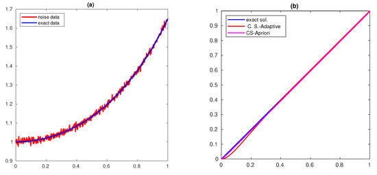
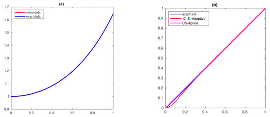
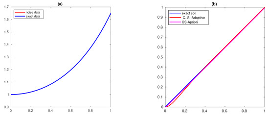
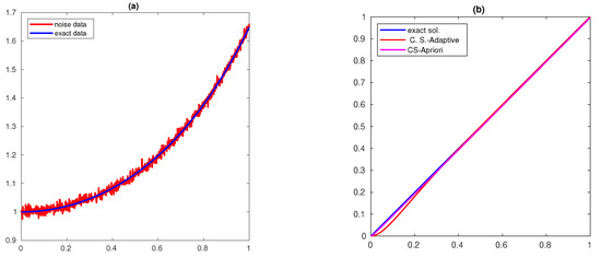
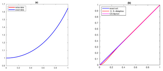
The solutions obtained for different δ values ($\delta =0.01,0.001,0.0001$) for $n=500$ are shown in Figure 1, Figure 2 and Figure 3, respectively, and for $n=1000$ and $\delta =0.01,0.001,0.0001$ are shown in Figure 4, Figure 5 and Figure 6, respectively. The exact and noisy data are shown in subfigure (a) of these figures and the computed solution is shown in subfigure(b) (C.S-A priori denotes the figure corresponding to the method (51)). The computed solution for the new method is closer to the actual solution.

Figure 1. (a) data and (b) Solution with $\delta =0.01$ and $n=500$.

Figure 2. (a) data and (b) Solution with $\delta =0.001$ and $n=500$.

Figure 3. (a) data and (b) Solution with $\delta =0.0001$ and $n=500$.

Figure 4. (a) data and (b) Solution with $\delta =0.01$ and $n=1000$.

Figure 5. (a) data and (b) Solution with $\delta =0.001$ and $n=1000$.

Figure 6. (a) data and (b) Solution with $\delta =0.0001$ and $n=1000$.

6. Conclusions

We introduced a new source condition and a new parameter-choice strategy. The proposed a new parameter-choice strategy is independent of the unknown parameter $\nu$ and it provides the optimal order $O\left({\delta }^{\frac{\nu }{\nu +1}}\right),$ for $0\le \nu \le 1.$

References

- George, S.; Nair, M.T. A modified Newton-Lavrentiev regularization for non-linear ill-posed Hammerstein-type operator equations. J. Complex. 2008, 24, 228–240. [Google Scholar] [CrossRef]
- Hofmann, B.; Kaltenbacher, B.; Resmerita, E. Lavrentiev’s regularization method in Hilbert spaces revisited. Inverse Probl. Imaging 2016, 10, 741–764. [Google Scholar] [CrossRef]
- Janno, J.; Tautenhahn, U. On Lavrentiev regularization for ill-posed problems in Hilbert scales’. Numer. Funct. Anal. Optim. 2003, 24, 531–555. [Google Scholar] [CrossRef]
- Mahale, P.; Nair, M.T. Lavrentiev regularization of non-linear ill-posed equations under general source condition. J. Nonlinear Anal. Optim. 2013, 4, 193–204. [Google Scholar]
- Tautenhahn, U. On the method of Lavrentiev regularization for non-linear ill-posed problems. Inverse Probl. 2002, 18, 191–207. [Google Scholar] [CrossRef]
- Vasin, V.; George, S. An analysis of Lavrentiev regularization method and Newton type process for non-linear ill-posed problems. Appl. Math. Comput. 2014, 230, 406–413. [Google Scholar]
- Nair, M.T.; Ravishankar, P. Regularized versions of continuous Newton’s method and continuous modified Newton’s method under general source conditions. Numer. Funct. Anal. Optim. 2008, 29, 1140–1165. [Google Scholar] [CrossRef]
- George, S.; Sreedeep, C.D. Lavrentiev’s regularization method for nonlinear ill-posed equations in Banach spaces. Acta Math. Sci. 2018, 38B, 303–314. [Google Scholar] [CrossRef]
- George, S. On convergence of regularized modified Newton’s method for non-linear ill-posed problems. J. Inverse Ill-Posed Probl. 2010, 18, 133–146. [Google Scholar] [CrossRef]
- Semenova, E.V. Lavrentiev regularization and balancing principle for solving ill-posed problems with monotone operators. Comput. Methods Appl. Math. 2010, 10, 444–454. [Google Scholar] [CrossRef]
- De Hoog, F.R. Review of Fredholm equations of the first kind. In The Application and Numerical Solution of Integral Equations; Anderssen, R.S., De Hoog, F.R., Luckas, M.A., Eds.; Sijthoff and Noordhoff: Alphen aan den Rijn, The Netherlands, 1980; pp. 119–134. [Google Scholar]
- Krasnoselskii, M.A.; Zabreiko, P.P.; Pustylnik, E.I.; Sobolevskii, P.E. Integral Operators in Spaces of Summable Functions; Noordhoff International Publishing: Leyden, The Netherlands, 1976. [Google Scholar]
- Mahale, P.; Nair, M.T. Iterated Lavrentiev regularization for non-linear ill-posed problems. ANZIAM J. 2009, 51, 191–217. [Google Scholar] [CrossRef]
- Argyros, I.K. The Theory and Applications of Iteration Methods, 2nd ed.; Engineering, Series; CRC Press: Boca Raton, FL, USA; Taylor and Francis Group: Abingdon, UK, 2022. [Google Scholar]
- Argyros, I.K. Unified Convergence Criteria for Iterative Banach Space Valued Methods with Applications. Mathematics 2021, 9, 1942. [Google Scholar] [CrossRef]
- George, S.; Nair, M.T. A derivative–free iterative method for nonlinear ill-posed equations with monotone operators. J. Inverse Ill-Posed Probl. 2017, 25, 543–551. [Google Scholar] [CrossRef]
- Kaltenbacher, B. Some Newton-type methods for the regularization of nonlinear ill-posed problems. Inverse Probl. 1997, 13, 729–753. [Google Scholar] [CrossRef]
- Deimling, K. Nonlinear Functional Analysis; Springer: New York, NY, USA, 1985. [Google Scholar]
- Alber, Y.; Ryazantseva, I. Nonlinear Ill-Posed Problems of Monotone Type; Springer: Berlin/Heidelberg, Germany, 2006. [Google Scholar]
- Nair, M.T. Functional Analysis: A First Course; Fourth Print, 2014; PHI-Learning: New Delhi, India, 2002. [Google Scholar]
- Groetsch, C.W.; King, J.T.; Murio, D. Asymptotic analysis of a finite element method for Fredholm integral equations of the first kind. In Treatment of Integral Equations by Numerical Methods; Baker, C.T.H., Miller, G.F., Eds.; Academic Press: Cambridge, MA, USA, 1982; pp. 1–11. [Google Scholar]
- Hofmann, B.; Scherzer, O. Factors influencing the ill-posedness of nonlinear inverse problems. Inverse Probl. 1994, 10, 1277–1297. [Google Scholar] [CrossRef]
- Groetsch, C.W. Inverse Problems in the Mathematical Sciences; Vieweg: Braunschweig, Germany, 1993. [Google Scholar]
- Pereverzev, S.; Schock, E. On the adaptive selection of the parameter in regularization of ill-posed problems. SIAM J. Numer. Anal. 2005, 43, 2060–2076. [Google Scholar] [CrossRef]
Publisher’s Note: MDPI stays neutral with regard to jurisdictional claims in published maps and institutional affiliations. |
© 2022 by the authors. Licensee MDPI, Basel, Switzerland. This article is an open access article distributed under the terms and conditions of the Creative Commons Attribution (CC BY) license (https://creativecommons.org/licenses/by/4.0/).