A Numerical Scheme for Harmonic Stochastic Oscillators Based on Asymptotic Expansions

Abstract

In this work, we provide a numerical method for discretizing linear stochastic oscillators with high constant frequencies driven by a nonlinear time-varying force and a random force. The presented method is constructed by starting from the variation of constants formula, in which highly oscillating integrals appear. To provide a suited discretisation of this type of integrals, we propose quadrature rules based on asymptotic expansions. Theoretical considerations and numerical experiments comparing the method with a standard approach on physical models are introduced.

1. Introduction

Scientific literature provides a wide variety of models of oscillators both in deterministic and in stochastic fields. Stochastic oscillators are often obtained by the introduction of a noisy component in a deterministic oscillatory model. The work in [1] includes a valuable survey on stochastic oscillators. In this paper, we are interested in a second-order differential problem of the following form:

$$\ddot{x}=-{\omega }^{2}x+g\left(t\right)+\epsilon \xi \left(t\right),$$

(1)

where $\xi \left(t\right)$ is a white noise process satisfying $\mathbb{E}|\xi \left(t\right)\xi \left(t^{\prime }\right)|=\delta (t-t^{\prime })$ and $\omega$ is a positive real constant. Stochastic harmonic undamped oscillators driven by both a deterministic time-dependent force and a random Gaussian forcing are modelled by equations as shown in Equation (1). This kind of stochastic oscillators is widespread in the physics literature (see [1,2,3,4,5]). We suppose $\omega$ is large (i.e., a high oscillating model). Since standard numerical integrators are not indicated in these cases, specific numerical treatments for approximating their solutions are required. In the numerical analysis literature, several works are concerned with analyzing different aspects of stochastic oscillators. The main numerical issues investigated in stochastic oscillating models are the construction of numerical methods adapted to a considered particular model, as in [6,7,8,9,10,11], and the attitude of numerical methods to preserve quantities in the long term, as investigated in [12,13,14,15,16,17,18,19,20]. We follow an idea similar to that in [8], in which the authors started from the variation of constants formula and, after suited discretisations of the involved integrals were found, provided a numerical strategy for the considered model. In this case, we involve a quadrature rule based on the asympotic expansions, (see [21,22,23]). In [24], the author introduced efficient numerical approximations for linear and nonlinear systems of highly oscillatory ordinary differential equations and showed how an appropriate choice of quadrature rule improves the accuracy of the approximation as the frequency of oscillation grows. We try to extend such an idea in the presence of additive Gaussian noise. The employment of the variation of constants formula to design numerical schemes suited for oscillatory problems is widespread in the deterministic setting (see [25,26] and the references therein). It has also recently become a starting point in the construction of methods in stochastic equations. In this regard, it can be mentioned the methods derived in [6,7] for nonlinear stochastic equations of the form

$$\ddot{x}=-{\omega }^{2}x+f\left(x\right)+\epsilon \xi \left(t\right)$$

are the stochastic counterpart of the deterministic trigonometric methods. A trigonometrically fitted approach for other types of equations may be found in [27,28]. This paper is organised as follows. In Section 2.2, we propose a semi-discretisation of the model based on a variation constants formula. In Section 2.3, we recall the main aspects of quadrature formulas based on asymptotic expansion and present the employed numerical method. In Section 3.1, numerical simulations are provided.

2. Construction of the Method

2.1. Recalls and Preparatory Notions

Let us remember that, given the stochastic differential equation

$$dX\left(t\right)=f\left(X\right(t\left)\right)dt+g\left(X\right(t\left)\right)dW\left(t\right),t\ge 0,$$

(2)

$f:{\mathbb{R}}^d\to {\mathbb{R}}^d$, $g:{\mathbb{R}}^d\to {\mathbb{R}}^{d\times m}$, and $W\left(t\right)$ is the m-dimensional Wiener process. Therefore, we can consider the integral form of Equation (2), given by

$$X\left(t\right)=X\left(0\right)+{\int }_0^{t}f\left(X\left(s\right)\right)\mathrm{d}s+{\int }_0^{t}g\left(X\left(s\right)\right)\mathrm{d}W\left(s\right).$$

On a uniform grid $\mathcal{I}=\{0\equiv t_0<t_1<t_2<\cdots <t_n\equiv t\}$, the stochastic integral is defined as an Ito integral if

$${\int }_0^{t}g\left(X\left(s\right)\right)\mathrm{d}W\left(s\right)=\underset{n\to \infty }{lim}\sum _{j=0}^{n-1}g\left(X\left(t_j\right)\right)\Delta W_j,$$

such that $\Delta W_j=W\left(t_{j+1}\right)-W\left(t_j\right)\approx \sqrt{h}·\mathcal{N}(0,1),$ where $h=t_{j+1}-t_j$. In this case, Equation (2) is said to be an Ito stochastic differential equation.

We recall now the Euler–Maruyama method, which is a standard approach for providing a numerical discretisation of a stochastic differential equation. Given a partition of the interval $[0,T]$ into N equal subintervals of a width h such that

$$0=t_0<t_1<...<t_n=T$$

and an initial condition $X\left(0\right)=X_0$, the explicit Euler–Maruyama method applied to Equation (2) is recursively defined as

$$X^{n+1}=X^n+hf\left(X^n\right)+g\left(X^n\right)\Delta W_n$$

where $X^n\approx X\left(t_n\right)$ and $\Delta W_n=W\left(t_{n+1}\right)-W\left(t_n\right)$. We refer to [29,30] for an extensive discussion on basic concepts of numerical analysis for stochastic differential equations and to [31,32,33,34] for recent results on standard numerical techniques for SDEs. Since the method is explicit, Euler–Maruyama suffers a lot from step size reduction when it is applied to a stiff problem, such as Equation (1) with $\omega \gg 1$. The main idea is to construct a numerical method based on the variation of constants formula, combined with a suited quadrature rule to provide full discretisation. We are motivated by the fact that the use of the variation of constants formula to derive an efficient numerical method for stiff problems is not new, as it has been extensively and successfully employed in deterministic cases (see [26] and the references therein) and also recently in the stochastic setting (see [7,8,9]). The application of the variation of constants formula will provide highly oscillatory integrals that we aim to discretise via the asymptotic quadrature method, which is specialised for this type of integral. This will overcome the problems related to the standard approach.

2.2. Semidiscretisation Based on Variation of Constants

Equation (1) is equivalent to the following first-order system of two Ito equations in the variables $X_t$ (the position of the particle) and $V_t$ (its velocity):

$$\left\{\begin{array}{c}d{X}_t=V_{t}dt\hfill \\ d{V}_t=-{\omega }^2{X}_{t}dt+g\left(t\right)dt+\epsilon d{W}_t,\hfill \end{array}\right.$$

(3)

Let us consider the matrix

$$A_{\omega }=\left[\begin{array}{cc}0& 1\\ -{\omega }^2& 0\end{array}\right],$$

whose expontential is given by

$$e^{t{A}_{\omega }}=\left[\begin{array}{cc}cos\left(t\omega \right)& {\omega }^{-1}sin\left(t\omega \right)\\ -\omega sin\left(t\omega \right)& cos\left(t\omega \right)\end{array}\right].$$

The variation of constants formula applied to the system in Equation (3) is given by

$$\begin{array}{cc}\hfill \left(\begin{array}{c}{X}_t\\ V_t\end{array}\right)=& e^{t{A}_{\omega }}\left(\begin{array}{c}{X}_0\\ V_0\end{array}\right)+{\int }_0^t\left(\begin{array}{c}{\omega }^{-1}sin\left((t-s)\omega \right)\\ cos\left(\right(t-s\left)\omega \right)\end{array}\right)g\left(s\right)ds\hfill \\ \hfill & +\epsilon {\int }_0^t\left(\begin{array}{c}{\omega }^{-1}sin\left((t-s)\omega \right)\\ cos\left(\right(t-s\left)\omega \right)\end{array}\right)d{W}_s,\hfill \end{array}$$

(4)

Referring to the uniform grid $\mathcal{I}$, after a standard discretisation in the stochastic part, we obtain

$$\begin{array}{cc}\hfill \left(\begin{array}{c}{X}_{n+1}\\ V_{n+1}\end{array}\right)=& e^{h{A}_{\omega }}\left(\begin{array}{c}{X}_n\\ V_n\end{array}\right)+{\int }_{t_n}^{t_{n+1}}\left(\begin{array}{c}{\omega }^{-1}sin\left((t_{n+1}-s)\omega \right)\\ cos\left((t_{n+1}-s)\omega \right)\end{array}\right)g\left(s\right)ds\hfill \\ \hfill & +\epsilon \left(\begin{array}{c}{\omega }^{-1}sin\left(h\omega \right)\\ cos\left(h\omega \right)\end{array}\right)\Delta W_n,\hfill \end{array}$$

(5)

where $\Delta W_n=W\left(t_{n+1}\right)-W\left(t_n\right)$ denotes the Wiener increment. In order to find a full discretisation, we must indicate how to proceed with the integral involving the deterministic force $g\left(t\right)$.

2.3. Numerical Method Based on Asymptotic Expansions

In this section, we recall some relevant issues of the asymptotic expansion quadrature for vector-valued integrals, following the approach of [24,35,36]. Let us introduce the vector-valued integral over the compact interval $[a,b]$:

$$I\left(\mathbf{f}\right)={\int }_a^b{X}_{\omega }\left(t\right)\mathbf{f}\left(t\right)dt,X_{\omega }^{\prime }=A_{\omega }{X}_{\omega },$$

(6)

where the matrix $X_{\omega }$ satisfies a linear differential equation (Equation (6)) with a constant non-singular matrix $A_{\omega }$ of large eigenvalues, $\left|\right|A_{\omega }{\left|\right|}_F\ll 1$, $\sigma \left(A_{\omega }\right)\subset ı\mathbb{R}$, $\omega$ is a real parameter, and $\mathbf{f}\in {\mathbb{R}}^n$ is a smooth vector-valued function. Since $X_{\omega }$ is the solution of the linear matrix differential equation in Equation (6), we can integrate Equation (6) in parts as follows:

$$I\left(\mathbf{f}\right)=A_{\omega }^{-1}[X_{\omega }\left(b\right)\mathbf{f}\left(b\right)-X_{\omega }\left(a\right)\mathbf{f}\left(a\right)]-A_{\omega }^{-1}{\int }_a^b{X}_{\omega }\left(t\right){\mathbf{f}}^{\prime }\left(t\right)dt=Q_1^A-A_{\omega }^{-1}I\left({\mathbf{f}}^{\prime }\right),$$

The asymptotic method is given by the s-partial sum of the asymptotic expansion for $I\left(\mathbf{f}\right)$, expressed as

$$Q_s^A=-\sum _{m=1}^s{A}_{\omega }^{-m}[X_{\omega }\left(b\right){\mathbf{f}}^{(m-1)}\left(b\right)-X_{\omega }\left(a\right){\mathbf{f}}^{(m-1)}\left(a\right)],$$

Proposition 1

([24]). If $X_{\omega }=\mathcal{O}\left(\mathbf{1}\right)$ and $\mathbf{f}=\mathcal{O}\left(\mathbf{1}\right)$, then

$$Q_s^A-I\left(\mathbf{f}\right)=\mathcal{O}\left(A_{\omega }^{-s-1}\mathbf{I}\right),$$

for $\omega ⟶\infty$.

The numerical strategy based on Equation (5) is defined by computing

$$I_h\left(\mathbf{f}\right)={\int }_0^h{e}^{A_{\omega }(h-t)}\mathbf{f}(t_n+t)dt,$$

where $\mathbf{f}\left(t\right)={\left[0g\left(t\right)\right]}^{\prime }$. By the asymptotic method for $s=2$, we have

$$Q_A^2=-A_{\omega }^{-1}(\mathbf{f}\left(t_{n+1}\right)-e^{A_{\omega }h}\mathbf{f}\left(t_n\right))-A_{\omega }^{-2}({\mathbf{f}}^{\prime }\left(t_{n+1}\right)-e^{A_{\omega }h}{\mathbf{f}}^{\prime }\left(t_n\right)),$$

3. Numerical Experiments

In this section, we provide a numerical study of the properties of convergence of the presented method. In particular, we show what we essentially expect (i.e., that as the frequency $\omega$ grows, the numerical estimated order of convergence improves significantly, and the method definitively outperforms a standard approach such as Euler–Maruyama in terms of accuracy and computational times). In particular, for the accuracy, we show the behaviour of the mean square errors with respect to the step size h, computed considering $M={10}^4$ paths. To compare the methods with respect to the computational times, we evaluated the time taken for each method to perform $M=100$ paths. The results are shown in Table 1. Each time reported is the average of 15 experiments conducted on the examples discussed below.

Table 1. Table of the computational times on the three examples, considering $M=100$ paths and comparing the asymptotic and Euler–Maruyama methods.

Method	Example 1	Example 2	Example 3
Asymptotic Method	$24.12$ s	$41.5$ s	$23.4$ s
Euler–Maruyama	$27.63$ s	$43.08$ s	$28.8$ s

3.1. Example 1

We propose a very popular example in the physics literature (see [1,3,37]):

$$\left\{\begin{array}{c}d{X}_t=V_{t}dt\hfill \\ d{V}_t=-{\omega }^2{X}_{t}dt-Qcos\left(\mathsf{\Omega }t\right)dt+\epsilon d{W}_t\hfill \end{array}\right.$$

(7)

We integrated Equation (7) over the interval $[0,1]$ with the initial conditions $X_0=1$ and $V_0=1$. In [24], we could find a similar example, so we can consider Equation (7) as a stochastic perturbation. The values of the constants were $Q=10$, $\mathsf{\Omega }=5$, and $\epsilon =0.3$. In Figure 1, we plotted the mean square error in the position with respect to the step size for different values of $\omega$. In Figure 2, we did the same for the error in the velocity. We can observe that the method had an accuracy increasing with ${\omega }^2$, which is typical in the deterministic setting when the asymptotic expansion is used. In Figure 3, we show the comparison between the Euler–Maruyama method and the method discussed in this work in terms of the mean square errors in the position for ${\omega }^2={10}^4$. It appears clear that the Euler–Maruyama method is not suited for the considered high-oscillation problems.

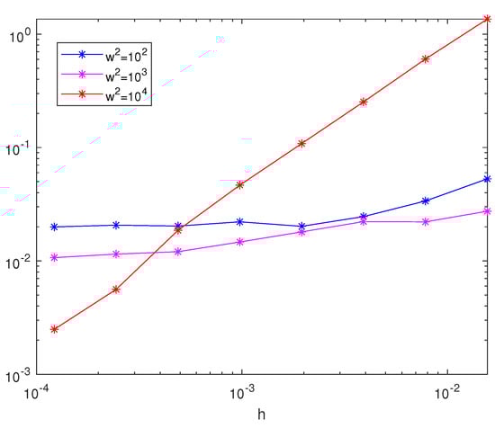
Figure 1. A figure showing the mean square errors in the position of the numerical solutions for Equation (7) for different values of ${\omega }^2$.

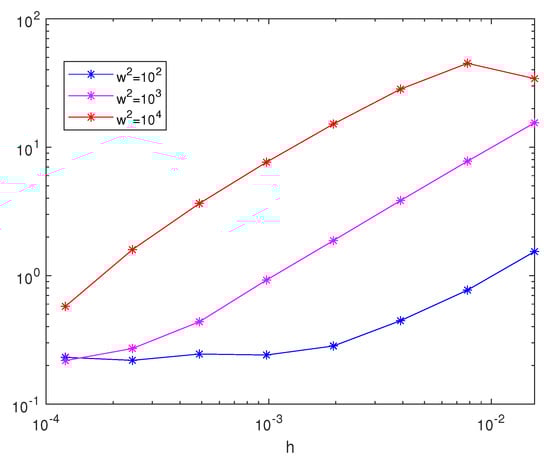
Figure 2. A figure showing the mean square errors in the velocity of the numerical solutions for Equation (7) for different values of ${\omega }^2$.

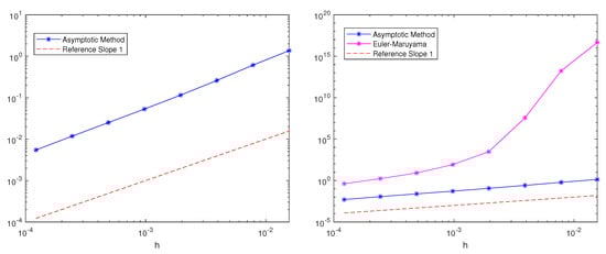
Figure 3. A figure showing the mean square errors in the position of the numerical solutions for Equation (7) for ${\omega }^2={10}^4$ for the asymptotic and Euler–Maruyama methods.

3.2. Example 2

Motivated by [23], we propose the following particular system:

$$\left\{\begin{array}{c}d{X}_t=V_{t}dt\hfill \\ d{V}_t=-{\omega }^2{X}_{t}dt+e^{i\sigma f\left(t\right)}dt+\epsilon d{W}_t\hfill \end{array}\right.$$

(8)

where $\epsilon =0.3$. We test the introduced method while considering $f\left(t\right)\equiv 1$ and then $f\left(t\right)=-t^2+t$. In Figure 4 (for $f\left(t\right)=-t^2+t$) and in Figure 5 (for $f\left(t\right)\equiv 1$), we show the plots of the mean square errors in the position for different values of $\omega$, and as before, we can conclude that the accuracy increased with $\omega$. In Figure 6 (for $f\left(t\right)=-t^2+t$) and Figure 7 (for $f\left(t\right)\equiv 1$), we show the comparison between the Euler–Maruyama method and the method discussed in this work in terms of the mean square errors in the position for ${\omega }^2={10}^4$.

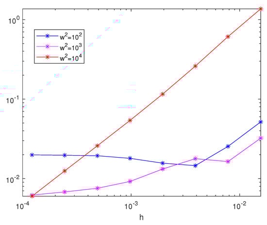
Figure 4. A figure showing the mean square errors in the position of the numerical solutions for Equation (Figure 4) with $f\left(t\right)=-t^2+t$ and $\sigma =10$ for different values of ${\omega }^2$.

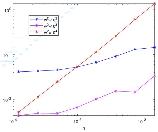
Figure 5. A figure showing the mean square errors in the position of the numerical solutions for Equation (Figure 4) with $f\left(t\right)\equiv 1$ and $\sigma =100$ for different values of ${\omega }^2$.

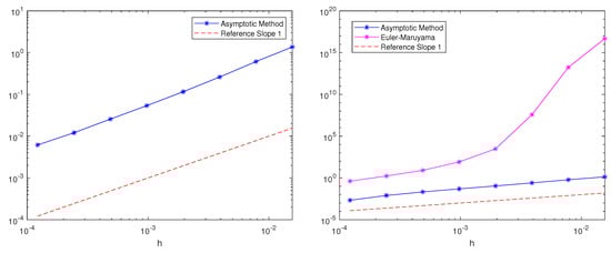
Figure 6. A figure showing the mean square errors in the position of the numerical solutions for Equation (8) for ${\omega }^2={10}^4$ for the asymptotic and Euler–Maruyama methods.

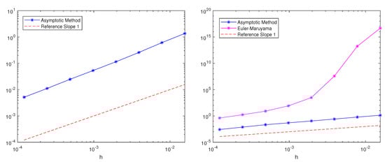
Figure 7. A figure showing the mean square errors in the position of the numerical solutions for Equation (7) for ${\omega }^2={10}^4$ for the asymptotic and Euler–Maruyama methods.

3.3. Example 3

The final example is described by the following system:

$$\left\{\begin{array}{c}d{X}_t=V_{t}dt\hfill \\ d{V}_t=-{\omega }^2{X}_{t}dt-Q{cos}^2\left(\mathsf{\Omega }t\right)dt-Psin\left(\mathsf{\Lambda }t\right)\epsilon d{W}_t\hfill \end{array}\right.$$

(9)

We fixed the parameters such that $Q=10$, $P=20$, $\mathsf{\Omega }=5$, and $\mathsf{\Lambda }=7$. The time-dependent force was a nonlinear combination of trigonometric functions, which is typical for these problems (see [1]). In addition, in this case, we confirmed that the asymptotic-based method had better performance (see Figure 8).

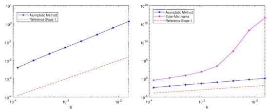
Figure 8. A figure showing the mean square errors in the position of the numerical solutions for Equation (9) for ${\omega }^2={10}^4$ for the asymptotic and Euler–Maruyama methods. On the right are the behaviours of both methods. On the left are the behaviour of the asymptotic method.

4. Conclusions

In this paper, we combined two typical ingredients of the numerics for ODEs (i.e., variation of constants (related to trigonometric methods) and asymptotic expansion quadrature) to define a full numerical strategy for second-order stochastic equations of the type in Equation (1). Numerical experiments on models of oscillators, which are widespread in the literature, showed their behaviour and confirmed the correctness of the approach. We can see in all the experiments that for a growing $\omega$, the mean square order of accuracy improved up to one. In particular, the method is suited for problems in which $\omega$ becomes very large, thanks to the use of the asymptotic quadrature for highly oscillating integrals. In this case, as we can expect, standard approaches for solving stochastic differential equations, such as the Euler–Maruyama method, are able to correctly simulate the solution only for choices of the step size which are very small. Numerical experiments showed that the asymptotic quadrature-based approach proposed in the presented paper outperformed the standard approach. On the other hand, when the frequency does not assume particularly large values, more traditional numerical methods for SDEs may be sufficient to discretise the system. Future perspectives in this field may involve a rigorous proof of convergence and possible extension of the method to stochastic oscillators with multiplicative noise.

References

- Gitterman, M. The Noisy Oscillator. The First Hundred Years, from Einstein Until Now; World Scientific Publishing Company: Singapore, 2005. [Google Scholar]
- Giorgini, A.; Mamon, R.S.; Rodrigo, M.R. A stochastic harmonic oscillator temperature model for the valuation of weather derivatives. Mathematics 2021, 9, 2890. [Google Scholar] [CrossRef]
- Gitterman, M. Oscillator Subject to Periodic and Random Forces. J. Mod. Phys. 2013, 4, 94–98. [Google Scholar] [CrossRef][Green Version]
- Lingala, N.; Namachchivaya, N.; Pavlyukevich, I. Random perturbations of a periodically driven nonlinear oscillator: Escape from a resonance zon. Nonlinearity 2017, 30, 1376–1404. [Google Scholar] [CrossRef]
- Thomas, P.J.; Linder, B. Asymptotic phase for stochastic oscillators. Phys. Rev. Lett. 2014, 113, 254101. [Google Scholar] [CrossRef] [PubMed]
- Cohen, D. On the numerical discretisation of stochastic oscillators. Math. Comput. Simul. 2012, 82, 1478–1495. [Google Scholar] [CrossRef]
- Cohen, D.; Sigg, M. Convergence analysis of trigonometric methods for stiff second-order stochastic differential equations. Numer. Math. 2012, 121, 1–29. [Google Scholar] [CrossRef][Green Version]
- D’Ambrosio, R.; Scalone, C. Filon quadrature for stochastic oscillators driven by time-varying forces. Appl. Numer. Math. 2021, 169, 21–31. [Google Scholar] [CrossRef]
- D’Ambrosio, R.; Scalone, C. Asymptotic Quadrature Based Numerical Integration of Stochastic Damped Oscillators. In International Conference on Computational Science and Its Applications; Lecture Notes in Computer Science (including subseries Lecture Notes in Artificial Intelligence and Lecture Notes in Bioinformatics); Springer: Cham, Switzerland, 2021; Volume 12950, pp. 622–629. [Google Scholar]
- de la Cruz, H.; Jimenez, J.C.; Zubelli, J.P. Locally linearized methods for the simulation of stochastic oscillators driven by random forces. BIT Numer. Math. 2017, 57, 123–151. [Google Scholar] [CrossRef]
- Senoisian, M.J.; Tocino, A. On the numerical integration of the undamped harmonic oscillator driven by independent additive gaussian white noises. Appl. Numer. Math. 2019, 137, 49–61. [Google Scholar] [CrossRef]
- Burrage, K.; Lenane, I.; Lythe, G. Numerical methods for second-order stochastic differential equations. SIAM J. Sci. Comput. 2007, 29, 245–264. [Google Scholar] [CrossRef]
- Burrage, K.; Lythe, G. Accurate stationary densities with partitioned numerical methods for stochastic differential equations. SIAM J. Numer. Anal. 2009, 47, 1601–1618. [Google Scholar] [CrossRef]
- Citro, V.; D’Ambrosio, R. Long-term analysis of stochastic θ-methods for damped stochastic oscillators. Appl. Numer. Math. 2019, 150, 18–26. [Google Scholar] [CrossRef]
- D’Ambrosio, R.; Giovacchino, S.D.; Scalone, C. Principles of Stochastic Geometric Numerical Integrations: Dissipative Problems and Stochastic Oscillators. In AIP Conference Proocedings of ICNAAM; American Institute of Physics: College Park, MD, USA, 2021. [Google Scholar]
- D’Ambrosio, R.; Moccaldi, M.; Paternoster, B. Numerical preservation of long-term dynamics by stochastic two-step methods. Discret. Contin. Dyn. Syst. Ser. B 2018, 23, 2763–2773. [Google Scholar] [CrossRef]
- D’Ambrosio, R.; Scalone, C. On the numerical structure preservation of nonlinear damped stochastic oscillators. Numer. Algorithms 2021, 86, 933–952. [Google Scholar] [CrossRef]
- Scalone, C. Positivity preserving stochastic θ-methods for selected SDEs. Appl. Numer. Math. 2022, 172, 351–358. [Google Scholar] [CrossRef]
- Strömmen Melbö, A.H.; Higham, D.J. Numerical simulation of a linear stochastic oscillator with additive noise. Appl. Numer. Math. 2004, 51, 89–99. [Google Scholar] [CrossRef]
- Tocino, A. On preserving long-time features of a linear stochastic oscillator. BIT Numer. Math. 2007, 47, 189–196. [Google Scholar] [CrossRef]
- Iserles, A.; Nørsett, S.P. On Quadrature Methods for Highly Oscillatory Integrals and Their Implementation. BIT Numer. Math. 2004, 44, 755–772. [Google Scholar] [CrossRef]
- Iserles, A.; Nørsett, S.P. Efficient quadrature of highly oscillatory integrals using derivatives. Proc. R. Soc. A 2006, 461, 1383–1399. [Google Scholar] [CrossRef]
- Condon, M.; Iserles, A.; Nørsett, S.P. Differential equations with general highly oscillatory forcing terms. Proc. R. Soc. A 2014, 470. [Google Scholar] [CrossRef]
- Khanamiryan, M. Quadrature methods for highly oscillatory linear and nonlinear systems of ordinary differential equations: Part I. BIT Numer. Math. 2008, 48, 743. [Google Scholar] [CrossRef]
- Hairer, E.; Lubich, C.; Wanner, G. Geometric Numerical Integration; Springer: Berlin/Heidelberg, Germany, 2006. [Google Scholar]
- Hochbruck, M.; Ostermann, A. Exponential Integrators. Acta Numer. 2010, 19, 209–286. [Google Scholar] [CrossRef]
- Shokri, A. An explicit trigonometrically fitted ten-step method with phase-log of order infinity for the numerical solution of the radiale Schrodinger equation. Appl. Comput. Math. 2015, 14, 63–74. [Google Scholar]
- Shokri, A.; Saadat, H.; Khodadadi, A.R. A New High Order Closed Newton-Cotes Trigonometrically-fitted Formulae for the Numerical Solution of the Schrodinger Equation. Iran. J. Math. Sci. Inform. 2018, 13, 111–129. [Google Scholar]
- Kloeden, P.E.; Platen, E. The Numerical Solution of Stochastic Differential Equations; Springer: Berlin/Heidelberg, Germany, 1992. [Google Scholar]
- Mao, X. Stochastic Differential Equations and Applications, 2nd ed.; Woodhead Publishing: Cambridge, UK, 2008. [Google Scholar]
- D’Ambrosio, R.; Guglielmi, N.; Scalone, C. Destabilising nonnormal stochastic differential equations. Dicrete Contin. Dyn. Syst. Ser. B 2022. [Google Scholar] [CrossRef]
- D’Ambrosio, R.; Giovacchino, S.D. Numerical preservation issues in stochastic dynamical systems by θ-methods. J. Comput. Dyn. 2022, 9, 123–131. [Google Scholar] [CrossRef]
- D’Ambrosio, R.; Giovacchino, S.D. Mean-square contractivity of stochastic θ-methods. Commun. Nonlinear Sci. Numer. Simul. 2021, 96, 105671. [Google Scholar] [CrossRef]
- Ruan, J.; Wang, L.; Wang, P. Exponential discrete gradient schemes for a class of stochastic differential equations. J. Comput. Appl. Math. 2022, 402, 113–797. [Google Scholar] [CrossRef]
- Khanamiryan, M. Quadrature methods for highly oscillatory linear and non-linear systems of ordinary differential equations: Part II. BIT Numer. Math. 2012, 52, 383–405. [Google Scholar] [CrossRef]
- Olver, S. Numerical approximation of vector-valued highly oscillatory integrals. BIT Numer. Math. 2007, 47, 637–655. [Google Scholar] [CrossRef]
- Bulsara, A.R.; Lindenberg, K.; Shuler, K.E. Spectral analysis of a nonlinear oscillator driven by random and periodic forces. I. Linearized Theory. J. Stat. Phys. 1982, 27, 787–808. [Google Scholar] [CrossRef]
Publisher’s Note: MDPI stays neutral with regard to jurisdictional claims in published maps and institutional affiliations. |
© 2022 by the author. Licensee MDPI, Basel, Switzerland. This article is an open access article distributed under the terms and conditions of the Creative Commons Attribution (CC BY) license (https://creativecommons.org/licenses/by/4.0/).