Comparative Analysis of Different Iterative Methods for Solving Current–Voltage Characteristics of Double and Triple Diode Models of Solar Cells

Abstract

The current–voltage characteristics of the double diode and triple diode models of solar cells are highly nonlinear functions, for which there is no analytical solution. Hence, an iterative approach for calculating the current as a function of voltage is required to estimate the parameters of these models, regardless of the approach (metaheuristic, hybrid, etc.) used. In this regard, this paper investigates the performance of four standard iterative methods (Newton, modified Newton, Secant, and Regula Falsi) and one advanced iterative method based on the Lambert W function. The comparison was performed in terms of the required number of iterations for calculating the current as a function of voltage with reasonable accuracy. Impact of the initial conditions on these methods’ performance and the time consumed was also investigated. Tests were performed for different parameters of the well-known RTC France solar cell and Photowatt-PWP module used in many research works for the triple and double diode models. The advanced iterative method based on the Lambert W function is almost independent of the initial conditions and more efficient and precise than the other iterative methods investigated in this work.

1. Introduction

Since the first energy crisis in October 1973, much attention has been paid to renewable energy research [1,2]. The penetration of renewable energies into modern energy systems reduces the harmful effects of fossil fuel use, reduces power losses in transmission and distribution networks, improves voltage conditions, and expands the independent energy resources for consumers [3]. Renewables, particularly solar and wind energies [4], and energy storage systems are the basis for the development of modern energy systems [5]. At present, the critical indicator affecting energy security in any country is the stable operation of the energy system. Unfortunately, climate change, political crises, epidemics, and wars significantly impact the energy transition to carbon-free energy systems [6]. As a result, most countries have strengthened their renewable plans to reduce fossil fuel use and achieve green energy independence [7,8].

In this context, the solar cell is an energy component in which the sun’s energy is transformed into electricity. Solar cells are connected in series and parallel into solar arrays and modules, forming solar panels. In mathematical terms, a solar cell/module/array or panel is described by a nonlinear current and voltage relationship [9]. The simplest solar cell model is the single diode model (SDM) [10]. It is a model that comprises one current generator, a source of photocurrent, two resistors (series and parallel) representing losses in the solar cell, and one diode. As the diode is described with two unknown parameters (saturation current and ideal factor), the SDM is called the five-parameter model [11,12,13]. The classic five-parameter model is the most widely accepted but also the least accurate model of solar cells. Improved variants of this model can be found in [13], which include the existence of another resistor connected in series with the diode. However, it is essential to emphasize an analytical relationship between the current and voltage of this model, represented by the Lambert W function. A comparison of different methods for estimating the parameters of the SDM of solar cells and ways of solving the Lambert W function are presented in [11].

In addition to the SDM, there are double and triple diode models, DDM and TDM, of solar cells described in the available literature [14,15,16,17,18,19,20,21,22,23,24,25,26,27,28,29,30,31,32,33,34,35,36,37,38,39]. Moreover, modified versions of these models that include additional resistances and capacitances were also found [15]. In general, in the mathematical sense, the classical DDM and TDM of solar cells can be represented by a nonlinear function, for which there is no analytical solution. Therefore, for a specific current value, it is necessary to use iterative methods to calculate the voltage value or vice versa.

The application of iterative methods is necessary for estimating the parameters of DDM and TDM models of solar cells, regardless of the approach employed to estimate the parameters (metaheuristic algorithms, hybrid algorithms, combined analytical–iterative methods, or similar) [12,13,14,15,16,17,18,19,20,21,22,23,24,25,26,27,28,29,30,31,32,33,34,35,36,37,38,39]. In scientific publications, the dominant approach in estimating solar cell parameters is that the estimation is performed by minimizing the root-mean-square-error between the measured and estimated output solar current value [11,12,13]. However, very often, how the current is calculated as a function of voltage is not emphasized in these models.

This paper deals with the comparison of different iterative methods for the calculation of current as a function of voltage in DDMs and TDMs. To that goal, this work tests and compares four standard iterative methods—the Newton method (NM), modified Newton method (MNM), Secant method (SM), and Regula Falsi method (RFM), and one advanced iterative approach based on Lambert W function (LWF) proposed by the authors in [11,12,13] for SDMs and [14] for DDM and TDM. Some newly reported multiple root solvers with no derivatives can be found in the literature [40,41,42,43]. Therefore, the main contributions of this paper are outlined as follows:

• The paper points out the nonlinearity of the relationship between current and voltage in DDMs and TDMs;
• The paper compares different iterative methods for the calculation of current as a function of voltage for DMMs and TDMs;
• Based on the obtained results, the applicability of the tested methods is discussed;
• The time consumed by each of the mentioned methods is also analyzed;
• Special attention is paid to the impact of the initial conditions on the required number of iterations for a certain accuracy.

The rest of the paper is organized as follows. The Section 2 describes DDM and TDM and points out the nonlinearity of the current–voltage relations. In the Section 3, four well-known iterative methods for solving nonlinear equations are discussed, and one advanced iterative method based on the Lambert W function is introduced. The Section 4 compares the performance of the different iterative methods for calculating the current as a function of voltage using parameters, with sufficient details, for three well-known solar cells. A conclusion is included at the end of the paper, in which we point out the benefits and findings of the work and the potential directions for future research.

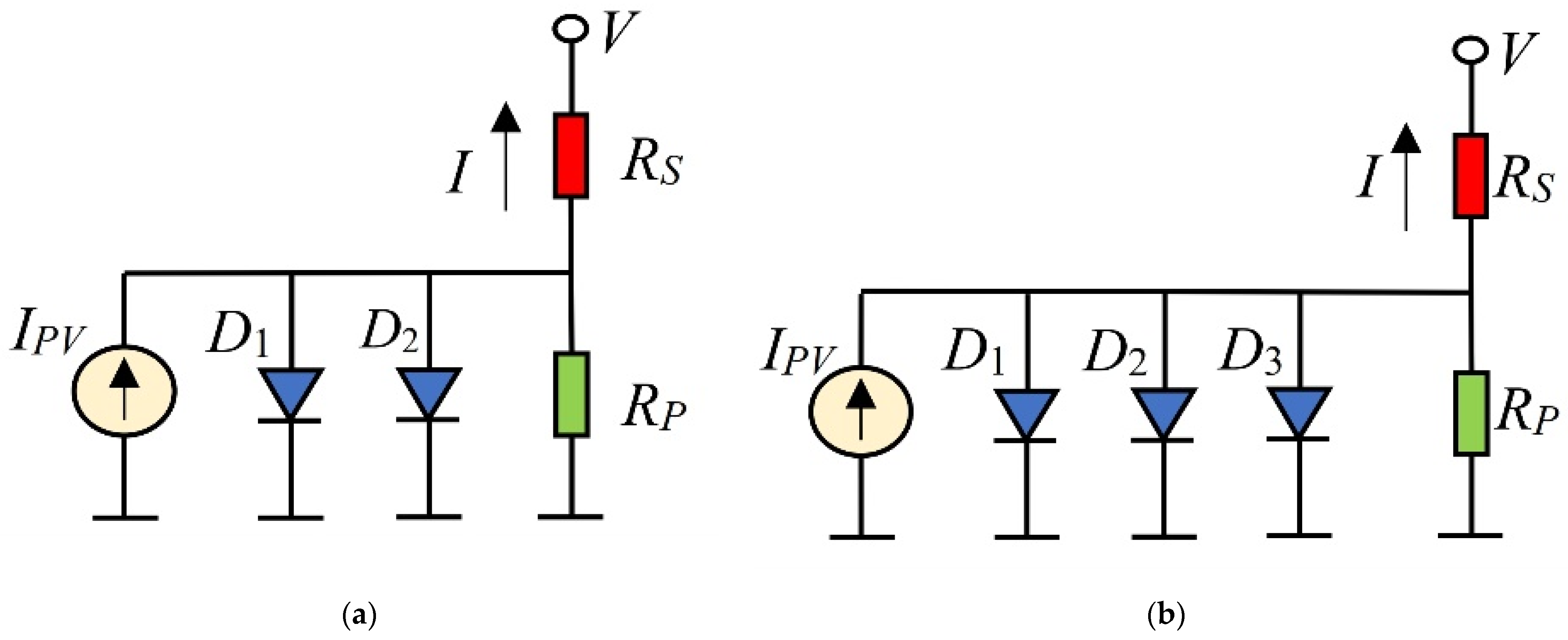
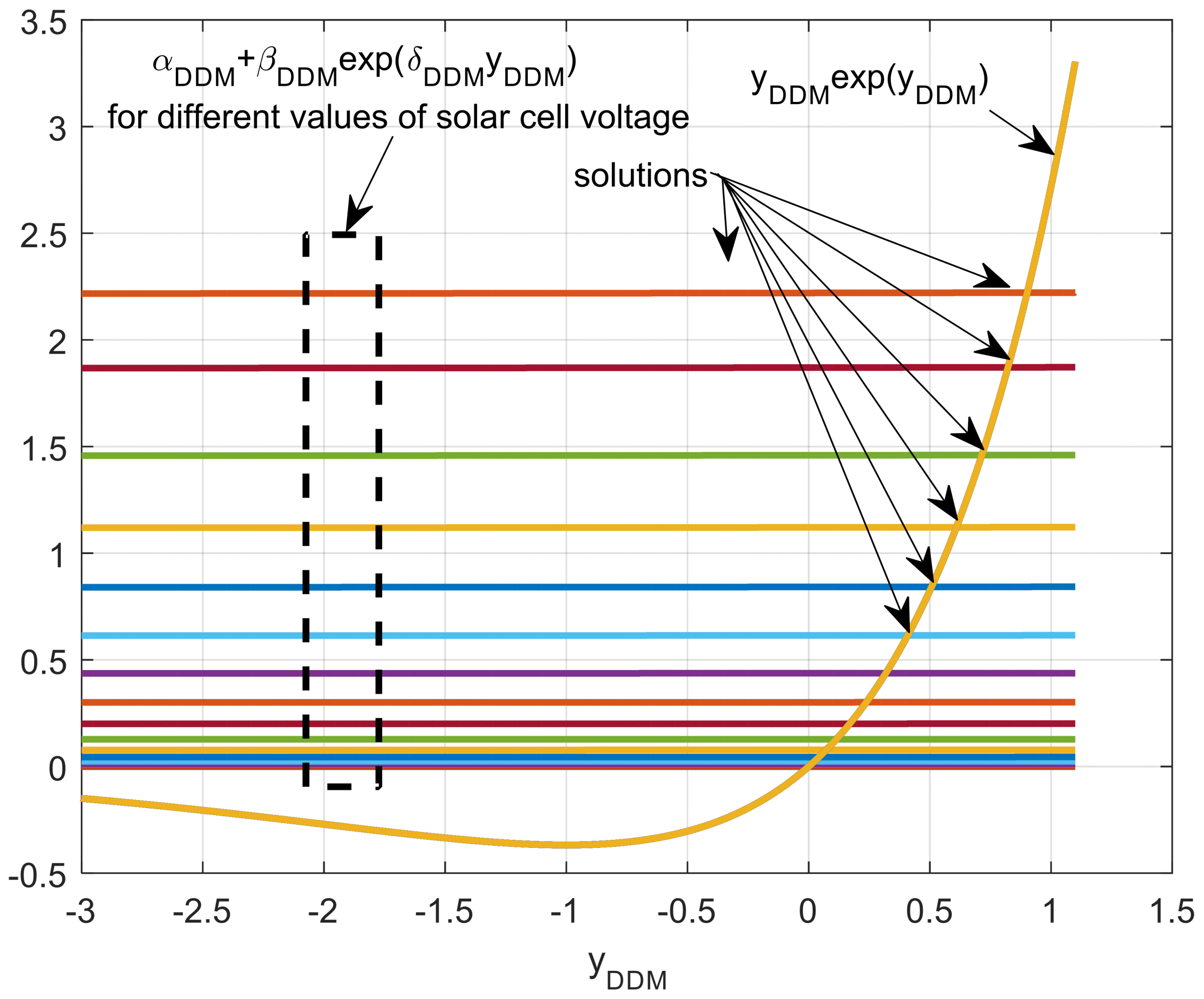
2. Double and Triple Diode Models

The standard equivalent circuits of the DDM and TDM are depicted in Figure 1. These circuits can be described using the following expressions, respectively:

$$I=I_{PV}-I_{01}\left(e^{\frac{V+I{R}_S}{n_1{V}_{th}}}-1\right)-I_{02}\left(e^{\frac{V+I{R}_S}{n_2{V}_{th}}}-1\right)-\frac{V+I{R}_S}{R_P},$$

(1)

$$I=I_{PV}-I_{01}\left(e^{\frac{V+I{R}_S}{n_1{V}_{th}}}-1\right)-I_{02}\left(e^{\frac{V+I{R}_S}{n_2{V}_{th}}}-1\right)-I_{03}\left(e^{\frac{V+I{R}_S}{n_3{V}_{th}}}-1\right)-\frac{V+I{R}_S}{R_P}.$$

(2)

where I_PV denotes the photo-generated current, I₀₁, I₀₂, and I₀₃ denote the reverse saturation current of the three diodes, respectively, n₁, n₂, and n₃ denote the ideality factors of the three diodes, and V_th = K_BT/q is the thermal voltage, where K_B denotes the Boltzmann constant in (JK⁻¹), T denotes the temperature in Kelvin and q denotes the charge of the electron in (C). It can be seen that both Equations (1) and (2) are highly nonlinear. For example, for the DDM equation, it can be seen that the current appears on the left side of the equation, in the first exponential part, which describes diode D₁, in the second exponential part, which describes diode D_2, and finally in the last part (on the right), which represents the current flowing through parallel resistance. Therefore, for DDM, the current appears in four places in the corresponding equation.

Equation (1) can be reformulated in the following manner [14]:

$${\alpha }_{DDM}+{\beta }_{DDM}{e}^{{\delta }_{DDM}{y}_{DDM}}=y_{DDM}{e}^{y_{DDM}},$$

(3)

where

$${\alpha }_{DDM}=\frac{R_S{R}_P}{R_S+R_P}\frac{I_{01}}{n_1{V}_{th}}{\mathrm{e}}^{\frac{V}{n_1{V}_{th}}}{\mathrm{e}}^{\frac{R_S{R}_P}{R_S+R_P}\frac{I_{PV}+I_{01}+I_{02}-\frac{V}{R_P}}{n_1{V}_{th}}},$$

(4)

$${\beta }_{DDM}=\frac{R_S{R}_P}{R_S+R_P}\frac{I_{02}}{n_1{V}_{th}}{\mathrm{e}}^{\frac{V}{n_2{V}_{th}}}{\mathrm{e}}^{\frac{R_S{R}_P}{R_S+R_P}\frac{I_{PV}+I_{01}+I_{02}-\frac{V}{R_P}}{n_2{V}_{th}}},$$

(5)

$${\delta }_{DDM}=1-\frac{n_1}{n_2}.$$

(6)

Additionally, the solar current is formulated as follows:

$$I=\frac{R_P}{R_S+R_P}\left(I_{PV}+I_{01}+I_{02}-\frac{V}{R_P}-n_1{V}_{th}\left(\frac{R_S+R_P}{R_S{R}_P}\right)y_{DDM}\right).$$

(7)

Similarly, Equation (2) can be reformulated in the following manner [14]:

$${\alpha }_{TDM}+{\beta }_{TDM}{e}^{{\delta }_{TDM}{y}_{TDM}}+{\gamma }_{TDM}{e}^{{\sigma }_{TDM}{y}_{TDM}}=y_{TDM}{e}^{y_{TDM}},$$

(8)

where

$${\alpha }_{TDM}=\frac{R_S{R}_P}{R_S+R_P}\frac{I_{01}}{n_1{V}_{th}}{\mathrm{e}}^{\frac{V}{n_1{V}_{th}}}{\mathrm{e}}^{\frac{R_S{R}_P}{R_S+R_P}\frac{I_{PV}+I_{01}+I_{02}+I_{03}-\frac{V}{R_P}}{n_1{V}_{th}}},$$

(9)

$${\beta }_{TDM}=\frac{R_S{R}_P}{R_S+R_P}\frac{I_{02}}{n_1{V}_{th}}{\mathrm{e}}^{\frac{V}{n_2{V}_{th}}}{\mathrm{e}}^{\frac{R_S{R}_P}{R_S+R_P}\frac{I_{PV}+I_{01}+I_{02}+I_{03}-\frac{V}{R_P}}{n_2{V}_{th}}},$$

(10)

$${\gamma }_{TDM}=\frac{R_S{R}_P}{R_S+R_P}\frac{I_{03}}{n_1{V}_{th}}{\mathrm{e}}^{\frac{V}{n_3{V}_{th}}}{\mathrm{e}}^{\frac{R_S{R}_P}{R_S+R_P}\frac{I_{PV}+I_{01}+I_{02}+I_{03}-\frac{V}{R_P}}{n_3{V}_{th}}},$$

(11)

$${\delta }_{TDM}=1-\frac{n_1}{n_2}.$$

(12)

$${\sigma }_{TDM}=1-\frac{n_1}{n_3}.$$

(13)

Additionally, the solar current is formulated as follows:

$$I=\frac{R_P}{R_S+R_P}\left(I_{PV}+I_{01}+I_{02}+I_{03}-\frac{V}{R_P}-n_1{V}_{th}\left(\frac{R_S+R_P}{R_S{R}_P}\right)y_{TDM}\right).$$

(14)

Therefore, the current of the solar cell can be represented as the solution of nonlinear equations—(7) for DDM and (14) for TDM. In these equations, the variables—${\alpha }_{DDM}$, ${\beta }_{DDM}$, ${\delta }_{DDM}$, ${\alpha }_{TDM}$, ${\beta }_{TDM}$, ${\delta }_{TDM}$, ${\gamma }_{TDM}$ and ${\sigma }_{TDM}$ rely on the solar cell parameters and the measured value of the solar cell voltage. Solving Equation (3) for DDM and Equation (8) for TDM, we will determine the value of variables $y_{DDM}$ and $y_{TDM}$, respectively, and therefore the value of the solar cell current expressed through the two models. Thus, during the solar cell estimation, for any combination of solar cell parameters checked during the estimation process, the estimated value of current for the measured value of voltage must be realized by solving equations—(3) for DDM and (8) for TDM [14].

3. Iterative Methods

This section provides an overview of several iterative methods that can be used to solve the nonlinear current–voltage dependence of the DDM (Equation (3)) and TDM (Equation (8)) of solar cells. In the given methods, expressions for the DDM are provided. Similar equations can be formulated for the TDM. The main goal is to solve the equation $f=0$, where $f={\alpha }_{DDM}+{\beta }_{DDM}{e}^{{\delta }_{DDM}\cdot x}-x{e}^x$. In addition, for some iterative methods, the first derivative of $f$ is needed ($f^{\prime }$), so that $f^{\prime }={\beta }_{DDM}\cdot {\delta }_{DDM}\exp ({\delta }_{DDM}\cdot x)-\left(\exp \left(x\right)+x\exp \left(x\right)\right)$.

3.1. Newton’s Method

Newton’s method is one of the most commonly used iterative methods for solving complex equations, most often nonlinear equations or systems of equations. If the goal is to find a solution to equation f(x) = 0, we first start from the initial approximation. The core of this algorithm relies on the tangent graph of the function, which is set y = f(x) at the point (x₀, f(x₀)). The successive approximation is where the tangent intersects with the x-axis. Let x_n be the nth approximation of the solution of equation f(x) = 0. The tangent equation of the graph of the function y = f(x) at the point (x_n, f(x_n)) is:

$$y-f\left(x_n\right)=f^{\prime }\left(x_n\right)\left(x-x_n\right),$$

(15)

The successive approximation of the solution is found from the intersection of the tangent t_n and x-axis. In that way, we get the iterative method;

$$x_{n+1}=x_n-\frac{f\left(x_n\right)}{f^{\prime }\left(x_n\right)}.$$

(16)

Briefly, Newton’s iterative method has the procedure given in Algorithm 1.

Algorithm 1: Procedure of Newton’s iterative method.

Define initial solution x0 and stopping criteria

Set the counter n to 1

Calculate the next value of the solution$x_1=x_0-\raisebox{1ex}{$f\left(x_0\right)$}\!\left/ \!\raisebox{-1ex}{$f^{\prime }\left(x_0\right)$}\right.$

while$abs\left({\alpha }_{DDM}+{\beta }_{DDM}{e}^{{\delta }_{DDM}\cdot x}-x{e}^x\right)>criteria$

$\begin{array}{l}{x}_{add}=x_n\\ x_n=x_{add}-\frac{f\left(x_{add}\right)}{f^{\prime }\left(x_{add}\right)}\\ x_{n-1}=x_{add}\\ n=n+1\end{array}$

end while

Return xn

3.2. Modified Newton’s Method

The main disadvantage of Newton’s method is that the value of the derivation of the function at the new point is sought in each iteration. The following modification of NM can be used so that we do not calculate the value of the function’s derivative in each iteration but only in the first. Specifically, in the MNM, we use the following iterative formula:

$$x_{n+1}=x_n-\frac{f\left(x_n\right)}{f^{\prime }\left(x_0\right)}.$$

(17)

Geometrically, the method works by setting the tangent only at a point (x₀, f(x₀)), and each subsequent iteration is obtained by moving the tangent parallel to the set one and looking at its intersections with the x-axis. The iterative MNM has the following procedure given in Algorithm 2. We were able to initially remember the value of the function’s derivative at the point x₀ and to use this value later in the iterative procedure because, in this way, we burden the calculations of the same derivative. This fact does not affect the speed of the iterative process in terms of the number of iterations, but in more significant calculations, it can have an enormous impact on the duration of the process.

Algorithm 2: Procedure of modified Newton’s iterative method.

Define initial solution x0 and stopping criteria

Set the counter n to 1

Calculate the next value of the solution$x_1=x_0-\raisebox{1ex}{$f\left(x_0\right)$}\!\left/ \!\raisebox{-1ex}{$f^{\prime }\left(x_0\right)$}\right.$

while$abs\left({\alpha }_{DDM}+{\beta }_{DDM}{e}^{{\delta }_{DDM}\cdot x}-x{e}^x\right)>criteria$

$\begin{array}{l}{x}_{add}=x_n\\ x_n=x_{add}-\frac{f\left(x_{add}\right)}{f^{\prime }\left(x_0\right)}\\ x_{n-1}=x_{add}\\ n=n+1\end{array}$

end while

Return xn

3.3. Secant Method

The main disadvantage of NM is that this method requires finding a derivative of a function at each point in the iterative process. An approximate expression can be used to calculate the derivative of a function at point x_n, as follows:

$$f^{\prime }\left(x_n\right)\approx \frac{f\left(x_n\right)-f\left(x_{n-1}\right)}{x_n-x_{n-1}},$$

(18)

By substituting (18) in the formula that defines the iterative NM, we obtain an iterative procedure for the SM. The name “Secant method” derives from the fact that, starting from two values, x₁ and x₂, we get the next approximation by constructing a line through (x₁, f(x₁)) and (x₂, f(x₂)). The SM has the procedure given in Algorithm 3.

$$f^{\prime }\left(x_n\right)\approx \frac{f\left(x_n\right)-f\left(x_{n-1}\right)}{x_n-x_{n-1}}.$$

(19)

Algorithm 3: Procedure of Secant’s iterative method.

Define initial solution x0 and stopping criteria

For one input data take x0 = abs(x0) and x1= −abs(x0)

Set the counter n to 2

Calculate the next value of the solution$x_1=x_0-\raisebox{1ex}{$f\left(x_0\right)$}\!\left/ \!\raisebox{-1ex}{$f^{\prime }\left(x_0\right)$}\right.$

while$abs\left({\alpha }_{DDM}+{\beta }_{DDM}{e}^{{\delta }_{DDM}\cdot x}-x{e}^x\right)>criteria$

$\begin{array}{l}{x}_n=x_1-\frac{x_1-x_0}{f\left(x_1\right)-f\left(x_0\right)}f\left(x_1\right)\\ x_0=x_1\\ x_1=x_n\\ n=n+1\end{array}$

end while

Return xn

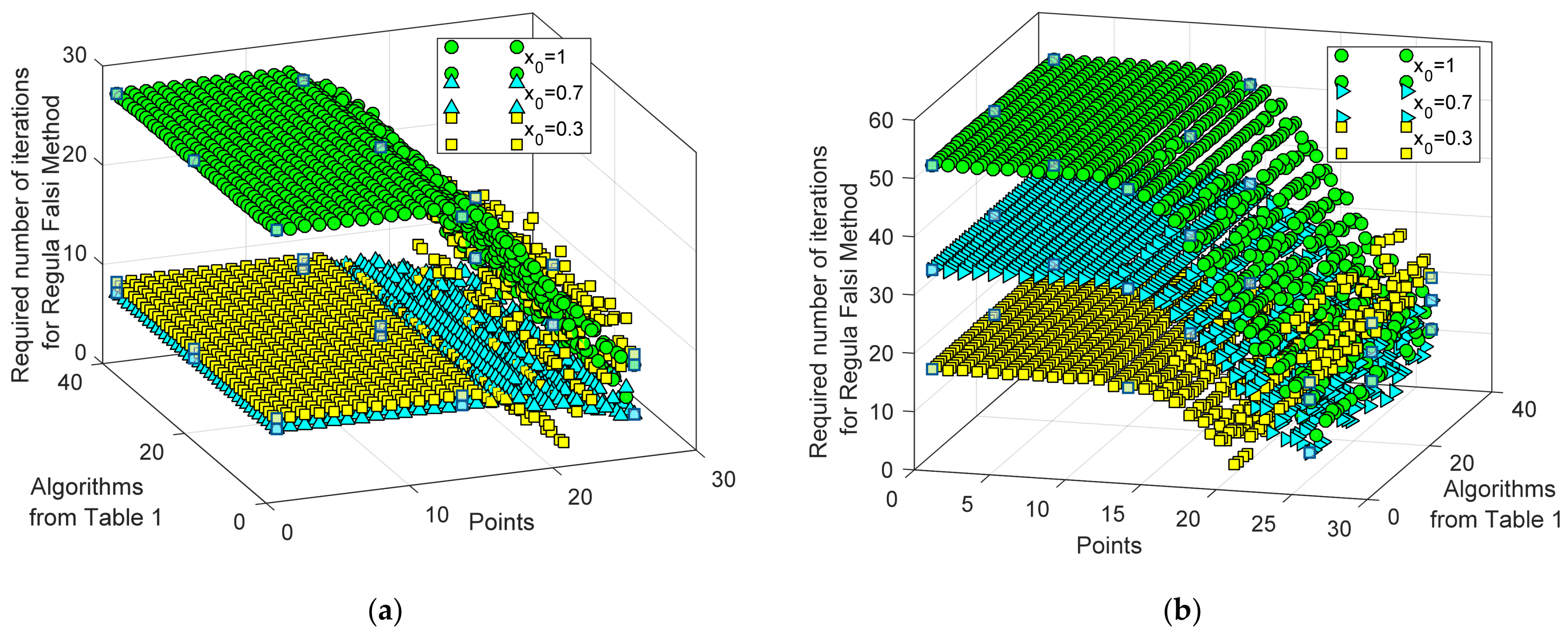
3.4. Regula Falsi Method

The Regula Falsi method (RFM), also known as the false position or false position method, is an old iterative method for solving nonlinear equations. This method is similar to the “trial and error” technique in using a test (“false”) value for the variable and then adjusting the test value according to the outcome. In SM, we may find that the difference f(x_n) − f(x_n − 1) in the denominator can become close to zero quickly. Therefore, this “risky” division by numbers close to zero can be avoided if we fix one starting point throughout the entire iterative process. Thus, an iterative formula for the RFM is:

$$x_{n+1}=x_n-\frac{x_n-x_0}{f\left(x_n\right)-f\left(x_0\right)}f\left(x_n\right).$$

(20)

The RFM has the procedure given in Algorithm 4.

Algorithm 4: Procedure of Regula Falsi method.

Define initial solution x0 and stopping criteria

Set the counter n to 1

while$abs\left({\alpha }_{DDM}+{\beta }_{DDM}{e}^{{\delta }_{DDM}\cdot x}-x{e}^x\right)>criteria$

$\begin{array}{l}{x}_{n+1}=x_n-\frac{x_n-x_0}{f\left(x_n\right)-f\left(x_0\right)}f\left(x_n\right)\\ n=n+1\end{array}$

end while

Return xn

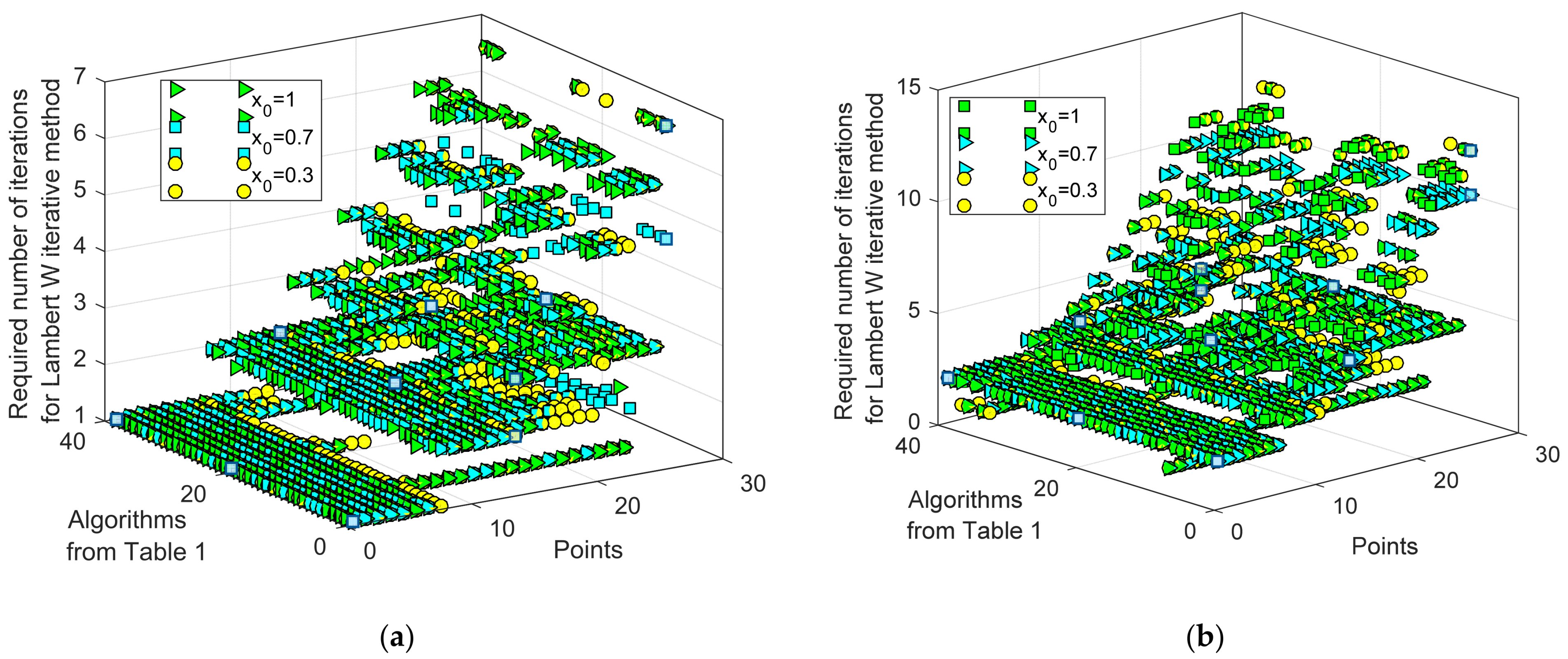
3.5. Iterative Lambert W Method

In [11,13,14], the authors proposed an iterative procedure for solving the nonlinear equation to describe current–voltage dependence based on the Lambert W function. This method is called the iterative Lambert W function (ILWF). This method relies on the fact that Equation (21) represents the Lambert W function. The mentioned equation has a solution marked as W, where W represents the solution of the equation for a known value of variable A:

$$A=x\cdot \exp \left(x\right).$$

(21)

$$x=W\left(A\right).$$

(22)

The ILWF has the procedure given in Algorithm 5

Algorithm 5: Procedure of iterative Lambert W method.

Define initial solution x0 and stopping criteria

Set the counter n to 1

while$abs\left({\alpha }_{DDM}+{\beta }_{DDM}{e}^{{\delta }_{DDM}\cdot x}-x{e}^x\right)>criteria$

$\begin{array}{l}A=\alpha +\beta \exp \left(\chi \cdot x_{n-1}\right)\\ x_n=W\left(A\right)\\ n=n+1\end{array}$

end while

Return xn

4. Numerical Results

In the literature, one can address many methods and algorithms used in estimating diode model parameters, in which the principal methods and algorithms can be categorized into numerical (deterministic and metaheuristic), analytical, and hybrid forms. The analytical methods are easy to implement but necessitate simplifications or approximations of the expressions used. The iterative-based numerical methods might provide precise solutions, but they are time-consuming in obtaining accurate global solutions because their performance is highly dependent on the initial values. Numerical-based methods may include evolutionary rules or metaheuristics, but their performance depends on adequately adjusting the control parameters. Accordingly, the authors compared their results with the most precise estimation results obtained by recent optimization algorithms from different families, with no clustering of results or selection of specific algorithms.

To test the efficiency and speed of convergence of the previously-described iterative methods used in solving the current–voltage characteristics of DDM and TDM of equivalent circuits of solar cells, one solar cell (RTC France cell) and one solar module (Photowatt-PWP201 module) were investigated. However, testing was conducted for different parameter values of these solar cells, determined by using many other methods presented in the literature. For the DDM of the RTC France solar cell, forty combinations of parameters were found in the literature and are provided in

Table 1. DDM parameters for RTC France cell.

Number	Ref.	Year	Algorithms	Ipv (A)	I01 (μA)	n1	RS (Ω)	RP (Ω)	I02 (μA)	n2
1	[12]	2022	GTO-HBA	0.7607801	0.84162	1.999999	0.03679	55.73	0.2154505	1.44706
2			HBA-GTO	0.76078	0.841611	2.00000	0.0367905	55.72835	0.2154501	1.44704
3	[14]	2021	CLSHADE	0.76076	0.2044	1.44241	0.036907	55.53	0.876400	1.99520
4	[17]	2021	LCNMSE	0.76078100	0.74933000	2.00000000	0.03674000	55.48542000	0.22598000	1.45101700
5	[18]	2021	EO	0.76792000	0.39999000	2.00000000	0.03659000	54.17614000	0.26605000	1.46451000
6	[19]	2021	WHHO	0.76078094	0.22857400	1.45189500	0.03672887	55.42643282	0.727182	2.00000
7	[20]	2021	CNMSMA	0.76078100	0.22597600	1.45101700	0.036740	55.48545	0.75068100	1.9999990
8	[21]	2021	GAMNU	0.76082700	0.32245246	1.48102800	0.03636440	53.11079000	0.00027392	1.47010100
9	[22]	2021	GSK	0.76080000	0.25950000	1.46270000	0.03660000	54.93300000	0.47910000	1.99830000
10	[23]	2021	EABOA	0.76082865	0.25072000	1.45988481	0.03662660	55.36601290	0.72069000	1.99997318
11	[24]	2020	SMA	0.76076000	0.74874000	2.00000000	0.03677	55.71456	0.22652000	1.4546300
12	[25]	2020	EOTLBO	0.76078108	0.22597468	1.45101692	0.03674043	55.48543568	0.74934431	2.0000000
13	[26]	2020	EHHO	0.760769017	0.58618400	1.968451449	0.036598831	55.63943956	0.24096500	1.456910409
14	[27]	2020	CSO	0.76080	0.22730	1.45130	0.03670	55.43270	0.73840000	1.99990
15	[28]	2020	R-II	0.76078	0.74911	2.00000	0.03675	55.71854	0.22641	1.45471
16			R-III	0.76078	0.74814	2.00000	0.03674	55.71851	0.21911	1.45145
17	[29]	2019	COA	0.76078	0.22597	1.45102	0.03674	55.48542	0.749346	2.00000
18	[30]	2019	PGJAYA	0.76080	0.21031	1.44500	0.03680	55.81350	0.885340	2.00000
19			GOTLBO	0.76080	0.13894	1.72540	0.03650	53.40580	0.262090	1.46580
20			JAYA	0.76070	0.00608	1.84360	0.03640	52.65750	0.315070	1.47880
21			STLBO	0.76080	0.23364	1.45380	0.03670	55.33820	0.684940	2.00000
22			TLABC	0.76080	0.33673	1.48610	0.03610	55.06760	0.071730	1.93160
23			CLPSO	0.76070	0.25843	1.46250	0.03670	57.94220	0.386150	1.94350
24			BLPSO	0.76080	0.27189	1.46740	0.03660	61.13450	0.435050	1.96620
25			DE/BBO	0.76060	0.00122	1.87910	0.03580	58.40180	0.372200	1.49560
26	[31]	2019	CLPSO	0.76112	0.00237	1.68481	0.03619	52.40069	0.338750	1.48612
27			BLPSO	0.76056	0.17895	1.69574	0.03553	64.79937	0.315600	1.48789
28			IJAYA	0.76079	0.49461	1.88559	0.03671	54.65515	0.220690	1.45021
29			SFS	0.76078	0.65647	1.99990	0.03669	55.30604	0.237210	1.45509
30			pSFS	0.76078	0.84161	2.00000	0.03679	55.72835	0.215450	1.44705
31	[32]	2018	FA	0.76101	0.00000	2.00000	0.03671	49.18670	0.292634	1.47134
32			HFAPS	0.76078	0.22597	1.45101	0.03674	55.48550	0.749358	2.00000
33			ABC	0.76081	0.19268	1.43800	0.03686	55.93352	0.999587	1.98372
34	[33]	2018	ELPSO	0.76081	1.00000	1.83576	0.03755	55.92047	0.099168	1.38609
35			BSA	0.76162	0.41639	1.50537	0.03539	54.45518	0.000001	2.00000
36			ABC	0.76072	0.28670	1.46915	0.03666	58.29956	0.247485	1.96837
37			GA	0.76886	0.66062	1.60874	0.02914	51.11600	0.455149	1.62890
38			ELPSO	0.76081	1.00000	1.83576	0.03755	55.92047	0.099168	1.38609
39	[34]	2017	CWOA	0.76077	0.24150	1.45651	0.03666	55.20160	0.600000	1.98990
40	[35]	2017	BPFPA	0.76000	0.32110	1.47930	0.03640	59.62400	0.045280	2.00000

, and for TDM, eleven varieties of parameters are provided in

Table 2. TDM parameters for RTC France cell.

Number	Ref.	Year	Algorithms	Ipv (A)	I01 (μA)	n1	RS (Ω)	RP (Ω)	I02 (μA)	n2	I03 (μA)	n3
1	[12]	2022	GTO-HBA	0.7607602	0.876504	1.99504	0.0369201	55.6798	0.20441	1.442401	0.0001805	1.89001
2			HBA-GTO	0.7607601	0.876499	1.99501	0.0369202	55.6801	0.204401	1.44241	0.0001801	1.89001
3	[36]	2018	ABC	0.760700	0.2000	1.4414	0.03687	55.8344	0.500000	1.90000	0.2100	2.000000
4			OBWOA	0.760770	0.2353	1.4543	0.03668	55.4448	0.221300	2.00000	0.4573	2.000000
5			STLBO	0.760800	0.2349	1.4541	0.0367	55.2641	0.229700	2.00000	0.4443	2.000000
6	[28]	2020	R-II	0.760792	0.2600	1.4608	0.03660	54.9149	0.000006	1.14660	0.5700	2.020800
7			R-III	0.760791	0.2100	1.7714	0.03670	55.3571	0.220000	1.45130	0.9900	2.410300
8			PSO	0.760782	0.2500	1.4601	0.03660	55.3133	0.041000	1.74090	1.0000	2.251400
9			CS	0.760776	0.1400	1.4872	0.03630	53.7218	0.190000	1.47710	0.0310	4.466300
10			ABC	0.760790	0.3200	1.8666	0.03670	55.4411	0.230000	1.45210	0.7400	2.394900
11			TLO	0.760763	0.2800	1.4684	0.03650	55.3821	0.000670	1.54680	1.0000	2.322500

. In the same way, for Photowatt-PWP201 modules, six parameter combinations for DDM were used and are provided in

Table 3. DDM parameters for Photowatt-PWP solar cell.

Number	Ref.	Year	Algorithms	Ipv (A)	I01 (μA)	n1	RS (Ω)	RP (Ω)	I02 (μA)	n2
1	[12]	2022	GTO-HBA	1.03242	2.5130	47.418	1.2393	744.724	3.89 × 10−6	50
2			HBA-GTO	1.0325	2.5150	47.421	1.23928	743.666	3.8885 × 10−6	49.88
3	[37]	2021	CGBO	1.0305	3.48	48.6428	1.2013	981.8874	3.89 × 10−6	34.7828
4			GBO	1.0305	3.47	48.6314	1.2016	981.2677	0	50
5	[38]	2020	EO	1.0288	9.38 × 10−4	47.1325	1.1896	1310.6705	3.96	49.1369
6	[39]	2015	IMO	1.0251	0	45.7618	1.2339	1849.8346	3.07	48.1472

. Definitions of abbreviations of the algorithms used in Table 1, Table 2 and Table 3 are given in the list of acronyms at the end of the manuscript.

To avoid confusion, the algorithms presented in the tables that have been used for solar cell parameter estimation are called “algorithms” in the results, while “methods” refers to the iterative methods used—NM, MNM, SM, RFM, and ILWF.

It should be noted that values of the parameters of solar cells in DDM and TDM are frequently shown with many digits in the literature, as shown in Table 1, Table 3 and Table 3. Thus, we solved the equations for DDM and TDM with a high degree of accuracy to align with scientific works in this field.

4.1. DDM

4.1.1. RTC France Solar Cell

The RTC France solar cell is a well-known cell in the literature, with 26 measured current–voltage pairs of points. The appearance of the equations ${\alpha }_{DDM}+{\beta }_{DDM}{e}^{{\delta }_{DDM}{y}_{DDM}}$ and $y_{DDM}{e}^{y_{DDM}}$ as well as the potential solutions for all voltage values are shown in Figure 2. As can be seen, for all voltage values, the solution of this equation is in the range from 0 to 1.

To test the efficiency of iterative methods, it was assumed that the accuracy of solving equations is 10⁻⁵ and 10⁻¹⁰, while the initial value of each of the iterative methods is x₀ = 1, x₀ = 0.7, and x₀ = 0.3. The obtained results are shown on the 3D graphs (Figure 3, Figure 4, Figure 5, Figure 6 and Figure 7). In these graphs, the x-axis represents a point from the measured voltage–current characteristic, the y-axis represents the algorithms presented in Table 1, and the z-axis represents the required number of iterations to achieve the appropriate accuracy. Based on the 3D graphics, it can be concluded that the ILWF, for almost all parameter combinations, is very efficient for small voltage values, while it requires more iterations for larger values. For a small amount of voltage, values of coefficients ${\alpha }_{DDM}$ and ${\beta }_{DDM}$ are minimal. The opposite is true for NM.

A summary of the minimum and maximum number of iterations for the iterative methods, observing all measured points of the RTC France solar cell (DDM) for all the assumed accuracies, is given in

Table 4. Minimum and maximum number of iterations for the used iterative methods observing all measured points of RTC France solar cell.

Method	Value	Stopping Criteria
		10−5			10−10
		x0 = 1	x0 = 0.7	x0 = 0.3	x0 = 1	x0 = 0.7	x0 = 0.3
NM	Min	3	1	1	4	2	2
	Max	5	5	5	6	6	6
MNM	Min	5	2	>1000	10	4	>1000
	Max	52	30		109	63
SM	Min	5	2	2	6	4	3
	Max	11	7	8	12	9	9
RFM	Min	27	2	2	9	4	3
	Max	5	17	15	52	34	28
ILWF	Min	1	1	1	1	1	1
	Max	7	6	7	13	11	13

.

Based on the graphical results and results shown in Table 4, it is clear that the MNM requires the most significant number of iterations to achieve the appropriate accuracy. This is seen for both accuracy values (10⁻¹⁰ and 10⁻⁵). After that, the most significant number of iterations is required by the RFM. The minimum number of iterations for appropriate accuracy, as seen in Table 4, are noted in the solutions obtained using the MN and the ILWF procedures.

To examine both NM and ILWF in detail, we conducted another test with an accuracy of 10⁻¹⁵, 10^−10, and 10⁻⁵ and different initial conditions. The obtained results are presented in

Table 5. Minimum and maximum number of iterations for NM and ILWF observing all measured points of RTC France solar cell.

Criteria	Method	Value	x0
			−10	1	10	100
10−5	NM	Min	>1000	3	15	107
		Max		5	16	108
	ILWF	Min	1	1	1	1
		Max	9	7	8	8
10−10	NM	Min	>1000	4	16	108
		Max		6	17	109
	ILWF	Min	1	1	1	1
		Max	14	13	14	14
10−15	NM	Min	>1000	4	16	108
		Max		7	18	110
	ILWF	Min	2	2	2	2
		Max	19	18	19	19

, as well as in Figure 8 and Figure 9. The initial values were −10, 1, 10, and 100.

It can be seen from both graphical and tabulated representations that the Lambert W iterative method has almost the same values of the required number of iterations for all values of initial conditions. Specifically, for an accuracy of 10⁻¹⁵, the maximum number of iterations is 19, and the minimum is 2. The value of the criterion is low, and the maximum and the minimum number of iterations are reduced. However, NM is highly dependent on the initial conditions. For instance, it can be seen that for an accuracy of 10⁻¹⁵, the required number of iterations at the initial value x₀ = 100 is about 110, while at x₀ = 1, the necessary number of iterations is in the range of 4 to 7. For negative initial values, the number of iterations of Newton’s method exceeds 1000.

Based on all previously presented results, it is evident that the iterative Lambert W function is more effective in solving the current–voltage equation than the other iterative methods. Additionally, to offer one more advantage of the iterative Lambert W function, Figure 10 presents the convergence curve of NM, and the ILWF determined for all values of the measured voltage and the solar cell parameters given as [0.76000 0.32110 1.47930 0.03640 59.62400 0.045280 2.00000] for case 1 and [0.7607801 0.84162 1.999999 0.03679 55.73 0.2154505 1.44706] for case 2 for [I_pv (A) I₀₁ (μA) n₁ R_S (Ω) R_P (Ω) I₀₂ (μA) n₂] for the DDM representing the RTC France solar cell. In both cases, we take x₀ = 10 and a stopping criterion 10⁻¹⁰. It is clear that ILWF gets a lower starting value of the difference ${\alpha }_{DDM}+{\beta }_{DDM}{e}^{{\delta }_{DDM}{y}_{DDM}}-y_{DDM}{e}^{y_{DDM}}$ with a high convergence speed.

4.1.2. Photowatt-PWP201 Modules

The same analysis was performed for the Photowatt-PWP201 modules. The solutions to ${\alpha }_{DDM}+{\beta }_{DDM}{e}^{{\delta }_{DDM}{y}_{DDM}}=y_{DDM}{e}^{y_{DDM}}$ for all values of voltages are presented in Figure 11. A comparison of the different methods in terms of the required number of iterations for x₀ = 1 and two values of the stopping criteria (10⁻⁵ and 10⁻¹⁰) is depicted in Figure 12.

The results presented in

Table 6. Minimum and maximum number of iterations for the iterative methods used observing all measured points of Photowatt-PWP201 modules.

Method	Value	Stopping Criteria
		10−5			10−10
		x0 = 0.9	x0 = 1.0	x0 = 1.2	x0 = 0.9	x0 = 1.0	x0 = 1.2
NM	Min	2	2	2	3	3	3
	Max	5	5	5	6	6	6
MNM	Min	2	3	3	4	5	4
	Max	64	52	73	125	109	151
SM	Min	3	3	3	4	5	4
	Max	9	11	24	10	12	25
RFM	Min	3	3	3	5	5	5
	Max	24	27	36	46	52	68
ILWF	Min	1	1	1	1	1	1
	Max	4	4	4	7	7	7

for the five iterative methods and the initial values of x₀ = 0.9, x₀ = 1, and x₀ = 1.2 for the DDM of the Photowatt-PWP201 modules correspond to the results shown for the RTC France solar cell in Table 4. An additional comparison between NM and ILWF for x₀ = 10, x₀ = 50, and x₀ = 100 is also presented in

Table 7. Minimum and maximum number of iterations for NM and ILWF observing all the measured points of Photowatt-PWP201 module.

Criteria	Method	Value	x0
			10	50	100
10−5	NM	Min	14	56	106
		Max	16	58	108
	ILWF	Min	1	1	1
		Max	5	6	6
10−10	NM	Min	15	57	107
		Max	17	59	109
	ILWF	Min	1	1	1
		Max	8	9	9

.

The dependence of the required number of iterations for Newton and iterative Lambert W function for 10⁻⁵ and different initial values (x₀ = 10, x₀ = 50, and x₀ = 100) is presented in Figure 13.

The modified Newton method requires the most significant number of iterations to achieve appropriate accuracy, followed by the Regula Falsi and Secant methods. In contrast, the Newton and Iterative Lambert W methods need the smallest number of iterations. However, the iterative Lambert W method is almost independent of the initial conditions, as shown in Figure 13.

Additionally, to present one more advantage of the Iterative Lambert W function, Figure 14 shows the convergence curve of Newton’s method and the Iterative Lambert W method determined for all values of the measured voltage and the solar cell parameters [1.0251 0 45.7618 1.2339 1849.8346 3.07 48.1472] for [I_pv (A) I₀₁ (μA) n₁ R_S (Ω) R_P (Ω) I₀₂ (μA) n₂] for the DDM representing the solar Photowatt-PWP201 module. In this case, we take x₀ = 10 and a stopping criterion set to 10⁻¹⁰. Clearly, the iterative Lambert W function obtains the lower starting value of difference ${\alpha }_{DDM}+{\beta }_{DDM}{e}^{{\delta }_{DDM}{y}_{DDM}}-y_{DDM}{e}^{y_{DDM}}$ and its convergence speed is higher than that obtained using Newton’s method.

4.2. TDM

The tested algorithms’ efficiency was also performed for Equation (2), which represents the TDM of solar cells. In this regard, the RTC France solar cell was observed once again. Visualization of the equations ${\alpha }_{TDM}+{\beta }_{TDM}{e}^{{\delta }_{TDM}{y}_{TDM}}+{\gamma }_{TDM}{e}^{{\sigma }_{TDM}{y}_{TDM}}$ and $y_{TDM}{e}^{y_{TDM}}$ as well as the potential solution for all the voltage values are shown in Figure 15. It can be seen that the solution to this equation is in the range from 0 to 1 for all voltage values.

For much more efficient testing, several combinations of parameters of this solar cell of the reviewed scientific publications dealing with estimating the parameters of these cells were considered. The obtained results are shown in Figure 16 and Figure 17. Figure 16 shows the required number of iterations for each addressed method, considering that the accuracy of solving Equation (2) is 10⁻⁵, while the initial values of the functions are 1, 0.7, and 0.5, respectively. The corresponding results for the accuracy of solving equations 10⁻¹⁰ are shown in Figure 17. In both figures, the results for MNM for the initial value of 0.5 are not shown, because the maximum number of iterations is extremely large.

A summary of the minimum and maximum number of iterations for the iterative methods, observing all measured points of RTC France solar cell (TDM) for all the assumed accuracies and initial conditions, is given in

Table 8. Minimum and maximum number of iterations for the used iterative methods observing the measured points of the TDM representing the RTC France solar cell.

Method	Value	Stopping Criteria
		10−5			10−10
		x0 = 1.0	x0 = 0.7	x0 = 0.5	x0 = 1.0	x0 = 0.7	x0 = 0.5
NM	Min	5	2	2	4	3	3
	Max	3	5	4	6	6	5
MNM	Min	5	2	2	10	5	4
	Max	52	30	1783	109	63	3792
SM	Min	5	3	3	6	5	4
	Max	11	7	7	12	9	8
RFM	Min	5	3	3	9	6	5
	Max	27	17	12	52	34	25
ILWF	Min	1	1	1	2	2	2
	Max	7	6	6	13	11	12

.

Based on the presented results, the efficiency of the Newton and iterative Lambert W methods is precise. Therefore, the presented results show the same conclusions drawn for DDM solar cells.

A detailed comparison of Newton’s and iterative Lambert W methods was also performed for larger initial values. The results obtained are shown in Figure 18 and Figure 19 for two different stopping criteria. Additionally, a summary of the results in terms of maximum and minimum iteration numbers is shown in

Table 9. Minimum and maximum number of iterations for NM and ILWF observing all the measured points of the TDM representing the RTC France solar cell.

Criteria	Method	Value	x0
			10	50	100
10−5	NM	Min	15	56	107
		Max	16	58	108
	ILWF	Min	1	1	1
		Max	8	8	8
10−10	NM	Min	16	57	108
		Max	17	59	109
	ILWF	Min	2	2	2
		Max	14	14	14

. The obtained results, as in the case of DDM, validate the efficiency of applying the iterative Lambert W method. Moreover, the iterative Lambert W function is almost independent of the initial values, even in the case of large initial values.

Additionally, to present one more advantage of the iterative Lambert W function, Figure 20 shows the convergence curve of Newton’s and iterative Lambert W methods determined for all values of the measured voltage and the following solar cell parameters [0.760763 0.2800 1.4684 0.03650 55.3821 0.000670 1.54680 1.0000 2.322500] for [I_pv (A) I₀₁ (μA) n₁ R_S (Ω) R_P (Ω) I₀₂ (μA) n₂ I₀₃ (μA) n₃] of the TDM representing the RTC France solar cell. In this case, we take x₀ = 10 and a stopping criterion = 10⁻¹⁰.

It is clear that the iterative Lambert W function obtains a low starting value of difference ${\alpha }_{DDM}+{\beta }_{DDM}{e}^{{\delta }_{DDM}{y}_{DDM}}-y_{DDM}{e}^{y_{DDM}}$ and the convergence speed is high. Finally, it is necessary to give an overview of the time consumed in iterations of all the tested methods. First, the SM does not require searching for a derivative function or some social function and is, therefore, the least time-consuming method. The same conclusion applies to the RFM method. The MNM requires looking for a function’s derivative at the first point, while later, during iterations, this value is used. If the function is differentiable, which is the case in this work, then the value of the derivative is determined relatively easily and quickly.

NM necessitates differentiating the function in each iteration. This operation is not time-consuming if the function is differentiable. However, with the NM, the value of the derivative of the function changes in each iteration. Finally, the ILWF is based on solving the Lambert W function in each iteration. The Lambert W function can be solved in several ways—analytically (by applying the special trans function theory (STFT) used in finding the exact analytical closed-form solution in some detail), developing the function in Raylor’s order, or iteratively (using any iterative method). However, today’s software packages such as MATLAB, Mathematica, Maple, and others have a built-in function to solve the Lambert W function. Therefore, ILWF relies on the time required to solve this function, which depends on the computer used. Thus, the ILWF is the most time-consuming method, followed by NM, MNM, RFM, and SM. The specific speed ratio between them depends on the speed of the computer used, available memory, and the speed of the processor.

5. Conclusions

Solar energy is one of the most promising renewable energy sources. Therefore, reliable, efficient, accurate, and fast modeling of solar power plants and their components is essential. This paper investigated the efficiency of the application of different iterative methods for solving current–voltage dependencies in double diode and triple diode models of solar cells.

To this end, four iterative methods and one advanced iterative method based on the Lambert W function were tested. All tests were performed using different accuracies of solving the highly nonlinear current–voltage equation and using different initial conditions. In addition, the time requirements of each of the methods were addressed. It has been shown that the Lambert W function and Newton’s method (for specific values of the initial value) led to excellent efficiency in solving the current–voltage dependence, compared to the other methods. In this regard, the iterative Lambert W function was almost independent of the initial conditions, which is an excellent advantage over Newton’s method. Tests were performed for different parameters of the well-known RTC France solar cell and Photowatt-PWP module used in many research works for the triple and double diode models. Finally, this work will further lead us to better develop equivalent solar cell models, their mathematical representation, and the optimization methods used to estimate their parameters. In future works, we will focus on developing new iterative algorithms that combine the good properties of the investigated methods.

References

1. Premkumar, M.; Karthick, K.; Sowmya, R. A Review on Solar PV Based Grid Connected Microinverter Control Schemes and Topologies. Int. J. Renew. Energy Dev. 2018, 7, 171. [Google Scholar] [CrossRef]
2. Ali, Z.M.; Diaaeldin, I.M.; Abdel Aleem, S.H.E.; El-Rafei, A.; Abdelaziz, A.Y.; Jurado, F. Scenario-Based Network Reconfiguration and Renewable Energy Resources Integration in Large-Scale Distribution Systems Considering Parameters Uncertainty. Mathematics 2021, 9, 26. [Google Scholar] [CrossRef]
3. Saric, M.; Hivziefendic, J.; Konjic, T.; Ktena, A. Distributed Generation Allocation Considering Uncertainties. Int. Trans. Electr. Energy Syst. 2018, 28, e2585. [Google Scholar] [CrossRef]
4. Ali, Z.M.; Diaaeldin, I.M.; El-Rafei, A.; Hasanien, H.M.; Abdel Aleem, S.H.E.; Abdelaziz, A.Y. A Novel Distributed Generation Planning Algorithm via Graphically-Based Network Reconfiguration and Soft Open Points Placement Using Archimedes Optimization Algorithm. Ain Shams Eng. J. 2021, 12, 1923–1941. [Google Scholar] [CrossRef]
5. Mostafa, M.H.; Abdel Aleem, S.H.E.; Ali, S.G.; Abdelaziz, A.Y. Energy-Management Solutions for Microgrids. In Distributed Energy Resources in Microgrids: Integration, Challenges and Optimization; Elsevier: Amsterdam, The Netherlands, 2019; pp. 483–515. [Google Scholar]
6. Almalaq, A.; Alqunun, K.; Refaat, M.M.; Farah, A.; Benabdallah, F.; Ali, Z.M.; Aleem, S.H.E.A. Towards Increasing Hosting Capacity of Modern Power Systems through Generation and Transmission Expansion Planning. Sustainability 2022, 14, 2998. [Google Scholar] [CrossRef]
7. Ćalasan, M.; Abdel Aleem, S.H.E.; Bulatović, M.; Rubežić, V.; Ali, Z.M.; Micev, M. Design of Controllers for Automatic Frequency Control of Different Interconnection Structures Composing of Hybrid Generator Units Using the Chaotic Optimization Approach. Int. J. Electr. Power Energy Syst. 2021, 129, 106879. [Google Scholar] [CrossRef]
8. Lukačević, O.; Almalaq, A.; Alqunun, K.; Farah, A.; Ćalasan, M.; Ali, Z.M.; Abdel Aleem, S.H.E. Optimal CONOPT Solver-Based Coordination of Bi-Directional Converters and Energy Storage Systems for Regulation of Active and Reactive Power Injection in Modern Power Networks. Ain Shams Eng. J. 2022, 13, 101803. [Google Scholar] [CrossRef]
9. Rawa, M.; Al-Turki, Y.; Sindi, H.; Ćalasan, M.; Ali, Z.M.; Abdel Aleem, S.H.E. Current-Voltage Curves of Planar Heterojunction Perovskite Solar Cells—Novel Expressions Based on Lambert W Function and Special Trans Function Theory. J. Adv. Res. 2022; in press. [Google Scholar] [CrossRef]
10. Gnetchejo, P.J.; Ndjakomo Essiane, S.; Ele, P.; Wamkeue, R.; Mbadjoun Wapet, D.; Perabi Ngoffe, S. Important Notes on Parameter Estimation of Solar Photovoltaic Cell. Energy Convers. Manag. 2019, 197, 111870. [Google Scholar] [CrossRef]
11. Ćalasan, M.; Abdel Aleem, S.H.E.; Zobaa, A.F. On the Root Mean Square Error (RMSE) Calculation for Parameter Estimation of Photovoltaic Models: A Novel Exact Analytical Solution Based on Lambert W Function. Energy Convers. Manag. 2020, 210, 112716. [Google Scholar] [CrossRef]
12. Rawa, M.; Abusorrah, A.; Al-Turki, Y.; Calasan, M.; Micev, M.; Ali, Z.M.; Mekhilef, S.; Bassi, H.; Sindi, H.; Aleem, S.H.E.A. Estimation of Parameters of Different Equivalent Circuit Models of Solar Cells and Various Photovoltaic Modules Using Hybrid Variants of Honey Badger Algorithm and Artificial Gorilla Troops Optimizer. Mathematics 2022, 10, 1057. [Google Scholar] [CrossRef]
13. Rawa, M.; Calasan, M.; Abusorrah, A.; Alhussainy, A.A.; Al-Turki, Y.; Ali, Z.M.; Sindi, H.; Mekhilef, S.; Aleem, S.H.E.A.; Bassi, H. Single Diode Solar Cells—Improved Model and Exact Current–Voltage Analytical Solution Based on Lambert’s W Function. Sensors 2022, 22, 4173. [Google Scholar] [CrossRef] [PubMed]
14. Ćalasan, M.; Abdel Aleem, S.H.E.; Zobaa, A.F. A New Approach for Parameters Estimation of Double and Triple Diode Models of Photovoltaic Cells Based on Iterative Lambert W Function. Sol. Energy 2021, 218, 392–412. [Google Scholar] [CrossRef]
15. Araújo, N.M.F.T.S.; Sousa, F.J.P.; Costa, F.B. Equivalent models for photovoltaic cell—A review. Sci. Eng. 2020, 19, 77–98. [Google Scholar] [CrossRef]
16. Conte, S.D.; de Boor, C. Elementary Numerical Analysis; Society for Industrial and Applied Mathematics: Philadelphia, PA, USA, 2017. [Google Scholar]
17. Weng, X.; Heidari, A.A.; Liang, G.; Chen, H.; Ma, X.; Mafarja, M.; Turabieh, H. Laplacian Nelder-Mead Spherical Evolution for Parameter Estimation of Photovoltaic Models. Energy Convers. Manag. 2021, 243, 114223. [Google Scholar] [CrossRef]
18. Ndi, F.E.; Perabi, S.N.; Ndjakomo, S.E.; Ondoua Abessolo, G.; Mengounou Mengata, G. Estimation of Single-Diode and Two Diode Solar Cell Parameters by Equilibrium Optimizer Method. Energy Rep. 2021, 7, 4761–4768. [Google Scholar] [CrossRef]
19. Naeijian, M.; Rahimnejad, A.; Ebrahimi, S.M.; Pourmousa, N.; Gadsden, S.A. Parameter Estimation of PV Solar Cells and Modules Using Whippy Harris Hawks Optimization Algorithm. Energy Rep. 2021, 7, 4047–4063. [Google Scholar] [CrossRef]
20. Liu, Y.; Heidari, A.A.; Ye, X.; Liang, G.; Chen, H.; He, C. Boosting Slime Mould Algorithm for Parameter Identification of Photovoltaic Models. Energy 2021, 234, 121164. [Google Scholar] [CrossRef]
21. Saadaoui, D.; Elyaqouti, M.; Assalaou, K.; ben hmamou, D.; Lidaighbi, S. Parameters Optimization of Solar PV Cell/Module Using Genetic Algorithm Based on Non-Uniform Mutation. Energy Convers. Manag. X 2021, 12, 100129. [Google Scholar] [CrossRef]
22. Xiong, G.; Li, L.; Mohamed, A.W.; Yuan, X.; Zhang, J. A New Method for Parameter Extraction of Solar Photovoltaic Models Using Gaining–Sharing Knowledge Based Algorithm. Energy Rep. 2021, 7, 3286–3301. [Google Scholar] [CrossRef]
23. Long, W.; Wu, T.; Xu, M.; Tang, M.; Cai, S. Parameters Identification of Photovoltaic Models by Using an Enhanced Adaptive Butterfly Optimization Algorithm. Energy 2021, 229, 120750. [Google Scholar] [CrossRef]
24. Kumar, C.; Raj, T.D.; Premkumar, M.; Raj, T.D. A New Stochastic Slime Mould Optimization Algorithm for the Estimation of Solar Photovoltaic Cell Parameters. Optik 2020, 223, 165277. [Google Scholar] [CrossRef]
25. Xiong, G.; Zhang, J.; Shi, D.; Zhu, L.; Yuan, X. Parameter Extraction of Solar Photovoltaic Models with an Either-or Teaching Learning Based Algorithm. Energy Convers. Manag. 2020, 224, 113395. [Google Scholar] [CrossRef]
26. Jiao, S.; Chong, G.; Huang, C.; Hu, H.; Wang, M.; Heidari, A.A.; Chen, H.; Zhao, X. Orthogonally Adapted Harris Hawks Optimization for Parameter Estimation of Photovoltaic Models. Energy 2020, 203, 117804. [Google Scholar] [CrossRef]
27. Gude, S.; Jana, K.C. Parameter Extraction of Photovoltaic Cell Using an Improved Cuckoo Search Optimization. Sol. Energy 2020, 204, 280–293. [Google Scholar] [CrossRef]
28. Premkumar, M.; Babu, T.S.; Umashankar, S.; Sowmya, R. A New Metaphor-Less Algorithms for the Photovoltaic Cell Parameter Estimation. Optik 2020, 208, 164559. [Google Scholar] [CrossRef]
29. Ćalasan, M.; Jovanović, D.; Rubežić, V.; Mujović, S.; Dukanović, S. Estimation of Single-Diode and Two-Diode Solar Cell Parameters by Using a Chaotic Optimization Approach. Energies 2019, 12, 4209. [Google Scholar] [CrossRef]
30. Yu, K.; Qu, B.; Yue, C.; Ge, S.; Chen, X.; Liang, J. A Performance-Guided JAYA Algorithm for Parameters Identification of Photovoltaic Cell and Module. Appl. Energy 2019, 237, 241–257. [Google Scholar] [CrossRef]
31. Chen, X.; Yue, H.; Yu, K. Perturbed Stochastic Fractal Search for Solar PV Parameter Estimation. Energy 2019, 189, 116247. [Google Scholar] [CrossRef]
32. Beigi, A.M.; Maroosi, A. Parameter Identification for Solar Cells and Module Using a Hybrid Firefly and Pattern Search Algorithms. Sol. Energy 2018, 171, 435–446. [Google Scholar] [CrossRef]
33. Rezaee Jordehi, A. Enhanced Leader Particle Swarm Optimisation (ELPSO): An Efficient Algorithm for Parameter Estimation of Photovoltaic (PV) Cells and Modules. Sol. Energy 2018, 159, 78–87. [Google Scholar] [CrossRef]
34. Oliva, D.; Abd El Aziz, M.; Ella Hassanien, A. Parameter Estimation of Photovoltaic Cells Using an Improved Chaotic Whale Optimization Algorithm. Appl. Energy 2017, 200, 141–154. [Google Scholar] [CrossRef]
35. Ram, J.P.; Babu, T.S.; Dragicevic, T.; Rajasekar, N. A New Hybrid Bee Pollinator Flower Pollination Algorithm for Solar PV Parameter Estimation. Energy Convers. Manag. 2017, 135, 463–476. [Google Scholar] [CrossRef]
36. Abd Elaziz, M.; Oliva, D. Parameter Estimation of Solar Cells Diode Models by an Improved Opposition-Based Whale Optimization Algorithm. Energy Convers. Manag. 2018, 171, 1843–1859. [Google Scholar] [CrossRef]
37. Premkumar, M.; Jangir, P.; Ramakrishnan, C.; Nalinipriya, G.; Alhelou, H.H.; Kumar, B.S. Identification of Solar Photovoltaic Model Parameters Using an Improved Gradient-Based Optimization Algorithm with Chaotic Drifts. IEEE Access 2021, 9, 62347–62379. [Google Scholar] [CrossRef]
38. Abdel-Basset, M.; Mohamed, R.; Mirjalili, S.; Chakrabortty, R.K.; Ryan, M.J. Solar Photovoltaic Parameter Estimation Using an Improved Equilibrium Optimizer. Sol. Energy 2020, 209, 694–708. [Google Scholar] [CrossRef]
39. Javidy, B.; Hatamlou, A.; Mirjalili, S. Ions Motion Algorithm for Solving Optimization Problems. Appl. Soft Comput. 2015, 32, 72–79. [Google Scholar] [CrossRef]
40. Kumar, S.; Kumar, D.; Sharma, J.R.; Jäntschi, L. A Family of Derivative Free Optimal Fourth Order Methods for Computing Multiple Roots. Symmetry 2020, 12, 1969. [Google Scholar] [CrossRef]
41. Kumar, S.; Kumar, D.; Sharma, J.R.; Cesarano, C.; Agarwal, P.; Chu, Y.-M. An Optimal Fourth Order Derivative Free Numerical Algorithm for Multiple Roots. Symmetry 2020, 12, 1038. [Google Scholar] [CrossRef]
42. Sharma, J.R.; Kumar, S.; Jäntschi, L. On Derivative Free Multiple-Root Finders with Optimal Fourth Order Convergence. Mathematics 2020, 8, 1091. [Google Scholar] [CrossRef]
43. Sharma, J.R.; Kumar, S.; Jäntschi, L. On a Class of Optimal Fourth Order Multiple Root Solvers without Using Derivatives. Symmetry 2019, 11, 1452. [Google Scholar] [CrossRef] [Green Version]
Figure 1. Equivalent circuit models of solar cells: (a) DDM; (b) TDM.
Mathematics 10 03082 g001
Figure 2. Visualization of α D D M + β D D M e δ D D M y D D M and y D D M e y D D M .
Mathematics 10 03082 g002
Figure 3. Required number of iterations for all voltage values with different stopping criteria using NM: (a) 10−5; (b) 10−10.
Mathematics 10 03082 g003
Figure 4. Required number of iterations for all voltage values with different stopping criteria using MNM: (a) 10−5; (b) 10−10.
Mathematics 10 03082 g004
Figure 5. Required number of iterations for all voltage values with different stopping criteria using SM: (a) 10−5; (b) 10−10.
Mathematics 10 03082 g005
Figure 6. Required number of iterations for all voltage values with different stopping criteria using RFM: (a) 10−5; (b) 10−10.
Mathematics 10 03082 g006
Figure 7. Required number of iterations for all voltage values with different stopping criteria using ILWF: (a) 10−5; (b) 10−10.
Mathematics 10 03082 g007
Figure 8. Required number of iterations for all voltage values with different stopping criteria using NM: (a) 10−5; (b) 10−10; (c) 10−15.
Mathematics 10 03082 g008
Figure 9. Required number of iterations for all voltage values with different stopping criteria using ILWF: (a) 10−5; (b) 10−10; (c) 10−15.
Mathematics 10 03082 g009aMathematics 10 03082 g009b
Figure 10. Convergence curves for NM and the ILWF for all values of the measured voltage: (a) Case 1; (b) Case 2.
Mathematics 10 03082 g010
Figure 11. Visualization of α D D M + β D D M e δ D D M y D D M and y D D M e y D D M .
Mathematics 10 03082 g011
Figure 12. Comparison of the different methods investigated in terms of the required number of iterations for x0 = 1 with two stopping criteria: (a) 10−5; (b) 10−10.
Mathematics 10 03082 g012
Figure 13. Required number of iterations for all voltage values for a stopping criterion set to 10−5 using: (a) NM; (b) ILWF.
Mathematics 10 03082 g013
Figure 14. Convergence curves for NM and the ILWF for all values of the measured voltage of the solar Photowatt-PWP201 module.
Mathematics 10 03082 g014
Figure 15. Visualization of α T D M + β T D M e δ T D M y T D M + γ T D M e σ T D M y T D M and y T D M e y T D M .
Mathematics 10 03082 g015
Figure 16. Required number of iterations for all voltage values with 10−5 stopping criterion using the five iterative methods: (a) x0 = 1; (b) x0 = 0.7; (c) x0 = 0.5.
Mathematics 10 03082 g016
Figure 17. Required number of iterations for all voltage values with 10−10 stopping criterion using the five iterative methods: (a) x0 = 1; (b) x0 = 0.7; (c) x0 = 0.5.
Mathematics 10 03082 g017
Figure 18. Required number of iterations for all voltage values with 10−5 stopping criterion using Newton’s and iterative Lambert W methods: (a) x0 = 10; (b) x0 = 50; (c) x0 = 100.
Mathematics 10 03082 g018
Figure 19. Required number of iterations for all voltage values with 10−10 stopping criterion using Newton’s and iterative Lambert W methods: (a) x0 = 10; (b) x0 = 50; (c) x0 = 100.
Mathematics 10 03082 g019
Figure 20. Convergence curves for NM and the ILWF for all values of the measured voltage of the RTC France solar cell.
Mathematics 10 03082 g020