
Detection and Analysis of Critical Dynamic Properties of Oligodendrocyte Differentiation


Abstract
:1. Introduction
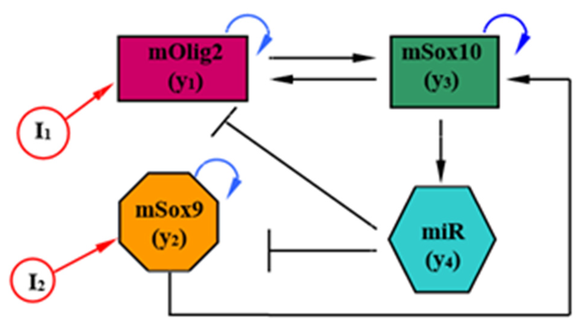
2. Model
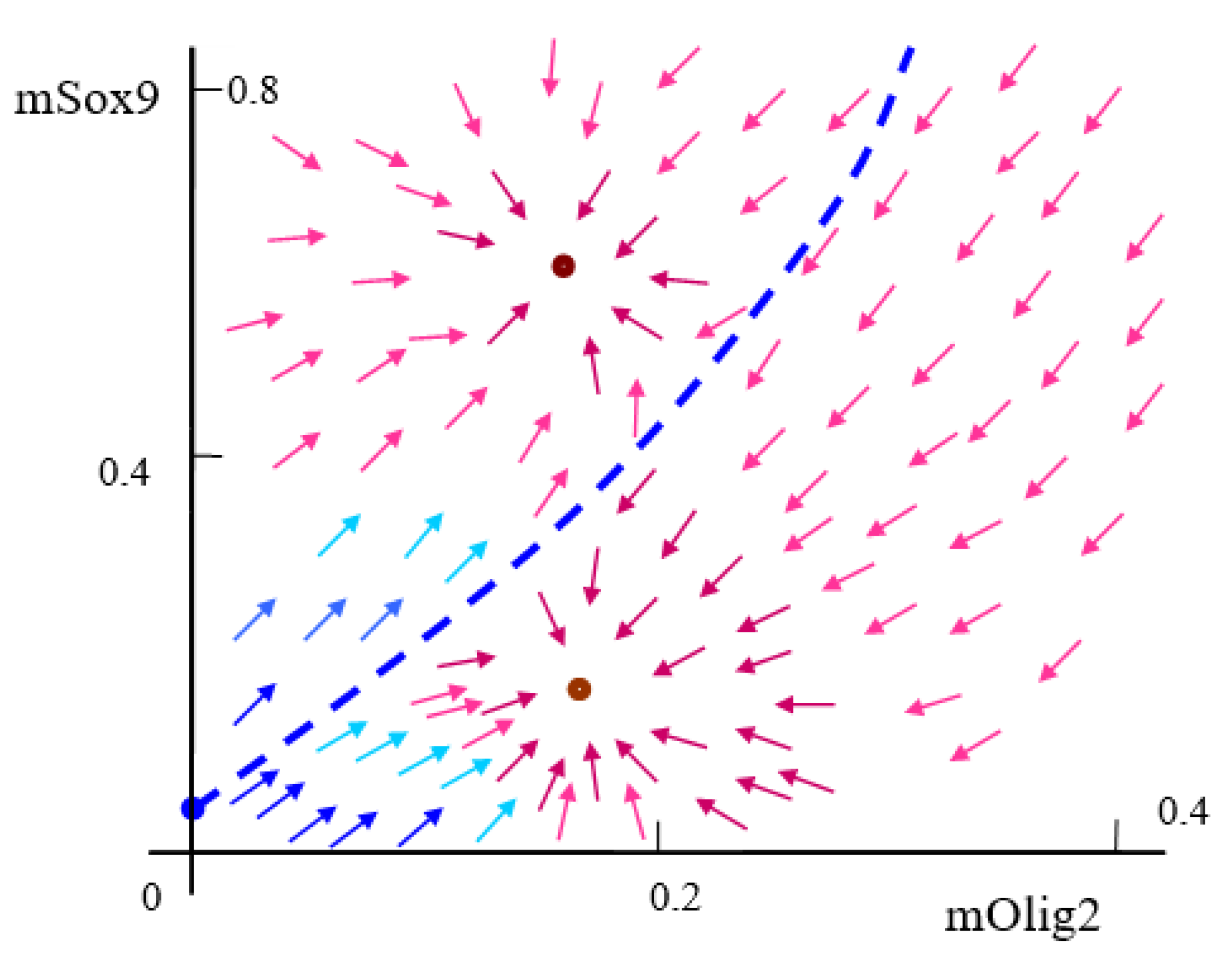
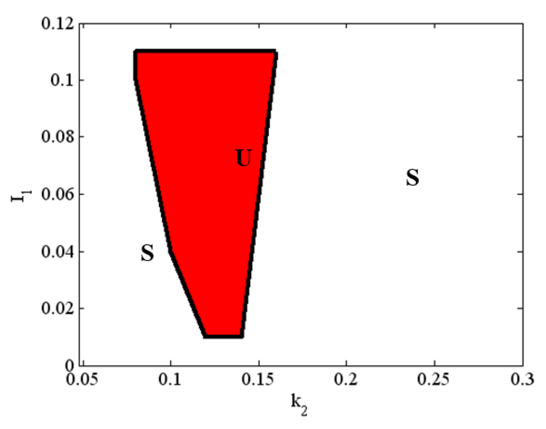
3. Qualitative Analysis and Predictions
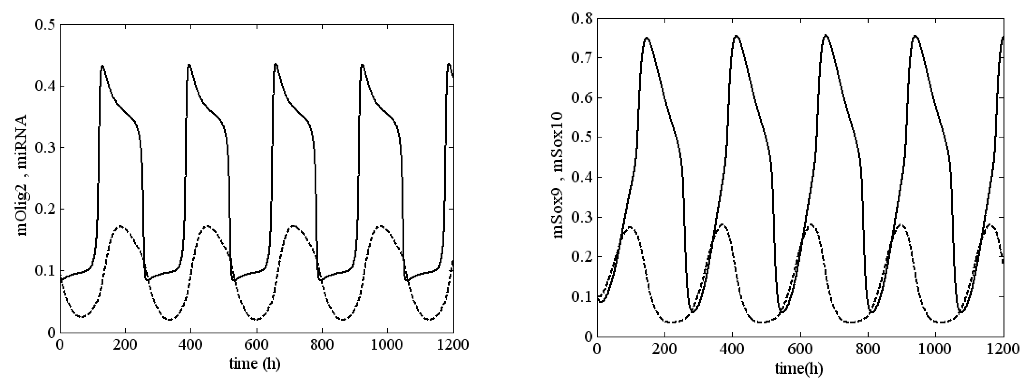
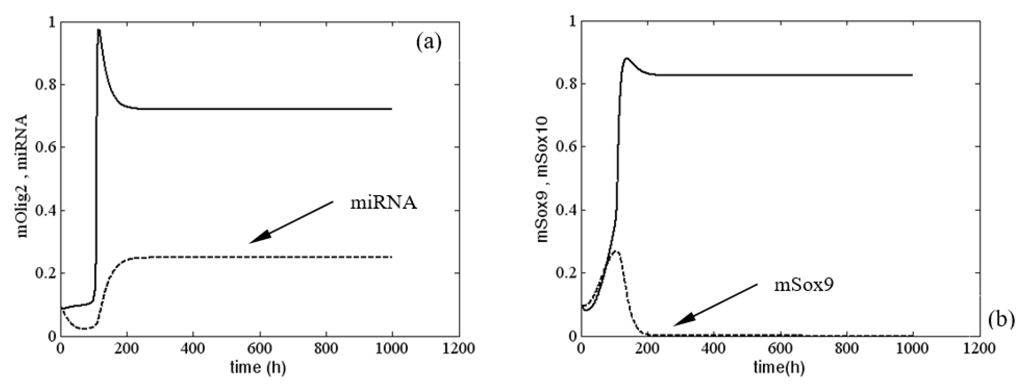
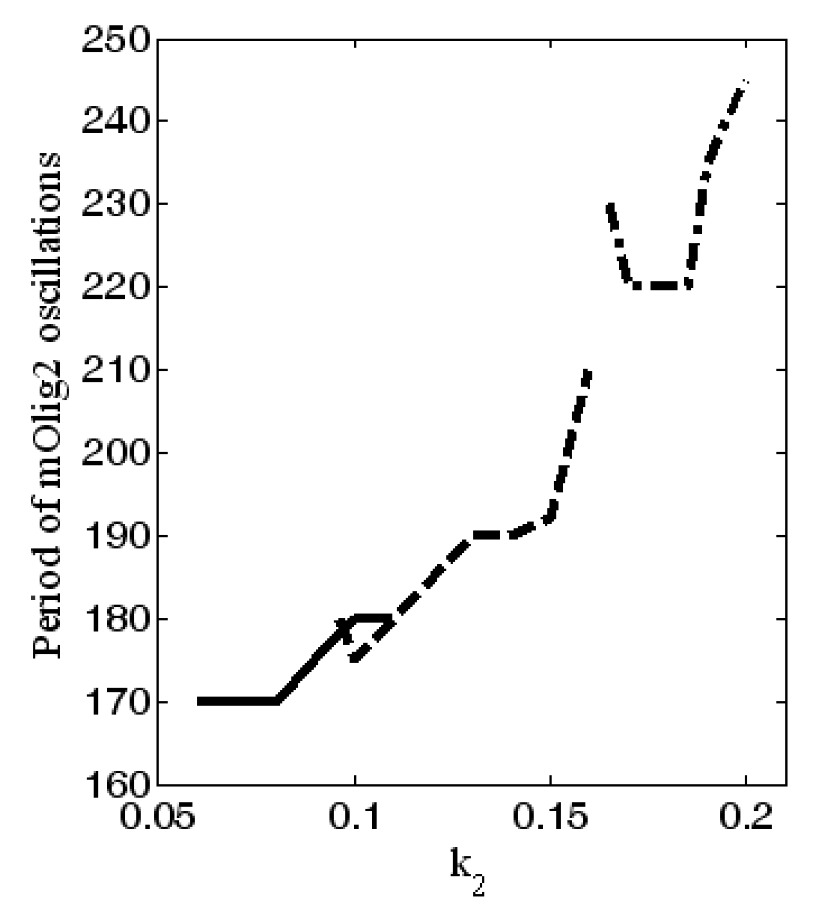
4. Numerical Investigation
5. Discussion and Conclusions
Author Contributions
Funding
Institutional Review Board Statement
Informed Consent Statement
Data Availability Statement
Conflicts of Interest
Appendix A. Qualitative Analysis: Fixed Points (Equilibrium States) Derivation
Appendix B. Calculation of
Appendix C. Qualitative Picture When Morphogen Gradients Are Equal to Zero
Appendix D. Numerical Results for System (1) When the Bifurcation Parameters and Have Different Values

References
- Luo, L. Principles of Neurobiology, 2nd ed.; CRC Press: Boca Raton, FL, USA, 2021. [Google Scholar]
- Waxman, S.G.; Bennett, M.V.L. Relative conduction velocities of small myelinated and non-myelinated fibres in the central nervous system. Nat. New Biol. 1972, 238, 217–219. [Google Scholar] [CrossRef]
- Bradl, M.; Lassman, H. Oligodendrocytes: Biology and pathology. Acta Neuropathol. 2010, 119, 37–53. [Google Scholar] [CrossRef] [PubMed]
- Kuhn, S.; Gritti, L.; Crooks, D.; Dombrowski, Y. Oligodendrocytes in development, myelin generation and beyond. Cells 2019, 8, 1424. [Google Scholar] [CrossRef] [PubMed]
- Bergles, D.; Richardson, W. Oligodendrocyte development and plasticity. Cold Spring Harb. Perspect. Biol. 2016, 8, a020453. [Google Scholar] [CrossRef] [PubMed]
- Santos, A.; Vieira, M.; Vasconcellos, R.; Goulart, V.; Kihara, A.; Resende, R. Decoding cell signaling and regulation of oligodendrocyte differentiation. Semin. Cell Dev. Biol. 2019, 95, 54–73. [Google Scholar] [CrossRef] [PubMed]
- Dufour, A.; Gontran, E.; Deroulers, C.; Varlet, P.; Pallud, J.; Grammaticos, B.; Badoual, M. Modeling the dynamics of oligodendrocyte precursor cells and the genesis of gliomas. PLOS Comput. Biol. 2018, 14, e1005977. [Google Scholar] [CrossRef] [PubMed]
- Yeung, M.S.Y.; Djelloul, M.; Steiner, E.; Bernard, S.; Salehpour, M.; Possnert, G.; Brundin, L.; Frisén, J. Dynamics of oligodenrocyte generation in multiple sclerosis. Nature 2019, 556, 538–542. [Google Scholar] [CrossRef] [PubMed]
- Swiss, V.A.; Nguyen, T.; Dugas, J.; Ibrahim, A.; Barres, B.; Androulakis, I.P.; Casaccia, P. Identification of a Gene Regulatory Network Necessary for the Initiation of Oligodendrocyte Differentiation. PLoS ONE 2011, 6, e18088. [Google Scholar] [CrossRef] [PubMed]
- Wittstatt, J.; Weider, M.; Wegner, M.; Reiprich, S. MicroRNA miR-204 regulates proliferation and differentiation of oligodendroglia in culture. Glia 2020, 68, 2015–2027. [Google Scholar] [CrossRef] [PubMed]
- Wedel, M.; Fröb, F.; Elsesser, O.; Wittmann, M.-T.; Lie, D.C.; Reis, A.; Wegner, M. Transcription factor Tcf4 is the preferred heterodimerization partner for Olig2 in oligodendrocytes and required for differentiation. Nucleic Acids Res. 2020, 48, 4839–4857. [Google Scholar] [CrossRef]
- Reiprich, S.; Cantone, M.; Weider, M.; Baroti, T.; Wittstatt, J.; Schmitt, C.; Küspert, M.; Vera, J.; Wegner, M. Transcription factor Sox10 regulates oligodendroglial Sox9 levels via microRNAs. Glia 2017, 65, 1089–1102. [Google Scholar] [CrossRef] [PubMed]
- He, D.; Marie, C.; Zhao, C.; Kim, B.; Wang, J.; Deng, Y.; Clavairoly, A.; Frah, M.; Wang, H.; He, X.; et al. Chd7 cooperates with Sox10 and regulates the onset of CNS myelination and remyelination. Nat. Neurosci. 2016, 19, 678–689. [Google Scholar] [CrossRef] [PubMed]
- Cantone, M.; Küspert, M.; Reiprich, S.; Lai, X.; Eberhardt, M.; Göttle, P.; Beyer, F.; Azim, K.; Küry, P.; Wegner, M.; et al. A gene regulatory architecture that controls region-independent dynamics of oligodendrocyte differentiation. Glia 2019, 67, 825–843. [Google Scholar] [CrossRef] [PubMed]
- Aprato, J.; Sock, E.; Weider, M.; Elsesser, O.; Fröb, F.; Wegner, M. Myrf guides target gene selection of transcription factor Sox10 during oligodendroglial development. Nucleic Acids Res. 2020, 48, 1254–1270. [Google Scholar] [CrossRef]
- Uriu, K. Genetic oscillators in development. Dev. Growth Differ. 2016, 58, 16–30. [Google Scholar] [CrossRef] [PubMed]
- Meeuse, M.W.; Hauser, Y.P.; Morales Moya, L.J.; Hendriks, G.J.; Eglinger, J.; Bogaarts, G.; Tsiairis, C.; Großhans, H. Developmental function and state transitions of a gene expression oscillator in Caenorhabditis elegans. Mol. Syst. Biol. 2020, 16, e9498. [Google Scholar] [CrossRef] [PubMed]
- Tsiaris, C.; Aulehla, A. Self-organization of embryonic genetic oscillators into spatiotemporal wave patterns. Cell 2016, 164, 656–667. [Google Scholar] [CrossRef] [PubMed]
- Sueda, R.; Kageyama, R. Oscilatory expression of Ascl1 in oligodendrogenesis. Gene Expr. Patterns 2021, 41, 119198. [Google Scholar] [CrossRef] [PubMed]
- Vera, J.; Nikolov, S.; Lai, X.; Singh, A.; Wolkenhauer, O. A model-based investigation of the transcriptional activity of p53 and its feedback loop regulation via 14-3-3σ. IET Syst. Biol. 2011, 5, 293–307. [Google Scholar] [CrossRef] [PubMed]
- Vera, J.; Nikolov, S.; Wolkenhauer, O. Strategies to investigate signal transduction pathways with mathematical modelling. In Systems Biology for Signalling Network; Choi, S., Ed.; Springer: New York, NY, USA, 2010; Chapter 8; pp. 207–234. [Google Scholar]
- Le Novère, N. The long journey to a systems biology of neuronal function. BMC Syst. Biol. 2007, 1, 28. [Google Scholar] [CrossRef] [PubMed]
- Bullock, T.H. Have brain dynamics evolved? Should we look for unique dynamics in the sapient species? Neural Comput. 2003, 15, 2013–2027. [Google Scholar] [CrossRef]
- Marsden, J.; McCracken, M. The Hopf Bifurcation and its Applications; Springer Science & Business Media: New York, NY, USA, 2012. [Google Scholar]
- Nikolov, S.; Vera, J.; Kotev, V.; Wolkenhauer, O.; Petrov, V. Dynamic properties of a delayed protein cross talk model. BioSystems 2008, 91, 51–68. [Google Scholar] [CrossRef] [PubMed]
- Bautin, N. Behaviour of Dynamical Systems Near the Boundary of Stability; Nauka: Moscow, Russia, 1984. (In Russian) [Google Scholar]
- Shilnikov, L.P.; Shilnikov, A.L.; Turaev, D.V.; Chua, L.O. Methods of Qualitative Theory in Nonlinear Dynamics; World Scientific Pub Co Inc: London, UK, 1998; part I; 2001; part II. [Google Scholar]
- Nikolov, S.; Wolkenhauer, O.; Vera, J.; Nenov, M. The role of cooperativity in a p53-miR34 dynamical mathematical model. J. Theor. Biol. 2020, 495, 110252. [Google Scholar] [CrossRef] [PubMed]
- Shilnikov, L. Theory of bifurcation of dynamical systems and dangerous boundaries. Dokl. Acad. Nauk. 1975, 224, 1046–1049. (In Russian). [Shilnikov, L. Math. Physics 1975, 20, 674–676, (in English)] [Google Scholar]
- Thompson, J.; Stewart, H.; Ueda, Y. Safe, explosive, and dangerous bifurcations in dissipative dynamical systems. Phys. Rev. E 1994, 49, 1019–1027. [Google Scholar] [CrossRef]
- Bautin, N.; Shilnikov, L.L. Supliment I: Safe and dangerous boundaries of stability of stability regions. In The Hopf-Bifurcation and its Application; Marsden, J., McCracken, M., Eds.; Mir: Moscow, Russia, 1980. [Google Scholar]
- Nikolov, S.; Nenov, M.; Vera, J. Investigation of a kinetic model reproducing the mechanisms of oligodendrocyte differentiation. Ser. Biomech. 2021, 35, 51–57. [Google Scholar]
- Chicone, C. Ordinary Differential Equations with Applications; Springer: New York, NY, USA, 2006. [Google Scholar]
- Smale, S. Differentiable dynamical systems. Bull. Am. Soc. 1967, 73, 747–817. [Google Scholar] [CrossRef]
- Barres, B.A.; Lazar, M.A.; Raff, M.C. A novel role for thyroid hormone, glucocorticoids and retinoic acid in timing oligodendrocyte development. Development 1994, 120, 1097–1108. [Google Scholar] [CrossRef]
- Nikolov, S.; Petrov, V. New results about route to chaos in Rossler system. Int. J. Bifurc. Chaos 2004, 14, 293–308. [Google Scholar] [CrossRef]
- Andronov, A.; Witt, A.; Khaikin, S. Theory of Oscillators: Adiwes International Series in Physics; Elsevier: Amsterdam, The Netherlands, 2013; Volume 4. [Google Scholar]
- Nikolov, S. First Lyapunov value and bifurcation behaviour of specific class three-dimensional systems. Int. J. Bifurc. Chaos 2004, 14, 2811–2823. [Google Scholar] [CrossRef]
- Nikolov, S.; Vassilev, V. Dynamics of Rossler Prototype-4 System: Analytical and numerical investigation. Mathematics 2021, 9, 352. [Google Scholar] [CrossRef]
- Nikolov, S.G.; Vassilev, V.M. Assessing the non-linear dynamics of a Hopf-Langford type system. Mathematics 2021, 9, 2340. [Google Scholar] [CrossRef]
- Leonov, G.; Kuznetsova, O. Lyapunov quantities and limit cycles of two-dimensional dynamical systems. Analytical methods and symbolic computation. Regul. Chaotic Dyn. 2010, 15, 354–377. [Google Scholar] [CrossRef]
- Izhikevich, E. Dynamic Systems in Neurosciences: The Geometry of Excitability and Bursting; The MIT Press: London, UK, 2007. [Google Scholar]


| 0.05 0.05 | 0.1637 | 0.075 | 0.0154 |
| 0.05 0.05 | 0.1776 | 0.07 | 0.0507 |
| 0.1 0.1 | 0.0696 | 0.075 | 0.0517 |
| 0.1 0.1 | 0.0506 | 0.07 | 0.0789 |
| 0.11 0.11 | 0.068 | 0.08 | 0.0337 |
Publisher’s Note: MDPI stays neutral with regard to jurisdictional claims in published maps and institutional affiliations. |
© 2022 by the authors. Licensee MDPI, Basel, Switzerland. This article is an open access article distributed under the terms and conditions of the Creative Commons Attribution (CC BY) license (https://creativecommons.org/licenses/by/4.0/).
Share and Cite
Nikolov, S.G.; Wolkenhauer, O.; Nenov, M.; Vera, J. Detection and Analysis of Critical Dynamic Properties of Oligodendrocyte Differentiation. Mathematics 2022, 10, 2928. https://doi.org/10.3390/math10162928
Nikolov SG, Wolkenhauer O, Nenov M, Vera J. Detection and Analysis of Critical Dynamic Properties of Oligodendrocyte Differentiation. Mathematics. 2022; 10(16):2928. https://doi.org/10.3390/math10162928
Chicago/Turabian StyleNikolov, Svetoslav G., Olaf Wolkenhauer, Momchil Nenov, and Julio Vera. 2022. "Detection and Analysis of Critical Dynamic Properties of Oligodendrocyte Differentiation" Mathematics 10, no. 16: 2928. https://doi.org/10.3390/math10162928
APA StyleNikolov, S. G., Wolkenhauer, O., Nenov, M., & Vera, J. (2022). Detection and Analysis of Critical Dynamic Properties of Oligodendrocyte Differentiation. Mathematics, 10(16), 2928. https://doi.org/10.3390/math10162928