Finite Gradient Models with Enriched RBF-Based Interpolation

Abstract

A finite strain gradient model for the 3D analysis of materials containing spherical voids is presented. A two-scale approach is proposed: a least-squares methodology for RVE analysis with quadratic displacements and a full high-order continuum with both fourth-order and sixth-order elasticity tensors. A meshless method is adopted using radial basis function interpolation with polynomial enrichment. Both the first and second derivatives of the resulting shape functions are described in detail. Complete expressions for the deformation gradient $\mathit{F}$ and its gradient $\nabla \mathit{F}$ are derived and a consistent linearization is performed to ensure the Newton solution. A total of seven constitutive properties is required. The classical Lamé parameters corresponding to the pristine material are considered constant. From RVE homogenization, seven properties are obtained, two homogenized Lamé parameters plus five gradient-related properties. Two validation 3D numerical examples are presented. The first example exhibits the size effect (i.e., the stiffening of smaller specimens) and the second example shows the absence of stress singularity and hence the convergence of the discretization method.

1. Introduction

In conventional finite solid mechanics (cf. [1,2,3,4]), only the position (or, in alternative, the displacement) gradient is considered in the measurement of deformation. Experimentally observed phenomena such as the size effect and nonlocal behavior are excluded from this framework [5]. In contrast, conventional solid mechanics predicts nonphysical effects, such as stress singularities at cracks and notch tips. This is especially taxing on numerical methods based on polynomials, since convergence failure is a fact in sharp corners, cracks and other geometrical disturbances. Alternatives to conventional theories have existed since the work of R.D. Mindlin [6] and the identification of properties can now be performed using RVE (representative volume element) analysis [7]. Since the classes of materials/constraints are shown to be equivalent to strain gradient models, large computational savings can be obtained by explicitly calculating the properties of the gradient models, see [8,9,10].

Periodically arranged architectured materials [11] can result in being too costly for direct simulations or even classical two-scale simulations.

If the simulation is part of a topological optimization process, a possible solution is homogenization. Energy equivalence requires that the homogenized continuum includes higher-order displacement derivatives. For certain cases (see, e.g., [11,12,13]), the second derivatives are sufficient. That is the case for the problem under analysis here and homogenization procedures have been established for determining the properties for the gradient model, e.g., [9]. Of course, a discretization compatible with $C^1$ continuity is required. The range of the applications of these gradient models is vast: from composites [13] to strain localization regularization, see, e.g., [14]. In addition, application to the Stokes equations is straightforward, and the analysis can be adopted in fluid mechanics.

For our current application, porous materials are known to be equivalent to the strain gradient continuum [15]. The general form of the isotropic sixth-order elasticity tensor is derived in Dell’Isolla’s work [8] and employed in this work.

The distinctive features of this work are the following:

• Full 3D RVE analysis and generalized continua for a material containing spherical voids.
• The use of enriched radial basis functions (RBF) with the first and second derivatives of the shape functions obtained in closed form.
• RVE analysis is based on quadratic displacement at the faces and the least-squares fitting of constitutive properties.

The paper is organized as follows: Interpolation with enriched radial basis functions is described in Section 2. The Green–Lagrange strain and its derivative are derived in closed form in Section 3. In Section 4, details concerning the constitutive laws with second-order terms are exposed. Following that, in Section 5, the homogenization process is described. Validation examples are shown in Section 6 which provide a demonstration of two known effects of second-order models: the size effect and the removal of stress singularities. Finally, in Section 7, conclusions are drawn concerning the formulation and results.

2. Interpolation

The discretization of finite gradient models, see [16], requires the first and second derivatives of the unknown solution. This precludes the use of well-established finite element technology. Possible alternatives are meshless methods. Specifically, the radial basis function (RBF) method for PDE was introduced by Kansa [17]. Wu [18] and Wendland [19] introduced RBFs with compact support. RBFs are appropriate for gradient models for the following reasons:

• The Kronecker delta property is satisfied
• A strict positive definite interpolation matrix is obtained, even in the presence of enrichment [20].

The analysis of [21] showed that RBF enriched with polynomials results in a more robust interpolation than classical-polynomial-based moving-least-squares (MLS). We use a compact RBF enriched with a quadratic polynomial. Given $n_a$ nodes belonging to the support set ${\mathrm{\Omega }}_a$, an interpolation function $w\left(\mathit{X}\right)$ is constructed by multiplying a set of $n_a$ radial basis functions $A_{i_a}\left[r\left(\mathit{X}\right)\right]$ by a set of $n_a$ unknown parameters $a_{i_a}$, with $i_a=1,\cdots ,n_a:$

$$w\left(\mathit{X}\right)=\mathit{A}\left[r\left(\mathit{X}\right)\right]·\mathit{a}=\sum _{i_a=1}^{n_a}{A}_{i_a}\left[r\left(\mathit{X}\right)\right]a_{i_a}$$

(1)

where $r\left(\mathit{X}\right)$ is the distance between ${\mathit{X}}_{i_a}$ and $\mathit{X}$:

$$r\left(\mathit{X}\right)={\parallel {\mathit{X}}_{i_a}-\mathit{X}\parallel }_2$$

(2)

The interpolation condition for node N is written by specializing the inner product (1):

$$w_N=w\left({\mathit{X}}_N\right)=\sum _{i_a=1}^{n_a}{A}_{i_a}\left[r\left({\mathit{X}}_N\right)\right]a_{i_a}$$

(3)

We introduce the notation ${\mathsf{A}}_{N{i}_a}=A_{i_a}\left[r\left({\mathit{X}}_N\right)\right]$ and $\mathsf{w}={\{w_1,\cdots ,w_{n_a}\}}^T$, which results in the following solution:

$$\mathit{a}={\mathsf{A}}^{-1}·\mathsf{w}$$

(4)

Inserting $\mathit{a}$ in the interpolation Formula (1), we obtain the inner product of a shape function array and nodal function images:

$$w\left(\mathit{X}\right)=\mathit{N}\left(\mathit{X}\right)·\mathsf{w}=\mathit{A}\left[r\left(\mathit{X}\right)\right]·\mathsf{A}{}^{-1}·\mathsf{w}$$

(5)

where $\mathit{N}\left(\mathit{X}\right)={\left\{N_1\left(\mathit{X}\right),\cdots ,N_{n_a}\left(\mathit{X}\right)\right\}}^T$ is the array of shape functions. If a monomial basis term $\mathit{B}\left(\mathit{X}\right)$ of dimension $n_b$ is added to the interpolation, the result is:

$$w\left(\mathit{X}\right)=\mathit{A}\left[r\left(\mathit{X}\right)\right]·\mathit{a}+\mathit{B}\left(\mathit{X}\right)·\mathit{b}=\sum _{i_a=1}^{n_a}{A}_{i_a}\left[r\left(\mathit{X}\right)\right]a_{i_a}+\sum _{i_b=1}^{n_b}{B}_{i_b}\left(\mathit{X}\right)b_{i_b}$$

(6)

where $\{b_1,\cdots ,b_{n_b}\}$ are additional parameters. The evaluation of $\mathit{B}\left(\mathit{X}\right)$ at the nodes is similar to the previous notation:

$${\mathsf{B}}_{N{i}_a}=B_{i_a}\left({\mathit{X}}_N\right)$$

(7)

If $\mathsf{w}$ represents the images of a given polynomial $p^{★}\left(\mathit{X}\right)$ evaluated at nodes ${\mathit{X}}_{i_a}$ with $i_a=1,\cdots ,n_a$, i.e., ${\mathsf{p}}^{★}={\left\{p^{★}\left({\mathit{X}}_1\right),\cdots ,p^{★}\left({\mathit{X}}_{n_a}\right)\right\}}^T$, then

$$\mathsf{w}={\mathit{p}}^{★}$$

(8)

For this polynomial $p^{★}\left(\mathit{X}\right)$, we have the following result for $\mathit{a}$:

$$\mathit{a}={\mathsf{A}}^{-1}·\left(\mathsf{w}-{\mathit{p}}^{★}\right)={\mathsf{A}}^{-1}·\left(\mathsf{w}-\mathsf{B}·\mathit{b}\right)$$

(9)

We premultiply both sides of (9) by ${\mathsf{B}}^T$, and this will result in

$${\mathsf{B}}^T·\mathit{a}=\mathbf{0}$$

(10)

The full interpolation system is given by:

$$\left[\begin{array}{cc}\mathsf{A}& \mathsf{B}\\ {\mathsf{B}}^T& \mathbf{0}\end{array}\right]·\left\{\begin{array}{c}\mathit{a}\\ \mathit{b}\end{array}\right\}=\left\{\begin{array}{c}\mathsf{w}\\ \mathbf{0}\end{array}\right\}$$

(11)

The purpose of this constrained system is to ensure the exact reproduction of constant and linear displacement fields [22]. For nonsingular $\mathsf{A}$, we have the classical solutions for $\mathit{a}$ and $\mathit{b}$:

$$\begin{array}{cc}\mathit{a}\hfill & ={\mathsf{A}}^{-1}·\left[\mathit{I}-\mathsf{B}·\mathsf{H}\right]·\mathsf{w}\hfill \end{array}$$

(12)

$$\begin{array}{cc}\mathit{b}\hfill & =\mathsf{H}·\mathsf{w}\hfill \end{array}$$

(13)

where

$$\mathsf{H}={\left({\mathsf{B}}^T·{\mathsf{A}}^{-1}·\mathsf{B}\right)}^{-1}·{\mathsf{B}}^T·{\mathsf{A}}^{-1}$$

(14)

is obtained for nonsingular $\mathsf{A}$. We note that the matrix $\left({\mathsf{B}}^T·{\mathsf{A}}^{-1}·\mathsf{B}\right)$ in (14) is at most $10\times 10$ for a quadratic monomial in 3D and a dedicated subroutine can be adopted. With this result, we obtain the following form for the shape functions:

$$\begin{array}{cc}\hfill \mathit{N}\left(\mathit{X}\right)& =\mathit{A}\left[r\left(\mathit{X}\right)\right]·\mathsf{G}+\mathit{B}\left(\mathit{X}\right)·\mathsf{H}\hfill \end{array}$$

(15)

with

$$\mathsf{G}={\mathsf{A}}^{-1}·\left[\mathbf{I}-\mathsf{B}·\mathsf{H}\right]$$

(16)

For conciseness, the component-wise format is presented here for both the first and second derivatives:

$$\begin{array}{cc}\frac{\partial \mathit{N}\left(\mathit{X}\right)}{\partial X_i}\hfill & =\frac{\partial \mathit{A}\left[r\left(\mathit{X}\right)\right]}{\partial r}·\mathsf{G}\frac{\partial r\left(\mathit{X}\right)}{\partial X_i}+\frac{\partial \mathit{B}\left(\mathit{X}\right)}{\partial X_i}·\mathsf{H}\hfill \end{array}$$

(17)

$$\begin{array}{cc}\frac{{\partial }^2\mathit{N}\left(\mathit{X}\right)}{\partial X_i\partial X_j}\hfill & =\frac{{\partial }^2\mathit{A}\left[r\left(\mathit{X}\right)\right]}{\partial r^2}·\mathsf{G}\frac{\partial r\left(\mathit{X}\right)}{\partial X_i}\frac{\partial r\left(\mathit{X}\right)}{\partial X_j}+\frac{\partial \mathit{A}\left[r\left(\mathit{X}\right)\right]}{\partial r}·\mathsf{G}\frac{{\partial }^{2}r\left(\mathit{X}\right)}{\partial X_i\partial X_j}+\frac{{\partial }^2\mathit{B}\left(\mathit{X}\right)}{\partial X_i\partial X_j}·\mathsf{H}\hfill \end{array}$$

(18)

with

$$\begin{array}{cc}\hfill \frac{\partial r\left(\mathit{X}\right)}{\partial X_i}& =\frac{1}{r\left(\mathit{X}\right)}\left[X_i-{\mathit{X}}_{i_{a}i}\right]\hfill \end{array}$$

(19)

$$\begin{array}{cc}\hfill \frac{{\partial }^{2}r\left(\mathit{X}\right)}{\partial X_i\partial X_j}& =\frac{1}{r\left(\mathit{X}\right)}{\delta }_{ij}-\frac{1}{{\left[r\left(\mathit{X}\right)\right]}^3}\left[X_i-{\mathit{X}}_{i_a}{}_i\right]\left[X_j-{\mathit{X}}_{i_a}{}_j\right]\hfill \end{array}$$

(20)

where $i_a$ is identified by the radius function $r\left(\mathit{X}\right)$. We now particularize the bases $\mathit{A}\left[r\left(\mathit{X}\right)\right]$ and $\mathit{B}\left(\mathit{X}\right)$ as a radial basis function’s basis and a quadratic basis, respectively. Compact support RBF bases by Wendland are used, see [19,20]. These are the appropriate forms for the solid mechanics problem under study, where the quadratic case in 3D is written:

$$\begin{array}{cc}\hfill A_{i_a}\left[r\left(\mathit{X}\right)\right]& =\left\{\begin{array}{cc}{\left(1-r/r_{max}\right)}_{+}^4\left(1+4r/r_{max}\right)\hfill & r\le r_{max}\hfill \\ 0\hfill & r>r_{max}\hfill \end{array}\right.\hfill \end{array}$$

(21)

$$\begin{array}{cc}\hfill \mathit{B}\left(\mathit{X}\right)& =\{1,X_1,X_2,X_3,X_1{X}_2,X_1{X}_3,X_2{X}_3,X_1^2,X_2^2,X_3^2\}\hfill \end{array}$$

(22)

where $r_{max}$ is the support radius, here determined from the preassigned number of support nodes, see [23]. In the 3D examples, we use 25 nodes for each quadrature point, which is found to be sufficient to capture the second derivatives.

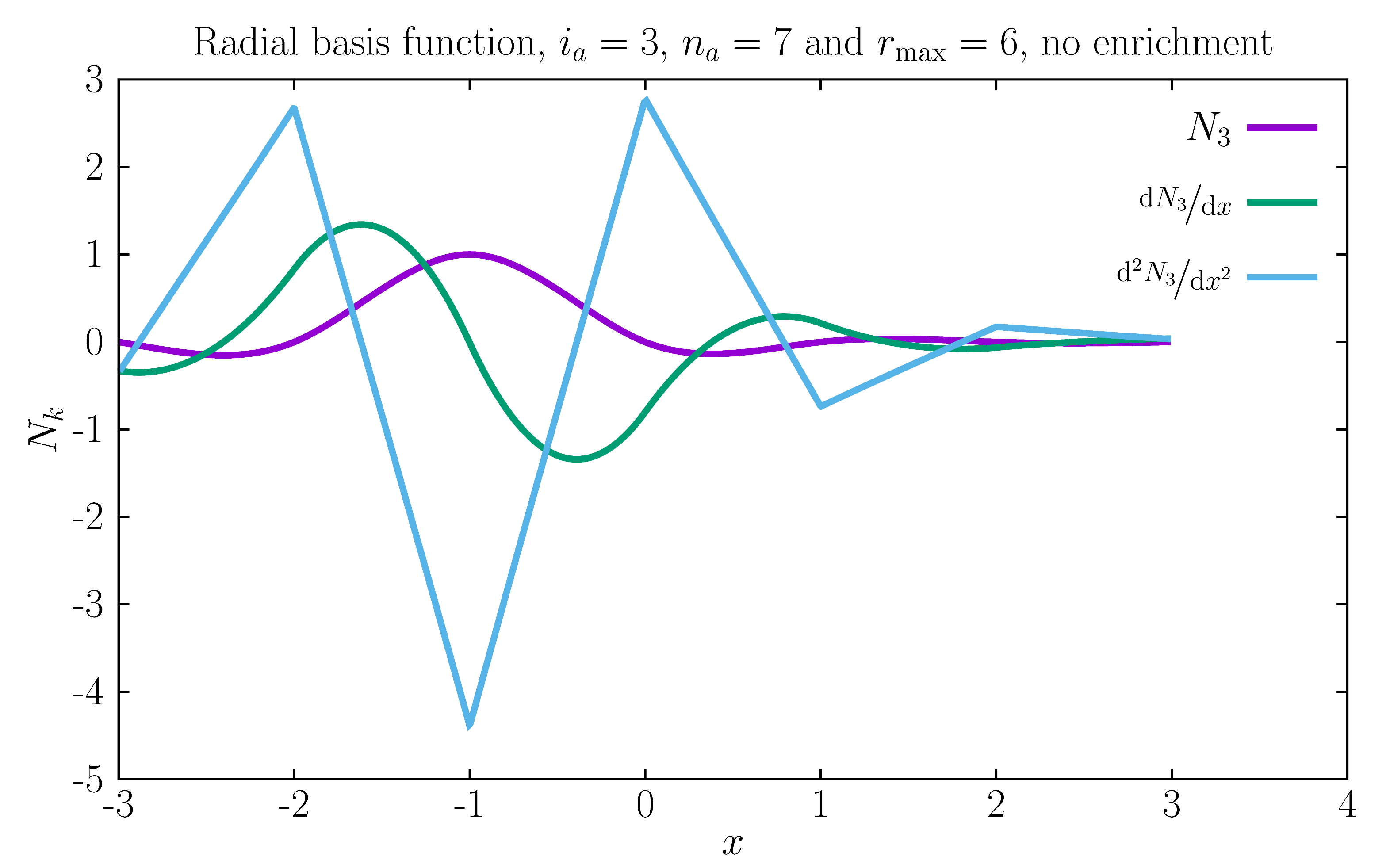
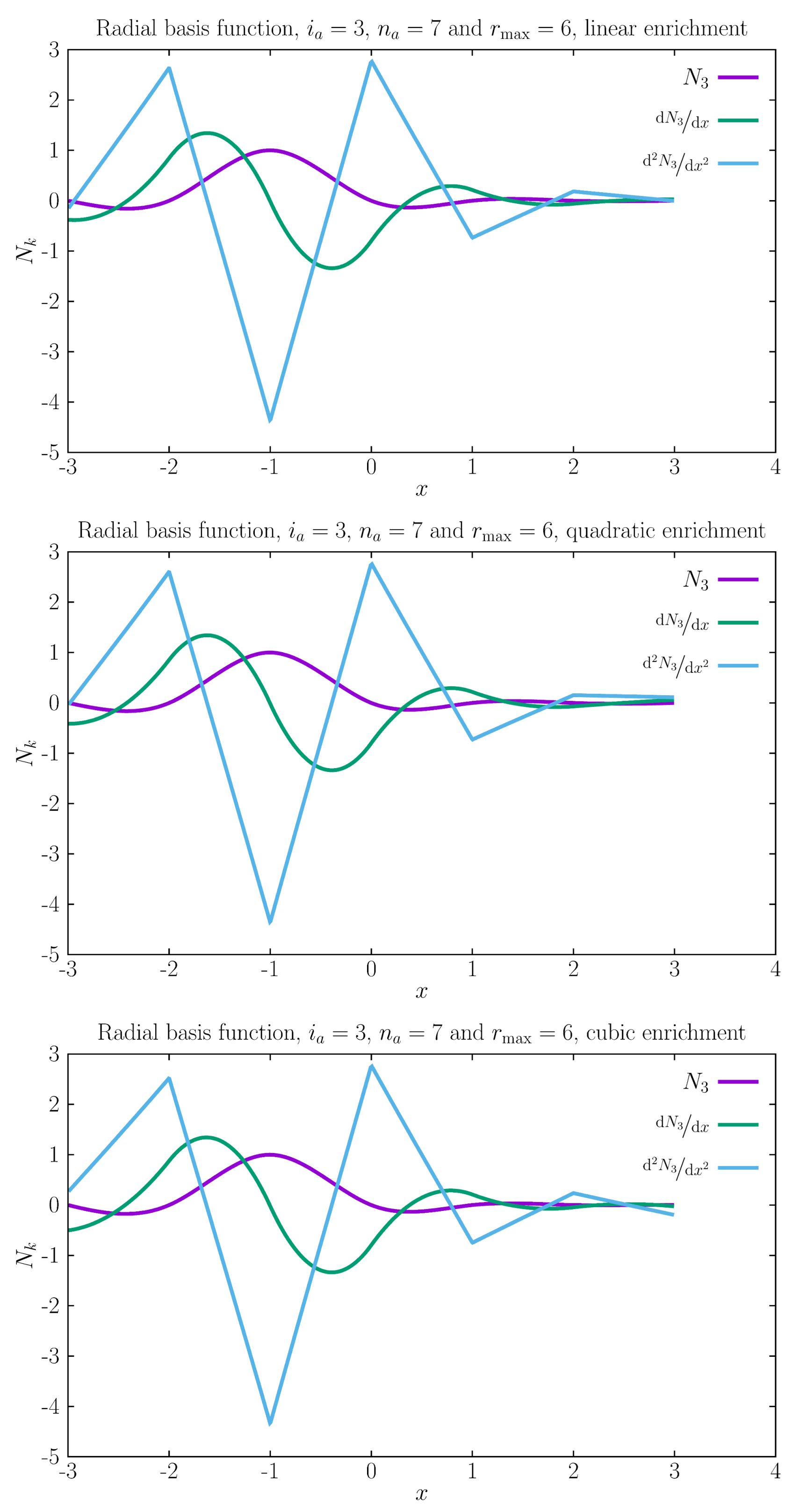
A plot of the shape functions and derivatives is exhibited in Figure 1. We observe that the second derivative is quasilinear, regardless of the polynomial enrichment. The reason for this behavior is that the shape functions depend on the radius and this will appear as a cubic power in the denominator of the derivative with respect to the position $\mathit{X}$. Since a shape function derivative is a sum of two terms, (17), the radial basis term imposes the smoothness of the second derivative. Note that even with polynomial enrichment, the second derivative is continuous. A simple calculation shows that only the fourth derivative is discontinuous.

Figure 1. For nodes $\{-3,-2,-1,0,+1,+2,+3\},$ shape function number 3 and its first and second derivatives.

RBFs are implemented in our own software SimPlas (www.simplassoftware.com), cf. [24], using Mathematica [25] with the AceGen add-on [26]. The specific source code for the RBF part of this work is provided in Github [27].

3. Green–Lagrange Strain, Its Material Derivative and Nodal Sensitivity

Using shape functions and their first and second derivatives obtained from the meshless formalism, the following notation is adopted:

$$\begin{array}{cc}{N}_K\left(\mathit{X}\right)\hfill & \equiv {\left[\mathit{N}\left(\mathit{X}\right)\right]}_K\hfill \end{array}$$

(23)

$$\begin{array}{cc}{N}_{Ki}\left(\mathit{X}\right)\hfill & =\partial N_K\left(\mathit{X}\right)/\partial X_i\hfill \end{array}$$

(24)

$$\begin{array}{cc}{N}_{Kij}\left(\mathit{X}\right)\hfill & ={\partial }^2{N}_K\left(\mathit{X}\right)/\partial X_i\partial X_j\hfill \end{array}$$

(25)

where the upper-case K identifies a node, see, e.g., [28]. Given the nodal spatial coordinates ${\mathit{x}}_L,$ with L being the node number, the deformation gradient and its material derivative are given, respectively, by:

$$\begin{array}{cc}\hfill F_{ij}\left(\mathit{X}\right)& =N_{Lj}\left(\mathit{X}\right)x_{Li}\hfill \end{array}$$

(26)

$$\begin{array}{cc}\hfill F_{ijk}\left(\mathit{X}\right)& =N_{Ljk}\left(\mathit{X}\right)x_{Li}\hfill \end{array}$$

(27)

where the sum is implied in the nodal index L. With respect to the nodal coordinates, the derivatives of the deformation gradients (26) and (27) are calculated as:

$$\begin{array}{cc}\hfill F_{ij,Lm}\left(\mathit{X}\right)& =N_{Lj}\left(\mathit{X}\right){\delta }_{mi}\hfill \end{array}$$

(28)

$$\begin{array}{cc}\hfill F_{ijk,Lm}\left(\mathit{X}\right)& =N_{Ljk}\left(\mathit{X}\right){\delta }_{mi}\hfill \end{array}$$

(29)

where the comma separates the continuum mechanics indices from the nodal quantities. Note that the deformation gradient and its material gradient are linear functions of the nodal coordinates. The Green–Lagrange strain and its first material derivative can be written using index notation as:

$$\begin{array}{cc}\hfill {\left[\mathit{E}\right]}_{ij}& =\frac{1}{2}\left(F_{ni}{F}_{nj}-{\delta }_{ij}\right)\hfill \end{array}$$

(30)

$$\begin{array}{cc}\hfill {\left[\nabla \mathit{E}\right]}_{ijl}& =\frac{1}{2}\left(F_{nil}{F}_{nj}+F_{ni}{F}_{njl}\right)\hfill \end{array}$$

(31)

with an implicit sum on n. Using the same notation, the following identities are a result of the chain rule:

$$\begin{array}{cc}\hfill {\left[\mathit{E}\right]}_{ij,Lm}& =\frac{1}{2}\left(F_{ni,Lm}{F}_{nj}+F_{ni}{F}_{nj,Lm}\right)\hfill \end{array}$$

(32)

$$\begin{array}{cc}\hfill {\left[\mathit{E}\right]}_{ij,Lm,Kl}& =\frac{1}{2}\left(F_{ni,Lm}{F}_{nj,Kl}+F_{ni,Kl}{F}_{nj,Lm}\right)\hfill \end{array}$$

(33)

$$\begin{array}{cc}\hfill {\left[\nabla \mathit{E}\right]}_{ijl,Lm}& =\frac{1}{2}\left(F_{nil,Lm}{F}_{nj}+F_{ni,Lm}{F}_{njl}+F_{nil}{F}_{nj,Lm}+F_{ni}{F}_{njl,Lm}\right)\hfill \end{array}$$

(34)

$$\begin{array}{cc}\hfill {\left[\nabla \mathit{E}\right]}_{ijl,Lm,Kl}& =\frac{1}{2}\left(F_{nil,Lm}{F}_{nj,Kl}+F_{ni,Lm}{F}_{njl,Kl}+F_{nil,Kl}{F}_{nj,Lm}+F_{ni,Kl}{F}_{njl,Lm}\right)\hfill \end{array}$$

(35)

After replacing (28) and (29) in (32)–(35), it is straightforward to obtain:

$$\begin{array}{cc}\hfill {\left[\mathit{E}\right]}_{ij}& =\frac{1}{2}\left(N_{Ki}{N}_{Lj}{x}_{Km}{x}_{Lm}-{\delta }_{ij}\right)\hfill \end{array}$$

(36)

$$\begin{array}{cc}\hfill {\left[\mathit{E}\right]}_{ij,Lm}& =\frac{1}{2}\left(N_{Li}{F}_{mj}+N_{Lj}{F}_{mi}\right)\hfill \end{array}$$

(37)

$$\begin{array}{cc}\hfill {\left[\mathit{E}\right]}_{ij,Lm,Kl}& =\frac{1}{2}\left(N_{Li}{N}_{Kj}+N_{Lj}{N}_{Ki}\right){\delta }_{ml}\hfill \end{array}$$

(38)

$$\begin{array}{cc}\hfill {\left[\nabla \mathit{E}\right]}_{ijn}& =\frac{1}{2}\left(N_{Kin}{N}_{Lj}+N_{Ki}{N}_{Ljn}\right)x_{Km}{x}_{Lm}\hfill \end{array}$$

(39)

$$\begin{array}{cc}\hfill {\left[\nabla \mathit{E}\right]}_{ijn,Lm}& =\frac{1}{2}\left(N_{Lin}{F}_{mj}+N_{Ljn}{F}_{mi}+N_{Lj}{F}_{min}+N_{Li}{F}_{mjn}\right)\hfill \end{array}$$

(40)

$$\begin{array}{cc}\hfill {\left[\nabla \mathit{E}\right]}_{ijn,Lm,Kl}& =\frac{1}{2}\left(N_{Lin}{N}_{Kj}+N_{Ljn}{N}_{Ki}+N_{Lj}{N}_{Kin}+N_{Li}{N}_{Kjn}\right){\delta }_{ml}\hfill \end{array}$$

(41)

Table 1 organizes these quantities by derivative order.

Table 1. Required derivatives of the Green–Lagrange strain, in terms of the shape function derivatives.

	Order of Material Derivative
Nodal Derivative	0	Equation	1	Equation
0	${\left[\mathit{E}\right]}_{ij}$	(36)	${\left[\nabla \mathit{E}\right]}_{ijn}$	(39)
1	${\left[\mathit{E}\right]}_{ij,Lm}$	(37)	${\left[\nabla \mathit{E}\right]}_{ijn,Lm}$	(40)
2	${\left[\mathit{E}\right]}_{ij,Lm,Kl}$	(38)	${\left[\nabla \mathit{E}\right]}_{ijl,Lm,Kl}$	(41)

Introducing the second Piola–Kirchhoff stress $\mathit{S}$, the hyperstress $\Sigma$, which is a third-order tensor, and the corresponding natural conditions [29], we have the following:

• $\mathit{B}$ is the volume force.
• $\mathit{T}$ is the surface loas resulting from the projection of both the second Piola–Kirchhoff and the hyperstress on the undeformed normal $\mathit{N}$, see [16].
• $\tau$ is the double force per unit area. At $\Gamma ,$ the following holds: $\tau -\left[\mathit{N}·\left(\Sigma ·\mathit{N}\right)\right]=0.$
• $\mathit{f}$ is the distributed edge force, which is in action at the locations with discontinuous $\mathit{N}$.

A weak form of equilibrium is established as (see [8]):

$$\underset{\delta W_{\mathrm{int}}}{\underbrace{{\int }_{\Omega }\left(\mathit{S}:\delta \mathit{E}+\Sigma ⋮\delta \nabla \mathit{E}\right)\mathrm{d}V}}=\underset{\delta W_{\mathrm{ext}}}{\underbrace{{\int }_{\Omega }\mathit{B}·\delta \mathbf{u}\mathrm{d}V+{\int }_{\Gamma }\mathit{T}·\delta \mathbf{u}\mathrm{d}\Gamma +{\int }_{\Gamma }\left(\tau \otimes \mathit{N}\right):\delta \nabla \mathbf{u}\mathrm{d}\Gamma +\sum _h{\int }_{{\mathcal{E}}_h}\mathit{F}·\delta \mathbf{u}}}$$

(42)

The Jacobian is obtained by a subsequent variation of (42), which is written as:

$$\mathrm{d}\delta W_{\mathrm{int}}={\int }_{\Omega }\left(\mathrm{d}\mathit{S}:\delta \mathit{E}+\mathit{S}:\mathrm{d}\delta \mathit{E}+\mathrm{d}\Sigma ⋮\delta \nabla \mathit{E}+\Sigma ⋮\mathrm{d}\delta \nabla \mathit{E}\right)\mathrm{d}V$$

(43)

It is not efficient to calculate the quantities of Table 1 separately for the geometric terms. In index notation, the terms are:

$$\begin{array}{cc}\hfill \mathit{S}:\delta \mathit{E}& =\frac{1}{2}{S}_{ij}\left(N_{Li}{F}_{mj}+N_{Lj}{F}_{mi}\right)\delta x_{Lm}\hfill \end{array}$$

(44)

$$\begin{array}{cc}\hfill \Sigma ⋮\delta \nabla \mathit{E}& =\frac{1}{2}{\Sigma }_{ijn}\left(N_{Lin}{F}_{mj}+N_{Ljn}{F}_{mi}+N_{Lj}{F}_{min}+N_{Li}{F}_{mjn}\right)\delta x_{Lm}\hfill \\ \hfill & \mathrm{and}\hfill \end{array}$$

(45)

$$\begin{array}{cc}\hfill \mathit{S}:\mathrm{d}\delta \mathit{E}& =\frac{1}{2}{S}_{ij}\left(N_{Li}{N}_{Kj}+N_{Lj}{N}_{Ki}\right)\delta x_{Lm}\mathrm{d}{x}_{Km}\hfill \end{array}$$

(46)

$$\begin{array}{cc}\hfill \Sigma ⋮\mathrm{d}\delta \nabla \mathit{E}& =\frac{1}{2}{\Sigma }_{ijn}\left(N_{Lin}{N}_{Kj}+N_{Ljn}{N}_{Ki}+N_{Lj}{N}_{Kin}+N_{Li}{N}_{Kjn}\right)\delta x_{Lm}\mathrm{d}{x}_{Km}\hfill \end{array}$$

(47)

4. Constitutive Laws

For the linear case, we adopt the laws established by Dell’Isolla and coworkers [8]. For the second Piola–Kirchhoff stress, Hooke’s law reads:

$$\begin{array}{cc}\hfill S_{ij}& ={\mathcal{C}}_{ijkl}{E}_{kl}\hfill \end{array}$$

with ${\mathcal{C}}_{ijkl}=\lambda {\delta }_{ij}{\delta }_{kl}+\mu \left({\delta }_{ik}{\delta }_{jl}+{\delta }_{il}{\delta }_{jk}\right)$ where $\lambda$ and $\mu$ are the traditional Lamé parameters. These are related to the elastic properties E and $\nu$ as $\mu =\kappa -\frac{2}{3}\mu$ and $\mu =\frac{E}{2\left(1+\nu \right)}$ and $\kappa =\frac{E}{3\left(1-2\nu \right)}$. As in [8], no coupling exists between the Green–Lagrange strain gradient and $\mathit{S}$. A sixth-order tensor is required to relate $\Sigma$ with $\nabla \mathit{E}$:

$$\Sigma =\mathcal{G}⋮\nabla \mathit{E}$$

(48)

For $\Sigma$, only five elastic parameters are required, $c_2$, $c_3$, $c_5,$$c_{11}$ and $c_{15}$:

$$\begin{array}{cc}\hfill {\mathcal{G}}_{ijklpq}=& c_2\left({\delta }_{ij}{\delta }_{kl}{\delta }_{pq}+{\delta }_{ij}{\delta }_{kp}{\delta }_{lq}+{\delta }_{ik}{\delta }_{jq}{\delta }_{lp}+{\delta }_{iq}{\delta }_{jk}{\delta }_{lp}\right)\hfill \\ \hfill +& c_3{\delta }_{ij}{\delta }_{kq}{\delta }_{lp}+c_5\left({\delta }_{ik}{\delta }_{jl}{\delta }_{pq}+{\delta }_{ik}{\delta }_{jp}{\delta }_{lq}+{\delta }_{il}{\delta }_{jk}{\delta }_{pq}+{\delta }_{ip}{\delta }_{jk}{\delta }_{lq}\right)\hfill \\ \hfill +& c_{11}\left({\delta }_{il}{\delta }_{jp}{\delta }_{kq}+{\delta }_{ip}{\delta }_{jl}{\delta }_{kq}\right)+c_{15}\left({\delta }_{il}{\delta }_{jq}{\delta }_{kp}+{\delta }_{ip}{\delta }_{jq}{\delta }_{kl}+{\delta }_{iq}{\delta }_{jl}{\delta }_{kp}+{\delta }_{iq}{\delta }_{jp}{\delta }_{kl}\right)\hfill \end{array}$$

The positive-definiteness of the strain energy corresponding to $\Sigma ⋮\nabla \mathit{E}$, see [8], implies that:

$$\begin{array}{cc}\hfill c_{11}& >0\hfill \\ \hfill -\frac{c_{11}}{2}& <c_{15}<c_{11}\hfill \\ \hfill 5c_3+4c_{11}& >2c_{15}\hfill \\ \hfill c_5& >\frac{c_3\left(3c_{11}+c_{15}\right)+2\left[c_{11}^2-5c_2^2-6c_{15}{c}_2-2c_{15}^2+c_{11}\left(3c_3+c_{15}\right)\right]}{4c_{15}-10c_3-8c_{11}}\hfill \end{array}$$

With these terms, we can rewrite the variation of $\delta W_{\mathrm{int}}$ as:

$$\mathrm{d}\delta W_{\mathrm{int}}={\int }_{\Omega }\left(\left(\mathcal{C}:\mathrm{d}\mathit{E}\right):\delta \mathit{E}+\mathit{S}:\mathrm{d}\delta \mathit{E}+\left(\mathcal{G}⋮\mathrm{d}\nabla \mathit{E}\right)⋮\delta \nabla \mathit{E}+\Sigma ⋮\mathrm{d}\delta \nabla \mathit{E}\right)\mathrm{d}V$$

where $(\mathcal{C}:\mathrm{d}\mathit{E}):\delta \mathit{E}$ is given by:

$$\begin{array}{cc}\hfill \left(\mathcal{C}:\mathrm{d}\mathit{E}\right):\delta \mathit{E}& =\{\lambda {\left(\nabla N_K·\nabla N_L\right)}^2+\mu \left[2N_{K2}{N}_{K3}{N}_{L2}{N}_{L3}\right.\hfill \\ \hfill & +2N_{K1}{N}_{L1}{N}_{K2}{N}_{L2}+2N_{K1}{N}_{L1}{N}_{K3}{N}_{L3}\hfill \\ \hfill & +N_{K1}^2\left(2N_{L1}^2+N_{L2}^2+N_{L3}^2\right)\hfill \\ \hfill & +N_{K2}^2\left(N_{L1}^2+2N_{L2}^2+N_{L3}^2\right)\hfill \\ \hfill & +\left.N_{K3}^2\left(N_{L1}^2+N_{L2}^2+2N_{L3}^2\right)\right]\}\hfill \\ \hfill & ·\left(\delta {\mathit{X}}_L·{\mathit{X}}_K\right)\left(\mathrm{d}{\mathit{X}}_K·{\mathit{X}}_L\right)\hfill \end{array}$$

The term $\left(\mathcal{G}⋮\mathrm{d}\nabla \mathit{E}\right)⋮\delta \nabla \mathit{E}$ is too long to be written here and can be consulted in [27] where the Mathematica/Acegen sheets are stored. A PDF version of this term can be consulted in https://github.com/PedroAreiasIST/RBF/blob/main/mls3dstrainssecondkernel.pdf (accessed on 6 June 2022).

5. Homogenization

For the determination of the seven properties E, $\nu ,$$c_2$, $c_3$, $c_5$, $c_{11}$ and $c_{15}$, a homogenization process based on a multiple-RVE discretization is adopted. If an RVE with volume $V_c$ is considered, where coordinates are identified as ${\mathit{X}}^c$ and displacement as ${\mathit{u}}^c$, we use volume averaging to obtain the first and second macro displacement gradients:

$$\begin{array}{cc}\hfill \frac{\partial u_i}{\partial X_j}& \equiv \frac{1}{V_c}{\int }_{{\Omega }_c}\frac{\partial u_i^c}{\partial X_j^c}\mathrm{d}{V}_c=F_{ij}-{\delta }_{ij}\hfill \\ \hfill \frac{{\partial }^2{u}_i}{\partial X_j\partial X_k}& \equiv \frac{1}{V_c}{\int }_{{\Omega }_c}\frac{\partial u_i^c}{\partial X_j^c\partial X_k^c}\mathrm{d}{V}_c=F_{ijk}\hfill \end{array}$$

(49)

from which $\mathit{E}$ and $\nabla \mathit{E}$ are obtained using (30) and (31).

This is implemented in SimPlas (www.simplassoftware.com) (accessed on 6 June 2022), cf. [24], using Mathematica [25] with the AceGen add-on [26]. The source code for the second derivatives is also provided in [27].

Of course, for a given set of essential boundary conditions, we have

$$\psi \left(\mathit{p}\right)\equiv \frac{1}{2}\mathit{S}:\mathit{E}+\frac{1}{2}\Sigma ⋮\nabla \mathit{E}$$

(50)

where $\mathit{p}=\left\{\mu ,\lambda ,c_2,c_3,c_5,c_{11},c_{15}\right\}$ is the constitutive property array. By equating the RVE energy to $\psi \left(\mathit{p}\right)$, we obtain the following identity:

$$r(\mu ,\lambda ,c_2,c_3,c_5,c_{11},c_{15})=\psi (\mu ,\lambda ,c_2,c_3,c_5,c_{11},c_{15})-\underset{{\psi }_c}{\underbrace{\frac{1}{V_c}{\int }_{{\Omega }_c}\frac{1}{2}{\mathit{S}}^c:{\mathit{E}}^c\mathrm{d}{V}_c}}=0$$

(51)

which is the extended Hill–Mandel condition. Given that the energy of the RVE, ${\psi }_c$, depends on each load case $L=1,\dots ,n_L$, with $n_L>7$, an over-determined system is obtained from identities (51) as:

$$\begin{array}{cc}\hfill {\psi }_1\left(\mu ,\lambda ,c_2,c_3,c_5,c_{11},c_{15}\right)-{\psi }_{c1}& =0\hfill \\ \hfill {\psi }_2\left(\mu ,\lambda ,c_2,c_3,c_5,c_{11},c_{15}\right)-{\psi }_{c2}& =0\hfill \\ \hfill \cdots & \cdots \hfill \\ \hfill {\psi }_{n_L}\left(\mu ,\lambda ,c_2,c_3,c_5,c_{11},c_{15}\right)-{\psi }_{c{n}_L}& =0\hfill \end{array}$$

(52)

The vector form of (52) is written as:

$$\psi \left(\mu ,\lambda ,c_2,c_3,c_5,c_{11},c_{15}\right)-{\psi }_c=\mathbf{0}$$

By using least-squares, we can replace the over-determined system (52) by:

$$\underset{\mu ,\lambda ,c_2,c_3,c_5,c_{11},c_{15}}{min}\frac{1}{2}\left(\psi \left(\mu ,\lambda ,c_2,c_3,c_5,c_{11},c_{15}\right)-{\psi }_c\right)·\left(\psi \left(\mu ,\lambda ,c_2,c_3,c_5,c_{11},c_{15}\right)-{\psi }_c\right)$$

(53)

which can be solved as the linear system:

$$\left[{\left(\partial \psi /\partial \mathit{p}\right)}^T\otimes \left(\partial \psi /\partial \mathit{p}\right)\right]·\mathit{p}={\psi }_c·MM\partial \psi /\partial \mathit{p}$$

(54)

The dependence of the energy vector $\psi$ on $\mathit{p}$ is linear and this is reflected in the left-hand side of (54). The derivative of $\psi (\mu ,\lambda ,c_2,c_3,c_5,c_{11},c_{15})$ with respect to the properties is obtained as follows:

$$\begin{array}{cc}\hfill \frac{\partial \psi (\mu ,\lambda ,c_2,c_3,c_5,c_{11},c_{15})}{\partial \mu }& =E_{11}^2+E_{22}^2+E_{33}^2+2E_{12}^2+2E_{13}^2+2E_{23}^2\hfill \\ \hfill \frac{\partial \psi (\mu ,\lambda ,c_2,c_3,c_5,c_{11},c_{15})}{\partial \lambda }& =\frac{1}{2}{\left(E_{11}+E_{22}+E_{33}\right)}^2\hfill \\ \hfill \frac{\partial \psi (\mu ,\lambda ,c_2,c_3,c_5,c_{11},c_{15})}{\partial c_2}& =2\sum _i\left[\left(\sum _j{E}_{ijj}\right)\left(\sum _j{E}_{jji}\right)\right]\hfill \\ \hfill \frac{\partial \psi (\mu ,\lambda ,c_2,c_3,c_5,c_{11},c_{15})}{\partial c_3}& =\frac{1}{2}\sum _i{\left(\sum _k{E}_{kki}\right)}^2\hfill \\ \hfill \frac{\partial \psi (\mu ,\lambda ,c_2,c_3,c_5,c_{11},c_{15})}{\partial c_5}& =2\sum _i{\left(\sum _j{E}_{ijj}\right)}^2\hfill \\ \hfill \frac{\partial \psi (\mu ,\lambda ,c_2,c_3,c_5,c_{11},c_{15})}{\partial c_{11}}& =2\sum _i\sum _j\sum E_{ijk}^2\hfill \\ \hfill \frac{\partial \psi (\mu ,\lambda ,c_2,c_3,c_5,c_{11},c_{15})}{\partial c_{15}}& =2\left[E_{111}^2+E_{222}^2+E_{333}^2+E_{121}^2+E_{122}^2\right.\hfill \\ \hfill & +\left.E_{231}^2+E_{131}^2+E_{133}^2+E_{232}^2+E_{233}^2\right]\hfill \\ \hfill & +4E_{123}{E}_{231}+4E_{223}{E}_{232}+4E_{133}{E}_{331}\hfill \\ \hfill & +4E_{233}{E}_{332}+4E_{112}{E}_{121}+4E_{131}{E}_{113}+2E_{123}{E}_{132}+2E_{122}{E}_{221}\hfill \end{array}$$

Each load case of the RVE provides a specific energy equivalence relation. Least-squares is adopted for the properties $\mathit{p}={\{\mu ,\lambda ,c_2,c_3,c_5,c_{11},c_{15}\}}^T$. We chose, for each displacement component, the following polynomial basis:

$$\mathit{B}=\left\{X_1^c,X_2^c,X_3^c,X_1^c{X}_2^c,X_2^c{X}_3^c,X_1^c{X}_3^c,X_1^{c2},X_2^{c2},X_3^{c2}\right\}$$

(55)

which produces an over-determined system with $3\times 9$ equations and seven unknowns. For all boundary nodes, we have $i_c=1,\dots ,27$:

$$\begin{array}{cc}\hfill u_{i_d\left(i_c\right)}& =B_{i_t\left(i_c\right)}\hfill \end{array}$$

(56)

$$\begin{array}{cc}\hfill u_{j_d\ne i_d}& =0\hfill \end{array}$$

(57)

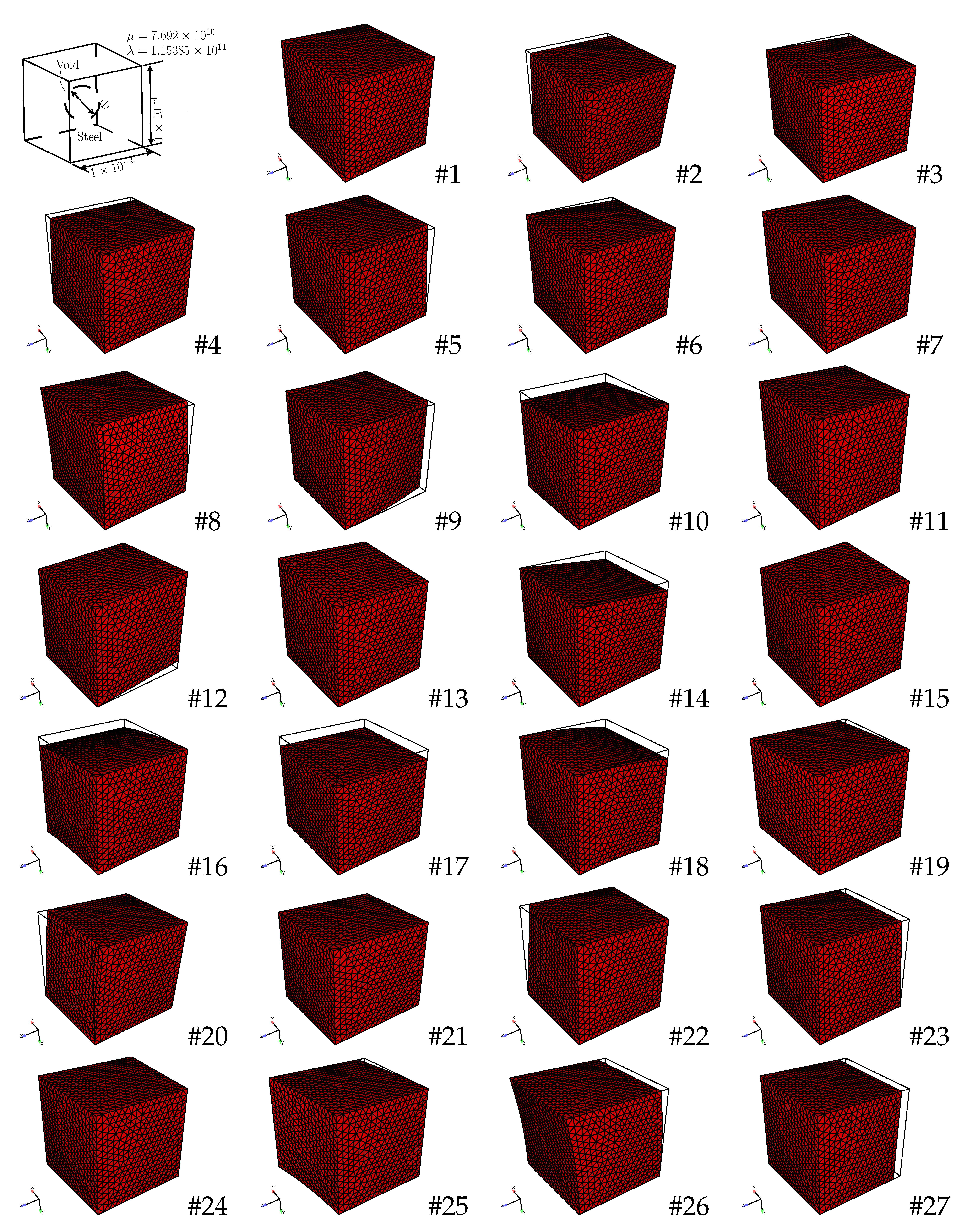
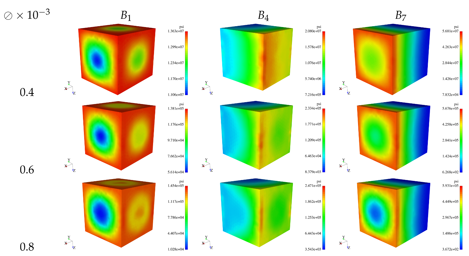
with $i_d=1+\frac{i_c-1}{9}$ and $i_t=1+\mathrm{MOD}\left[i_c-1,9\right]$. Table 2 shows all the imposed displacement cases and the RVE configurations are displayed in Figure 2. In this Figure, ⊘ represents the spherical void diameter. The effect of the spherical voids is clearly shown in Figure 3 for the three void radii.

Table 2. Imposed displacements at the RVE boundaries.

$\mathit{X}\in {\mathbf{\Gamma }}_{\mathit{c}}$
${\mathit{i}}_{\mathit{c}}$	${\mathit{u}}_{\mathbf{1}}\left(\mathit{X}\right)$	${\mathit{u}}_{\mathbf{2}}\left(\mathit{X}\right)$	${\mathit{u}}_{\mathbf{3}}\left(\mathit{X}\right)$	${\mathit{i}}_{\mathit{c}}$	${\mathit{u}}_{\mathbf{1}}\left(\mathit{X}\right)$	${\mathit{u}}_{\mathbf{2}}\left(\mathit{X}\right)$	${\mathit{u}}_{\mathbf{3}}\left(\mathit{X}\right)$	${\mathit{i}}_{\mathit{c}}$	${\mathit{u}}_{\mathbf{1}}\left(\mathit{X}\right)$	${\mathit{u}}_{\mathbf{2}}\left(\mathit{X}\right)$	${\mathit{u}}_{\mathbf{3}}\left(\mathit{X}\right)$
1	$B_1$	0	0	10	0	$B_1$	0	19	0	0	$B_1$
2	$B_2$	0	0	11	0	$B_2$	0	20	0	0	$B_2$
3	$B_3$	0	0	12	0	$B_3$	0	21	0	0	$B_3$
4	$B_4$	0	0	13	0	$B_4$	0	22	0	0	$B_4$
5	$B_5$	0	0	14	0	$B_5$	0	23	0	0	$B_5$
6	$B_6$	0	0	15	0	$B_6$	0	24	0	0	$B_6$
7	$B_7$	0	0	16	0	$B_7$	0	25	0	0	$B_7$
8	$B_8$	0	0	17	0	$B_8$	0	26	0	0	$B_8$
9	$B_9$	0	0	18	0	$B_9$	0	27	0	0	$B_9$

Figure 2. RVE deformed $i_c=1,\cdots ,27$ configurations.

Figure 3. RVE: contour plots for $\psi$ with $B_1$, $B_4$ and $B_7$ for different void diameters ⊘.

We assess a single cell of the RVE, with the characteristic node distances $h=3.75\times {10}^{-5}$, $h=5.00\times {10}^{-5}$, $h=7.5\times {10}^{-5}$ and $h=10.0\times {10}^{-5}$. Table 3 shows the evolution of the constitutive properties for $\oslash =0.4\times {10}^{-3},0.6\times {10}^{-3}$ and $0.8\times {10}^{-3}$.

Table 3. Convergence of properties.

$\oslash =4\times {10}^{-4}$
$h(\times {10}^{-3})$	$\mu \times {10}^9$	$\lambda \times {10}^9$	$c_2\times {10}^9$	$c_3\times {10}^9$	$c_5\times {10}^9$	$c_{11}\times {10}^9$	$c_{15}\times {10}^9$
$0.075$	$73.945$	$111.273$	$-58.693$	$117.387$	$29.346$	$42.555$	$-21.277$
$0.0625$	$73.928$	$110.370$	$-47.625$	$95.250$	$23.812$	$45.283$	$-22.641$
$0.05$	$73.795$	$109.453$	$-45.648$	$91.297$	$22.824$	$45.325$	$-22.662$
$0.0375$	$73.794$	$108.535$	$-39.075$	$78.151$	$19.537$	$47.617$	$-23.808$
0 (extrap.)	$73.602$	$105.800$	$-20.387$	$40.774$	$10.194$	$52.048$	$-26.024$
$\oslash =6\times {10}^{-4}$
$h(\times {10}^{-4})$	$\mu \times {10}^9$	$\lambda \times {10}^9$	$c_2\times {10}^9$	$c_3\times {10}^9$	$c_5\times {10}^9$	$c_{11}\times {10}^9$	$c_{15}\times {10}^9$
$0.075$	$64.866$	$88.444$	$-46.959$	$93.918$	$23.479$	$41.557$	$-20.778$
$0.0625$	$64.609$	$87.515$	$-41.722$	$83.445$	$20.861$	$42.334$	$-21.167$
$0.05$	$64.515$	$87.425$	$-38.058$	$76.116$	$19.029$	$43.695$	$-21.847$
$0.0375$	$64.618$	$87.406$	$-33.496$	$66.992$	$16.748$	$44.645$	$-22.322$
0 (extrap.)	$64.275$	$86.256$	$-20.2349$	$40.4698$	$10.117$	$47.839$	$-23.919$
$\oslash =8\times {10}^{-4}$
$h(\times {10}^{-4})$	$\mu \times {10}^9$	$\lambda \times {10}^9$	$c_2\times {10}^9$	$c_3\times {10}^9$	$c_5\times {10}^9$	$c_{11}\times {10}^9$	$c_{15}\times {10}^9$
$0.075$	$49.960$	$62.568$	$-37.702$	$75.405$	$18.851$	$36.828$	$-18.414$
$0.0625$	$49.487$	$59.008$	$-31.970$	$63.940$	$15.985$	$37.774$	$-18.887$
$0.05$	$49.532$	$59.246$	$-29.966$	$59.933$	$14.983$	$37.995$	$-18.997$
$0.0375$	$49.472$	$59.103$	$-26.620$	$53.240$	$13.310$	$38.702$	$-19.351$
0 (extrap.)	$48.974$	$55.411$	$-15.702$	$31.404$	$7.851$	$40.455$	$-20.227$

A quadratic fit of $\mathit{p}$ with ⊘ will result in:

$$\mathit{p}\left(\oslash \right)=\left\{\begin{array}{c}-74.672{\oslash }^2+28.037\oslash +74.335\\ -114.259{\oslash }^2+43.537\oslash +110.987\\ 54.759{\oslash }^2-53.998\oslash -7.549\\ -109.517{\oslash }^2+107.996\oslash +15.0981\\ -27.3793{\oslash }^2+26.9991\oslash +3.77452\\ -39.7131{\oslash }^2+18.672\oslash +50.9333\\ 19.8565{\oslash }^2-9.33602\oslash -25.4666\end{array}\right\},\oslash \in [0.4,0.8]$$

(58)

For comparison, a classical homogenization procedure for the same problem will result in consistent but slightly distinct results. This is to be expected, as closed-form solutions for the gradient model with the present void problem are not present in the literature. The results from Chakraborty [30] are adapted, with an equivalent void diameter ⊘ corresponding to the reported void fraction, and are shown in Table 4. Since the diameters do not coincide, we use the quadratic fit for the Lamé parameters (58) to calculate our values.

Table 4. Comparison between homogenized Young’s modulus with the gradient model and classical closed-form solution [30].

Void Fraction [30]	Equivalent ⊘	$\mathit{E}/{\mathit{E}}_0$ [30]	Present $\mathit{E}/{\mathit{E}}_0$ (With Interpolation)
$0.065$	$0.498852$	$0.91297$	$0.90633$
$0.110$	$0.594472$	$0.86701$	$0.83963$
$0.180$	$0.700527$	$0.80543$	$0.74484$
$0.270$	$0.801903$	$0.73112$	$0.63378$

6. Macroscopic Size Effect

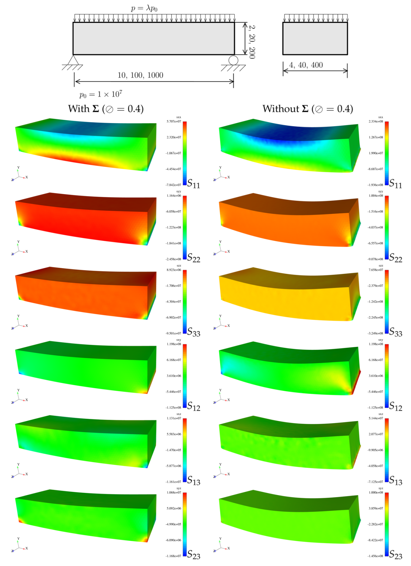
With the fitted properties, we validate the formulation with two exercises: The first one evaluates the effect of specimen size on the load/displacement results and the second shows the objectivity of stress components for a V-notched specimen. The first problem is identified in Figure 4. It is a parallelepiped beam, twice simply supported and under uniform load. A full 3D analysis is performed with edge effects being observed for the classical elasticity model, see Figure 4. This figure shows all six stress components for both models. 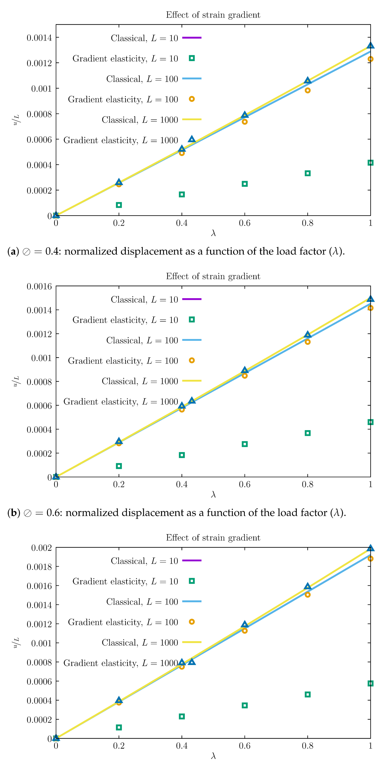Figure 5 presents the results for the size effect for three specimens: $L=10,100$ and 1000 mm. As theoretically predicted, smaller specimens show additional stiffness when the gradient model is considered. In addition, larger values of ⊘ decrease the stiffness of smaller specimens, due to both the reduced elastic modulus and also the effect of the strain gradient. 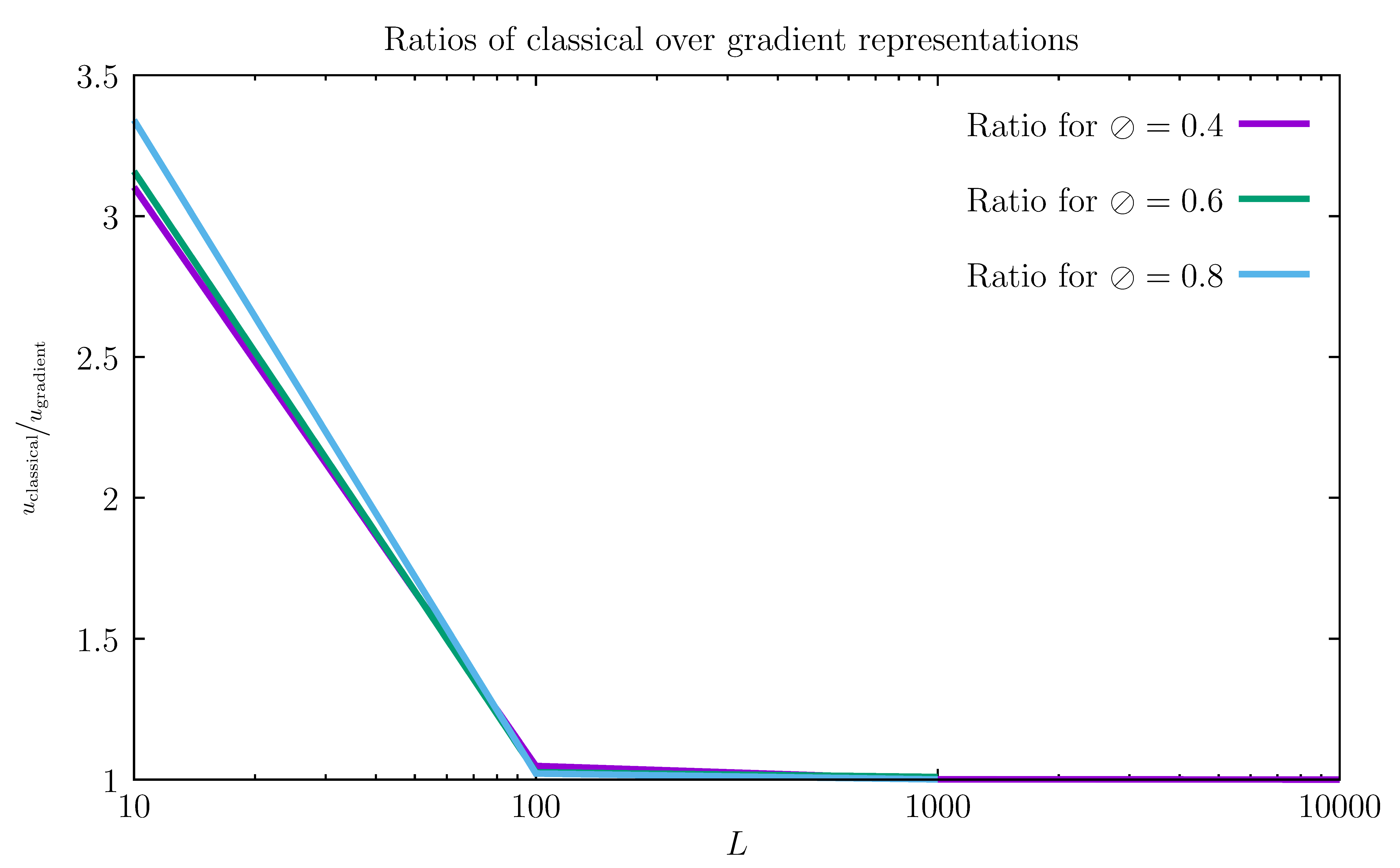Figure 6 shows the effect of L in the ratio between the displacements of the classical elasticity model and the gradient model. The effect is pronounced for the smaller specimen but then dissipates as the void dimensions become much smaller than the overall dimensions of the part.

Figure 4. Simply supported beam under uniform pressure: relevant dimensions and $\mathit{S}$-contour plots for $\oslash =0.4$. Displacement is $10\times$ magnified.

Figure 5. Size effect for $\oslash =0.4,0.6$ and $0.8$ and four beam sizes.

Figure 6. Ratio of results as functions of L.

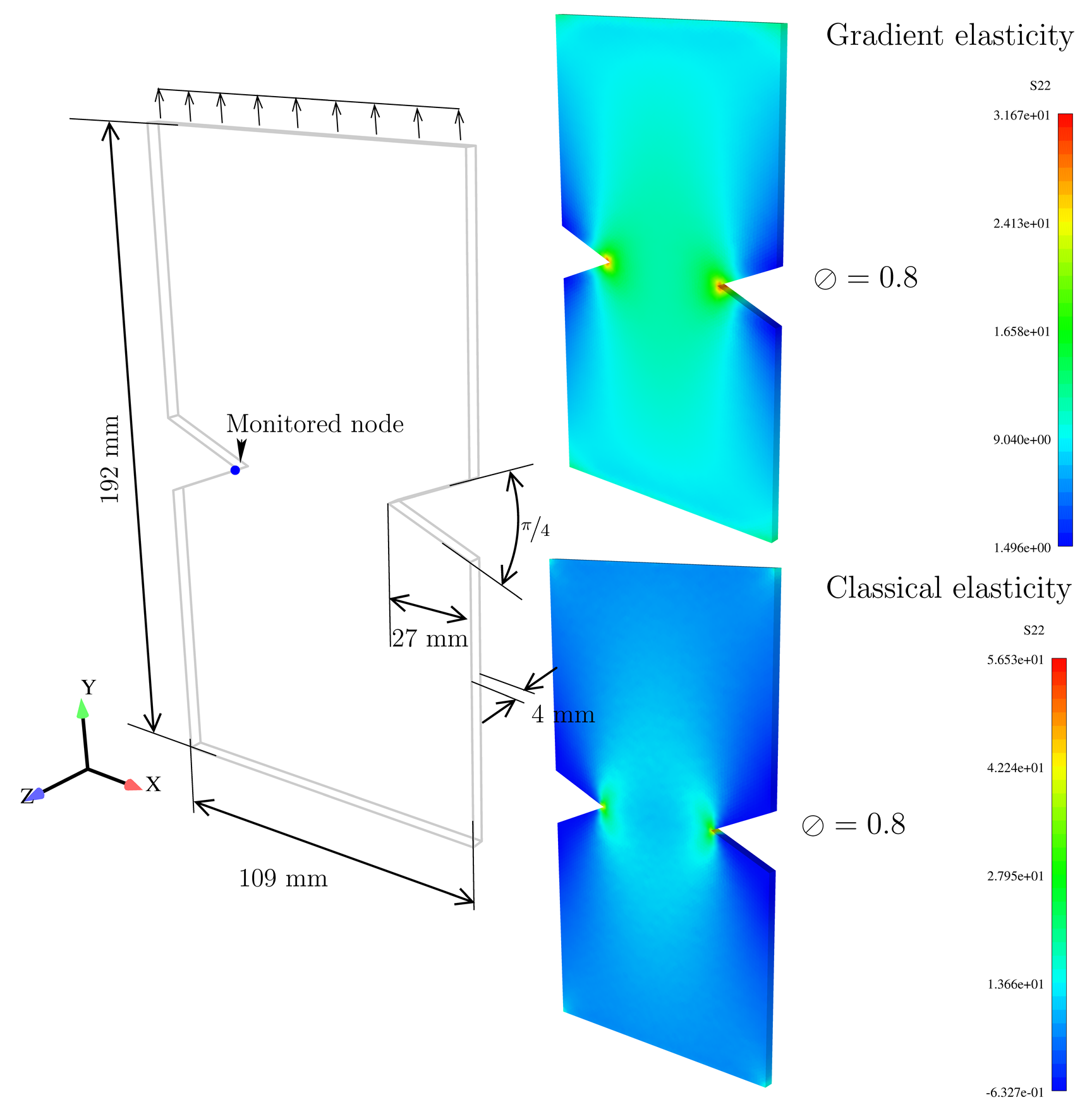
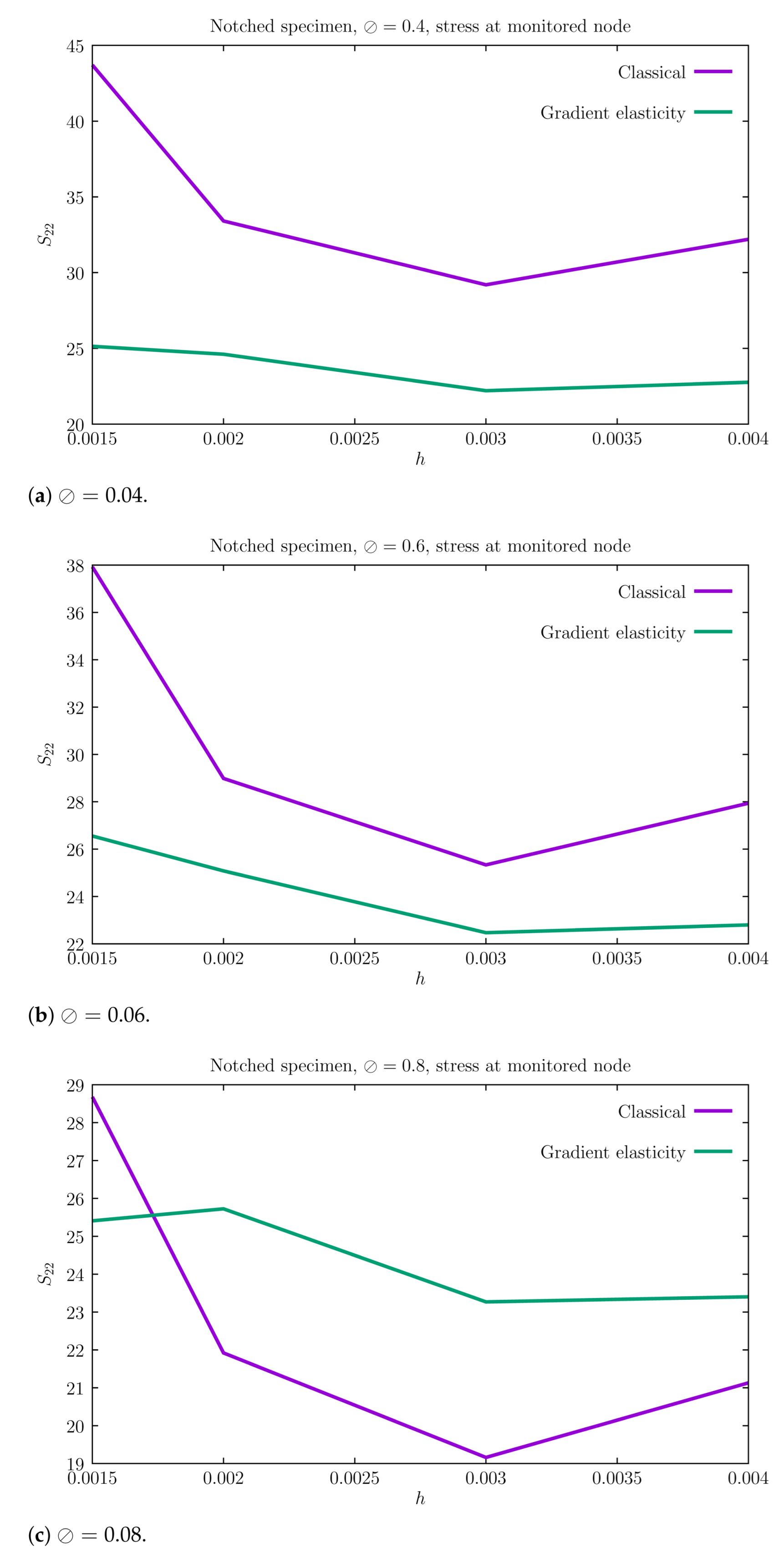
We now consider a notched specimen, as depicted in Figure 7. It consists of a rectangular plate with two sharp notches. In terms of discretization, four point distributions with lengths $h=0.004$, $h=0.003$, $h=0.002$ and $h=0.0015$ are tested. The goal here is to inspect the notch sensitivity when the strain gradient effect is present in the elastic law. It is known that singularities disappear in gradient solutions, and therefore discrete objectivity is to be expected. Contour plots for $S_{22}$ are shown in Figure 7. For the classical elasticity case, a sharper stress concentration appears at the notch and this increases with mesh refinement. Table 5 presents the values of $S_{22}$ at the monitored node for the aforementioned values of h. Table 5 reports the notch tip stress components for the two cases and the corresponding graphical representation is shown in Figure 8. We draw the following conclusions:

Figure 7. Notched specimen: geometry and boundary conditions. Dimensions in mm (properties reported in Table 3 are appropriately scaled).

Table 5. Notched specimen: $S_{22}$ at the monitored node for $\oslash =0.4,$$0.6$ and $0.8$.

Mesh	Classical Elasticity			Gradient Elasticity
	$\oslash =\mathbf{0}.\mathbf{4}$	$\oslash =\mathbf{0}.\mathbf{6}$	$\oslash =\mathbf{0}.\mathbf{8}$	$\oslash =\mathbf{0}.\mathbf{4}$	$\oslash =\mathbf{0}.\mathbf{6}$	$\oslash =\mathbf{0}.\mathbf{8}$
$h=0.004$	$32.20$	$27.94$	$21.13$	$22.76$	$22.80$	$23.40$
$h=0.003$	$29.19$	$25.34$	$19.16$	$22.21$	$22.47$	$23.27$
$h=0.002$	$33.41$	$28.99$	$21.92$	$24.62$	$25.08$	$25.73$
$h=0.0015$	$43.71$	$37.92$	$28.68$	$25.14$	$26.56$	$25.41$

Figure 8. Effect of mesh size h on $S_{22}$ at the monitored node (see Figure 7).

• Stresses converge with point refinement, in contrast with the classical elastic model, which predicts a singularity.
• Lower discrepancies between finer and coarser point distributions are observed.
• A very smooth stress distribution is visible in the contour plot, even at the notch tip.

7. Conclusions

In this work, we introduce a model for finite gradient elasticity, specifically a continuum containing spherical voids, using a two-stage (and two-scale) approach. In the first stage, properties for the gradient model are determined from RVE analysis using a least-squares method. Quadratic displacements are applied to the boundary of the RVE and energy equivalence is established, which results in an unique set of seven elastic properties: two for the fourth-order tensor $\mathcal{C}$ and five for the sixth-order tensor $\mathcal{G}$. In terms of discretization, we adopt a meshless method consisting of radial basis function interpolation with polynomial enrichment and we establish both the first and second derivatives of the shape functions in closed form. Note that an FE mesh is adopted for integration purposes. Detailed expressions for the deformation gradient $\mathit{F}$ and its gradient $\nabla \mathit{F}$ are shown and a consistent linearization is performed to ensure the Newton solution. The source code for this work is available in Github [27]. Validation is performed with two 3D numerical examples: the first one demonstrates the presence of size effect (i.e., the stiffening of smaller specimens) and the second example demonstrates the absence of stress singularity and hence the convergence of the discretization scheme.