An Improved Arithmetic Optimization Algorithm and Its Application to Determine the Parameters of Support Vector Machine

Abstract

The arithmetic optimization algorithm (AOA) is a new metaheuristic algorithm inspired by arithmetic operators (addition, subtraction, multiplication, and division) to solve arithmetic problems. The algorithm is characterized by simple principles, fewer parameter settings, and easy implementation, and has been widely used in many fields. However, similar to other meta-heuristic algorithms, AOA suffers from shortcomings, such as slow convergence speed and an easy ability to fall into local optimum. To address the shortcomings of AOA, an improved arithmetic optimization algorithm (IAOA) is proposed. First, dynamic inertia weights are used to improve the algorithm’s exploration and exploitation ability and speed up the algorithm’s convergence speed; second, dynamic mutation probability coefficients and the triangular mutation strategy are introduced to improve the algorithm’s ability to avoid local optimum. In order to verify the effectiveness and practicality of the algorithm in this paper, six benchmark test functions are selected for the optimization search test verification to verify the optimization search ability of IAOA; then, IAOA is used for the parameter optimization of support vector machines to verify the practical ability of IAOA. The experimental results show that IAOA has a strong global search capability, and the optimization-seeking capability is significantly improved, and it shows excellent performance in support vector machine parameter optimization.

1. Introduction

With the prosperous development of science and technology and the economy, intelligence has gradually stepped into many fields, such as science, engineering, the economy, and national defense. Accordingly, numerous complex problems requiring optimization solutions have emerged in these fields. Traditional optimization methods include linear programming, dynamic programming, integer programming, branch-and-bound, and other classical algorithms, which often have poor optimization results and difficulties in meeting practical needs when solving problems with large variable dimensions, high order, many objective functions, and complex constraints. The proposed metaheuristic algorithm provides a new way of thinking for solving various complex and tricky engineering optimization problems. It is investigated that metaheuristic algorithms solve optimization problems with sufficient efficiency and reasonable computational cost compared with exact algorithms [1].

A metaheuristic algorithm is a deterministic algorithm plus heuristic random search to obtain the close-enough solution to the optimization problem through iterative iterations, which includes the following four main categories: Evolutionary Algorithms (EA), Swarm Intelligence Algorithms (SI), Physical Law Based Algorithms (PHA), and Human-Based Algorithms. EA simulates the processes of biological survival and reproduction in nature and the process of continuous evolution through heredity, mutation, and natural selection. Its classical algorithms include the Genetic Algorithm (GE) [2], Differential Evolution (DE) [3], Estimation Of Distribution Algorithms (EDA) [4], DNA Computing [5], Gene Expression Programming (GEP) [6], Memetic Algorithm (MA) [7], and Cultural Algorithms (CA) [8]. SI simulates the hunting strategy and reproductive behavior of natural animal groups, etc., and its classical algorithms include Artificial Bee Colony (ABC) [9], Gray Wolf Optimization (GWO) [10], Particle Swarm Optimization (PSO) [11], Cuckoo Search (CS) [12], Harris Hawks Optimization (HHO) [13], Whale Optimization Algorithm (WOA) [14], Slime Mould Algorithm (SMA) [15], and Seagull Optimization Algorithm (SOA) [16]. PhA is inspired by the laws of physics, and its typical algorithms include Henry Gas Solubility Optimization (HGSO) [17], Big Bang–Big Crunch (BBBC) [18], Multi-verse Optimizer (MVO) [19], Electromagnetic Field Optimization (EFO) [20], and Gravitational Search Algorithm (GSA) [21]. Human-based algorithms inspired by human behavior, typical algorithms include Teaching-Based Learning Algorithms (TBLA) [22], Harmony Search (HS) [23], Imperialist Competitive Algorithm (ICA) [24], Fireworks Algorithm (FWA) [25], and Collective Decision Optimization (CSO) [26]. Meta-heuristic algorithms have the advantages of simple principles, fewer parameter settings, and easy implementation, which have obvious advantages in solving complex optimization problems [27]. Therefore, these algorithms have received extensive attention and research since they were proposed and have been applied to multi-robot cooperation [28], wireless sensor networks [29], object detection [30], honeycomb core design [31], feature selection [32], and multi-objective problems [33].

The arithmetic optimization algorithm (AOA) [34] is a new population-based metaheuristic algorithm proposed by Abualigah et al. The arithmetic optimization algorithm is inspired by the application of arithmetic operators (addition, subtraction, multiplication, and division) in solving arithmetic problems. The algorithm is able to solve optimization problems without computing their derivatives, so applications in other disciplines would be a valuable contribution. For example, Khatir et al. [35] used AOA for damage detection, localization, and quantification of functional gradient material (FGM) plate structures. Deepa et al. [36] used AOA for Alzheimer’s disease (AD) classification. Almalawi et al. [37] used AOA to predict the particle size distribution of heavy metals in the air. Ahmadi et al. [38] used AOA for multiple types of distributed generation (DGs) and energy storage systems (ESSs) for optimal layout. Bhat et al. [39] used AOA for wireless sensor network (WSN) deployment. Similar to numerous other metaheuristics, AOA suffers from shortcomings, such as slow convergence and the tendency to fall into local optimality. Therefore, numerous scholars have made numerous improvements as well as applications of this algorithm. For example, Kaveh et al. [40] modified the original formulation of AOA to enhance exploration and exploitation and applied it to skeleton structure optimization for discrete design variables. Agushaka et al. [41] used natural logarithm and exponential operators to enhance the exploration capability of AOA and applied it to welded beam design (WBD), compression spring design (CSD), and pressure vessel design (PVD). Premkumar et al. [42] proposed a multi-objective arithmetic optimization algorithm formulated and developed based on the mechanisms of elite non-dominance ranking and congestion distance and used it to solve real-world constrained multi-objective optimization problems (RWMOPs). Zheng et al. [43] mixed the viscous and arithmetic optimization algorithms to improve the optimization speed and accuracy of the algorithm and applied it to classical engineering design problems. Abualigah et al. [44] used a differential evolution technique to enhance the local study of AOA and applied it to image segmentation. Ibrahimd et al. [45] proposed an algorithm based on a hybrid of an electrofishing optimization algorithm and an arithmetic optimization algorithm to improve the convergence speed of the algorithm and increase the ability of the algorithm to handle high-dimensional problems and applied it to feature selection. Wang et al. [46] proposed a novel parallel communication strategy for adaptive parallel arithmetic optimization algorithms to prevent the algorithm from falling into local optimal solutions and used it for robot path planning. Ewees et al. [47] mixed arithmetic optimization algorithms with genetic algorithms to enhance their search strategies and adjust the balance of their search strategies directly and used them for feature selection. Abualigah et al. [48] combined the marine predator algorithm and a new integrated variational strategy to improve the convergence speed of the algorithm and apply it to engineering design cases. Khodadadi et al. [49] proposed a dynamically tuned exploration and developed an arithmetic optimization algorithm for a better search phase and applied it to classical engineering problems. Mahajan et al. [50] proposed a hybrid algorithm based on the Aquila optimizer and an arithmetic optimization algorithm to enhance AOA in solving high-dimensional problems. Li et al. [51] introduced a chaotic mapping strategy into the optimization process of AOA to improve its convergence speed and accuracy and applied it to engineering optimization problems. Abd et al. [52] proposed an energy-aware model to enhance the arithmetic optimization algorithm to improve the search capability of the algorithm and used it for the job scheduling problem of fog computing.

Support vector machines (SVMs) were originally proposed by Vapnik et al. [53]. As a machine learning algorithm based on statistical learning theory, SVMs have shown many unique advantages in solving small-sample, nonlinear, and high-dimensional pattern recognition problems and have been successfully applied to pattern recognition [54], medical applications [55], and photovoltaic power generation prediction [56], among other fields. Although SVMs have many advantages in practice, the selection of their internal parameters has a certain degree of influence on the classification performance and the fitting effect of SVM models, and these parameters will negatively affect the generalization performance of SVMs if they are not selected appropriately. Therefore, it is a challenge to select the best model for SVM and find the appropriate internal parameters. Therefore, the proposed algorithm is used for the selection of internal parameters of support vector machines to verify the practical performance of IAOA.

Although AOA has been applied to many aspects, in terms of the algorithm itself, one of the reasons why AOA is prone to local optima and slow convergence during the search process is that the updates of individuals in AOA are only searched around a single global best position. According to Jamil et al. [57], this makes the search strategy highly selective, and other individuals relying on this single centrally guided position update may not be guaranteed to converge to the global best position. Therefore, in this paper, dynamic inertia weights are used to enhance the convergence speed of AOA, and dynamic probability coefficients and triangular mutation strategies are used to enhance the ability of AOA to jump out of the local optimum. The experimental results show that the proposed algorithm’s convergence accuracy, convergence speed, and stability are significantly improved, and IAOA has excellent classification accuracy in the optimization of support vector machine parameters.

The main structure of this paper is as follows: in Section 2, the basic AOA algorithm is introduced; Section 3 introduces the IAOA algorithm; Section 4 presents the results, comparison, and analysis of the experiments; Section 5 presents the application of IAOA in support vector machine parameter optimization; and Section 6 concludes the work and presents future research directions.

2. Basic AOA

The basic AOA utilizes multiplication and division operators for global exploration and addition and subtraction operators for local exploitation.

2.1. Math Optimizer Accelerated (MOA) Function

AOA selects the search phase (whether to execute global exploration or local exploitation) by MOA. A random number r₁ (a random number between 0 and 1) is selected, and if r₁ > MOA(t), then global exploration is executed; otherwise, local exploitation is executed. The mathematical model of MOA is shown in Equation (1):

$$MOA(t)=Min+t\times (\frac{Max-Min}{T})$$

(1)

where t is the current number of iterations, T is the maximum number of iterations, and Max and Min are the maximum and minimum values of the mathematical optimizer acceleration function, respectively.

2.2. Global Exploration

In this stage, AOA mainly uses two search strategies (division search strategy and multiplication search strategy) to find a better candidate solution. A random number r₂ is drawn from [0, 1], and if r₂ < 0.5, the division strategy is executed; otherwise, the multiplication strategy is executed. The mathematical expression of the search is shown in Equation (2):

$$x(t+1)=\{\begin{array}{cc}best(x)÷(MOP(t)+\epsilon )\times L,\hfill & \hfill r_2<0.5\\ best(x)\times MOP(t)\times L,\hfill & \hfill otherwise\end{array}$$

(2)

$$MOP(t)=1-t^{1/\alpha }/T^{1/\alpha }$$

(3)

$$L=(UB-LB)\times \mu +LB$$

(4)

where x(t + 1) denotes the position of t + 1 iterations, best(x) denotes the position of the best individual among the current candidate solutions, ε is a small integer preventing the denominator from being 0, UB and LB denote the upper and lower bounds of the search space, respectively, μ is the control parameter for adjusting the search process, MOP(t) is the mathematical optimization rate coefficient, and α denotes the sensitivity parameter for iterative development accuracy.

2.3. Local Exploitation

In this stage, AOA mainly uses subtractive search strategy and additive search strategy for exploitation calculation. If r₃ < 0.5 (r₃ is a random number between 0 and 1) the subtractive search strategy is used; otherwise, the additive search strategy is used. Its search mathematical expression is shown in Equation (5):

$$x(t+1)=\{\begin{array}{cc}best(x)-MOP(t)\times L,\hfill & \hfill r_3<0.5\\ best(x)+MOP(t)\times L,\hfill & \hfill otherwise\end{array}$$

(5)

The pseudo code of AOA is shown below.

3. Our Proposed IAOA

3.1. Dynamic Inertia Weights

Inertia weights were originally proposed by Shi and Eberhart, and larger inertia weights are beneficial for global exploration and smaller inertia weights are beneficial for local exploitation [58]. Therefore, in this paper, an inertia weight that decreases nonlinearly and exponentially with the number of iterations is introduced, and inertia weights with dynamic coefficients are introduced to improve the search efficiency of the AOA Algorithm 1, which in turn speeds up the convergence of the algorithm. The introduction of dynamic coefficients can improve the flexibility of the inertia weights, and then in the application of the improved algorithm can be perturbed to improve the flexibility of the optimal individual, so as to reduce to a certain extent the degree of the algorithm into the local optimum due to the location update method guided only around the current optimal individual. The dynamic inertia weights are shown in Equation (6):

$$w(t)=c\ast w_{begin}{(\frac{w_{begin}}{w_{end}})}^{1/(1+t/T)}$$

(6)

where the maximum and minimum values of w_begin and w_end inertia weights, c are random values that vary dynamically around value 1. Where the sum of dynamic inertia weights is introduced to Equations (2) and (5), its updated formula becomes Equations (7) and (8):

$$x(t+1)=\{\begin{array}{cc}w(t)\ast best(x)÷(MOP(t)+\epsilon )\times L,\hfill & \hfill r_2<0.5\\ w(t)\ast best(x)\times MOP(t)\times L,\hfill & \hfill otherwise\end{array}$$

(7)

$$x(t+1)=\{\begin{array}{cc}w(t)\ast best(x)-MOP(t)\times L,\hfill & \hfill r_3<0.5\\ w(t)\ast best(x)+MOP(t)\times L,\hfill & \hfill otherwise\end{array}$$

(8)

Algorithm 1: AOA

1.Set population size N, the maximum number of iterations T. 2.Set up the initial parameters t = 0, α, μ. 3.Initialize the positions of the individuals xi (i = 1, 2, …, N). 4.While (t < T) 5.  Update the MOA using Equation (1) and the MOP using Equation (3). 6.  Calculate the fitness values and Determine the best solution. 7.  For i = 1, 2, …, N do 8.    For j = 1, 2, …, Dim 9.      Generate the random values between [0, 1] (r1, r2, r3). 10.      If r1 > MOA 11.        Update the position of x(t + 1) using Equation (2). 12.      Else 13.        Update the position of x(t + 1) using Equation (5) 14.      End if 15.    End for 16.  End for 17.  t = t + 1. 18.End while 19.Return the best solution (x)

3.2. Dynamic Coefficient of Mutation and Triangular Mutation Strategy

Referring to the “mutation” operation in the genetic algorithm, this paper uses a dynamic mutation probability coefficient that increases with the number of iterations so that individuals have a certain chance to enter other search spaces for searching, thus effectively expanding the search range and enhancing the ability of the algorithm to jump out of the local optimum. The dynamic mutation probability coefficient is shown in Equation (9). The triangular mutation strategy [59] makes full use of the information of individuals in the population, so that the information of individuals crosses each other, thus enhancing the diversity of the population and preventing the algorithm from falling into a local optimum in the search process. One of the triangular mutation formulas is shown in Equation (10):

$$p=0.2+0.5\ast t/T$$

(9)

$$\begin{array}{l}X(t)=(X_{r1}+X_{r2}+X_{r3})/3+(t_2-t_1)\ast (X_{r1}-X_{r2})+\\ (t_3-t_2)\ast (X_{r2}-X_{r3})+(t_1-t_3)\ast (X_{r3}-X_{r1})\end{array}$$

(10)

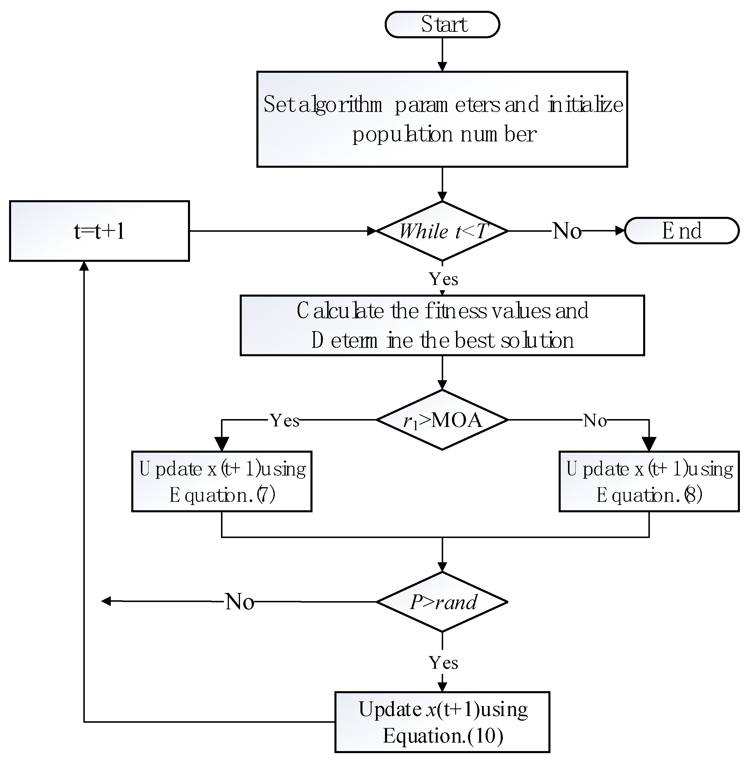
where p denotes the mutation probability coefficient, which gradually increases with the number of iterations, and in the late stage of the algorithm, individuals in the population have a greater probability of entering other spatial searches, which in turn reduces the probability of the algorithm falling into a local optimum. X_r1, X_r2, and X_r3 denote the three randomly selected individuals, (t₂ − t₁), (t₃ − t₂), and (t₁ − t₃) denote the weights of the perturbed part. The triangular mutation strategy is similar to the cross mutation of a genetic algorithm, which makes the information of random individuals cross-fused with each other. This strategy is helpful to prevent the update of individuals only around a single local best position, thus enhancing the algorithm’s ability to jump out of local minima. The pseudo-code and flowchart of IAOA are shown in Algorithm 2 and Figure 1.

Algorithm 2: IAOA

1.Set population size N, the maximum number of iterations T. 2.Set up the initial parameters t = 0, α, μ. 3.Initialize the positions of the individuals xi (i = 1, 2, …, N). 4.While (t < T) 5.  Update the w(t) using Equation (6) 6.  Update the MOA using Equation (1) and the MOP using Equation (3). 7.  Calculate the fitness values and Determine the best solution. 8.  For i = 1, 2, …, N do 9.    For j = 1, 2, …, Dim 10.      Generate the random values between [0, 1] (r1, r2, r3). 11.      If r1 > MOA 12.        Update the position of x(t + 1) using Equation (7). 13.      Else 14.        Update the position of x(t + 1) using Equation (8) 15.      End if 16.    Calculate the p using Equation (9) 17.    if p > rand 18.    Update the position of x(t + 1) using Equation (10). 19.    end if 20.    End for 21.  End for 22.  t = t + 1. 23.End while 24.Return the best solution(x)

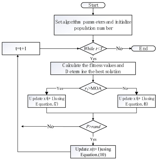
Figure 1. IAOA flow chart.

4. Benchmark Test Function Numerical Experiments and Results

4.1. Experimental Conditions

The environment configuration for this experimental simulation is: 64-bit Win10 operating system; Intel (R) Core (TM) i7-1065G7 CPU with 1.30 GHz; 16 G memory; and the simulation software is MatlabR2019b. This experiment selects six benchmark test functions for experimental test comparison, among which the algorithms compared in this experiment are GA [2], GWO [10], PSO [11], HHO [13], WOA [14], SOA [16], and AOA [34]. For all the tested functions, the population size of the algorithm is 30 and the number of iterations is 500.

4.2. Benchmark Test Functions and Algorithm Parameters

In this experiment, the six benchmark test functions selected are shown in Table 1. Among them, f₁ − f₃ are single-mode test functions, and f₄ − f₆ are multimode test functions. Table 2 shows the parameter settings of all the comparison algorithms.

Table 1. Benchmark test functions.

Formula	Dim	Range	Fmin
$f_1(x)={\displaystyle \sum _{i=1}^n{x}_i^2}$	30/100/200	[−100, 100]	0
$f_2(x)=\max (|x_i|,1\le i\le n)$	30/100/200	[−100, 100]	0
$f_3(x)={\displaystyle \sum _{i=1}^n{(\lfloor x_i+0.5\rfloor )}^2}$	30/100/200	[−100, 100]	0
$f_4(x)=\frac{1}{4000}{\displaystyle \sum _{i=1}^n{x}_i^2-{\displaystyle {\prod }_{i=1}^n\cos (\frac{x_i}{\sqrt{i}})+1}}$	30/100/200	[−600, 600]	0
$\begin{array}{l}{f}_5(x)=\frac{\pi }{n}\{10\sin (\pi y_1)+{\displaystyle \sum _{i=1}^{n-1}{(y_1-1)}^2[1+10{\sin }^2(\pi y_{i+1})]+{(y_n-1)}^2}\}\\ +{\displaystyle \sum _{i=1}^{n}u(x_i,10,100,4)}\\ {\mathrm{y}}_i=1+\frac{x_i+1}{4},u(x_i,a,k,m)=\{\begin{array}{cc}k{(x_i-m)}^m,\hfill & \hfill x_i>a\\ -a,\hfill & \hfill x_i<a\\ k{(-x_i-m)}^m,\hfill & \hfill x_i<-a\end{array}\end{array}$	30/100/200	[−50, 50]	0
$\begin{array}{l}{f}_6(x)=0.1\{{\sin }^2(3\pi x_i){\displaystyle \sum _{i=1}^n{(x_i-1)}^2[1+{\sin }^2(3\pi x_i+1)]+{(x_n-1)}^2[1+{\sin }^2(2\pi x_n)]}\}\\ +{\displaystyle \sum _{i=1}^{n}u(x_i,5,100,4)}\end{array}$	30/100/200	[−50, 50]	0

Table 2. Algorithm parameter settings.

Algorithm	Parameter Setting
GA	Pm = 0.2, Pc = 0.6
GWO	a linearly decreased from 2 to 0
PSO	ω linearly decreased from 0.9 to 0.4, c1 = 2, c2 = 2
HHO	q ∈ [0, 1]; r ∈ [0, 1]; E0 ∈ [−1, 1]; E1 ∈ [0, 2]; E ∈ [−2,2]
WOA	a linearly decreased from 2 to 0, r1 ∈ [0, 1], r2 ∈ [0, 1]
SOA	r1 ∈ [0, 1], r2 ∈ [0, 1]
AOA	r1 ∈ [0, 1], r2 ∈ [0, 1], r3 ∈ [0, 1], u = 0.5, α = 5
IAOA	wbegin = 0.9, wend = 0.4, c ∈ [0.95, 1.05]

4.3. Comparison and Analysis of Experimental Results

To evaluate the performance of the proposed IAOA, numerical experimental simulation tests are performed for all compared algorithms. To avoid the effect of randomness on the test results, each algorithm was run 30 times independently for each test function (Dim = 30), and the mean value of each algorithm with standard deviation was recorded. These data indicators generally reflect the strength of the algorithm’s optimization capability. The mean value reflects the optimization accuracy of the algorithm, and the standard deviation reflects the stability performance of the algorithm. The average running time of each algorithm for each test function is also recorded, which reflects the running complexity of the algorithm. Table 3 provides the test data of all eight algorithms. To evaluate the high-dimensional performance of IAOA, all comparison algorithms are tested in 100 and 200 dimensions, and the test conditions are the same as in 30 dimensions. Only the dimensionality of the test function is changed, and the mean value and standard deviation of the test are recorded. Table 4 records the test data of all algorithms in high-dimensional conditions.

Table 3. Test data.

Function	Indext	Algorithms
		GA	GWO	PSO	HHO	WOA	SOA	AOA	IAOA
f1 (Dim = 30)	Mean	3.17 × 10−5	1.89 × 10−27	3.27 × 10−155	5.52 × 10−94	1.06 × 10−74	5.09 × 10−12	2.58 × 10−10	0.00 × 10+0
	Std	7.39 × 10−5	3.54 × 10−27	1.79 × 10−154	3.01 × 10−93	3.19 × 10−74	7.42 × 10−12	1.41 × 10−9	0.00 × 10+0
	Time	0.1851 s	0.3617 s	0.1343 s	0.1972 s	0.1514 s	0.2589 s	0.1919 s	0.2003 s
f2 (Dim = 30)	Mean	2.42 × 10−3	8.91 × 10−7	3.01 × 10−87	1.03 × 10−49	5.13 × 10+1	5.62 × 10−3	2.85 × 10−2	0.00 × 10+0
	Std	3.20 × 10−3	5.89 × 10−7	1.65 × 10−86	3.51 × 10−49	2.89 × 10+1	1.24 × 10−2	1.86 × 10−2	0.00 × 10+0
	Time	0.0767 s	0.3224 s	0.1521 s	0.2533 s	0.1474 s	0.2557 s	0.2063 s	0.2110 s
f3 (Dim = 30)	Mean	1.36 × 10−5	8.15 × 10−1	1.37 × 10+0	2.14 × 10−4	3.22 × 10−1	3.22 × 10+0	3.14 × 10+0	0.00 × 10+0
	Std	2.50 × 10−5	3.99 × 10−1	2.85 × 10−1	2.93 × 10−4	1.82 × 10−1	5.18 × 10−1	2.40 × 10−1	0.00 × 10+0
	Time	0.0802 s	0.3300 s	0.1386 s	0.3144 s	0.1218 s	0.2586 s	0.1777 s	0.1981 s
f4 (Dim = 30)	Mean	1.66 × 10−4	2.22 × 10−3	1.78 × 10−2	0.00 × 10+0	3.23 × 10−3	2.24 × 10−2	1.67 × 10−1	0.00 × 10+0
	Std	2.76 × 10−4	5.94 × 10−3	6.37 × 10−2	0.00 × 10+0	1.77 × 10−2	2.88 × 10−2	1.41 × 10−1	0.00 × 10+0
	Time	0.0972 s	0.1931 s	0.1013 s	0.2854 s	0.1209 s	0.1533 s	0.1472 s	0.1831 s
f5 (Dim = 30)	Mean	1.22 × 10−4	1.11 × 10−1	2.38 × 10−1	4.04 × 10−6	3.26 × 10−2	4.97 × 10−1	7.30 × 10−1	9.42 × 10−33
	Std	2.40 × 10−4	6.52 × 10−2	3.82 × 10−2	6.63 × 10−6	2.31 × 10−2	1.14 × 10−1	3.37 × 10−2	2.78 × 10−48
	Time	0.1999 s	0.4851 s	0.3792 s	0.9107 s	0.3688 s	0.4361 s	0.4050 s	0.6291 s
f6 (Dim = 30)	Mean	5.13 × 10−5	6.20 × 10−1	1.02 × 10+0	6.12 × 10−5	5.94 × 10−1	2.08 × 10+0	2.83 10+0	1.35 × 10−32
	Std	1.00 × 10−4	2.39 × 10−1	2.05 × 10−1	8.38 × 10−5	3.00 × 10−1	2.46 × 10−1	1.08 × 10−1	5.57 × 10−48
	time	0.1896 s	0.3792 s	0.2763 s	0.7032 s	0.2942 s	0.2982 s	0.2891 s	0.4713 s

Table 4. High-dimensional test data.

Function	Indext	Algorithms
		GA	GWO	PSO	HHO	WOA	SOA	AOA	IAOA
f1 (Dim = 100)	Mean	3.12 × 10−5	1.59 × 10−12	2.08 × 10−175	2.18 × 10−87	3.99 × 10−72	2.27 × 10−5	2.53 × 10−2	0.00 × 10+0
	Std	6.05 × 10−5	9.86 × 10−13	0.00 × 10+0	8.44 × 10−87	1.54 × 10−71	3.07 × 10−5	1.01 × 10−2	0.00 × 10+0
f2 (Dim = 100)	Mean	2.26 × 10−3	8.70 × 10−1	2.30 × 10−96	8.18 × 10−50	7.44 × 10+1	6.96 × 10+1	9.10 × 10−2	0.00 × 10−0
	Std	2.27 × 10−3	8.54 × 10−1	2.85 × 10−98	2.56 × 10−49	2.23 × 10+1	1.53 × 10+1	1.50 × 10−2	0.00 × 10+0
f3 (Dim = 100)	Mean	2.57 × 10−5	1.04 × 10+1	1.58 × 10+1	2.84 × 10−4	4.42 × 10+0	1.87 × 10+1	1.80 × 10+1	0.00 × 10+0
	Std	4.65 × 10−5	9.39 × 10−1	8.71 × 10−1	4.84 × 10−4	9.99 × 10−1	4.70 × 10−1	6.91 × 10−1	0.00 × 10+0
f4 (Dim = 100)	Mean	2.99 × 10−4	1.50 × 10−3	0.00 × 10+0	0.00 × 10+0	0.00 × 10+0	2.72 × 10−2	5.58 × 10+2	0.00 × 10+0
	Std	4.54 × 10−4	5.83 × 10−3	0.00 × 10+0	0.00 × 10+0	0.00 × 10+0	5.54 × 10−2	7.89 × 10+1	0.00 × 10+0
f5 (Dim = 100)	Mean	1.14 × 10−4	2.74 × 10−1	5.64 × 10−1	2.77 × 10−6	4.66 × 10−2	8.04 × 10−1	9.01 × 10−1	4.71 × 10−33
	Std	1.89 × 10−4	7.50 × 10−2	7.12 × 10−2	3.86 × 10−6	1.58 × 10−2	8.75 × 10−2	2.63 × 10−2	7.08 × 10−49
f6 (Dim = 100)	Mean	6.46 × 10−5	6.67 × 10+0	9.67 × 10+0	2.00 × 10−4	3.09 × 10+0	9.30 × 10+0	9.95 × 10+0	1.35 × 10−32
	Std	1.81 × 10−4	4.60 × 10−1	2.81 × 10−1	3.43 × 10−4	8.95 × 10−1	2.77 × 10−1	7.06 × 10−2	2.83 × 10−48
f1 (Dim = 200)	Mean	1.37 × 10−5	1.24 × 10−7	3.34 × 10−190	3.85 × 10−96	3.89 × 10−71	1.15 × 10−3	1.38 × 10−1	0.00 × 10+0
	Std	1.91 × 10−5	6.41 × 10−8	0.00 × 10+0	1.28 × 10−95	1.32 × 10−70	1.01 × 10−3	1.82 × 10−2	0.00 × 10+0
f2 (Dim = 200)	Mean	3.13 × 10−3	2.63 × 10+1	2.34 × 10−96	7.07 × 10−48	7.80 × 10+1	9.39 × 10+1	1.28 × 10−1	0.00 × 10+0
	Std	3.17 × 10−3	5.71 × 10+0	1.13 × 10−98	1.96 × 10−47	1.91 × 10+1	2.45 × 10+0	1.27 × 10−2	0.00 × 10+0
f3 (Dim = 200)	Mean	3.13 × 10−5	2.86 × 10+1	3.12 × 10+1	7.83 × 10−4	1.10 × 10+1	4.26 × 10+1	4.17 × 10+1	0.00 × 10+0
	Std	1.03 × 10−4	1.93 × 10+0	6.88 × 10−1	1.21 × 10−3	4.03 × 10+0	8.86 × 10−1	7.20 × 10−1	0.00 × 10+0
f4 (Dim = 200)	Mean	8.96 × 10−5	5.04 × 10−3	0.00 × 10+0	0.00 × 10+0	0.00 × 10+0	2.76 × 10−2	2.37 × 10+3	0.00 × 10+0
	Std	1.60 × 10−4	1.33 × 10−2	0.00 × 10+0	0.00 × 10+0	0.00 × 10+0	5.48 × 10−2	4.92 × 10+2	0.00 × 10+0
f5 (Dim = 200)	Mean	7.37 × 10−5	5.55 × 10−1	8.54 × 10−1	1.70 × 10−6	6.61 × 10−2	9.20 × 10−1	1.01 × 10+0	2.36 × 10−33
	Std	1.57 × 10−4	7.86 × 10−2	3.57 × 10−2	2.34 × 10−6	2.88 × 10−2	5.59 × 10−2	1.16 × 10−2	3.54 × 10−49
f6 (Dim = 200)	Mean	3.38 × 10−5	1.70 × 10+1	1.98 × 10+1	1.97 × 10−4	6.44 × 10+0	2.11 × 10+0	2.00 × 10+1	1.35 × 10−32
	Std	6.18 × 10−5	7.08 × 10−1	7.96 × 10−2	3.49 × 10−4	2.16 × 10+0	1.58 × 10+0	1.78 × 10−2	2.83 × 10−48

Based on the data in Table 3, it can be seen that the proposed algorithm can find the theoretical optimum on single-mode functions f₁ − f₃ for both the mean value and the standard deviation, and the other comparison algorithms fail to achieve the best results; therefore, IAOA is very competitive in single-mode function finding. On multimode functions f₄ − f₆, the mean and standard deviations of IAOA are ranked in the best position compared with other comparison algorithms, so IAOA is also very competitive in multimode function finding. In terms of running time comparison, IAOA does not have a significant advantage, but it has a significant improvement in seeking accuracy and stability, so its increased time complexity is acceptable. Based on the data in Table 4, it can be seen that IAOA is more competitive than other algorithms in terms of mean accuracy and standard deviation accuracy in the high-dimensional case, and the improved algorithm IAOA has excellent search performance in the high-dimensional case.

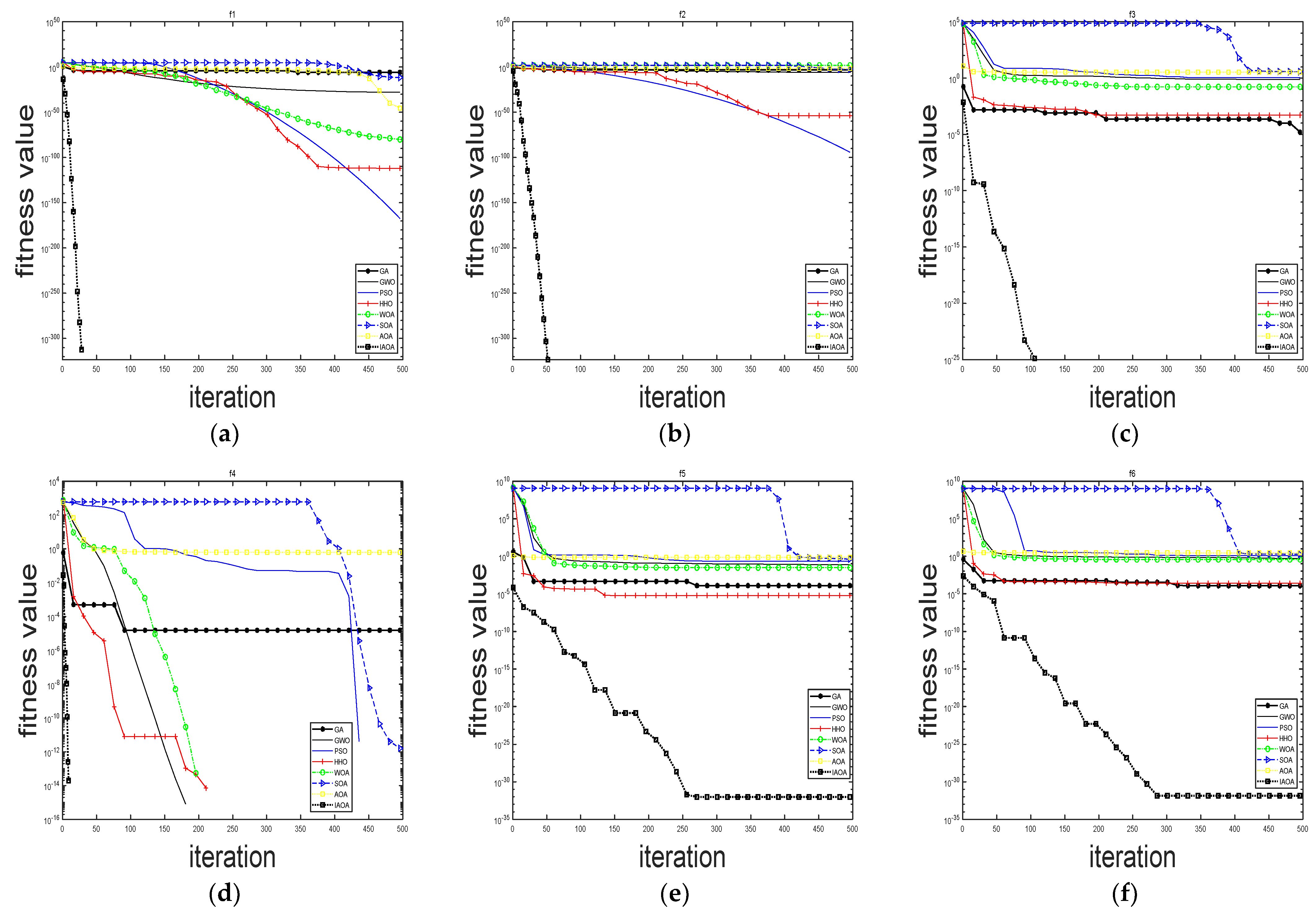
In addition, to evaluate the convergence performance of the proposed algorithms, Figure 2 shows the convergence plots of all algorithms for the six benchmark test functions (Dim = 30). From these convergence plots, it can be seen that IAOA converges to the global optimum faster than the other compared algorithms, which indicates that IAOA has a more powerful global search capability and has a faster convergence rate.

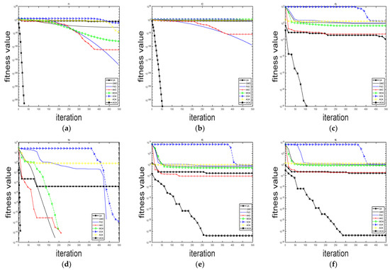
Figure 2. Function convergence curve: (a) f₁; (b) f₂; (c) f₃; (d) f₄; (e) f₅; (f) f₆.

5. Support Vector Machine (SVM) Parameter Optimization

The choice of parameters within the SVM is sensitive, and these parameters include penalty factors and kernel function parameters. Therefore, finding the optimal parameters is the key to improving the generalization ability of the SVM model. The traditional approach is to use a simple grid search, but this method is very slow and does not provide satisfactory results due to the large number of parameter combinations [60]. Another approach is the optimization of the parameters inside the SVM by metaheuristic algorithms. For example, Samadzadegan et al. [61] used a genetic algorithm to optimize the support vector machine and used it for a multi-classification problem; Bao et al. [62] used an improved Particle Swarm Algorithm to optimize the parameters of the support vector machine and achieved better classification results than grid search; Eswaramoorthy et al. [63] used the Gray Wolf Optimization algorithm to optimize the internal parameters of the support vector machine and achieved better classification accuracy. Although several metaheuristics have been applied to experiments on support vector machine parameter optimization, according to the “no free lunch” [64] theorem, there is no one optimization algorithm that can solve all optimization problems. Different datasets also affect the accuracy of SVM classification, and different metaheuristic algorithms for internal parameter search of SVMs for different datasets often lead to more satisfactory results, so the algorithm proposed in this paper is meaningful for support vector machine parameter optimization.

5.1. SVM Model and Classification Experimental Procedure

SVM is a typical machine learning algorithm for classification models. SVM achieves data classification by mapping low-dimensional vectors into a high-dimensional space and establishing optimal hyperplanes. By choosing a suitable kernel function, the linearly indistinguishable problem is transformed into a linearly divisible problem in the high-dimensional space. The SVM maps the input samples into the high-dimensional feature space by mapping functions α(x), kernel functions k(x_i, x_j) = α(x_i)·α(x_j), and according to the Lagrangian duality, the nonlinear support vector machine is transformed into solving the following convex quadratic programming problem:

$$\begin{array}{l}\underset{\alpha }{\min }\frac{1}{2}{\displaystyle \sum _{i=1}^M{\displaystyle \sum _{j=1}^M{\alpha }_i{\alpha }_j{y}_i{y}_{j}k(x_i,x_j)-{\displaystyle \sum _{i=1}^M{\alpha }_i}}}\\ s.t.\hspace{1em}{\displaystyle \sum _{i=1}^M{\alpha }_i{y}_j=0}\\ 0\le {\alpha }_{\mathrm{i}}\le C,i=1,2,\dots ,M\end{array}$$

(11)

where α_i is the Lagrangian multiplier. Using the quadratic programming method and the KKT condition, the special solution of the Lagrange multiplier is obtained, and the classification decision function is shown below:

$$f(x)=sign({\displaystyle \sum _{i=1}^M{\alpha }_i^{*}{y}_{i}k(x,x_i)+b^{*}})$$

(12)

The kernel function is usually chosen as the radial basis function (RBF), and its expression is shown below:

$$K(x,x_i)=\exp (-||x-x_i|{|}^2/2g^2)$$

(13)

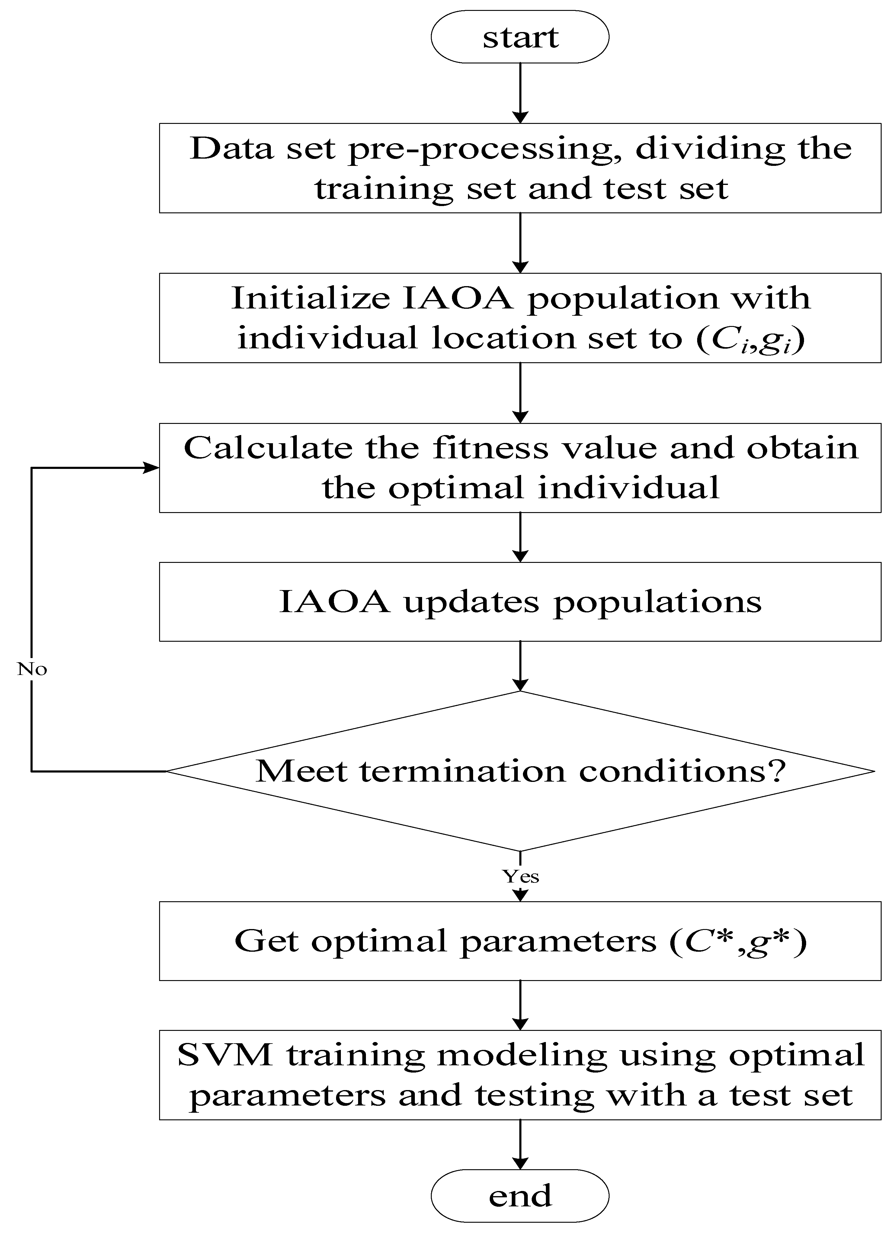
Obviously, in SVM parameter optimization, the penalty factor C and the kernel function parameter g have a great influence on the optimal model building of SVM. In this paper, IAOA is used to optimize the SVM parameters, and the penalty factor C and the kernel function parameter g are combined in an optimization search, and the classification accuracy of the training set is selected as the fitness function to evaluate the optimal (C, g) combination. The IAOA-SVM classification model is constructed, and its flowchart is shown in Figure 3.

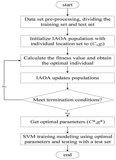
Figure 3. IAOA-SVM flow chart.

5.2. SVM Classification Test

To prevent the classification model from having too low generalization ability, we use 10-fold cross-validation, dividing the dataset into 10 parts, selecting one part in turn as the test set and the remaining nine parts as the training set to train the model and derive the accuracy of classification in the validation set. This process is performed for a total of 10 tests, and the average of the classification accuracy is finally obtained. In this experimental test, 18 datasets from the UCI Machine Learning Repository [65] were selected for classification testing. Specific information on the number of instances, features, and classes of these datasets is shown in Table 5. The IAOA method optimized SVM parameters were experimentally compared with the methods GA [2], GWO [10], PSO [11], HHO [13], WOA [14], SOA [16], and AOA [34] optimized SVM parameters using the 18 datasets, and for each dataset, the mean and standard deviation of 10 test validations were recorded for each method, thus verifying the different optimization performance of the different optimization methods. The search range of each optimization method was set to [10⁻⁶, 100] and the number of populations was set to 20. The parameters of each algorithm were set in accordance with Table 2.

Table 5. UCI dataset.

Dataset	Features	Instances	Classes
Balance	4	625	3
Breast cancer	9	277	2
DNA	180	2000	3
German	24	1000	2
glass	9	214	6
Heart	13	303	2
Ionosphere	34	351	2
Iris	4	150	3
zoo	16	101	7
Letter	16	5000	26
Liver	6	345	2
Vote	16	435	2
Waveform	21	5000	2
Pima	8	768	3
Segment	18	2310	7
Sonar	60	208	2
Wine	13	178	3
Vehicle	18	846	4

Classification accuracy (Number of correct classification results in the test sample/Number of test set samples) is the main metric to evaluate the performance of SVM parameter optimization, and Table 6 gives the accuracy, standard deviation, and accuracy ranking of the classification results for all algorithms for each dataset. Boxplot charts of the classification accuracy for all datasets are given in Figure 4 to evaluate the overall performance of all methods in a more visual way.

Table 6. Classification results.

Algorithm	GA		GWO		PSO		HHO
Dataset	Avg ± std	Rank	Avg ± std	Rank	Avg ± std	Rank	Avg ± std	Rank
Balance	97.10 ± 2.72	4	96.77 ± 3.72	8	97.10 ± 3.38	5	96.94 ± 4.06	7
Breast cancer	75.93 ± 7.86	7	78.52 ± 9.37	5	74.81 ± 9.85	8	78.52 ± 8.15	4
DNA	75.15 ± 19.58	7	93.94 ± 2.86	1	55.76 ± 4.56	8	91.21 ± 11.56	4
German	75.70 ± 5.50	7	78.60 + 3.60	1	74.60 ± 3.44	8	78.30 ± 4.14	5
glass	77.62 ± 8.11	4	77.14 ± 10.72	6	77.14 ± 7.71	7	77.62 ± 7.46	3
Heart	88.33 ± 7.24	1	85.33 ± 3.58	6	84.33 ± 4.73	8	87.67 ± 4.46	2
Ionosphere	93.71 ± 8.06	8	97.71 ± 2.25	2	94.57 ± 4.56	7	97.43 ± 2.5	3
Iris	97.33 ± 4.66	5	97.33 ± 3.44	3	96.67 ± 4.71	7	98.00 ± 3.22	2
zoo	93.00 ± 10.59	6	97.00 ± 4.83	1	85.00 ± 15.09	8	94.00 ± 6.99	4
Letter	88.21 ± 2.90	4	88.07 ± 1.78	6	87.93 ± 2.27	7	88.21 ± 3.30	5
Liver	75.00 ± 6.08	8	76.76 ± 9.85	7	76.76 ± 5.96	6	77.06 ± 6.47	5
Vote	94.65 ± 6.21	8	96.51 ± 3.51	2	94.65 ± 4.39	7	96.74 ± 2.50	1
Waveform	86.97 ± 5.35	8	89.39 ± 3.98	2	87.88 ± 3.71	7	89.09 ± 2.12	3
Pima	78.42 ± 5.27	7	79.21 ± 3.44	5	77.76 ± 3.94	8	79.34 ± 3.40	4
Segment	97.73 ± 1.92	5	97.27 ± 1.39	8	97.58 ± 2.49	6	97.73 ± 1.29	3
Sonar	90.53 ± 7.77	4	92.63 ± 5.66	2	87.37 ± 13.63	8	93.16 ± 7.04	1
Wine	98.82 ± 2.48	6	98.82 ± 2.48	7	98.24 ± 3.97	8	100.00 ± 0.00	1
Vehicle	84.09 ± 7.73	4	83.86 ± 5.91	5	83.41 ± 4.42	7	85.23 ± 5.59	2
Algorithm	WOA		SOA		AOA		IAOA
Dataset	Avg ± std	Rank	Avg ± std	Rank	Avg ± std	Rank	Avg ± std	Rank
Balance	97.26 ± 2.85	3	97.42 ± 1.56	2	96.94 ± 3.60	6	97.58 ± 2.97	1
Breast cancer	79.26 ± 8.04	3	79.26 ± 5.00	2	77.41 ± 6.40	6	79.63 ± 6.11	1
DNA	90.30 ± 13.54	6	92.27 ± 4.82	2	90.91 ± 6.06	5	91.52 ± 6.71	3
German	78.50 ± 3.10	2	78.30 ± 3.27	4	77.70 ± 3.59	6	78.40 ± 2.41	3
glass	76.67 ± 8.23	8	77.62 ± 5.52	2	77.62 ± 12.10	5	78.10 ± 5.59	1
Heart	87.33 ± 4.39	3	86.33 ± 4.57	4	85.33 ± 6.70	7	86.00 ± 6.05	5
Ionosphere	96.57 ± 2.95	5	97.14 ± 3.56	4	96.57 ± 3.76	6	98.00 ± 2.71	1
Iris	96.67 ± 3.51	8	97.33 ± 4.66	6	97.33 ± 3.44	4	98.67 ± 4.22	1
zoo	94.00 ± 8.43	5	96.00 ± 5.16	2	95.00 ± 5.27	3	93.00 ± 6.75	7
Letter	87.71 ± 1.50	8	88.57 ± 2.69	2	88.57 ± 3.55	3	88.79 ± 2.23	1
Liver	78.24 ± 4.64	2	79.41 ± 7.07	1	78.24 ± 6.82	3	77.94 ± 6.39	4
Vote	95.12 ± 7.31	5	96.05 ± 2.91	4	94.88 ± 4.63	6	96.28 ± 1.63	3
Waveform	88.48 ± 4.30	5	88.79 ± 4.69	4	88.03 ± 4.19	6	89.55 ± 2.62	1
Pima	79.87 ± 3.10	2	79.47 ± 4.69	3	79.08 ± 4.74	6	80.13 ± 4.45	1
Segment	97.73 ± 1.64	4	98.03 ± 1.61	1	97.88 ± 2.39	2	97.42 ± 1.76	7
Sonar	90.00 ± 9.75	5	92.11 ± 10.89	3	88.42 ± 8.15	7	88.95 ± 5.79	6
Wine	99.41 ± 1.86	2	99.41 ± 1.86	3	99.41 ± 1.86	4	99.41 ± 1.86	5
Vehicle	83.64 ± 4.77	6	84.77 ± 4.55	3	83.41 ± 6.25	8	86.36 ± 4.15	1

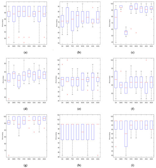
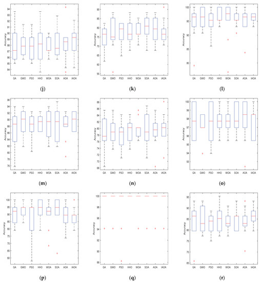
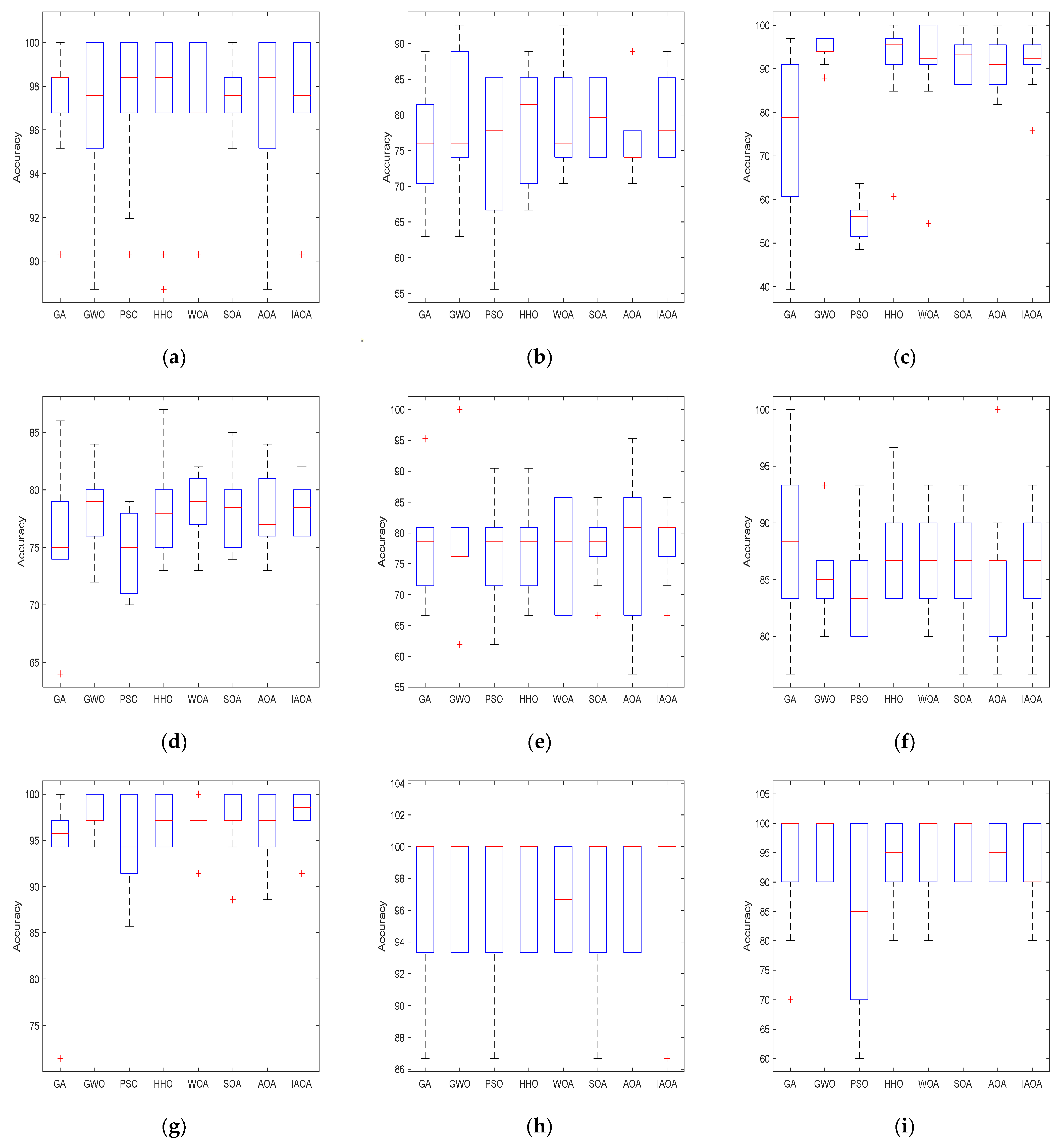
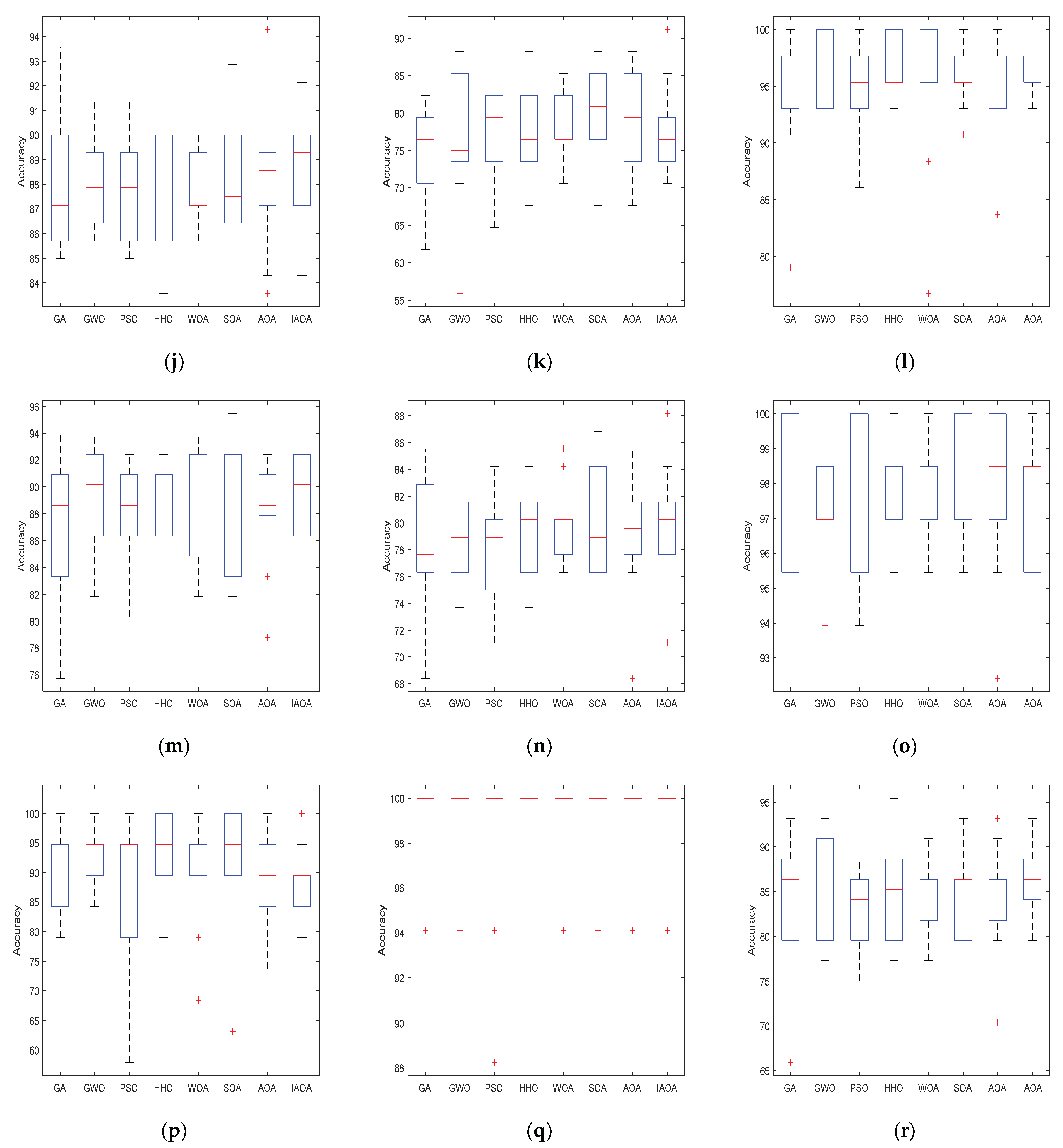
Figure 4. Boxplot charts for all comparison algorithms on 18 datasets: (a) Balance; (b) Breast Cancer; (c) DNA; (d) German; (e) glass; (f) Heart; (g) Ionosphere; (h) Iris; (i) zoo; (j) Letter; (k) Liver; (l) Vote; (m) Waveform; (n) Pima; (o) Segment; (p) Sonar; (q) Wine; (r) Vehicle.

According to the results in Table 6, it can be seen that the accuracy of IAOA’s classification results on all 18 datasets is ranked first on nine of them, which has obvious advantages in classification accuracy, and the accuracy of IAOA is equally competitive on the remaining nine datasets. For example, on the datasets DNA, German, and vote, IAOA’s accuracy is ranked in the top position. In addition, IAOA has a small standard deviation on all datasets, which shows the stability of the algorithm. In summary, IAOA has excellent classification accuracy and high stability; therefore, IAOA has strong practical performance. A line in the middle of the box plot indicates the median of the data, which reflects the average level of the data. The upper and lower lines of the box indicate the upper and lower quartiles of the data, which means that the box contains 50% of the data. Therefore, the width of the box reflects the fluctuation level of the data. There is a line above and below the box, sometimes representing the maximum and minimum values. The red “+” indicates outliers, which reflect abnormal data. It can be observed from Figure 4 that IAOA has good classification accuracy, as well as less fluctuation and fewer outliers, such as Figure 4d,e,g,h,j,l–n,r. Therefore, IAOA has a strong competitive edge in the experiments of support vector machine parameter optimization.

5.3. Handwritten Number Recognition Based on SVM Parameter Optimization

Recognition of handwritten numbers [66] has a wide range of applications in our social life. For example, banking, postal service, e-commerce, etc. However, unlike print, the recognition of handwriting is much higher than that of print because handwriting varies from person to person and its arbitrariness is greater. For this reason, this paper applies the proposed algorithm to support vector machine parameter optimization so that it can be applied to handwritten number recognition.

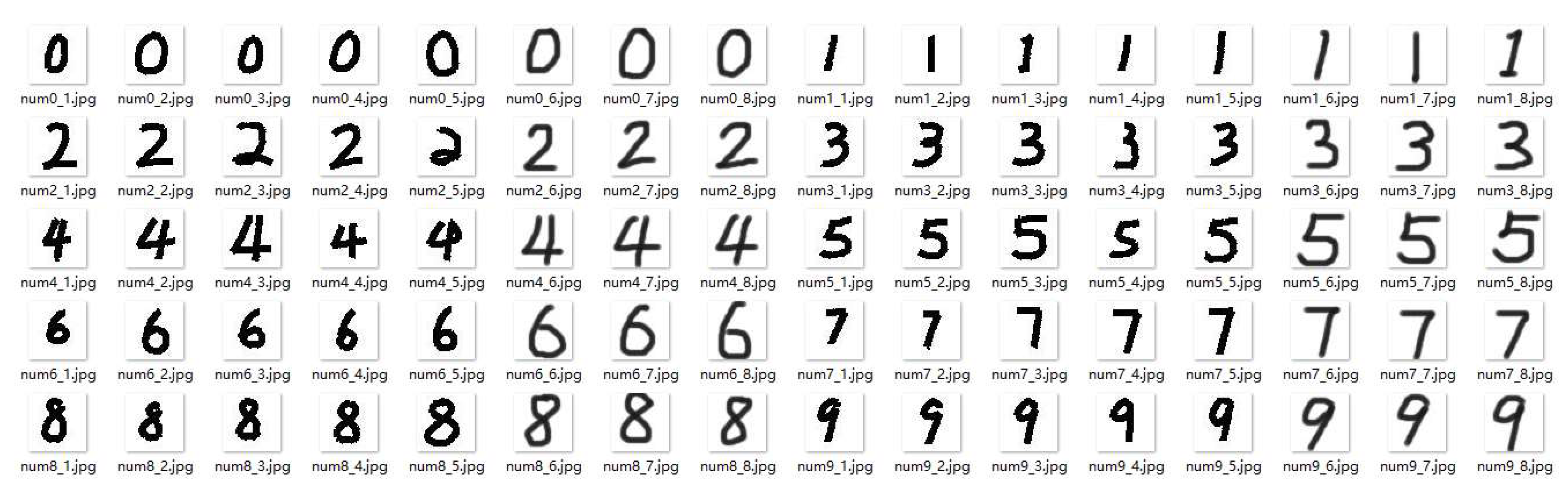
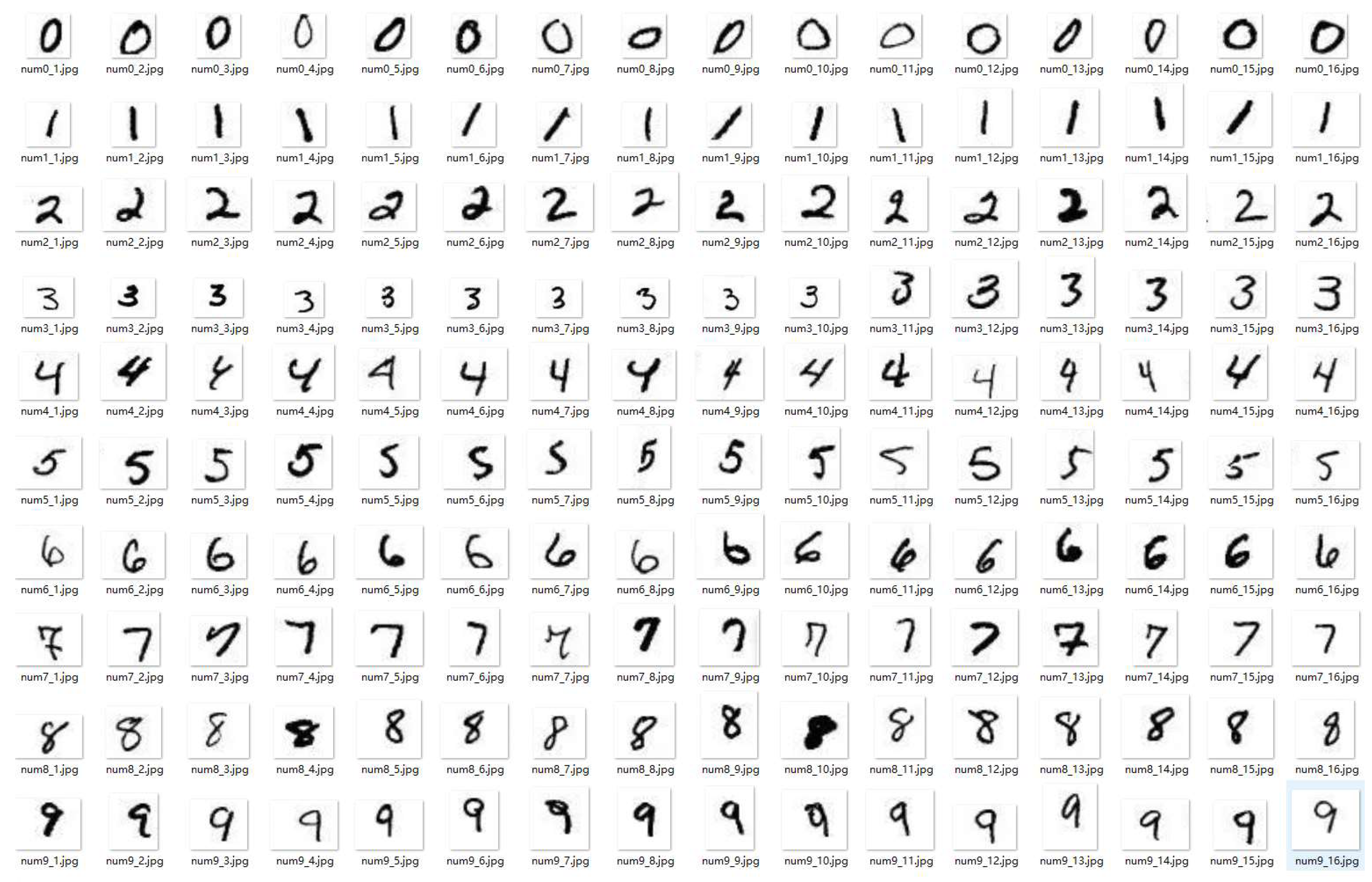
Eighty handwritten number images are selected as the training set, and each number has eight images. One of the training set sample images is shown as in Figure 5. A total of 160 handwritten number images of various shapes were selected as the test set, with 16 images for each number. The test set sample images are shown in Figure 6.

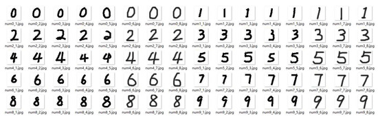
Figure 5. Sample images of the training set.

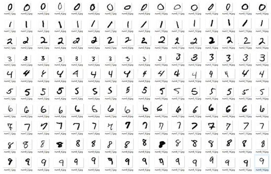
Figure 6. Sample images of the test set.

Handwriting Numeral Recognition Experiment

The handwritten number recognition experiment is mainly divided into the following steps: First, the training set images and the test set images are preprocessed in a standardized way: each image is inverse-colored and converted into a binary image; then, the largest region containing digits in the binary image is intercepted, and the intercepted region is converted into a standard 16×16 pixel image. Next, IAOA-SVM is constructed, RBF is selected as the kernel function, and the best combination of penalty factor and kernel function parameters (C, g) is found by using IAOA for SVM parameter search with the input training set images. Finally, the best training model is constructed using the best (C, g) combination, the input test set images, and the test set images are tested for classification. The algorithm IAOA proposed in this paper is compared with other methods (GA [2], GWO [10], PSO [11], HHO [13], WOA [14], SOA [16], AOA [34]) in numerical experiments to verify the practical performance of the algorithm proposed in this paper by comparing the accuracy rate in handwritten number recognition. Other test conditions are consistent with Section 5.3. Among them, Table 7 records the accuracy of handwritten number recognition for all algorithms after optimizing the SVM parameters and the best combination of penalty factor and kernel function parameters (C, g).

Table 7. Accuracy rate of handwritten digit recognition.

Parameters/Algorithms	GA	GWO	PSO	HHO	WOA	SOA	AOA	IAOA
C	1.0054	4.7506	98.2224	1.5743	11.0905	1.00 × 10−6	36.1315	53.5288
g	0.0100	0.0001	7.7435	0.0052	3.92 × 10−4	1.00 × 10−6	1.81 × 10−4	0.0109
Accuracy	98.375	96.875	100	99.375	96.875	88.75	98.75	100

The data in Table 7 show that the accuracy of IAOA and PSO is the highest in handwritten number recognition, which has obvious advantages compared with other algorithms, and the accuracy of IAOA has obvious improvement compared with AOA. Therefore, the algorithm proposed in this paper is more competitive in support vector machine parameter optimization and more applicable to handwritten number recognition, and the improvement of the AOA algorithm in this paper is meaningful and more practical ability.

6. Conclusions

To address the shortcomings of the basic AOA, an improved arithmetic optimization algorithm is proposed in this paper. Through the comparison of six benchmark functions, the proposed algorithm has a significant improvement in convergence speed, convergence accuracy, and the ability to jump out of the local optimum compared with AOA, and in the later experiments of support vector machine parameter optimization, the algorithm has excellent classification accuracy and has stronger practical ability. In the subsequent research, the algorithm is considered to be applied to more practical fields, such as feature selection, wireless sensor network node localization, and image segmentation.

References

- Hussain, K.; Mohd Salleh, M.N.; Cheng, S.; Shi, Y. Metaheuristic Research: A Comprehensive Survey—Artificial Intelligence Review. Artif. Intell. Rev. 2019, 52, 2191–2233. [Google Scholar] [CrossRef]
- Holland, J.H. Genetic algorithms. Sci. Am. 1992, 267, 66–73. [Google Scholar] [CrossRef]
- Storn, R.; Price, K. Differential evolution–a simple and efficient heuristic for global optimization over continuous spaces. J. Glob. Optim. 1997, 11, 341–359. [Google Scholar] [CrossRef]
- Hauschild, M.; Pelikan, M. An introduction and survey of estimation of distribution algorithms. Swarm Evol. Comput. 2011, 1, 111–128. [Google Scholar] [CrossRef]
- Adleman, L.M. Molecular computation of solutions to combinatorial problems. Science 1994, 266, 1021–1024. [Google Scholar] [CrossRef] [PubMed]
- Ferreira, C. Gene expression programming: A new adaptive algorithm for solving problems. Complex Syst. 2001, 13, 87–129. [Google Scholar]
- Neri, F.; Cotta, C. Memetic algorithms and memetic computing optimization: A literature review. Swarm Evol. Comput. 2012, 2, 1–14. [Google Scholar] [CrossRef]
- Reynolds, R.G.; Peng, B. Cultural algorithms: Computational modeling of how cultures learn to solve problems: An engineering example. Cybern. Syst. Int. J. 2005, 36, 753–771. [Google Scholar] [CrossRef]
- Karaboga, D.; Basturk, B. A powerful and efficient algorithm for numerical function optimization: Artificial bee colony (ABC) algorithm. J. Glob. Optim. 2007, 39, 459–471. [Google Scholar] [CrossRef]
- Mirjalili, S.; Mirjalili, S.M.; Lewis, A. Grey wolf optimizer. Adv. Eng. Softw. 2014, 69, 46–61. [Google Scholar] [CrossRef]
- Kennedy, J.; Eberhart, R. Particle swarm optimization. In Proceedings of the International Conference on Neural Networks, Perth, Australia, 27 November–1 December 1995; pp. 1942–1948. [Google Scholar]
- Gandomi, A.H.; Yang, X.S.; Alavi, A.H. Cuckoo search algorithm: A metaheuristic approach to solve structural optimization problems. Eng. Comput. 2013, 29, 17–35. [Google Scholar] [CrossRef]
- Heidari, A.A.; Mirjalili, S.; Faris, H.; Aljarah, I.; Mafarja, M.; Chen, H. Harris hawks optimization: Algorithm and applications. Future Gener. Comput. Syst. 2019, 97, 849–872. [Google Scholar] [CrossRef]
- Mirjalili, S.; Lewis, A. The whale optimization algorithm. Adv. Eng. Softw. 2016, 95, 51–67. [Google Scholar] [CrossRef]
- Li, S.; Chen, H.; Wang, M.; Heidari, A.A.; Mirjalili, S. Slime mould algorithm: A new method for stochastic optimization. Future Gener. Comput. Syst. 2020, 111, 300–323. [Google Scholar] [CrossRef]
- Dhiman, G.; Kumar, V. Seagull optimization algorithm: Theory and its applications for large-scale industrial engineering problems. Knowl. Based Syst. 2019, 165, 169–196. [Google Scholar] [CrossRef]
- Hashim, F.A.; Houssein, E.H.; Mabrouk, M.S.; Al-Atabany, W.; Mirjalili, S. Henry gas solubility optimization: A novel physics-based algorithm. Future Gener. Comput. Syst. 2019, 101, 646–667. [Google Scholar] [CrossRef]
- Erol, O.K.; Eksin, I. A new optimization method: Big bang–big crunch. Adv. Eng. Softw. 2006, 37, 106–111. [Google Scholar] [CrossRef]
- Mirjalili, S.; Mirjalili, S.M.; Hatamlou, A. Multi-verse optimizer: A nature-inspired algorithm for global optimization. Neural Comput. Appl. 2016, 27, 495–513. [Google Scholar] [CrossRef]
- Abedinpourshotorban, H.; Shamsuddin, S.M.; Beheshti, Z.; Jawawi, D.N. Electromagnetic field optimization: A physics-inspired metaheuristic optimization algorithm. Swarm Evol. Comput. 2016, 26, 8–22. [Google Scholar] [CrossRef]
- Rashedi, E.; Nezamabadi-Pour, H.; Saryazdi, S. GSA: A gravitational search algorithm. Inf. Sci. 2009, 179, 2232–2248. [Google Scholar] [CrossRef]
- Rao, R.V.; Savsani, V.J.; Vakharia, D.P. Teaching–learning-based optimization: An optimization method for continuous non-linear large scale problems. Inf. Sci. 2012, 183, 1–15. [Google Scholar] [CrossRef]
- Geem, Z.W.; Kim, J.H.; Loganathan, G.V. A new heuristic optimization algorithm: Harmony search. Simulation 2001, 76, 60–68. [Google Scholar] [CrossRef]
- Talatahari, S.; Azar, B.F.; Sheikholeslami, R.; Gandomi, A. Imperialist competitive algorithm combined with chaos for global optimization. Commun. Nonlinear Sci. Numer. Simul. 2012, 17, 1312–1319. [Google Scholar] [CrossRef]
- Li, J.; Tan, Y. A comprehensive review of the fireworks algorithm. ACM Comput. Surv. CSUR 2019, 52, 1–28. [Google Scholar] [CrossRef]
- Zhang, Q.; Wang, R.; Yang, J.; Ding, K.; Li, Y.; Hu, J. Collective decision optimization algorithm: A new heuristic optimization method. Neurocomputing 2017, 221, 123–137. [Google Scholar] [CrossRef]
- Abualigah, L.; Diabat, A. A comprehensive survey of the Grasshopper optimization algorithm: Results, variants, and applications. Neural Comput. Appl. 2020, 32, 15533–15556. [Google Scholar] [CrossRef]
- Zhang, J.; Gong, D.; Zhang, Y. A niching PSO-based multi-robot cooperation method for localizing odor sources. Neurocomputing 2014, 123, 308–317. [Google Scholar] [CrossRef]
- Ma, D.; Ma, J.; Xu, P. An adaptive clustering protocol using niching particle swarm optimization for wireless sensor networks. Asian J. Control 2015, 17, 1435–1443. [Google Scholar] [CrossRef]
- Mehmood, S.; Cagnoni, S.; Mordonini, M.; Khan, S.A. An embedded architecture for real-time object detection in digital images based on niching particle swarm optimization. J. Real Time Image Process. 2015, 10, 75–89. [Google Scholar] [CrossRef]
- Gholami, M.; Alashti, R.A.; Fathi, A. Optimal design of a honeycomb core composite sandwich panel using evolutionary optimization algorithms. Compos. Struct. 2016, 139, 254–262. [Google Scholar] [CrossRef]
- Mafarja, M.; Aljarah, I.; Heidari, A.A.; Hammouri, A.I.; Faris, H.; Al-Zoubi, A.M.; Mirjalili, S. Evolutionary population dynamics and grasshopper optimization approaches for feature selection problems. Knowl. Based Syst. 2018, 145, 25–45. [Google Scholar] [CrossRef]
- Tharwat, A.; Houssein, E.H.; Ahmed, M.M.; Hassanien, A.E.; Gabel, T. MOGOA algorithm for constrained and unconstrained multi-objective optimization problems. Appl. Intell. 2018, 48, 2268–2283. [Google Scholar] [CrossRef]
- Abualigah, L.; Diabat, A.; Mirjalili, S.; Abd Elaziz, M.; Gandomi, A.H. The arithmetic optimization algorithm. Comput. Methods Appl. Mech. Eng. 2021, 376, 113609. [Google Scholar] [CrossRef]
- Khatir, S.; Tiachacht, S.; Le Thanh, C.; Ghandourah, E.; Mirjalili, S.; Wahab, M.A. An improved Artificial Neural Network using Arithmetic Optimization Algorithm for damage assessment in FGM composite plates. Compos. Struct. 2021, 273, 114287. [Google Scholar] [CrossRef]
- Deepa, N.; Chokkalingam, S.P. Optimization of VGG16 utilizing the Arithmetic Optimization Algorithm for early detection of Alzheimer’s disease. Biomed. Signal Process. Control 2022, 74, 103455. [Google Scholar] [CrossRef]
- Almalawi, A.; Khan, A.I.; Alsolami, F.; Alkhathlan, A.; Fahad, A.; Irshad, K.; Alfakeeh, A.S.; Qaiyum, S. Arithmetic optimization algorithm with deep learning enabled airborne particle-bound metals size prediction model. Chemosphere 2022, 303, 134960. [Google Scholar] [CrossRef]
- Ahmadi, B.; Younesi, S.; Ceylan, O.; Ozdemir, A. The Arithmetic Optimization Algorithm for Optimal Energy Resource Planning. In Proceedings of the 2021 56th International Universities Power Engineering Conference (UPEC), Middlesbrough, UK, 31 August 2021–3 September 2021; pp. 1–6. [Google Scholar]
- Bhat, S.J.; Santhosh, K.V. A localization and deployment model for wireless sensor networks using arithmetic optimization algorithm. Peer Peer Netw. Appl. 2022, 15, 1473–1485. [Google Scholar] [CrossRef]
- Kaveh, A.; Hamedani, K.B. Improved arithmetic optimization algorithm and its application to discrete structural optimization. Structures 2022, 35, 748–764. [Google Scholar] [CrossRef]
- Agushaka, J.O.; Ezugwu, A.E. Advanced arithmetic optimization algorithm for solving mechanical engineering design problems. PLoS ONE 2021, 16, e0255703. [Google Scholar] [CrossRef]
- Premkumar, M.; Jangir, P.; Kumar, B.S.; Sowmya, R.; Alhelou, H.H.; Abualigah, L.; Yildiz, A.R.; Mirjalili, S. A new arithmetic optimization algorithm for solving real-world multiobjective CEC-2021 constrained optimization problems: Diversity analysis and validations. IEEE Access 2021, 9, 84263–84295. [Google Scholar] [CrossRef]
- Zheng, R.; Jia, H.; Abualigah, L.; Liu, Q.; Wang, S. Deep ensemble of slime mold algorithm and arithmetic optimization algorithm for global optimization. Processes 2021, 9, 1774. [Google Scholar] [CrossRef]
- Abualigah, L.; Diabat, A.; Sumari, P.; Gandomi, A. A novel evolutionary arithmetic optimization algorithm for multilevel thresholding segmentation of COVID-19 ct images. Processes 2021, 9, 1155. [Google Scholar] [CrossRef]
- Ibrahim, R.A.; Abualigah, L.; Ewees, A.A.; Al-Qaness, M.A.A.; Yousri, D.; Alshathri, S.; Elaziz, M.A. An electric fish-based arithmetic optimization algorithm for feature selection. Entropy 2021, 23, 1189. [Google Scholar] [CrossRef] [PubMed]
- Wang, R.B.; Wang, W.F.; Xu, L.; Pan, J.S.; Chu, S.C. An Adaptive Parallel Arithmetic Optimization Algorithm for Robot Path Planning. Available online: https://www.hindawi.com/journals/jat/2021/3606895/ (accessed on 6 July 2022).
- Ewees, A.A.; Al-qaness, M.A.; Abualigah, L.; Oliva, D.; Algamal, Z.Y.; Anter, A.M.; Ibrahim, R.A.; Ghoniem, R.M.; Elaziz, M.A. Boosting arithmetic optimization algorithm with genetic algorithm operators for feature selection: Case study on cox proportional hazards model. Mathematics 2021, 9, 2321. [Google Scholar] [CrossRef]
- Abualigah, L.; Diabat, A. Improved multi-core arithmetic optimization algorithm-based ensemble mutation formultidisciplinary applications. J. Intell. Manuf. 2022, 1–42. [Google Scholar] [CrossRef]
- Khodadadi, N.; Snasel, V.; Mirjalili, S. Dynamic arithmetic optimization algorithm for truss optimization under natural frequency constraints. IEEE Access 2022, 10, 16188–16208. [Google Scholar] [CrossRef]
- Mahajan, S.; Abualigah, L.; Pandit, A.K.; Altalhi, M. Hybrid Aquila optimizer with arithmetic optimization algorithm for global optimization tasks. Soft Comput. 2022, 26, 4863–4881. [Google Scholar] [CrossRef]
- Li, X.-D.; Wang, J.-S.; Hao, W.-K.; Zhang, M.; Wang, M. Chaotic arithmetic optimization algorithm. Appl. Intell. 2022, 1–40. [Google Scholar] [CrossRef]
- Elaziz, M.A.; Abualigah, L.; Ibrahim, R.A.; Attiya, I. IoT Workflow Scheduling Using Intelligent Arithmetic Optimization Algorithm in Fog Computing. Comput. Intell. Neurosci. 2022, 2021, 9114113. Available online: https://www.hindawi.com/journals/cin/2021/9114113/ (accessed on 15 July 2022). [CrossRef]
- Cortes, C.; Vapnik, V. Support-vector networks. Mach. Learn. 1995, 20, 273–297. [Google Scholar] [CrossRef]
- Zhang, H.; Berg, A.C.; Maire, M.; Malik, J. SVM-KNN: Discriminative nearest neighbor classification for visual category recognition. In Proceedings of the 2006 IEEE Computer Society Conference on Computer Vision and Pattern Recognition (CVPR’06), New York, NY, USA, 17–22 June 2006; pp. 2126–2136. [Google Scholar]
- Jerlin Rubini, L.; Perumal, E. Efficient classification of chronic kidney disease by using multi-kernel support vector machine and fruit fly optimization algorithm. Int. J. Imaging Syst. Technol. 2020, 30, 660–673. [Google Scholar] [CrossRef]
- Lin, G.Q.; Li, L.L.; Tseng, M.; Liu, H.-M.; Yuan, D.-D.; Tan, R.R. An improved moth-flame optimization algorithm for support vector machine prediction of photovoltaic power generation. J. Clean. Prod. 2020, 253, 119966. [Google Scholar] [CrossRef]
- Momin, J.; Xin-She, Y. A literature survey of benchmark functions for global optimization problems. J. Math. Model. Numer. Optim. 2013, 4, 150–194. [Google Scholar]
- Shi, Y.; Eberhart, R. A modified particle swarm optimizer. In Proceedings of the 1998 IEEE International Conference on Evolutionary Computation Proceedings, Anchorage, AK, USA, 4–9 May 1998; pp. 69–73. [Google Scholar]
- Fan, H.Y.; Lampinen, J. A trigonometric mutation operation to differential evolution. J. Glob. Optim. 2003, 27, 105–129. [Google Scholar] [CrossRef]
- Güraksın, G.E.; Haklı, H.; Uğuz, H. Support vector machines classification based on particle swarm optimization for bone age determination. Appl. Soft Comput. 2014, 24, 597–602. [Google Scholar] [CrossRef]
- Samadzadegan, F.; Soleymani, A.; Abbaspour, R.A. Evaluation of genetic algorithms for tuning SVM parameters in multi-class problems. In Proceedings of the 2010 11th International Symposium on Computational Intelligence and Informatics (CINTI), Budapest, Hungary, 18–20 November 2010; pp. 323–328. [Google Scholar]
- Bao, Y.; Hu, Z.; Xiong, T. A PSO and pattern search based memetic algorithm for SVMs parameters optimization. Neurocomputing 2013, 117, 98–106. [Google Scholar] [CrossRef]
- Eswaramoorthy, S.; Sivakumaran, N.; Sekaran, S. Grey Wolf Optimization Based Parameter Selection for Support Vector Machines. COMPEL Int. J. Comput. Math. Electr. Electron. Eng. 2016, 35, 1513–1523. [Google Scholar] [CrossRef]
- Wolpert, D.H.; Macready, W.G. No free lunch theorems for optimization. IEEE Trans. Evol. Comput. 1997, 1, 67–82. [Google Scholar] [CrossRef]
- Frank, A.; Asuncion, A. UCI Machine Learning Repository. 2010. Available online: http://archive.ics.uci.edu/ml (accessed on 15 July 2022).
- Bin, Z.; Yong, L.; Shao-Wei, X. Support vector machine and its application in handwritten numeral recognition. In Proceedings of the 15th International Conference on Pattern Recognition, Barcelona, Spain, 3–7 September 2000; pp. 720–723. [Google Scholar]
Publisher’s Note: MDPI stays neutral with regard to jurisdictional claims in published maps and institutional affiliations. |
© 2022 by the authors. Licensee MDPI, Basel, Switzerland. This article is an open access article distributed under the terms and conditions of the Creative Commons Attribution (CC BY) license (https://creativecommons.org/licenses/by/4.0/).