Mixed Convection Flow of Water Conveying Graphene Oxide Nanoparticles over a Vertical Plate Experiencing the Impacts of Thermal Radiation

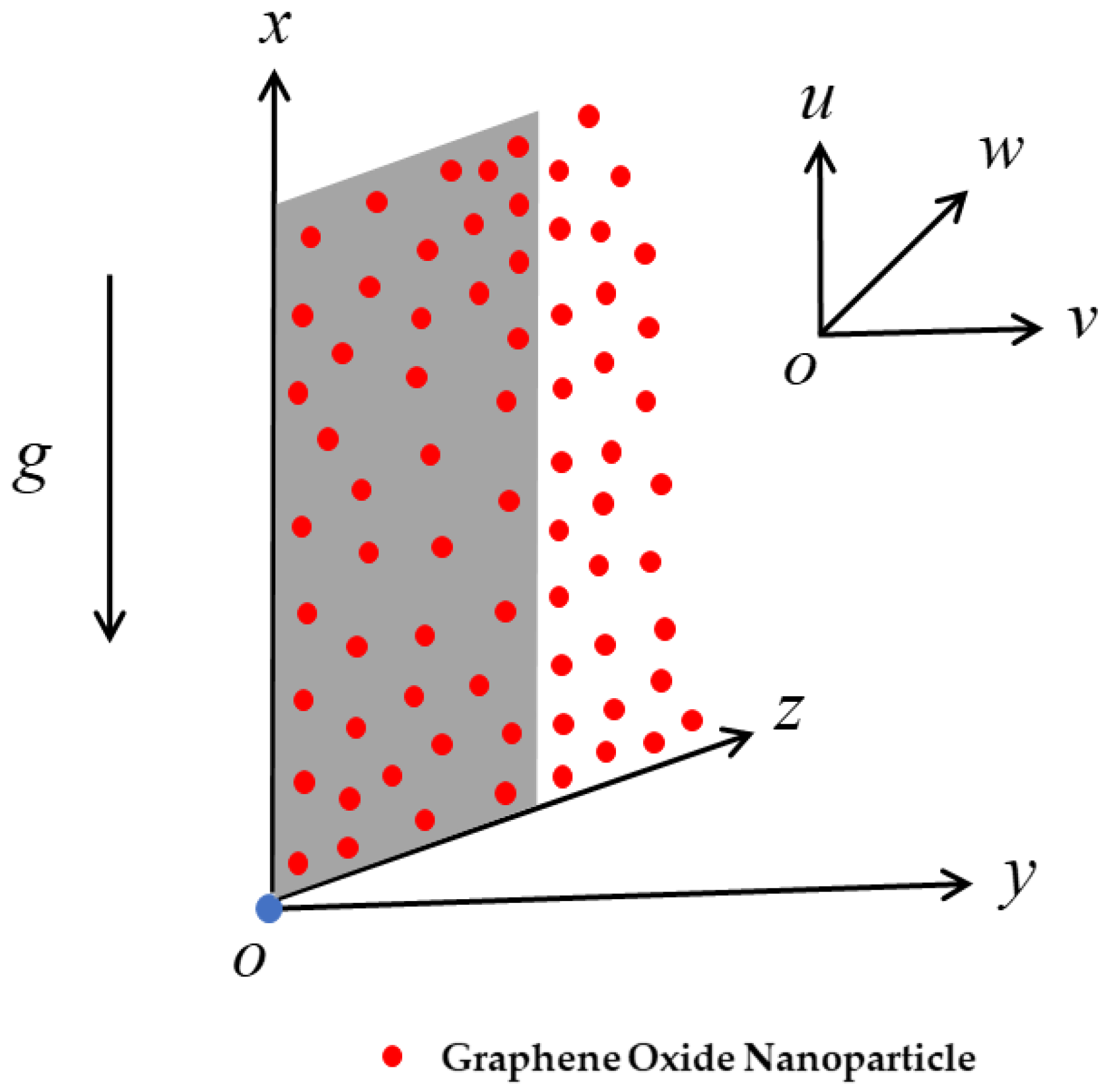
Abstract

Water has drawn a lot of interest as a manufacturing lubricant since it is affordable, eco-friendly, and effective. Due to their exceptional mechanical qualities, water solubility, and variety of application scenarios, graphene oxide (GO)-based materials have the potential to increase the lubricant performance of water. The idea of this research was to quantify the linear 3D radiative stagnation-point flow induced by nanofluid through a vertical plate with a buoyancy or a mixed convection effect. The opposing, as well as the assisting, flows were considered in the model. The leading partial differential equations (PDEs) were transformed into dimensionless similarity equations, which were then solved numerically via a bvp4c solver. The influences of various physical constraints on the fluid flow and thermal properties of the nanofluid were investigated and are discussed. Water-based graphene oxide nanoparticles were considered in this study. The numerical outcomes indicated that multiple solutions were obtained in the case of the opposing flow (λ < 0). The critical values increased as the nanoparticle volume fraction became stronger. Furthermore, as the nanoparticles increased in strength, the friction factor increased and the heat transfer quickened. The radiation factor escalated the heat transfer in both solutions. In addition, a temporal stability analysis was also undertaken to verify the results, and it was observed that the branch of the first outcome became physically reliable (stable) whilst the branch of the second outcome became unstable, as time passed.

1. Introduction

The thermal properties of convectional heat transfers are critical in industrial and engineering applications. Due to their low thermal conductivity, various traditional fluids, such as oil, water, and kerosene, do not deliver heat effectively. Various forms of nanoparticles can be embedded into traditional fluids to improve heat transport. The resulting solution is known as nanofluid, and the presence of nanoparticles in the fluid improves the thermal conductivity, as well as the heat transfer rate. Choi [1] introduced the word “nanofluid” for the first time in 1995. Nanofluids are mixtures of liquid comprised of tiny sized particles that are utilized for the enhancement of thermal conductivity. Ellahi et al. [2] explored the role of magnetic and slip effects on non-Newtonian nanofluid flow across a porous coaxial cylinder. The influence of a magnetic field on the free convective flow of a nanoparticle over a stretching porous sheet was inspected by Rosmila et al. [3]. They discovered that the volume fraction of the nanoparticles and the thermal stratification effects increased the regular heat transport. Sheikholeslami et al. [4] used Galerkin and least-squares methods to investigate the magnetized flow via a semi-porous channel induced by nanofluid and obtained an analytic solution. They found that the influence of the magnetic constraint on the thickness of the velocity boundary layer was minimal. Javaherdeh and Ashorynejad [5] investigated the force-convection magnetized flow induced by nanofluid through a filled, partially porous channel and utilized the lattice Boltzmann method. They revealed that the average Nusselt number increases as a result of increasing the volume fraction, and there was also a slow enhancement due to magnetic influence. The influence of heat transfer on the coflowing fluid flow in a nanofluid across a porous moving surface was investigated by Noor et al. [6]. Wang and Su [7] conducted an experiment-type investigation on nanoliquid flow scorching-energy transfer through an orthogonal tube with modified pressure conditions. Sandeep and Malvandi [8] inspected the magnetic impact on the thin fluid flow of water-based graphene oxide nanoparticles induced by non-Newtonian fluid. The features of the heat transfer and fluid flow resulting from the use of water-based graphene oxide were examined by Zuhra et al. [9]. Ghosh and Mukhopadhyay [10] investigated the heat transfer characteristics for forced convective flow-expressing nanofluid on a moving plate utilizing a heat sink/source and porous medium. Xue et al. [11] investigated water-based graphene oxide material and presented the experimental results. Recently, Khan et al. [12] investigated the features of mixed convective magnetic flow and heat transport of a nanofluid passed through an irregular shrinking/stretching heated plate and provided double solutions.

Mixed convection flow is critical in several processes in engineering fields. The combination of free and forced convective flows is involved in many transport mechanisms, such as solar collectors, heat exchangers, electronics equipment, and nuclear reactors. Mixed convective flows are vital when the buoyancy force owing to the difference in temperature between the solid surface and the free stream becomes large, affecting the thermal fields and the flow significantly. Ramachandran et al. [13] studied the 2D flow near a stagnation point subject to mixed convection across a vertical surface, taking into account the variations in the arbitrary surface heat flux, as well as the arbitrary wall temperature. They indicated that a region of reverse flow formed in the region of opposing flow, and double solutions were discovered in that regime flow for a specific range of the mixed convection parameter. This work was extended by Devi et al. [14] to an example of unsteady flows, where the instabilities in the flow and temperature were exacerbated by the time-dependent velocity of the free stream. Bachok et al. [15] investigated the features of stagnation-point flow and heat transfer through a flat vertical plate, incorporating mixed convection and an anisotropic fluid immersed in porous media. They established that anisotropy had the effect of expanding the possible choices for the modified mixed convective parameters that could produce results. Bhattacharyya et al. [16] inspected the influence of slip on buoyancy flow through a vertical surface. They observed that the dimensionless temperature and velocity were overshot due to slip and the mixed convection parameters. The impact of the convective condition on mixed convective flow from a vertical cone saturated in a porous media was inspected by Rosali et al. [17]. They explored these two dissimilar branches’ outcomes in a situation of buoyancy-opposing flow. The effect of heat generation on the mixed convective flow of a non-Newtonian nanofluid through a circular heated cylinder was scrutinized by Mahat et al. [18]. Khan and Rasheed et al. [19] numerically inspected the impact of MHD on the mixed convective flow and heat transfer of a Maxwellian nanofluid through an aligned plate moving horizontally. Bouslimi et al. [20] inspected the magnetic flow induced by nanomaterials with mixed convection under an irregularly extending heated surface.

Following the literature review, we can assert that the problem considered here is how to augment heat transfer fluids using mixed-convection 3D flows induced by a nanofluid through a vertical plate, which is a problem that has been not discussed before. In addition, the influence of radiation and the stagnation-point flow is also discussed. The goal was to improve the quality of the thermal conductivity of regular fluid to achieve improved heat transfer with portable density for the heat exchangers used in modern thermal processes. Graphical results were obtained using numerical simulation undertaken by transforming PDEs into ODEs using appropriate transformations. A stability analysis was also undertaken to explore the stable solutions.

2. Mathematical Formulation

Consider a mixed convection boundary layer stagnation-point flow of a linear three-dimensional nanofluid induced by a vertical plate located along the $xy$-plane, as depicted in Figure 1. The background of the physical model can be bounded with the help of Cartesian coordinates $x$, $y$, and $z$, and the flow enactment occupies the domain $z\ge 0$. Additionally, in this flow model, we considered that the density varies linearly along with the temperature; hence, Rosseland’s linear thermal radiation $q_r$ was assimilated to analyze the heat transfer behavior. In this examination of the coordinate system, the velocity at the plate was assumed to be zero, while the velocity of the far field or free stream is signified by the components $u_e=ax$, $v_e=by$, and $w_e=-(a+b)z$, where $a$ and $b$ are arbitrary constants. Moreover, the nature of the stagnation point (SP) is determined by the signs and relative magnitudes of $a$ and $b$. If the normal component of the mainstream velocity is oriented toward the wall surface of the plate—that is, if $\left(a+b\right)>0$—we speak about a point of attachment in this study. A point of separation is used in the opposite situation. The stagnation point is called a nodal point if $a$ and $b$ have the same sign; otherwise, it is called a saddle point. Furthermore, the variable temperature at the plate and the far-field constant temperature are denoted $T_w\left(x\right)$ and $T_{\infty }$, respectively. For the heated plate (buoyancy-assisting flow), the temperature at the plate is greater than the requisite far-field temperature—i.e., $T_w\left(x\right)>T_{\infty }$—while the case in which $T_w\left(x\right)<T_{\infty }$ represents the cooling plate (buoyancy-opposing flow). For thermal enhancement, graphene oxide (GO) was incorporated into the base fluid (water) to form the posited nanofluid.

Figure 1. The configuration model for the nanofluid flow and embedded coordinate system.

Under these assumptions, the continuity, momentum, and energy equations of the nanofluid can be written as (Devi and Devi [21]):

$$\frac{\partial u}{\partial x}+\frac{\partial v}{\partial y}+\frac{\partial w}{\partial z}=0,$$

(1)

$$u\frac{\partial u}{\partial x}+v\frac{\partial u}{\partial y}+w\frac{\partial u}{\partial z}-a^{2}x=\frac{{\mu }_{nf}}{{\rho }_{nf}}\frac{{\partial }^{2}u}{\partial z^2}+\frac{g}{{\rho }_{nf}}{\left(\rho {\beta }_a\right)}_{nf}\left(T-T_{\infty }\right),$$

(2)

$$u\frac{\partial v}{\partial x}+v\frac{\partial v}{\partial y}+w\frac{\partial v}{\partial z}-b^{2}y=\frac{{\mu }_{nf}}{{\rho }_{nf}}\frac{{\partial }^{2}v}{\partial z^2}+\frac{g}{{\rho }_{nf}}{\left(\rho {\beta }_a\right)}_{nf}\left(T-T_{\infty }\right),$$

(3)

$$u\frac{\partial T}{\partial x}+v\frac{\partial T}{\partial y}+w\frac{\partial T}{\partial z}=\frac{k_{nf}}{{\left(\rho c_p\right)}_{nf}}\frac{{\partial }^{2}T}{\partial z^2}-\frac{1}{{\left(\rho c_p\right)}_{nf}}\frac{\partial q_r}{\partial z},$$

(4)

subject to the boundary conditions (BCs):

$$\left\{\begin{array}{l}u=0,v=0,w=0,T=T_w\left(x\right),atz=0\\ u\to u_e,v\to v_e,w\to w_e,T\to T_{\infty },asz\to \infty .\end{array}\right.$$

(5)

Here, $w$, $v$, and $u$ are the velocity components of the nanofluid along the relative $z$, $y$, and $x$ axes, $T$ is the temperature of the nanofluid, and $g$ is the acceleration due to gravity.

Additionally, the mathematical symbols used in the governing Equations (2)–(4) are the absolute viscosity ${\mu }_{nf}$, the thermal conductivity $k_{nf}$, the density ${\rho }_{nf}$, the thermal expansion coefficient ${\left(\rho {\beta }_a\right)}_{nf}$, and the specific heat capacitance ${\left(\rho c_p\right)}_{nf}$ of the nanofluid, which are given by:

$$\frac{{\mu }_{nf}}{{\mu }_f}=\frac{1}{{\left(1-{\phi }_{GO}\right)}^{2.5}},$$

(6)

$$\frac{k_{nf}}{k_f}=\frac{\left(k_{GO}+2k_f\right)-2{\phi }_{GO}\left(k_f-k_{GO}\right)}{\left(k_{GO}+2k_f\right)+{\phi }_{GO}\left(k_f-k_{GO}\right)},$$

(7)

$$\frac{{\rho }_{nf}}{{\rho }_f}={\phi }_{GO}\left(\frac{{\rho }_{GO}}{{\rho }_f}\right)+\left(1-{\phi }_{GO}\right),$$

(8)

$$\frac{{\left(\rho {\beta }_a\right)}_{nf}}{{\left(\rho {\beta }_a\right)}_f}={\phi }_{GO}\left(\frac{{\left(\rho {\beta }_a\right)}_{GO}}{{\left(\rho {\beta }_a\right)}_f}\right)+\left(1-{\phi }_{GO}\right),$$

(9)

$$\frac{{\left(\rho c_p\right)}_{nf}}{{\left(\rho c_p\right)}_f}={\phi }_{GO}\left(\frac{{\left(\rho c_p\right)}_{GO}}{{\left(\rho c_p\right)}_f}\right)+\left(1-{\phi }_{GO}\right).$$

(10)

In the above equations (Equations (6)–(10)), the notation ${\phi }_{GO}$ is called the solid volume fraction of the nanoparticles, whereas the particular value of ${\phi }_{GO}=0$ corresponds to the base fluid (water). In addition, the symbols $k_f$, $k_{GO}$, ${\mu }_f$, ${\mu }_{GO}$, ${\rho }_f$, ${\rho }_{GO}$, ${\beta }_{af}$, and ${\beta }_{aGO}$ signify the relative thermal conductivity, viscosity, density, and coefficient of the TE of the normal-based fluid and the solid volume fraction of the nanoparticles, respectively. Furthermore, ${\left(c_p\right)}_f$ and ${\left(c_p\right)}_{GO}$ are the heat capacity at the uniform or constant pressure of the pure fluid and the solid nanomaterial volume fraction, respectively. The thermo-physical experimental data of the normal-based fluid and the graphene oxide nanoparticles are given in Table 1.

Table 1. The thermo-physical properties of the water/GO nanofluid [22].

Properties	${\mathit{c}}_{\mathit{p}}\left(\mathbf{J}/\mathbf{kgK}\right)$	$\mathit{\rho }\left({\mathbf{kg}/\mathbf{m}}^3\right)$	${\mathit{\beta }}_{\mathit{a}}\times {10}^{-5}\left({\mathbf{K}}^{-1}\right)$	$\mathit{k} \left(\mathbf{W}/\mathbf{mk}\right)$	Pr
Water	4179	997.1	21	0.613	6.2
GO	717	1800	$2.8\times {10}^{-4}$	5000	-

By making use of Rosseland’s approximation, the expression for the radiative heat flux $q_r$ can be articulated in the following form [23,24,25]:

$$q_r=-\frac{4{\sigma }^{*}}{3k^{*}}\frac{\partial T^4}{\partial z},$$

(11)

where $T^4\approx T_{\infty }^4+4T_{\infty }^3\left(T-T_{\infty }\right)$.

Using Equation (11) for the last term of Equation (4), we get:

$$\frac{1}{{\left(\rho c_p\right)}_{nf}}\frac{\partial q_r}{\partial z}=\frac{-1}{{\left(\rho c_p\right)}_{nf}}\frac{16{\sigma }^{*}{T}_{\infty }^3}{3k^{*}}\frac{{\partial }^{2}T}{\partial z^2}.$$

(12)

Then, writing the energy equation in a more simplified, closed form than putting Equation (12) into Equation (4), we get:

$$u\frac{\partial T}{\partial x}+v\frac{\partial T}{\partial y}+w\frac{\partial T}{\partial z}=\frac{1}{{\left(\rho c_p\right)}_{nf}}\left(k_{nf}+\frac{16{\sigma }^{*}{T}_{\infty }^3}{3k^{*}}\right)\frac{{\partial }^{2}T}{\partial z^2}.$$

(13)

To simplify the inspection of the considered mathematical model, the following similarity variables can be demarcated:

$$\begin{array}{l}u=u_e{f}^{\prime }\left(\eta \right),v=v_e{g}^{\prime }\left(\eta \right),w=-\sqrt{a{\upsilon }_f}\left(f+cg\right),\\ \theta =\frac{T-T_{\infty }}{T_w\left(x\right)-T_{\infty }},\eta =z\sqrt{\frac{a}{{\upsilon }_f}},c=b/a,\end{array}$$

(14)

where $T_w\left(x\right)=T_{\infty }+T_{0}x/l$, and in which $T_0$ and $l$ are the reference temperature and the characteristic length.

Now, using the similarity transformations from Equation (14) in the governing equations, Equation (1) is identically satisfied while Equations (2), (3), and (13) are changed to the following similarity ODEs:

$$\frac{{\mu }_{nf}/{\mu }_f}{{\rho }_{nf}/{\rho }_f}{f}^{\prime }{}^{″}+\left(f+cg\right)f^{″}-f^{\prime }{}^2+1+\frac{\lambda }{{\rho }_{nf}/{\rho }_f}\frac{{\left(\rho {\beta }_a\right)}_{nf}}{{\left(\rho {\beta }_a\right)}_f}\theta =0,$$

(15)

$$\frac{{\mu }_{nf}/{\mu }_f}{{\rho }_{nf}/{\rho }_f}{g}^{\prime }{}^{″}-{cg}^{\prime }{}^2+\left(f+cg\right)g^{″}+c+\frac{\lambda }{{\rho }_{nf}/{\rho }_f}A{c}^{-1/2}\frac{{\left(\rho {\beta }_a\right)}_{nf}}{{\left(\rho {\beta }_a\right)}_f}\theta =0,$$

(16)

$$\frac{1}{\mathrm{Pr}{\left(\rho c_p\right)}_{nf}/{\left(\rho c_p\right)}_f}\left(k_{nf}/k_f+\frac{4}{3}{R}_d\right){\theta }^{″}+\left(f+cg\right){\theta }^{\prime }-f^{\prime }\theta =0,$$

(17)

subject to:

$$\left\{\begin{array}{l}f\left(0\right)=0,g\left(0\right)=0,f^{\prime }\left(0\right)=0,g^{\prime }\left(0\right)=0,\theta \left(0\right)=1,\mathrm{at}\eta =0,\\ f^{\prime }\left(\eta \right)\to 1,g^{\prime }\left(\eta \right)\to 1,\theta \left(\eta \right)\to 0,\mathrm{as}\eta \to \infty .\end{array}\right.$$

(18)

The above-mentioned set of similarity equations (Equations (15)–(18)) comprise distinct dimensionless influential factors that are denoted $A={{\mathrm{Re}}_x}^{1/2}/{{\mathrm{Re}}_y}^{1/2}$ (the Reynolds ratio or material parameter), $R_d=4{\sigma }^{*}{T}_{\infty }^3/k^{*}{k}_f$ (the radiation parameter), $\mathrm{Pr}={\upsilon }_f/{\alpha }_f$ (the Prandtl number), and λ = $G{r}_x/{\mathrm{Re}}_x^2={\left({\beta }_a\right)}_{f}g{T}_0/a^{2}l$ (the buoyancy or mixed convection parameter). Further, the mixed convection or buoyancy is the ratio of the Grashof number ($G{r}_x=\left(g{\left({\beta }_a\right)}_f\left(T_w-T_{\infty }\right)x^3\right)/{{\upsilon }_f}^2$) and the square of the Reynolds number (${{\mathrm{Re}}_x}^2={\left(\left(ax\right)x/{\upsilon }_f\right)}^2$).

The gradients, or the key engineering physical quantities of interest, are the skin friction coefficients $C_{fx}$ (along the x-axis) and $C_{fy}$ (along the y-axis) and the rate of heat transfer $N{u}_x$, which are articulated as follows:

$$\begin{array}{l}{C}_{fx}=\frac{{\mu }_{nf}{\left.\frac{\partial u}{\partial z}\right|}_{z=0}}{{\rho }_f{u_e}^2},C_{fy}=\frac{{\mu }_{nf}{\left.\frac{\partial v}{\partial z}\right|}_{z=0}}{{\rho }_f{v_e}^2},\\ N{u}_x=\frac{x}{k_f\left(T_w-T_{\infty }\right)}\left(-k_{nf}{\left.\frac{\partial T}{\partial z}\right|}_{z=0}+{\left.\left(q_r\right)\right|}_{z=0}\right).\end{array}$$

(19)

With the help of the similarity variables from Equation (14), Equation (19) takes the form of:

$$\begin{array}{l}{{\mathrm{Re}}_x}^{1/2}{C}_{fx}=\frac{{\mu }_{nf}}{{\mu }_f}{f}^{″}\left(0\right),{{\mathrm{Re}}_y}^{1/2}{C}_{fy}=\frac{{\mu }_{nf}}{{\mu }_f}{c}^{-1/2}{g}^{″}\left(0\right),\\ {{\mathrm{Re}}_x}^{-1/2}N{u}_x=-\left(\frac{k_{nf}}{k_f}+\frac{4}{3}{R}_d\right){\theta }^{\prime }\left(0\right).\end{array}$$

(20)

where ${\mathrm{Re}}_x=u_{e}x/{\upsilon }_f$ and ${\mathrm{Re}}_y=v_{e}y/{\upsilon }_f$ designate the local Reynolds numbers.

3. Stability Analysis

The temporal stability analysis of the multiple (UB and LB) solutions was then determined as time progressed. In this case, we drew on the stability analyses from previous work (Merkin [26]; Weidman et al. [27]; Khan et al. [28]). As a result, the following new similarity variables were employed:

$$\begin{array}{l}u=u_e\frac{\partial f}{\partial \eta }\left(\eta ,\tau \right),v=v_e\frac{\partial g}{\partial \eta }\left(\eta ,\tau \right),w=-\sqrt{a{\upsilon }_f}\left(f\left(\eta ,\tau \right)+cg\left(\eta ,\tau \right)\right),\\ \theta =\frac{T\left(\eta ,\tau \right)-T_{\infty }}{T_w\left(x\right)-T_{\infty }},\eta =z\sqrt{\frac{a}{{\upsilon }_f}},c=b/a,\tau =at.\end{array}$$

(21)

By making use of the unsteady governing equations and the new transformations (Equation (21)), we have:

$$\frac{{\mu }_{nf}/{\mu }_f}{{\rho }_{nf}/{\rho }_f}\frac{{\partial }^{3}f}{\partial {\eta }^3}-{\left(\frac{\partial f}{\partial \eta }\right)}^2+\left(f+cg\right)\frac{{\partial }^{2}f}{\partial {\eta }^2}+1+\frac{\lambda }{{\rho }_{nf}/{\rho }_f}\frac{{\left(\rho {\beta }_a\right)}_{nf}}{{\left(\rho {\beta }_a\right)}_f}\theta -\frac{{\partial }^{2}f}{\partial \eta \partial \tau }=0,$$

(22)

$$\frac{{\mu }_{nf}/{\mu }_f}{{\rho }_{nf}/{\rho }_f}\frac{{\partial }^{3}g}{\partial {\eta }^3}-c{\left(\frac{\partial g}{\partial \eta }\right)}^2+\left(f+cg\right)\frac{{\partial }^{2}g}{\partial {\eta }^2}+c+\frac{\lambda }{{\rho }_{nf}/{\rho }_f}A{c}^{-1/2}\frac{{\left(\rho {\beta }_a\right)}_{nf}}{{\left(\rho {\beta }_a\right)}_f}\theta -\frac{{\partial }^{2}g}{\partial \eta \partial \tau }=0,$$

(23)

$$\frac{1}{\mathrm{Pr}{\left(\rho c_p\right)}_{nf}/{\left(\rho c_p\right)}_f}\left(k_{nf}/k_f+\frac{4}{3}{R}_d\right)\frac{{\partial }^2\theta }{\partial {\eta }^2}+\left(f+cg\right)\frac{\partial \theta }{\partial \eta }-\frac{\partial f}{\partial \eta }\theta -\frac{\partial \theta }{\partial \tau }=0,$$

(24)

subject to:

$$\left\{\begin{array}{l}f\left(0,\tau \right)=0,g\left(0,\tau \right)=0,\frac{\partial f}{\partial \eta }\left(0,\tau \right)=0,\frac{\partial g}{\partial \eta }\left(0,\tau \right)=0,\theta \left(0,\tau \right)=1,\\ \frac{\partial f}{\partial \eta }\left(\eta ,\tau \right)\to 1,\frac{\partial g}{\partial \eta }\left(\eta ,\tau \right)\to 1,\theta \left(\eta ,\tau \right)\to 0,as\eta \to \infty .\end{array}\right.$$

(25)

Then, the following relations were considered (see Weidman et al. [27]; Khan et al. [28]):

$$\begin{array}{l}\theta \left(\eta ,\tau \right)={\theta }_0\left(\eta \right)+e^{-\mathsf{\Gamma }\tau }S\left(\eta \right),g\left(\eta ,\tau \right)=g_0\left(\eta \right)+e^{-\mathsf{\Gamma }\tau }G\left(\eta \right),\\ f\left(\eta ,\tau \right)=f_0\left(\eta \right)+e^{-\mathsf{\Gamma }\tau }F\left(\eta \right),\end{array}$$

(26)

where the steady solutions of $f=f_0\left(\eta \right)$, $g=g_0\left(\eta \right)$, and $\theta ={\theta }_0\left(\eta \right)$ can easily perturb the PDE equations (Equations (2) to (4)). Moreover, the functions $F\left(\eta \right)$, $G\left(\eta \right)$, and $S\left(\eta \right)$ in Equation (26) are relatively small compared to $f_0\left(\eta \right)$, $g_0\left(\eta \right)$, and ${\theta }_0\left(\eta \right)$. The sign (negative or positive) of the eigenvalue $\mathsf{\Gamma }$ defines the stability of the outcomes. By putting $\tau =0$, we have $F\left(\eta \right)=F_0\left(\eta \right)$, $G\left(\eta \right)=G_0\left(\eta \right)$, and $S\left(\eta \right)=S_0\left(\eta \right)$. Inserting Equation (26) into Equations (22)–(24), the linearized eigenvalue problem is given as:

$$\frac{{\mu }_{nf}/{\mu }_f}{{\rho }_{nf}/{\rho }_f}{F_0}^{\prime }{}^{″}-2{F_0}^{\prime }{f_0}^{\prime }+\left(f_0+c{g}_0\right){F_0}^{″}+\left(F_0+c{G}_0\right){f_0}^{″}+\frac{\lambda }{{\rho }_{nf}/{\rho }_f}\frac{{\left(\rho {\beta }_a\right)}_{nf}}{{\left(\rho {\beta }_a\right)}_f}{S}_0+\mathsf{\Gamma }{F_0}^{\prime }=0,$$

(27)

$$\begin{array}{l}\frac{{\mu }_{nf}/{\mu }_f}{{\rho }_{nf}/{\rho }_f}{G_0}^{\prime }{}^{″}-2{g_0}^{\prime }{G_0}^{\prime }+\left(f_0+c{g}_0\right){G_0}^{″}+\left(F_0+c{G}_0\right){g_0}^{″}+\\ \frac{\lambda }{{\rho }_{nf}/{\rho }_f}A{c}^{-1/2}\frac{{\left(\rho {\beta }_a\right)}_{nf}}{{\left(\rho {\beta }_a\right)}_f}{S}_0+\mathsf{\Gamma }{G_0}^{\prime }=0,\end{array}$$

(28)

$$\begin{array}{l}\frac{1}{\mathrm{Pr}{\left(\rho c_p\right)}_{nf}/{\left(\rho c_p\right)}_f}\left(k_{nf}/k_f+\frac{4}{3}{R}_d\right){S_0}^{″}+\left(f_0+c{g}_0\right){S_0}^{\prime }+\left(F_0+c{G}_0\right){{\theta }_0}^{\prime }-\\ {f_0}^{\prime }{S}_0-{\theta }_0{F_0}^{\prime }+S_0\mathsf{\Gamma }=0,\end{array}$$

(29)

with BCs as:

$$\left\{\begin{array}{l}{F}_0\left(0\right)=0,G_0\left(0\right)=0,{F_0}^{\prime }\left(0\right)=0,{G_0}^{\prime }\left(0\right)=0,S_0\left(0\right)=0,\\ {F_0}^{\prime }\left(\eta \right)\to 0,{G_0}^{\prime }\left(\eta \right)\to 0,S_0\left(\eta \right)\to 0,\mathrm{as}\eta \to \infty .\end{array}\right.$$

(30)

The values of $\mathsf{\Gamma }$ in Equations (27)–(29) are obtained by fixing the values of ${F_0}^{″}\left(0\right),{G_0}^{″}\left(0\right)$, or ${S_0}^{\prime }\left(0\right)$. Finally, we set ${F_0}^{″}\left(0\right)=1$ and solve the system of Equations (27)–(30) to obtain the eigenvalues $\mathsf{\Gamma }$ (see Harris et al. [29]).

4. Research Methodology and Validation

The mathematical model constructed to resolve a problem always needs some sort of software applicable for the simulation of the problem. Different software packages have different performances and characteristics. The problem considered here was primarily constructed in the form of PDEs (Equations (2)–(5)). Then, these developed equations were reduced to ordinary differential equations (Equations (15)–(17)) with border alignment (Equation (18)) by utilizing the similarity variables (Equation (14)). The developed similarity equations were coupled and highly nonlinear; therefore, the closed-form analytical solution was rationally complex or impossible. For this reason, the problem was solved numerically via bvp4c and dual outcomes for the distinct comprised control parameters were obtained. Moreover, the code was a built-in one that is worked in MATLAB software. This scheme was also established using a finite-difference technique that calculated the three-stage Lobatto IIIA formula to yield C¹—continuous outcomes. Detailed descriptions of this procedure have been given in many previous studies (see Shampine et al. [30]). According to this published research, the problem can be reduced to the requisite first-order ODEs from higher-order ODEs via the insertion of the new mathematical variables. The working procedure is demarcated as:

$$f=E_1,f^{\prime }=E_2,f^{″}=E_3,g=E_4,g^{\prime }=E_5,g^{″}=E_6,\theta =E_7,{\theta }^{\prime }=E_8$$

(31)

With the help of the aforesaid variables, the suggested similarity ODEs can be changed to the following set of first-order similarity equations:

$$\frac{d}{d\eta }\left(\begin{array}{l}{E}_1\\ E_2\\ E_3\\ E_4\\ E_5\\ E_6\\ E_7\\ E_8\end{array}\right)=\left(\begin{array}{l}{E}_2\\ E_3\\ \frac{{\rho }_{nf}/{\rho }_f}{{\mu }_{nf}/{\mu }_f}\left(E_2{}^2-1-\left(E_1+c{E}_4\right)E_3-\lambda \frac{{\left(\rho {\beta }_a\right)}_{nf}/{\left(\rho {\beta }_a\right)}_f}{{\rho }_{nf}/{\rho }_f}{E}_7\right)\\ E_5\\ E_6\\ \frac{{\rho }_{nf}/{\rho }_f}{{\mu }_{nf}/{\mu }_f}\left(c{E}_5{}^2-c-\left(E_1+c{E}_4\right)E_6-\lambda A{c}^{-1/2}\frac{{\left(\rho {\beta }_a\right)}_{nf}/{\left(\rho {\beta }_a\right)}_f}{{\rho }_{nf}/{\rho }_f}{E}_7\right)\\ E_8\\ \frac{{\left(\rho c_p\right)}_{nf}/{\left(\rho c_p\right)}_f\mathrm{Pr}}{\left(k_{nf}/k_f+\left(4/3\right)R_d\right)}\left(E_2{E}_7-\left(E_1+c{E}_4\right)E_8\right)\end{array}\right)$$

(32)

The above-mentioned set of equations can then be rewritten as a single boundary value problem (IVP). Therefore, the following known and unknown ICs were considered:

$$\left\{\begin{array}{l}{E}_1\left(0\right)=0,E_2\left(0\right)=0,E_3\left(0\right)=a_1,E_4\left(0\right)=0,E_5\left(0\right)=0,\\ E_6\left(0\right)=a_2,E_7\left(0\right)=1,E_8\left(0\right)=a_3.\end{array}\right.$$

(33)

In addition, the bvp4c code simulations require different guesses for the working solution process. The existing model of the problem developed two distinct branches (upper branch (UB) and lower branch (LB)) for the solutions. Therefore, two distinct guesses are essential for multiple solutions. The guess for the UBS was obvious, while for the LBS the appropriate estimate was pretty hard to find. However, the problem ICs were comprised of distinct arbitrary constants $a_1$, $a_2$, and $a_3$, which were guessed in a feasible way through the iteration of the simulations once the UBS and LBS satisfied the far-field boundary conditions:

$$\left\{E_2\left(\infty \right)\to 1,E_5\left(\infty \right)\to 1,E_7\left(\infty \right)\to 0\right.$$

(34)

Additionally, the model conveys distinct influential parameters. The initial approximation at a most important mesh or step size is offered with the goal of achieving accuracy and precision in the outcomes. Therefore, proper initial approximation and boundary layer thicknesses, $\eta ={\eta }_{\infty }$, between 0.0 to 6.0 must be chosen for the values of the pertinent parameters. Moreover, the numerical data for the UBS given in this examination were compared to previous findings by Dinarvand et al. [31] and Bhattacharyya and Gupta [32] for verification purposes. The computational outcomes for the shear stress in both directions were computed for the pure normal fluid without the influence of the mixed convection or buoyancy parameter and the nanoparticle volume fractions, and they are compared in Table 2 and Table 3. We noticed that the current and past findings were in fair agreement. In addition, the error percentage was also calculated (see both the tables). As a consequence, we verified that the technique used in this study, as well as the data and the graphs obtained, were legitimate and acceptable.

Table 2. Comparison of ${{\mathrm{Re}}_x}^{1/2}{C}_{fx}$ in the x-axis coordinates with results from previously published work for the pure normal fluid when $\phi =0$ and λ = 0. Furthermore, the error% was calculated from [31].

Dinarvand et al. [31]		Bhattacharyya and Gupta [32]		Present Results
$c=0.5$	$c=-0.5$	$c=0.5$	$c=-0.5$	$c=0.5$	Error%	$c=-0.5$	Error%
1.2681	1.2325	1.267911	1.231289	1.2681657	0.0063	1.2325853	0.0085

Table 3. Comparison of ${{\mathrm{Re}}_y}^{1/2}{C}_{fy}$ in the y-axis coordinates with results from previously published work for the pure normal fluid when $\phi =0$ and λ = 0. Furthermore, the error% was calculated from [31].

Dinarvand et al. [31]		Bhattacharyya and Gupta [32]		Present Results
$c=0.5$	$c=-0.5$	$c=0.5$	$c=-0.5$	$c=0.5$	Error%	$c=-0.5$	Error%
0.49930	0.05576	0.499358	0.055751	0.4993267	0.0023	0.0557624	0.0002

5. Interpretation of the Results

Next, we investigated the influence of the various parameters on the velocity profiles $f^{\prime }\left(\eta \right)$ and $g^{\prime }\left(\eta \right)$, the drag forces in boththe x-axis and y-axis, and the rate of heat transport for the UBS and the LBS, as shown in Figure 2, Figure 3, Figure 4, Figure 5, Figure 6, Figure 7, Figure 8, Figure 9 and Figure 10. These graphs were mainly discussed and calculated for the cases of the SSP ($c=-0.05$) and the NSP ($c=0.05$). Buoyancy-assisting flow (BAF, λ > 0) and buoyancy-opposing flow (BOF, λ < 0) were also considered in this examination. The multiple solutions (UB and LB) were only developed for the BOF situation, while we developed a single-branch solution for the BAF situation. For the numerical simulations, the fixed default values of the suggested parameters were the following: λ = −2.0, $R_d=2.0$, $\phi =0.025$, $A=0.05$, and $\mathrm{Pr}=6.2$. In addition, all the graphs show the outcomes of the UBS and LBS, and the UBS is signified by the hard or solid lines and the LBS is indicated by the dashed lines. Furthermore, red, blue solid, and dashed lines indicate the NSP and SSP, respectively.

Figure 2. The $f^{\prime }\left(\eta \right)$ in the direction of the x-axis for varying $\phi$.

Figure 3. The $g^{\prime }\left(\eta \right)$ in direction of the y-axis for varying $\phi$.

Figure 4. Temperature distribution profile $\theta \left(\eta \right)$ for varying $\phi$.

Figure 5. Temperature distribution profile $\theta \left(\eta \right)$ for varying $R_d$.

Figure 6. Skin friction coefficient ${{\mathrm{Re}}_x}^{1/2}{C}_{fx}$ in the x-axis direction for varying $\phi$.

Figure 7. Skin friction coefficient ${{\mathrm{Re}}_y}^{1/2}{C}_{fy}$ in the coordinates of the y-axis for varying $\phi$.

Figure 8. Heat transfer rate ${{\mathrm{Re}}_x}^{-1/2}N{u}_x$ for varying $\phi$.

Figure 9. Heat transfer rate ${{\mathrm{Re}}_x}^{-1/2}N{u}_x$ for varying $R_d$.

Figure 10. The graph for the $\mathsf{\Gamma }$ versus λ.

The impact of the nanoparticle volume fractions $\phi$ on the field of the velocities $f^{\prime }\left(\eta \right)$ and $g^{\prime }\left(\eta \right)$ in the respective x- and y-axis coordinates for the UB and LB results are shown in Figure 2 and Figure 3, respectively. In both the graphs, the outcomes were calculated for the SSP ($c=-0.05$) and the NSP ($c=0.05$). The consequences indicated that the augmented values of $\phi$ suggested an amplification in the field of the velocities $f^{\prime }\left(\eta \right)$ and $g^{\prime }\left(\eta \right)$ in the corresponding x- and y-axis coordinates for the UBS, while, for the LBS, the field was decelerated. In addition, the gap between the curves of the UBS for both the NSP and SSP was much smaller compared to the curves of the LBS. After observing the graphs in more detail, the outcome magnitudes of the velocity profiles along both axes of direction, as well as the momentum boundary layer thickness for the case of the NSP, were slightly higher and looked better than the outcomes for the SSP when we increased the influences of the nanoparticle volume fractions.

Figure 4 and Figure 5 demonstrate the influences of $\phi$ and the radiation parameter $R_d$ on the temperature distribution $\theta \left(\eta \right)$ in relation to the pseudo-similarity variable $\eta$ for the UBS and LBS, respectively. The outcomes in both the plots highlighted the fact that, for the SSP, $c=-0.05$, and for the NSP, $c=0.05$. From the graphs, it was observed that the temperature distribution profile increased for both the NSP as well as the SSP when we boosted the values of $\phi$ and $R_d$. Further, it was seen that the solution for the temperature profiles behaved monotonically and increased for the UBS and LBS due to the significant impact of $\phi$ and $R_d$. Physically, the nanoparticles and the radiation parameter showed direct proportionality with the distributions of the temperature curves. The significant roles of $\phi$ and $R_d$ demonstrated well-known thermal conductivity behavior; therefore, the thickness of the thermal boundary layer and the shapes of the temperature for the UBS and LBS were enriched. In addition, the gap between the curves of the UBS was slightly better than for the LBS. Moreover, the temperature curves looked more advanced for the SSP relative to the NSP.

Figure 6, Figure 7 and Figure 8 exemplify the influence of $\phi$ on the shear stress in the respective x-axis and y-axis coordinate directions and the rate of heat transfer for the SSP and the NSP, respectively. In both the plots, we constructed the outcomes for the UB and the LB. From the outcomes, it can be seen that the drag force in both directions, along with the heat transfer, escalated for the UBS owing to the larger values of $\phi$, and the speed slowed down in the LBS when $\phi$ was increased. In these graphs, the UB and LB results were generated for a certain range of the buoyancy or mixed convection parameter (λ). The outcome was unique for the case where λ = λ_C, no solution was possible for λ < λ_C, and a unique solution was accomplished for the case where λ > λ_C. Further, it was detected from the plots that multiple (UB and LB) outcomes were possible for $\phi =0.025$, $0.030$, and $0.035$ for −2.66120, −2.78750, −2.92105, −2.62140, −2.74570, and −2.87770, respectively. The first three critical values (−2.66120, −2.78750, and −2.92105) were found for the case of the NSP with varying $\phi$, while the other three values (−2.62140, −2.74570, and −2.87770) were presented for the case of the SSP. Furthermore, this highlighted the fact that the critical point of the boundary layer only appeared in the buoyancy-opposing flow. Moreover, the magnitude of the bifurcation values became larger with the intensification of $\phi$. This pattern suggested that the SBL shrank with greater influences from the nanoparticle volume fraction.

The influences of $R_d$ on the rate of heat transfer for both the distinct branches’ outcomes are shown in Figure 9. Results are highlighted in the given graph for the case of the NSP as well as for the case of the SSP. From the plot, it can be perceived that the heat transfer was increased for the UBS due to the larger impact of $R_d$ while the implementation of the same parameter for the LBS showed an opposite trend. In the physical scenario, this happens because the heat transfer increased with greater values of $R_d$ via the additional heat flux that is supplied, and this improves the thermal boundary layer, as well as the thermal performance, in both the stagnation-point cases. In contrast, the behavior of the curves for the LBS increased and decreased when we changed the values of $R_d$. In addition, the gap with the UB was slightly better than the gap with the LB when we increased the parameter $R_d$. With a larger $R_d$, the following bifurcation values were obtained: −2.78750, −2.61180, and −2.48908. The absolute values of the bifurcation values declined, which showed that the boundary layer separation escalated.

Finally, Figure 10 elucidates the eigenvalues $\mathsf{\Gamma }$ versus λ for the case of the NSP when $c=0.05$, $\phi =0.025$, $A=0.05$, $\mathrm{Pr}=6.2$, and $R_d=2.0$. From the figure, it can be seen that, for the positive outputs of $\mathsf{\Gamma }$, the exponential decaying function $e^{-\mathsf{\Gamma }\tau }\to 0$ as $\tau \to \infty$. Alternatively, for the negative outputs of $\mathsf{\Gamma }$, the exponential decaying function $e^{-\mathsf{\Gamma }\tau }\to \infty$ as $\tau \to \infty$. It was discovered from this behavior, and also from the graph, that the UB solution was stable and trustworthy, while the LB solution was not physically reliable and not trustworthy.

6. Conclusions

The idea of this study was to explore the consequences of novel mixed-convection linear thermal radiation and a three-dimensional water-based graphene oxide nanofluid flow induced through a vertical plate with significant impacts on the stagnation point. With the help of similarity transformations, the partial differential equations were converted into ordinary differential equations and then calculated numerically using bvp4c. They were then authenticated with the available numerical results and showed good agreement. The key findings of the study can be summarized as follows:

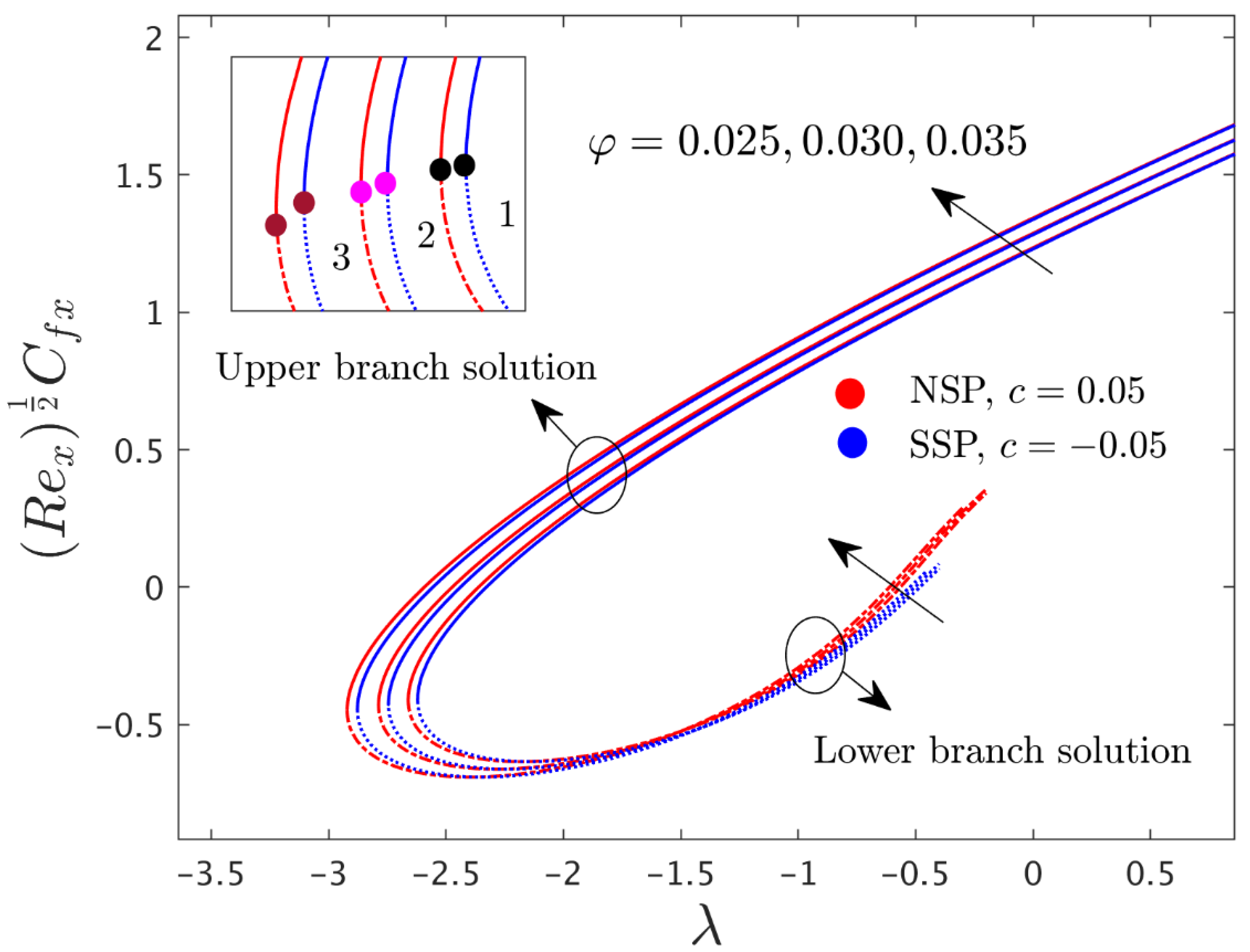
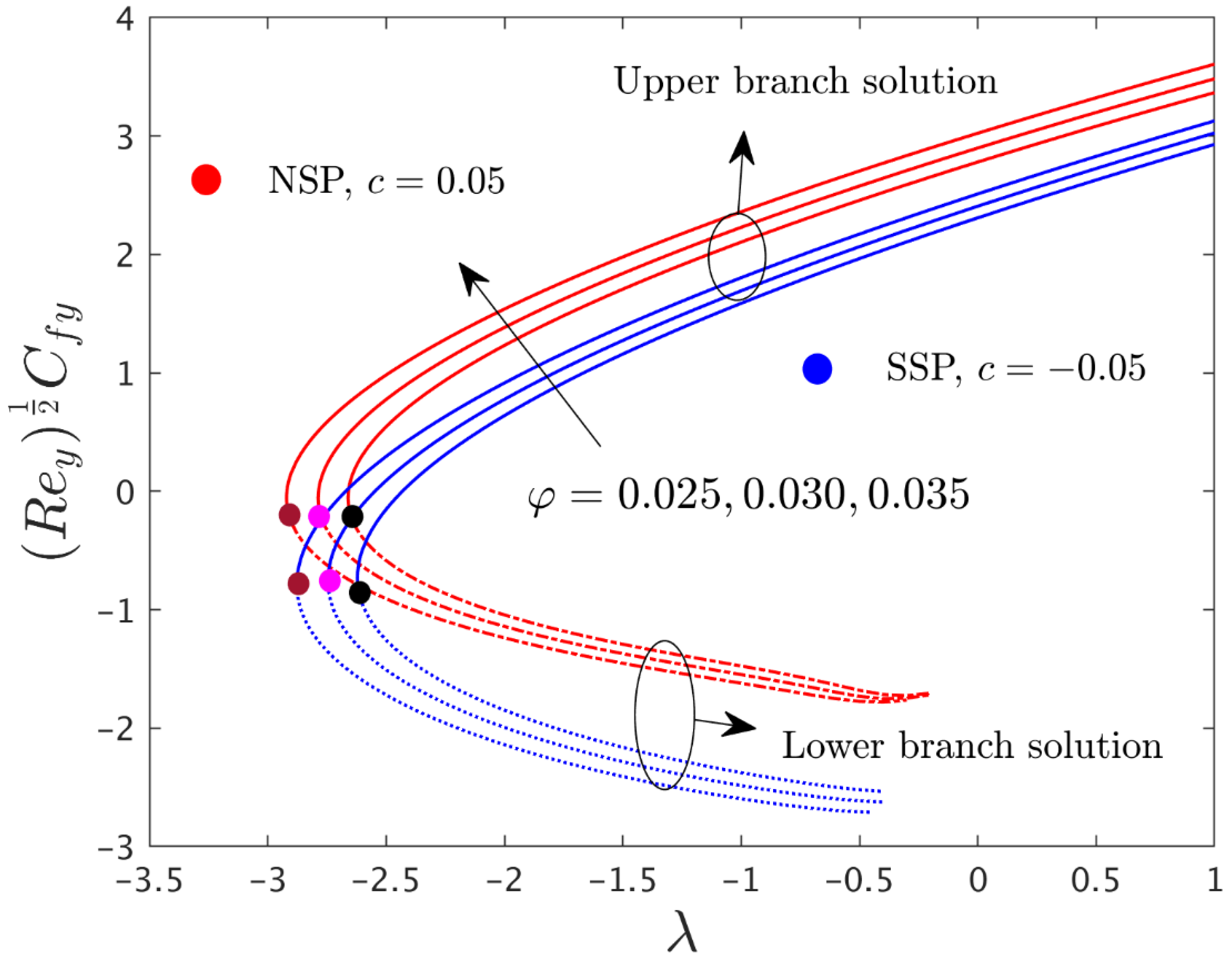
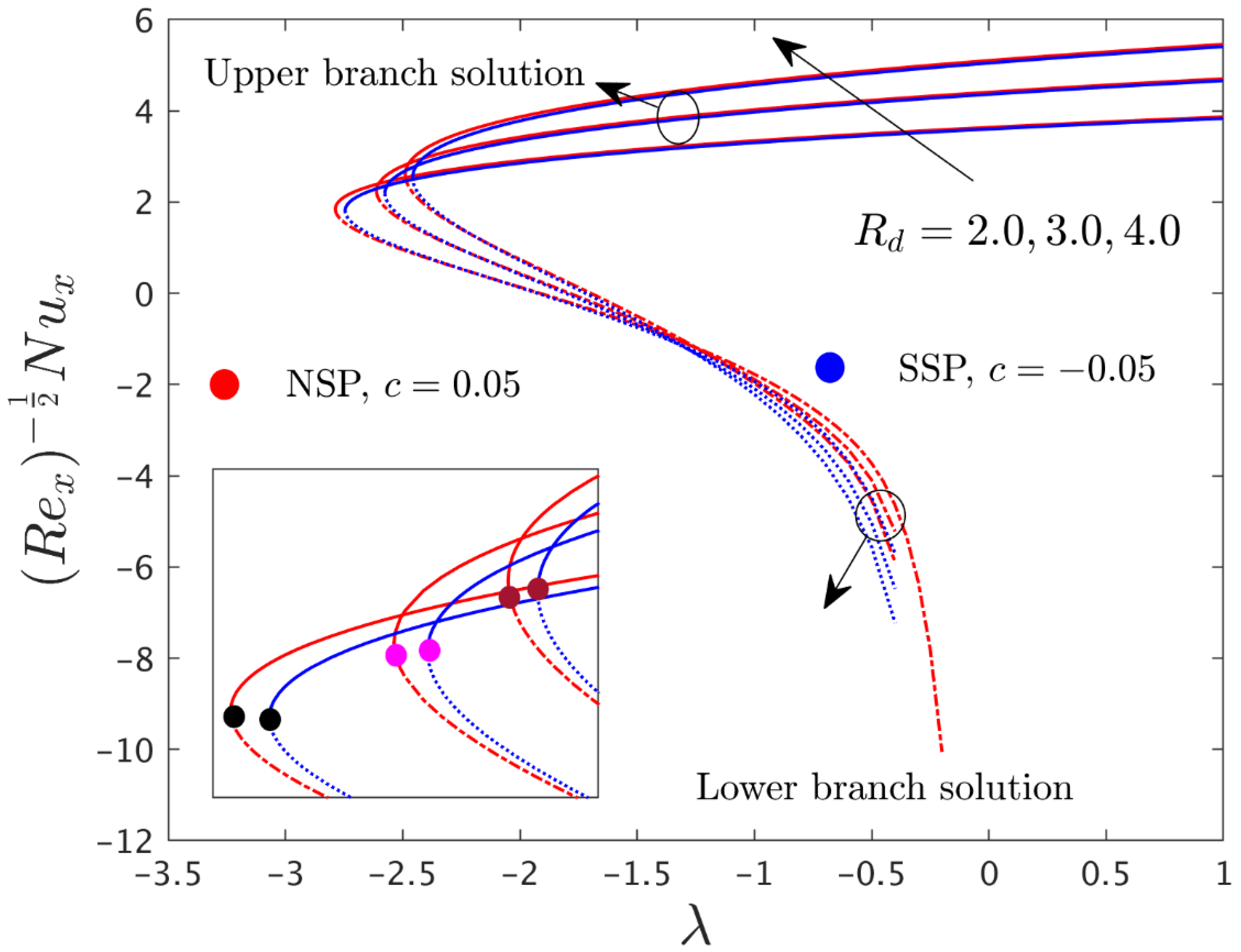
• Upper and lower solution branches in the given research model existed for particular domains of the mixed convection parameter, with impacts from several parameters.
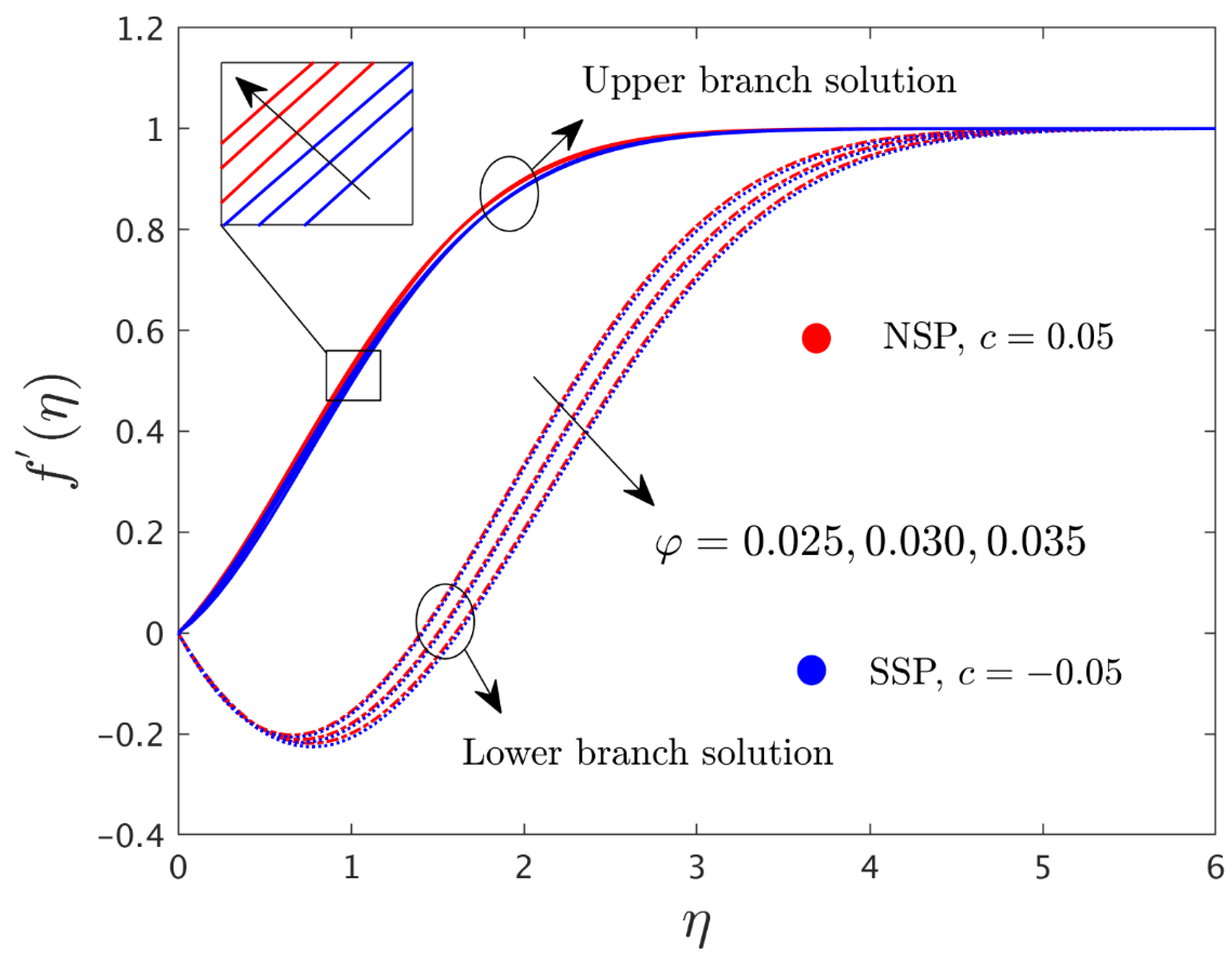
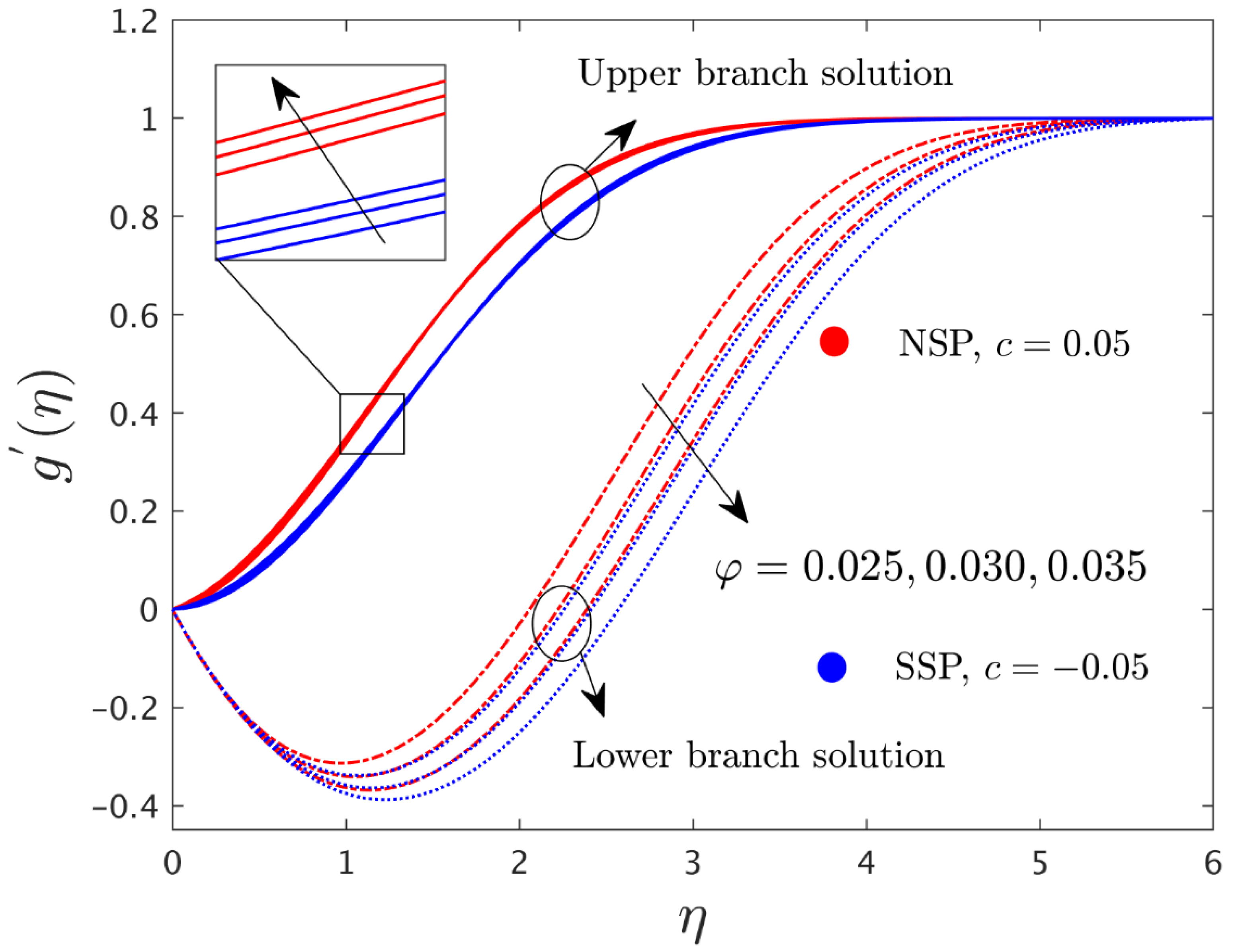
• For higher values of $\phi$, the dimensionless velocity profile in both directions increased for the UBS and decreased for the LBS.
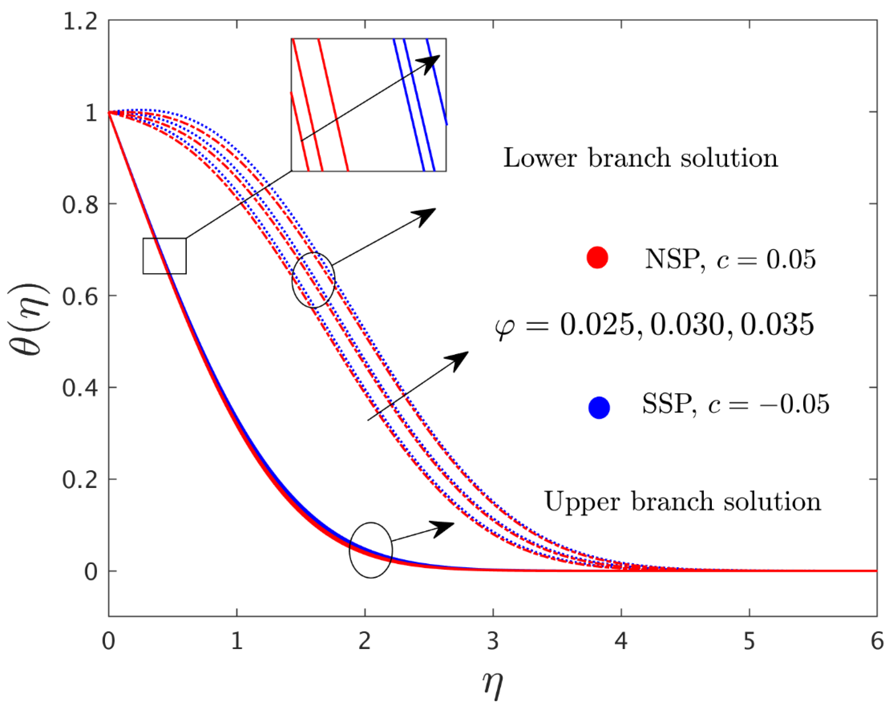
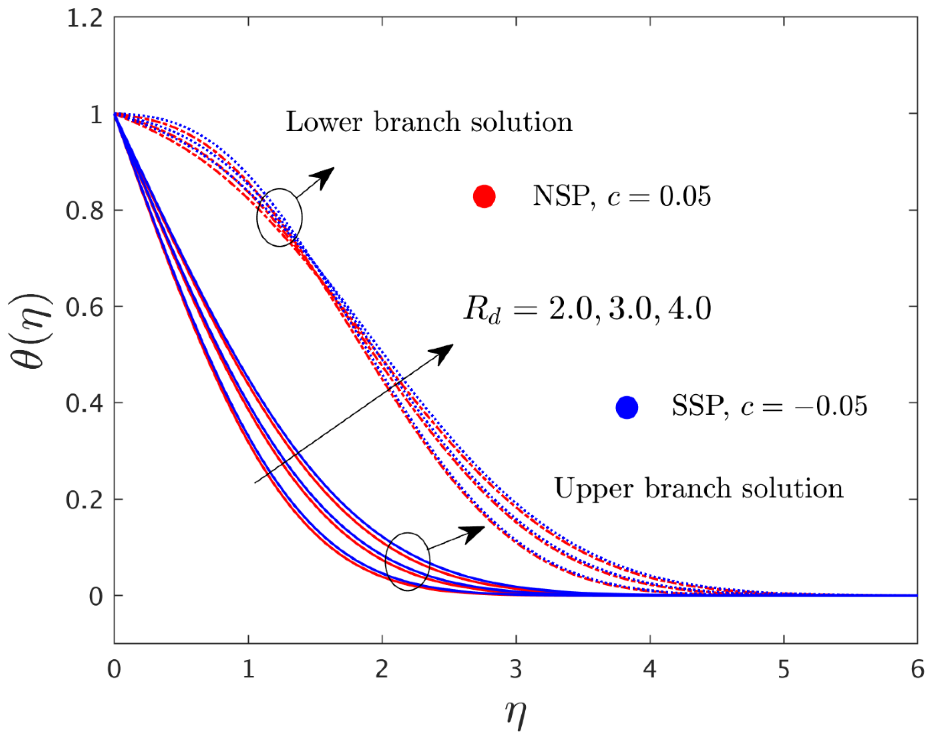
• With a larger consequential value for the radiation parameter and the nanoparticle volume fraction $\phi$, the temperature distribution profile was increased in both solution branches.
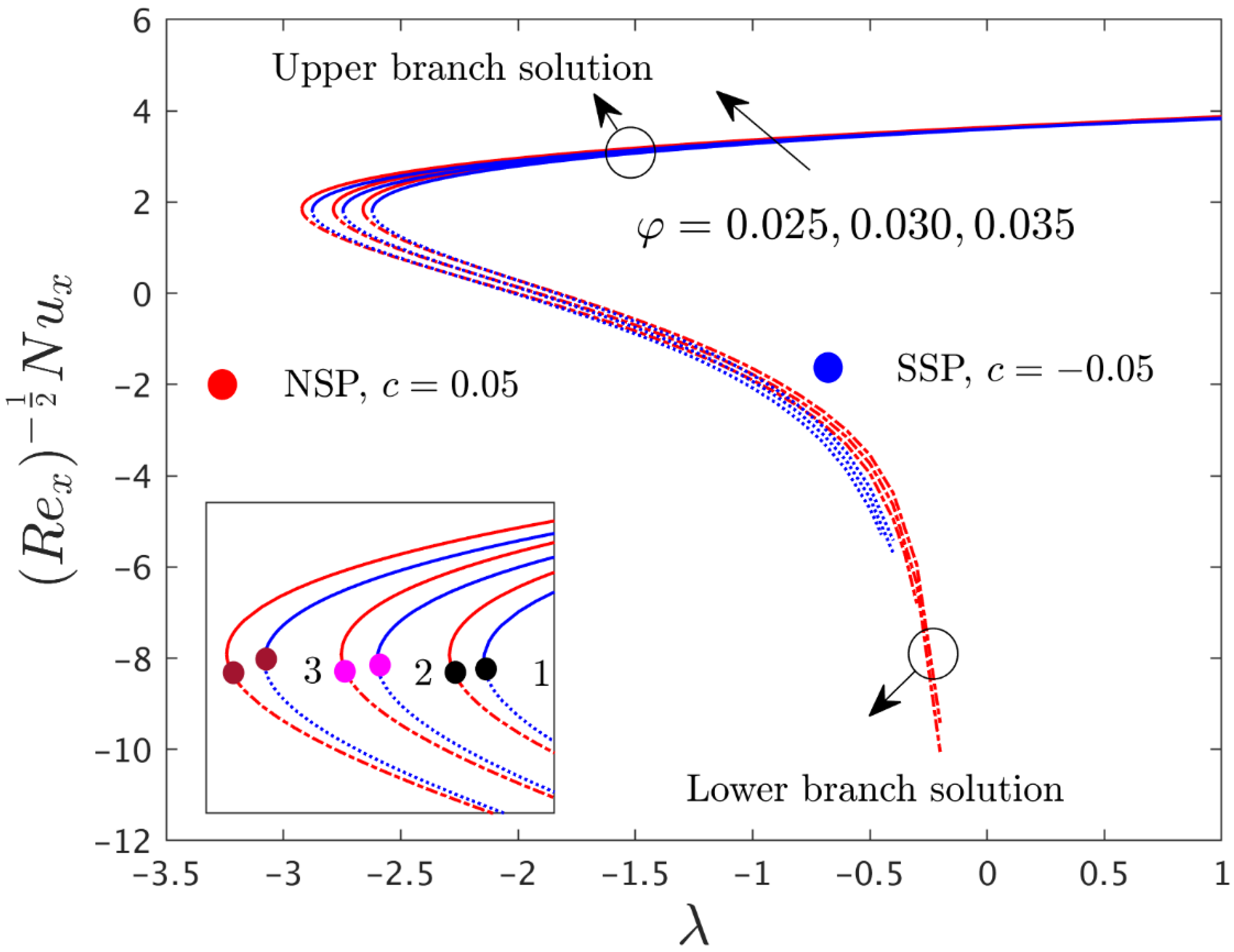
• The magnitude of the critical values increased with $\phi$ and shrank for the larger values of $R_d$.
• The skin friction coefficients in both directions and the rate of heat transfer were augmented with larger values of $\phi$ and $R_d$.
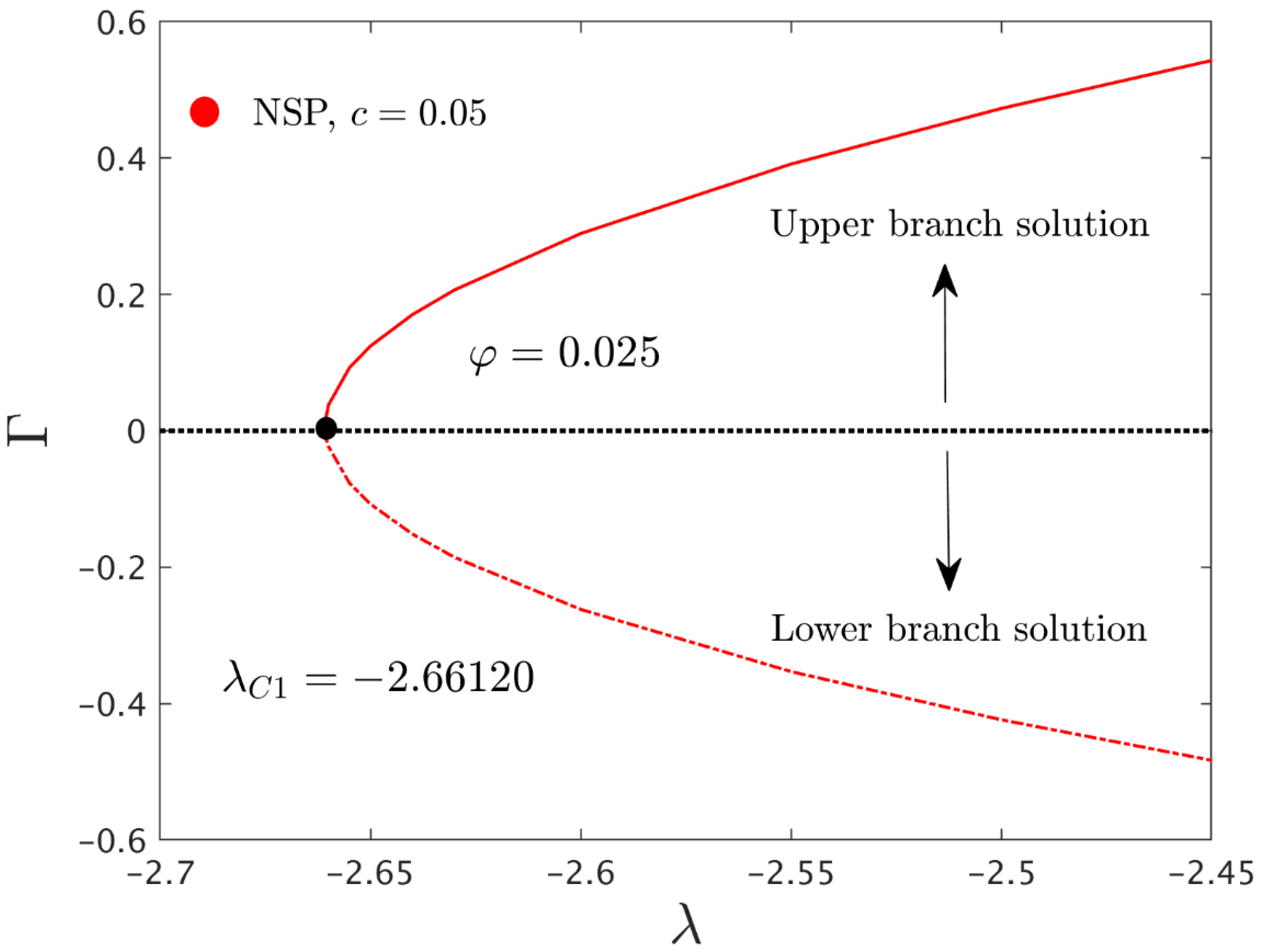
• The stability analysis revealed that the UB solution was stable and physically acceptable while the LB solution was not physically stable.

References

- Choi, S.U.S.; Eastman, J.A. Enhancing Thermal Conductivity of Fluids with Nanoparticles; Technical Report; Argonne National Lab.: Chicago, IL, USA, 1995. [Google Scholar]
- Ellahi, R.; Zeeshan, A.; Vafai, K.; Rahman, H.U. Series solutions for magnetohydrodynamic flow of non-Newtonian nanofluid and heat transfer in coaxial porous cylinder with slip conditions. Proc. Inst. Mech. Eng. Part N J. Nanoeng. Nanosyst. 2011, 225, 123–132. [Google Scholar] [CrossRef]
- Rosmila, A.B.; Kandasamy, R.; Muhaimin, I. Lie symmetry group transformation for MHD natural convection flow of nanofluid over linearly porous stretching sheet in presence of thermal stratification. Appl. Math. Mech. 2012, 33, 593–604. [Google Scholar] [CrossRef]
- Sheikholeslami, M.; Hatami, M.; Ganji, D.D. Analytical investigation of MHD nanofluid flow in a semi-porous channel. Powder Technol. 2013, 246, 327–336. [Google Scholar] [CrossRef]
- Javaherdeh, K.; Ashorynejad, H.R. Magnetic field effects on force convection flow of a nanofluid in a channel partially filled with porous media using Lattice Boltzmann Method. Adv. Powder Technol. 2014, 25, 666–675. [Google Scholar]
- Noor, A.; Nazar, R.; Jafar, K.; Pop, I. Boundary-layer flow and heat transfer of nanofluids over a permeable moving surface in the presence of a coflowing fluid. Adv. Mech. Eng. 2014, 6, 521236. [Google Scholar] [CrossRef]
- Wang, Y.; Su, G.H. Experimental investigation on nanofluid flow boiling heat transfer in a vertical tube under different pressure conditions. Exp. Therm. Fluid. Sci. 2016, 77, 116–123. [Google Scholar] [CrossRef]
- Sandeep, N.; Malvandi, A. Enhanced heat transfer in liquid thin film flow of non-Newtonian nanofluids embedded with graphene nanoparticles. Adv. Powder Technol. 2016, 27, 2448–2456. [Google Scholar] [CrossRef]
- Zuhra, S.; Khan, N.S.; Khan, M.A.; Islam, S.; Khan, W.; Bonyah, E. Flow and heat transfer in water based liquid film fluids dispensed with graphene nanoparticles. Results Phys. 2018, 8, 1143–1157. [Google Scholar] [CrossRef]
- Ghosh, S.; Mukhopadhyay, S. Some Aspects of forced convection nanofluid flow over a moving plate in a porous medium in the presence of heat source/sink. J. Eng. Thermophys. 2019, 28, 291–304. [Google Scholar] [CrossRef]
- Xue, S.; Li, H.; Guo, Y.; Zhang, B.; Li, J.; Zeng, X. Water lubrication of graphene oxide-based materials. Friction 2022, 10, 977–1004. [Google Scholar] [CrossRef]
- Khan, U.; Zaib, A.; Pop, I.; Waini, I.; Ishak, A. MHD flow of a nanofluid due to a nonlinear stretching/shrinking sheet with a convective boundary condition: Tiwari–Das nanofluid model. Int. J. Numer. Methods Heat Fluid Flow 2022. ahead-of-print. [Google Scholar] [CrossRef]
- Ramachandran, N.; Chen, T.S.; Armaly, B.F. Mixed convection in stagnation flows adjacent to vertical surfaces. ASME J. Heat Transf. 1988, 110, 373–377. [Google Scholar] [CrossRef]
- Devi, C.S.; Takhar, H.S.; Nath, G. Unsteady mixed convection flow in stagnation region adjacent to a vertical surface. Heat Mass Transf. 1991, 26, 71–79. [Google Scholar] [CrossRef]
- Bachok, N.; Ishak, A.; Pop, I. Mixed convection boundary layer flow near the stagnation point on a vertical surface embedded in a porous medium with anisotropy effect. Transp. Porous Media 2010, 82, 363–373. [Google Scholar] [CrossRef]
- Bhattacharyya, K.; Mukhopadhyay, S.; Layek, G.C. Similarity solution of mixed convective boundary layer slip flow over a vertical plate. Ain Shams Eng. J. 2013, 4, 299–305. [Google Scholar] [CrossRef]
- Rosali, H.; Ishak, A.; Nazar, R.; Pop, I. Mixed convection boundary layer flow past a vertical cone embedded in a porous medium subjected to a convective boundary condition. Propuls. Power Res. 2016, 5, 118–822. [Google Scholar] [CrossRef]
- Mahat, R.; Rawi, N.A.; Kasim, A.R.; Shafie, S. Heat generation effect on mixed convection flow of viscoelastic nanofluid: Convective boundary condition solution. Malays. J. Fundam. Appl. Sci. 2020, 16, 166–672. [Google Scholar] [CrossRef]
- Khan, A.Q.; Rasheed, A. Mixed convection magnetohydrodynamics flow of a nanofluid with heat transfer: A numerical study. Math. Probl. Eng. 2019, 2019, 8129564. [Google Scholar] [CrossRef]
- Bouslimi, J.; Abdelhafez, M.A.; Abd-Alla, A.M.; Abo-Dahab, S.M.; Mahmoud, K.H. MHD mixed convection nanofluid flow over convectively heated nonlinear due to an extending surface with Soret effect. Complexity 2021, 2021, 5592024. [Google Scholar] [CrossRef]
- Devi, S.U.; Devi, S.A. Heat transfer enhancement of Cu-Al2O3/water hybrid nanofluid flow over a stretching sheet. J. Nigerian Math. Soc. 2017, 36, 419–433. [Google Scholar]
- Chu, Y.; Nisar, K.S.; Khan, U.; Kasmaei, H.D.; Malaver, M.; Zaib, A.; Khan, I. Mixed convection in MHD water-based molybdenum disulfide-Graphene Oxide hybrid nanofluid through an upright cylinder with shape factor. Water 2020, 12, 1723. [Google Scholar] [CrossRef]
- Bataller, R.C. Radiation effects in the Blasius flow. Appl. Math. Comput. 2008, 198, 333–338. [Google Scholar]
- Ishak, A. Thermal boundary layer flow over a stretching sheet in a micropolar fluid with radiation effect. Meccanica 2010, 45, 367–373. [Google Scholar] [CrossRef]
- Magyari, E.; Pantokratoras, A. Note on the effect of thermal radiation in the linearized Rosseland approximation on the heat transfer characteristics of various boundary layer flows. Int. Commun. Heat Mass Transf. 2011, 38, 554–556. [Google Scholar] [CrossRef]
- Merkin, J.H. On dual solutions occurring in mixed convection in a porous medium. J. Eng. Math. 1986, 20, 171–179. [Google Scholar] [CrossRef]
- Weidman, P.D.; Kubitschek, D.G.; Davis, A.M. The effect of transpiration on self-similar boundary layer flow over moving surfaces. Int. J. Eng. Sci. 2006, 44, 730–737. [Google Scholar] [CrossRef]
- Khan, U.; Zaib, A.; Mebarek-Oudina, F. Mixed convective magneto flow of SiO2–MoS2/C2H6O2 hybrid nanoliquids through a vertical stretching/shrinking wedge: Stability analysis. Arab J. Sci. Eng. 2020, 45, 9061–9073. [Google Scholar] [CrossRef]
- Harris, S.D.; Ingham, D.B.; Pop, I. Mixed convection boundary-layer flow near the stagnation point on a vertical surface in a porous medium: Brinkman model with slip. Transp. Porous Media 2009, 77, 267–285. [Google Scholar] [CrossRef]
- Shampine, L.F.; Gladwell, I.; Thompson, S. Solving ODEs with Matlab; Cambridge University Press: Cambridge, UK, 2003. [Google Scholar]
- Dinarvand, S.; Hosseini, R.; Damangir, E.; Pop, I. Series solutions for steady three-dimensional stagnation point flow of a nanofluid past a circular cylinder with sinusoidal radius variation. Meccanica 2013, 48, 643–652. [Google Scholar] [CrossRef]
- Bhattacharyya, S.; Gupta, A.S. MHD flow and heat transfer at a general three-dimensional stagnation point. Int. J. Non Linear Mech. 1998, 33, 125–134. [Google Scholar] [CrossRef]
Publisher’s Note: MDPI stays neutral with regard to jurisdictional claims in published maps and institutional affiliations. |
© 2022 by the authors. Licensee MDPI, Basel, Switzerland. This article is an open access article distributed under the terms and conditions of the Creative Commons Attribution (CC BY) license (https://creativecommons.org/licenses/by/4.0/).