A Parallel Convolution and Decision Fusion-Based Flower Classification Method

Abstract

Flower classification is of great significance to the fields of plants, food, and medicine. However, due to the inherent inter-class similarity and intra-class differences of flowers, it is a difficult task to accurately classify them. To this end, this paper proposes a novel flower classification method that combines enhanced VGG16 (E-VGG16) with decision fusion. Firstly, facing the shortcomings of the VGG16, an enhanced E-VGG16 is proposed. E-VGG16 introduces a parallel convolution block designed in this paper on VGG16 combined with several other optimizations to improve the quality of extracted features. Secondly, considering the limited decision-making ability of a single E-VGG16 variant, parallel convolutional blocks are embedded in different positions of E-VGG16 to obtain multiple E-VGG16 variants. By introducing information entropy to fuse multiple E-VGG16 variants for decision-making, the classification accuracy is further improved. The experimental results on the Oxford Flower102 and Oxford Flower17 public datasets show that the classification accuracy of our method reaches 97.69% and 98.38%, respectively, which significantly outperforms the state-of-the-art methods.

1. Introduction

In the field of plant science, flower classification is a significant and difficult task. At present, flower classification faces the following challenges: (1) there are about 369,000 known flowering species worldwide [1]; (2) flowers may have large inter-class similarities and large intra-class differences, as shown in Figure 1; (3) flower images are vulnerable to natural conditions such as light, background, climate, and other factors. The above challenges make accurate flower classification a difficult task.

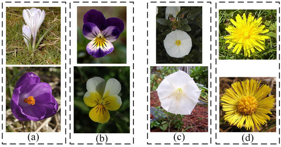
Figure 1. (a) Intra-class differences of crocus. (b) Intra-class differences of pansy. (c) Inter-class similarities between silverbush and thorn apple (the above is silverbush, the below is a thorn apple). (d) Inter-class similarities between dandelion and coltsfoot (the above is dandelion, the below is a coltsfoot).

Extracting representative features is key to accurate flower classification. Traditional flower classification methods use artificially defined features such as color, shape, and texture, which leads to high cost and subjectivity.

Compared with artificial feature extraction, deep learning can be viewed as a self-learning process [2]. Features extracted from deep convolutional neural networks are more representative than features extracted by traditional manual methods. Therefore, applying depth convolutional features to image classification tasks often achieves better results [3]. With the emergence of deep learning models such as AlexNet [4], VGGNet [5], GoogLeNet [6], ResNet [7], and DenseNet [8], many deep learning-based flower classification methods have been proposed. These methods either use a single deep learning model [9,10,11] or combine multiple models [12,13,14], combined with interest region extraction [15,16,17,18], feature selection [12,17], feature combination [9,13,14,19,20] and many other techniques, to improve the quality of extracted features.

However, most existing methods only focus on extracting or selecting effective features, while ignoring the influences of decision-making methods, so their classification accuracies need to be improved.

To this end, this paper proposes a novel enhanced VGG16 model, E-VGG16, which enhances VGG16 by introducing parallel convolution blocks designed in this paper and integrates batch normalization (BN) and global average pooling layers (GAP) for optimization. Additionally, by embedding PCB in different positions of the E-VGG16, multiple high-quality variants are obtained. Based on these variants, information entropy is introduced to exploit the different decision-making capabilities of multiple variants to further improve the classification accuracy.

The main contributions of this paper are as follows:

• This paper designs a simple but effective parallel convolution block (PCB). E-VGG16 is obtained by integrating modules such as PCB and GAP into the VGG16 model, which effectively improves the performance of the model.
• Multiple variants are obtained by embedding PCB in different positions of E-VGG16, and information entropy is introduced to fuse the decisions of multiple variants, thereby further improving the classification accuracy.
• Extensive experiments on Oxford Flower102 and Oxford Flower17 datasets show that the classification accuracy of the proposed method can reach 97.69% and 98.38%, respectively, which significantly outperforms the state-of-the-art algorithms.

The rest of this paper is organized as follows. Section 2 presents related work. Section 3 introduces the E-VGG16 and decision fusion. Section 4 presents the experimental results and analysis. Section 5 concludes the paper.

2. Related Works

2.1. Flower Classification

There are two main ways to extract features: traditional methods and deep learning-based methods.

2.1.1. Traditional Methods

Traditional methods first extract local features such as SIFT (scale invariant feature transform) [21] and HOG (histogram of oriented gradient) [22], then use encoding models such as VLAD (vector of locally aggregated descriptors) [23] or Fisher vector [24,25] to encode features for post-processing. Mabrouk et al. [26] proposed a SURF [27] (speeded up robust features)-based color feature extraction strategy, which describes the visual content of the flower images using compact and accurate descriptors. Kishotha et al. [28] analyzed the influences of multiple local features including shape, texture, color, SIFT, SURF, HSV, RGB and CTM, and found that SURF + CTM presents a better performance than the other feature combinations. Soleimanipour et al. [29] extracted Haar features to train the Viola–Jones detector. This detector was used to detect the spadix region in the test images, and then image templates were used to classify various anthurium flowers.

In general, traditional methods suffer from three main shortcomings [30]: (1) it is hard for them to distinguish the subtle differences between visually similar species; (2) they mainly focus on high-level visual cues, ignoring the importance of low-level visual cues; (3) the feature extraction and final classification are performed independently, which prevents the global optimization of the classification model.

2.1.2. Deep Learning-Based Methods

Considering the shortcomings of traditional methods, in recent years, many studies on flower classification have turned to deep learning based methods. Some deep learning methods first select rough target regions from images, and then use deep learning models for classification [15,16,17,18,31]. Huang et al. [16] proposed a two-stage classification method. In the first stage, a series of polygons are generated, and a classifier is trained for each polygon for rough classification. In the second stage, the confusing classes of the first stage are selected and employed to train the polygon-based classifiers. Wei et al. [17] proposed a selective convolutional descriptor aggregation (SCDA) method, which first discards the background noise in the image and then expresses the retained useful deep descriptors as a feature vector for classification. Hiary et al. [31] proposed a two-stage method, with each stage needs a separate neural network classifier. The first stage crops the region around the flower using a FCN. The second stage uses the cropped images to learn a strong CNN classifier to classify different flowers.

Some other methods directly extract high-quality features from original images by adopting various methods such as feature selection, and feature fusion. Mesut et al. [12] proposed a feature selection and CNN hybrid method, which combines features extracted from four different CNNs, and then chooses the intersecting features of two different feature selection methods. They obtained good accuracy on 5 specific kinds of flowers. Cıbuk et al. [13] proposed a method which uses minimum redundancy maximum correlation (mRMR) to select the most important features etracted from AlexNet and VGG16 and then trained these features with a support-vector machine (SVM).

In addition, unlike methods based on images only, multimodal learning [30,32,33,34,35], which fuses text, images and other modals, has increasingly attracted the attention among researchers in recent years. Based on m-CNN [30], Bae et al. [14] proposed an improved m-CNN, which extracts images and texts features through image CNN and text CNN networks, respectively, and then concatenates these two kinds of features for flower classification.

Different from the above methods, which use multiple different CNNs or multimodal learnings, this paper introduces multiple E-VGG16 variants and fuses the different decision-making capabilities of these variants to boost the accuracy of flower classification.

2.2. VGG16

VGG16 was proposed by the Visual Geometry Group of Oxford University in 2014. VGG16 consists of five convolutional blocks and three fully connected layers. The first two convolutional blocks are composed of two convolutional layers and one pooling layer, and the last three convolutional blocks are composed of three convolutional layers and one pooling layer. In this paper, the authors denote convi as the ith convolution block, convi_j as the jth convolution layer of the ith convolution block, and convi_pool as the pooling layer of the ith convolution block. The numbers of filters in the five convolution blocks are 64, 128, 256, 512, and 512, respectively. The architecture of VGG16 is shown in Figure 2.

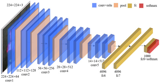
Figure 2. The architecture of VGG16.

The convolution layer filters out the detailed features in the images through a series of convolution operations. During the training process, the parameters of the convolution kernel are continuously updated and optimized through the forward/back propagation process. The pooling layer downsamples features during training, reducing computational complexity. The classifier of VGG16 consists of two fully connected layers with 4096 nodes and one fully connected layer with 1000 nodes, which are finally classified by the softmax function. The authors choose VGG16 as the basic model to research flower classification because it has achieved successful results in the ImageNet challenge and has been widely used in flower classification and many other fields, e.g., A-LDCNN proposed in [36] by integrating VGG16 and Latent Dirichlet Allocation (LDA) [37].

3. The Proposed Method

3.1. E-VGG16

Although VGG16 has good performance in ImageNet and many other applications, it has relatively smaller depth and width compared with some other networks, e.g., GoogLeNet and ResNet; thus, its feature extraction ability and classification effect need to be improved. To this end, this paper presents various optimization methods on VGG16 and then proposes an enhanced VGG16 (E-VGG16). The improvements involved in E-VGG16 mainly include: adding a parallel convolution block (PCB), introducing batch normalization (BN) layers, adding a global average pooling layer (GAP), and adding 1 × 1 convolution.

3.1.1. PCB

Considering the relatively smaller depth and width of VGG16, the most direct way to improve its performance is to increase its network size. In this paper, inspired by GoogLeNet, the authors design a similar parallel convolution block (PCB) on E-VGG16 to expand the network width and increase the network complexity.

The number of parallel convolutional layers k in PCB and the size of convolution kernels are important factors to be considered when designing a PCB. Considering that a larger convolution kernel will bring too many parameters, resulting in the need for dramatically increased computational resources, this paper chooses smaller convolution kernels such as 3 × 3 and 1 × 1, which can keep relatively low computational overheads while expanding the network width. For the number of parallel convolutional layers k, this paper believes that an appropriate k can effectively improve the performance of the network, but too large a k will lead to too many network parameters, thereby reducing performance. The experiments in this paper also confirm this point of view. Based on the experimental comparisons and analyses, this paper adopts four 3 × 3 parallel convolutional layers with 512 filters, one maximum pooling layer and one 1 × 1 convolution layer with 512 filters as our final PCB structure, which is shown in Figure 3.

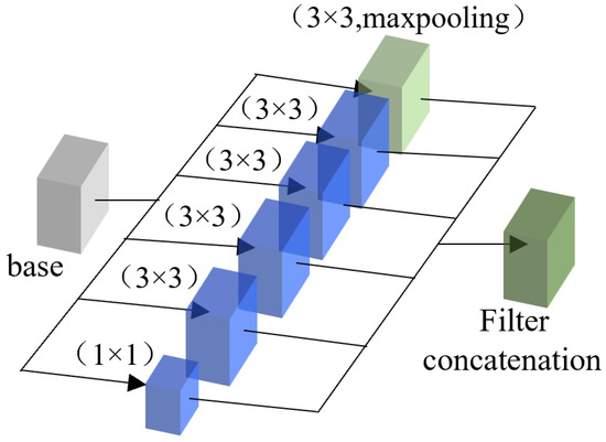
Figure 3. A PCB with k = 4.

The embedded position of PCB in E-VGG16 also has an important impact on network performance. Theoretically, PCB can be embedded within or after one of the five convolutional blocks of VGG16. Depending on the embedded positions of PCB in VGG16, several different E-VGG16 variants can be obtained. After PCB is embedded, the authors remove the remaining part of the convolution block where PCB is embedded and the convolution blocks after the embedding position. For example, if PCB is embedded between conv4_2 and conv4_3, conv4_3, conv4_pool and conv5 will be removed in the network, and the obtained variant will be denoted as $EV4\_2$. Decision fusion will be performed on the obtained variants later to further improve the performance of flower classification.

3.1.2. 1 × 1 Convolutional Layer

Notably, 1 × 1 convolution [38] can realize cross-channel interaction and information integration, reduce the number of parameters and increase nonlinearity while increasing the depth of the network, so it is widely used in GoogLeNet, ResNet, and DenseNet. In this paper, a 1 × 1 convolutional layer is introduced after the PCB to further optimize the model. Since it is the last convolutional layer of E-VGG16, it is denoted as convl hereafter.

3.1.3. BN Layer

The process of training a deep neural network is complicated due to the distribution of each layer’s inputs changes with the parameters of the previous layers during the training process. To alleviate this problem, a small learning rate and careful parameter initialization need to be set, which slows down the training speed. To address this problem, Sergey et al. [39] proposed BN (batch normalization), which normalizes each training mini-batch to a standard normal distribution with mean 0 and variance 1. Given a small batch sample set $B=\{x_1\cdots x_m\}$, whose mean and variance are denoted as $\mu$ and ${\sigma }^2$, respectively, $ϵ$ is a constant to stabilize the data, and the batch data can be standardized by Formula (1):

$${\hat{x}}_i=\frac{x_i-\mu }{\sqrt{{\sigma }^2+ϵ}}$$

(1)

Considering that only using the above normalization formula will affect the features learned, the normalized data are transformed and reconstructed according to Formula (2) to restore the feature distribution to be learned by the original network:

$${\hat{y}}_i=\gamma {\hat{x}}_i+\beta$$

(2)

where $\gamma$ and $\beta$ are learnable reconstruction parameters. BN layers can alleviate the problem of the parameter distribution deviation of the initial value and the intermediate value during the training process. They can also alleviate the problem of gradient disappearance or gradient explosion to a certain extent, thus speeding up the training speed. Although BN layers have been widely used in deep learning-based applications [6,8,40], the number and embedding position of BN layers need to be further discussed [41].

Considering this, this paper introduces three BN embedding points (as the red dots marked in Figure 4): before PCB, between PCB and convl, and after conv l, corresponding to the embedding position p = 0, 1, 2, respectively. According to whether a BN layer is embedded in the pth position, eight different embedding schemes numbered from 0 to 7 are designed. If the pth bit of scheme s is 1, this means a BN layer is embedded in the position corresponding to p; otherwise, vice-versa. For example, scheme 5 (101 in binary) means that two BN layers are embedded before PCB and after convl. The effects of different embedding schemes are verified by experiments to determine the optimal embedding scheme.

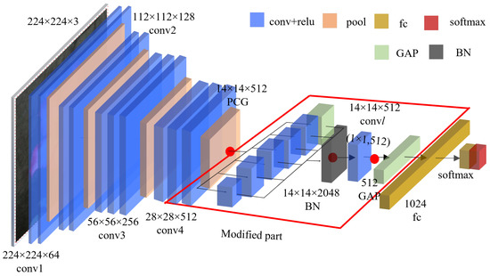
Figure 4. E-VGG16 structure.

3.1.4. GAP Layer

Compared with fully connected layers, a GAP layer has the following merits: (1) it makes the feature map easier to be interpreted as a class confidence map; (2) no parameters are needed to be trained in GAP; thus network training can be speeded up and overfitting can be effectively alleviated; (3) GAP aggregates spatial information, making it more robust to spatial transformations of the inputs [38]. In this paper, the authors replace the first two fully connected layers in VGG16 with a GAP layer, which significantly reduces network parameters and increases training speed.

3.2. Decision Fusion

The softmax classifier in VGG16 always directly outputs the class with the highest probability as the final classification result. This may cause wrong decisions, especially when the probabilities of the other classes are close to the highest probability.

As mentioned earlier, different variants can be obtained according to the positions of PCB embedded in E-VGG16. Different variants have different decision-making abilities. Therefore, multiple variants can be comprehensively used to make the final decision, which can alleviate the problem of classification errors caused by the insufficient decision-making ability of a single variant. To this end, this paper introduces information entropy [42] to evaluate the decision-making certainty of each E-VGG16 variant and then assigns a decision weight to each variant according to the certainty to fuse decision. The E-VGG16-based decision fusion framework is shown in Figure 5.

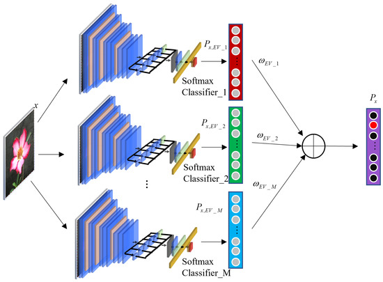
Figure 5. A diagram of decision fusion.

Although multiple variants can be obtained by embedding PCB, it is unrealistic to fuse all E-VGG16 variants because of the following reasons: (1) the computation overhead is large; (2) the classification accuracy will be deteriorated if the variants with poor decision-making abilities are fused. Therefore, this paper evaluates the decision-making ability of each variant in the experimental section and then chooses some best variants for decision-making.

Assuming that there are M E-VGG16 variants involved in decision fusion to classify a sample x, the probability of x belonging to each class can be obtained for each variant, and then the probability distribution vector $P_{x,E{V}_m}$ can be obtained for the mth variant, $E{V}_m$, as shown in Formula (3).

$$P_{x,E{V}_m}=[p_{m1}\left(x\right)p_{m2}\left(x\right)\cdots p_{mC}\left(x\right)]$$

(3)

where $p_{mc}\left(x\right)$ represents the probability that $E{V}_m$ classifies x into the cth class, s.t., $1\le m\le M$, $1\le c\le C$ and C is the total number of classes. In the later description, the authors also denote m as the mth variant and c as the cth class when there is no ambiguity.

To fuse the decisions of multiple variants, the information entropy of the mth variant is calculated according to Formula (4).

$$H_m\left(x\right)=-\sum _{c=1}^C{p}_{mc}\left(x\right){log}_2{p}_{mc}\left(x\right)$$

(4)

$H_m\left(x\right)$ is used to represent the certainty of variant $E{V}_m$ on classifying x. The smaller $H_m\left(x\right)$ of $E{V}_m$ is, the higher the certainty of $E{V}_m$ classifying x will be. A higher decision weight should be assigned to $E{V}_m$. The decision weight of $E{V}_m$ can be calculated according to Formula (5).

$${\omega }_m=\frac{exp(-H_m\left(x\right))}{\sum exp(-H_m\left(x\right))}$$

(5)

In Formula (5), ${\omega }_m$ is calculated using an exponential function, which makes our model more inclined to the variants with higher certainty. After obtaining the decision weight, $p_c\left(x\right)$, the probability of x belonging to class c can be calculated according to Formula (6).

$$p_c\left(x\right)=\frac{{\sum }_{m=1}^M({\omega }_m\times p_{mc}\left(x\right))}{M}$$

(6)

Then, the final probability distribution vector of x $P_x=[p_1\left(x\right)p_2\left(x\right)\cdots p_C\left(x\right)]$ is obtained, where c with the maximum $p_c\left(x\right)$ is the final classification result.

4. Experiments

4.1. Environments

All experiments were carried out on a computer with an Intel i7-7700 CPU @3.6 GHz, 32 GB memory and an NVIDIA GeForce GTX 1060 graphics card running windows 10. Python3.6 was used as the compiler, and Keras was used as the default neural network framework.

The authors conducted experiments on the widely used benchmark datasets Oxford Flower102 [43] and Oxford Flower17 [44]. The former contains 8189 images of 102 kinds of flowers. There are 40 to 258 images of each kind of flower. The latter consists of 17 kinds of flowers with 80 images of each.

In this paper, a cropping method was used to crop a sample image into a square with side length min (w, h) using a selected cropping starting coordinate L in the image, where w and h are the width and height of the original image, respectively. L was determined using Formula (7).

$$L=\left\{\begin{array}{c}(d,0)w\ge h\\ (0,d)w<h\end{array}\right.$$

(7)

where $d=f_{random}\left(|w-h|\right)$ and $f_{random}\left(x\right)$ returns a random value between $[0,x-1]$.

In this paper, the cropping method was executed twice for each image. In this way, each dataset can be enlarged, while the detailed information of the dataset can be fully utilized. The cropped images were scaled to 224 × 224 to be compatible with VGG16 using Lanczos interpolation. Data enhancement was further performed in Keras by random flipping, rotation, and staggered transformations.

The experimental results in this paper were obtained by 5-fold cross-validations. The performances of the proposed model were evaluated by accuracy, sensitivity precision and F1_Score as shown in Formulas (8)–(11), respectively.

$$Acc.=\frac{TP+TN}{TP+TN+FP+FN}$$

(8)

$$Se.=\frac{TP}{TP+FN}$$

(9)

$$Pre.=\frac{TP}{TP+FP}$$

(10)

$$F\_Scr.=\frac{2\times TP}{2\times TP+FP+FN}$$

(11)

where TP, TN, FP and FN stand for true positives, true negatives, false positives, and false negatives, respectively.

4.2. Experiments on Oxford Flower102

4.2.1. Effects of BN Layer

To evaluate the effects of BN on flower classification task, the aforementioned eight BN embedding schemes were compared. In this section, PCB was set as a single convolutional layer with 512 3 × 3 filters, and the embedding point of PCB was set to be conv5_2. The accuracies of different BN embedding schemes are shown in Table 1.

Table 1. Accuracies of different BN embedding schemes.

Schemes	$\mathit{Acc}.(\%)$	$\mathit{Se}.(\%)$	$\mathit{Pre}.(\%)$	$\mathit{F}\_\mathit{Scr}.(\%)$
0	93.97	94.50	93.51	93.53
1	95.55	95.67	95.22	95.21
2	95.66	95.85	94.80	95.33
3	95.42	95.25	95.26	95.05
4	94.33	94.28	93.90	93.73
5	94.91	95.23	95.18	94.87
6	94.60	94.89	94.39	94.32
7	95.18	95.41	94.83	94.85

It can be seen from Table 1 that all evaluation metrics of schemes 1–7 are generally higher than scheme 0 (no embedded BN layer), indicating that embedding BN can effectively improve the accuracy of flower classification. In addition, it can be seen that in schemes 1–7, it is not always true that the more BN layers that are embedded, the better the effects will be. Table 1 shows that scheme 2 is the best among all schemes. The obtained accuracy, sensitivity, precision and F1_Score are 95.66%, 95.85%, 94.80% and 95.33%, respectively. Therefore, in the following experiments, the BN layer is embedded according to scheme 2.

4.2.2. The Effects of PCB

(1)

The effect of the number of parallel convolutional layers k

To investigate the effects of k, the authors designed PCBs containing k = 0 to 5 parallel 3 × 3 convolutional layers, respectively, and experimentally chose the optimal k. Conv5_2 was selected as the default embedding point. The accuracies of different k are shown in Table 2.

Table 2. Accuracies of different k.

k	$\mathit{Acc}.(\%)$	$\mathit{Se}.(\%)$	$\mathit{Pre}.(\%)$	$\mathit{F}\_\mathbf{Scr}.(\%)$
0	88.75	88.87	87.72	87.52
1	96.04	96.04	95.78	95.62
2	96.28	96.37	95.97	95.97
3	96.62	96.62	96.43	96.28
4	96.66	96.85	96.37	96.33
5	96.51	96.73	96.25	96.21

It can be seen from Table 2 that when PCB is not embedded (k = 0), the evaluation scores are 88.75%, 88.87%, 87.72% and 87.52%, respectively, and when k varies from 1 to 5, the evaluation scores can reach more than 95%, which is significantly better than the case without PCB. This shows that PCB plays an important role in improving the classification effect. In addition, all the four evaluation scores increase with the increase in k, and most of them reach their peaks when k = 4. Therefore, the authors use k = 4 as the default value for the subsequent experiments.

(2)

The effects of 1 × 1 convolutional layer and max-pooling layer in PCB

Besides the four parallel 3 × 3 convolutional layers, the effects of adding a 1 × 1 convolutional layer and maximum pooling layer (maxp) in PCB were further investigated. The experimental results are shown in Table 3.

Table 3. Accuracies of 1 × 1 convolutional layer and maximum pooling layer.

k	Layer	$\mathit{Acc}.(\%)$	$\mathit{Se}.(\%)$	$\mathit{Pre}.(\%)$	$\mathit{F}\_\mathit{Scr}.(\%)$
4	-	96.66	96.85	96.37	96.33
	1 × 1	96.13	96.12	95.90	95.74
	maxp	96.74	96.84	96.65	96.53
	all	96.90	97.01	96.70	96.67

In Table 3, “-” means not adding a 1 × 1 convolution layer and maximum pooling layer, and “all” means adding both of them. It can be seen from Table 3 that when k=4, “all” corresponds to the best performance, so the PCB finally designed in this paper contains four parallel 3 × 3 convolutional layers, one 1 × 1 convolutional layer and a maximum pooling layer.

(3)

Effects of embedding positions of PCB

Different layers in E-VGG16 contain different features. The shallower layers in E-VGG16, e.g., conv2 and conv3, contain detailed features such as textures and contours, and the deeper layers e.g., conv4 and conv5, contain more abstract classification features. Different embedding positions of PCB have significant effects on the classification accuracy.

To explore the effects of embedding positions of PCB, multiple embedding positions were adopted, resulting in multiple different E-VGG16 variants. Considering that the first three convolutional blocks at the shallower layers mainly contain detailed features, the corresponding pooling layers were selected as the embedding positions. and 3 embedding points were obtained: conv1-pool, conv2-pool, and conv3-pool. For the deeper convolution blocks containing rich classification information, all layers in these blocks including conv4-1, conv4-2, conv4-3, conv4-pool, conv5-1. conv5-2, conv5-3, and conv5-pool were selected as the embedding positions. The accuracies of the 11 embedding positions are shown in Figure 6.

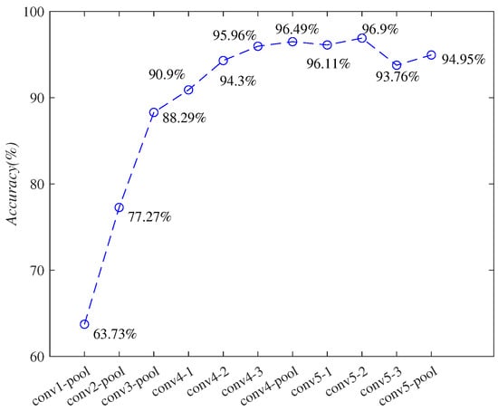
Figure 6. Comparisons corresponding to different PCB embedding positions.

It can be seen from Figure 6 that the embedding positions of PCB have an important impact on the classification accuracy. As the PCB embedding depth increases, the accuracy first increases and then decreases, and reaches the highest 96.90% when embedding position is conv5_2 (denoted as $E{V}_{5\_2}$).The overall accuracies are poor when PCB is embedded in conv1, conv2 and conv3, as they contain less classification information. When PCB is embedded in conv4 and conv5, better results can be obtained, and all accuracies are above 90%.

The accuracy and loss curves of the training and validation for $E{V}_{5\_2}$ are depicted in Figure 7 and Figure 8, respectively. It can be seen from the two figures that when the epoch is 10, the accuracy and loss of the training set reaches 96.89% and 0.14, respectively, which shows E-VGG16 has a quick convergence ability.

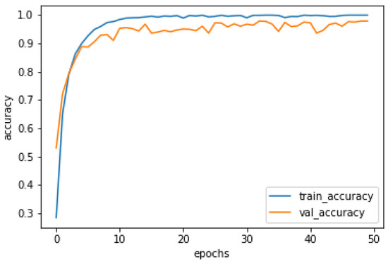
Figure 7. The accuracy curves of the training and validation for $E{V}_{5\_2}$.

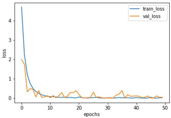
Figure 8. The loss curves of the training and validation for $E{V}_{5\_2}$.

4.2.3. The Effects of Decision Fusion

To evaluate the effectiveness of decision fusion, the three best variants corresponding to the embedding points conv4-pool, conv5-1, and conv5-2 were selected. These three variants are denoted as $E{V}_{4\_p}$, $E{V}_{5\_1}$ and $E{V}_{5\_2}$, respectively. In this paper, experiments on the combinations of these three variants were carried out, and the classification accuracies are shown in Table 4.

Table 4. Classification accuracies on fusing the three best variants.

Schemes	Combinations	$\mathit{Acc}.(\%)$	$\mathit{Se}.(\%)$	$\mathit{Pre}.(\%)$	$\mathit{F}\_\mathit{Scr}.(\%)$
1	$E{V}_{4\_p}$	96.49	95.74	96.01	95.94
2	$E{V}_{5\_1}$	96.11	96.27	95.83	95.74
3	$E{V}_{5\_2}$	96.90	97.01	96.70	96.67
4	$E{V}_{4\_p}$+$E{V}_{5\_1}$	97.11	97.37	97.28	97.14
5	$E{V}_{4\_p}$ + $E{V}_{5\_2}$	97.23	97.32	97.12	97.03
6	$E{V}_{5\_1}$ + $E{V}_{5\_2}$	97.57	97.75	97.39	97.40
7	$E{V}_{4\_p}$ + $E{V}_{5\_1}$ + $E{V}_{5\_2}$	97.69	97.74	97.82	97.65

It can be seen from Table 4 that the effects of fusing multiple variants are generally better than using a single variant. The accuracy of the fusing two variants can reach up to 97.57% ($E{V}_{5\_1}$ + $E{V}_{5\_2}$ ), which is 0.67% higher than the highest single variant model ($E{V}_{5\_2}$). When all the three variants are fused, its accuracy reaches 97.69%, which is 0.79% higher than that of $E{V}_{5\_2}$, which demonstrates the effectiveness of our decision fusion strategy in this paper.

4.2.4. Comparison with the State-of-the-Art Methods

Finally, the proposed methods were compared with the state-of-the-art methods on Oxford Flower102, and the results are shown in Table 5.

Table 5. Comparisons with the state-of-the-art methods on Oxford Flower102.

Method	Years	$\mathit{Acc}.(\%)$
VGG16	2014	91.05
Azizpouret al. [45]	2015	91.3
Yoo et al. [46]	2015	91.28
Simon et al. [10]	2015	95.3
Xu et al. [47]	2016	93.51
Zheng et al. [19]	2016	95.6
Wei et al. [17]	2016	92.1
Liu et al. [15]	2017	84.02
Xia et al. [48]	2017	94.0
Xie et al. [11]	2017	94.01
Chakraborti et al. [49]	2017	94.8
Huang et al. [16]	2017	96.1
Hiary et al. [31]	2018	97.1
Cıbuk et al. [13]	2019	95.70
Bae et al. [14]	2020	93.69
Pang et al. [9]	2020	94.2
E-VGG16(ours)	2022	96.90
E-VGG16 + decision fusion (ours)	2022	97.69

It can be seen from Table 5 that E-VGG16+decision fusion has the highest classification accuracy compared with the others. The accuracy of a single E-VGG16 variant ($E{V}_{5\_2}$) in this paper is up to 96.90% and is 5.85% higher than VGG16, which shows the effectiveness of PCB and the other optimization strategies we used. E-VGG16 is better than all other algorithms except the method proposed by Hiary et al. [31] (Hiary’s), indicating that our E-VGG16 can effectively extract high-quality features. Other than the methods proposed in this paper, the methods proposed by Hiary et al. [31] and Huang et al. [16] are the two with the highest accuracies. Both these two methods adopt two-stage strategies to improve their accuracies and their corresponding accuracies reach 97.1% and 96.1%, respectively. In addition, although the recent work of Bae et al. [14] fused two modalities of image and text, its optimization for each modality is insufficient, so its classification accuracy needs to be improved. Our accuracy can further reach 97.69% by combining information entropy-based decision fusion, which is significantly better than the other competitors.

4.3. Experiments on Oxford Flower17

Experiments were also conducted on Oxford Flower17 using the same experimental settings as those on Oxford Flower102. Differently, on Oxford Flower17, $E{V}_{5\_1}$ is the best single variant with an accuracy of 97.21%, and the combination of $E{V}_{5\_1}$ and $E{V}_{5\_2}$ reaches the best accuracy at 98.38%. The comparisons of our method with the state-of-the-art methods on Oxford Flower17 are shown in Table 6.

Table 6. Comparisons with the state-of-the-art methods on Oxford Flower17.

Method	Years	$\mathit{Acc}.(\%)$
VGG16	2014	92.36
Zhu et al. [50]	2015	91.9
Xie et al. [51]	2015	94.8
Zhang et al. [52]	2016	93.7
Zhang et al. [53]	2017	87.1
Xia et al. [48]	2017	95.0
Hiary et al. [31]	2018	98.5
Cıbuk et al. [13]	2019	96.17
Liu et al. [18]	2021	97.35
E-VGG16 (ours)	2022	97.21
E-VGG16 + decision fusion (ours)	2022	98.38

In Table 6, the accuracies of Liu et al. [18] and Hiary et al. [31] on Oxford Flower17 are 97.35% and 98.5%, respectively, which are higher than 97.21%, the accuracy of our single E-VGG16 variant ($E{V}_{5\_1}$). After using decision fusion, The accuracy of our method reaches 98.38%, which is much better than Liu’s method and is comparable to Hiary’s, indicating the effectiveness of the proposed method in this paper. Hiary’s method is the highest among all the methods. The cropped images may play an important role in Hiary’s method, and combining their cropped images with our method will be left as our future work.

5. Conclusions

This paper proposes E-VGG16, which enhances VGG16 and can effectively extract flower features. By embedding PCB into different locations of E-VGG16, multiple high-quality E-VGG16 variants can be obtained. The accuracy of flower classification is further improved by combining information entropy for decision fusion. In the future, the authors will continue to optimize our model. Additionally, introducing text into our model is also an interesting direction.

References

- UK, Royal Botanic Gardens. State of the World’s Plants Report-2016; Royal Botanic Gardens: Richmond, UK, 2016. [Google Scholar]
- Yann, L.C.; Bengio, Y.; Hinton, G. Deep learning. Nature 2015, 521, 436–444. [Google Scholar]
- Donahue, J.; Jia, Y.Q.; Vinyals, O.; Hoffman, J. Decaf: A deep convolutional activation feature for generic visual recognition. In Proceedings of the International Conference on Machine Learning, Beijing, China, 21–26 June 2014. [Google Scholar]
- Krizhevsky, A.; Sutskever, I.; Hinton, G. Imagenet classification with deep convolutional neural networks. Adv. Neural Inf. Process. Syst. 2012, 25, 142–149. [Google Scholar] [CrossRef]
- Simonyan, K.; Zisserman, A. Very deep convolutional networks for large-scale image recognition. arXiv 2014, arXiv:1409.1556. [Google Scholar]
- Szegedy, C.; Liu, W.; Jia, Y.Q.; Sermanet, P. Going deeper with convolutions. In Proceedings of the IEEE Conference on Computer Vision and Pattern Recognition, Boston, MA, USA, 7–12 June 2015. [Google Scholar]
- He, K.M.; Zhang, X.Y.; Ren, S.Q.; Sun, J. Deep residual learning for image recognition. In Proceedings of the IEEE Conference on Computer Vision and Pattern Recognition, Las Vegas, NV, USA, 27–30 June 2016. [Google Scholar]
- Huang, G.; Liu, Z.; Van, D.; Weinberger, K. Densely connected convolutional networks. In Proceedings of the IEEE Conference on Computer Vision and Pattern Recognition, Honolulu, HI, USA, 21–26 July 2017. [Google Scholar]
- Pang, C.; Wang, W.H.; Lan, R.S.; Shi, Z. Bilinear pyramid network for flower species categorization. Multimed. Tools Appl. 2021, 80, 215–225. [Google Scholar] [CrossRef]
- Simon, M.; Rodner, E. Neural activation constellations: Unsupervised part model discovery with convolutional networks. In Proceedings of the IEEE International Conference on Computer Vision, Santiago, Chile, 7–13 December 2015. [Google Scholar]
- Xie, L.x.; Wang, J.D.; Lin, W.Y.; Zhang, B. Towards reversal-invariant image representation. Int. J. Comput. Vis. 2017, 123, 226–250. [Google Scholar] [CrossRef]
- Toğaçar, M.; Ergen, B.; Cömert, Z. Classification of flower species by using features extracted from the intersection of feature selection methods in convolutional neural network models. Measurement 2020, 158, 107703. [Google Scholar] [CrossRef]
- Cıbuk, M.; Budak, U.; Guo, Y.H.; Ince, M. Efficient deep features selections and classification for flower species recognition. Measurement 2019, 137, 7–13. [Google Scholar] [CrossRef]
- Bae, K.I.; Park, J. Flower classification with modified multimodal convolutional neural networks. Expert Syst. Appl. 2020, 159, 113455. [Google Scholar] [CrossRef]
- Liu, Y.Y.; Tang, F.; Zhou, D.W.; Meng, Y.P. Flower classification via convolutional neural network. In Proceedings of the 2016 IEEE International Conference on Functional-Structural Plant Growth Modeling, Simulation, Visualization and Applications (FSPMA), Qingdao, China, 7–11 November 2016. [Google Scholar]
- Huang, C.; Li, H.L.; Xie, Y.R.; Wu, Q.B.; Luo, B. PBC: Polygon-based classifier for fine-grained categorization. IEEE Trans. Multimed. 2016, 19, 673–684. [Google Scholar] [CrossRef]
- Wei, X.S.; Luo, J.H.; Wu, J.X.; Zhou, Z.H. Selective convolutional descriptor aggregation for fine-grained image retrieval. IEEE Trans. Image Process. 2017, 26, 2868–2881. [Google Scholar] [CrossRef] [PubMed] [Green Version]
- Liu, C.; Huang, L.; Wei, Z.Q.; Zhang, W.F. Subtler mixed attention network on fine-grained image classification. Appl. Intell. 2021, 51, 7903–7916. [Google Scholar] [CrossRef]
- Zheng, L.; Zhao, Y.; Wang, S.; Wang, J.; Tian, Q. Good practice in CNN feature transfer. arXiv 2016, arXiv:1604.00133. [Google Scholar]
- Ahmed, K.T.; Irtaza, A.; Iqbal, M.A. Fusion of local and global features for effective image extraction. Appl. Intell. 2017, 47, 526–543. [Google Scholar] [CrossRef]
- Lowe, D.G. Distinctive image features from scale-invariant keypoints. Int. J. Comput. Vis. 2004, 60, 91–110. [Google Scholar] [CrossRef]
- Dalal, N.; Triggs, B. Histograms of oriented gradients for human detection. In Proceedings of the 2005 IEEE Computer Society Conference on Computer Vision and Pattern Recognition (CVPR’05), San Diego, CA, USA, 20–25 June 2005. [Google Scholar]
- Jégou, H.; Douze, M.; Schmid, C.; Pérez, P. Aggregating local descriptors into a compact image representation. In Proceedings of the 2010 IEEE Computer Society Conference on Computer Vision and Pattern Recognition, San Francisco, CA, USA, 13–18 June 2010. [Google Scholar]
- Peng, X.J.; Zou, C.Q.; Qiao, Y.; Peng, Q. Action recognition with stacked fisher vectors. In Proceedings of the European Conference on Computer Vision, Zurich, Switzerland, 6–12 September 2014. [Google Scholar]
- Sánchez, J.; Perronnin, F.; Mensink, T.; Verbeek, J. Image classification with the fisher vector: Theory and practice. Int. J. Comput. Vis. 2013, 105, 222–245. [Google Scholar] [CrossRef]
- Mabrouk, A.B.; Najjar, A.; Zagrouba, E. Image flower recognition based on a new method for color feature extraction. In Proceedings of the 2014 International Conference on Computer Vision Theory and Applications (VISAPP), Lisbon, Portugal, 5–8 January 2014. [Google Scholar]
- Bay, H.; Tuytelaars, T.; Gool, L.V. Surf: Speeded up robust features. In Proceedings of the European Conference on Computer Vision, Graz, Austria, 7–13 May 2006. [Google Scholar]
- Kishotha, S.; Mayurathan, B. Machine learning approach to improve flower classification using multiple feature set. In Proceedings of the 2019 14th Conference on Industrial and Information Systems (ICIIS), Kandy, Sri Lanka, 18–20 December 2019. [Google Scholar]
- Soleimanipour, A.; Chegini, G.R. A vision-based hybrid approach for identification of Anthurium flower cultivars. Comput. Electron. Agric. 2020, 174, 105460. [Google Scholar] [CrossRef]
- Abdelghafour, F.; Rosu, R.; Keresztes, B.; Germain, C.; Da, C.J. A Bayesian framework for joint structure and colour based pixel-wise classification of grapevine proximal images. Comput. Electron. Agric. 2019, 158, 345–357. [Google Scholar] [CrossRef]
- Hiary, H.; Saadeh, H.; Saadeh, M.; Yaqub, M. Flower classification using deep convolutional neural networks. IET Comput. Vis. 2018, 12, 855–862. [Google Scholar] [CrossRef]
- Tang, J.H.; Li, Z.C.; Lai, H.J.; Zhang, L.Y.; Yan, S.C. Personalized age progression with bi-level aging dictionary learning. IEEE Trans. Pattern Anal. Mach. Intell. 2017, 40, 905–917. [Google Scholar]
- Xu, K.; Ba, J.; Kiros, R.; Cho, K. Show, Attend and Tell: Neural Image Caption Generation with Visual Attention. Comput. Sci. 2015, 37, 2048–2057. [Google Scholar]
- Antol, S.; Agrawal, A.; Lu, J. Vqa: Visual question answering. In Proceedings of the IEEE International Conference on Computer Vision, Santiago, Chile, 7–13 December 2015. [Google Scholar]
- Shu, X.B.; Qi, G.J.; Tang, J.H.; Wang, J.D. Weakly-shared deep transfer networks for heterogeneous-domain knowledge propagation. In Proceedings of the 23rd ACM International Conference on Multimedia, Brisbane, Australia, 26–30 October 2015. [Google Scholar]
- Qin, M.; Xi, Y.H.; Jiang, F. A new improved convolutional neural network flower image recognition model. In Proceedings of the 2019 IEEE Symposium Series on Computational Intelligence (SSCI), Xiamen, China, 6–9 December 2019. [Google Scholar]
- Jia, L.Y.; Tang, J.L.; Li, M.J.; You, J.G.; Ding, J.M.; Chen, Y.N. TWE-WSD: An effective topical word embedding based word sense disambiguation. CAAI Trans. Intell. Technol. 2021, 6, 72–79. [Google Scholar] [CrossRef]
- Lin, M.; Chen, Q.; Yan, S.C. Network in network. arXiv 2013, arXiv:1312.4400. [Google Scholar]
- Ioffe, S.; Szegedy, C. Batch normalization: Accelerating deep network training by reducing internal covariate shift. In Proceedings of the International Conference on Machine Learning, Lille, France, 7–9 July 2015. [Google Scholar]
- Howard, A.G.; Zhu, M.L.; Chen, B. Mobilenets: Efficient convolutional neural networks for mobile vision applications. arXiv 2017, arXiv:1704.04861. [Google Scholar]
- Kohlhepp, B. Deep learning for computer vision with Python. Comput. Rev. 2020, 61, 9–10. [Google Scholar]
- Chen, W.C.; Liu, W.B.; Li, K.Y.; Wang, P.; Zhu, H.X.; Zhang, Y.Y.; Hang, C. Rail crack recognition based on adaptive weighting multi-classifier fusion decision. Measurement 2018, 123, 102–114. [Google Scholar] [CrossRef]
- Nilsback, M.; Zisserman, A. Automated flower classification over a large number of classes. In Proceedings of the 2008 Sixth Indian Conference on Computer Vision, Graphics & Image Processing, Washington, DC, USA, 16–19 December 2008. [Google Scholar]
- Nilsback, M.E.; Zisserman, A. A visual vocabulary for flower classification. In Proceedings of the 2006 IEEE Computer Society Conference on Computer Vision and Pattern Recognition (CVPR’06), New York, NY, USA, 17–22 June 2006. [Google Scholar]
- Azizpour, H.; Razavian, A.S.; Sullivan, J.; Maki, A.; Carlsson, S. From generic to specific deep representations for visual recognition. In Proceedings of the IEEE Conference on Computer Vision and Pattern Recognition Workshops, Boston, MA, USA, 7–12 June 2015. [Google Scholar]
- Yoo, D.; Park, S.; Lee, J. Multi-scale pyramid pooling for deep convolutional representation. In Proceedings of the IEEE Conference on Computer Vision and Pattern Recognition Workshops, Boston, MA, USA, 7–12 June 2015. [Google Scholar]
- Xu, Y.; Zhang, Q.; Wang, L. Metric forests based on Gaussian mixture model for visual image classification. Soft Comput. 2018, 22, 499–509. [Google Scholar] [CrossRef]
- Xia, X.L.; Xu, C.; Nan, B. Inception-v3 for flower classification. In Proceedings of the 2017 2nd International Conference on Image, Vision and Computing (ICIVC), Chengdu, China, 2–4 June 2017. [Google Scholar]
- Chakraborti, T.; McCane, B.; Mills, S.; Pal, U. Collaborative representation based fine-grained species recognition. In Proceedings of the 2016 International Conference on Image and Vision Computing New Zealand (IVCNZ), Palmerston North, New Zealand, 21–22 November 2016. [Google Scholar]
- Zhu, J.; Yu, J.; Wang, C.; Li, F.Z. Object recognition via contextual color attention. J. Vis. Commun. Image Represent. 2015, 27, 44–56. [Google Scholar] [CrossRef]
- Xie, G.S.; Zhang, X.Y.; Shu, X.B.; Yan, S.C.; Liu, C.L. Task-driven feature pooling for image classification. In Proceedings of the IEEE International Conference on Computer Vision, Santiago, Chile, 7–13 December 2015. [Google Scholar]
- Zhang, C.J.; Huang, Q.M.; Tian, Q. Contextual exemplar classifier-based image representation for classification. IEEE Trans. Circuits Syst. Video Technol. 2016, 27, 1691–1699. [Google Scholar] [CrossRef]
- Zhang, C.J.; Li, R.Y.; Huang, Q.M.; Tian, Q. Hierarchical deep semantic representation for visual categorization. Neurocomputing 2017, 257, 88–96. [Google Scholar] [CrossRef]
Publisher’s Note: MDPI stays neutral with regard to jurisdictional claims in published maps and institutional affiliations. |
© 2022 by the authors. Licensee MDPI, Basel, Switzerland. This article is an open access article distributed under the terms and conditions of the Creative Commons Attribution (CC BY) license (https://creativecommons.org/licenses/by/4.0/).