A New Software-Based Optimization Technique for Embedded Latency Improvement of a Constrained MIMO MPC

Abstract

Embedded controllers for multivariable processes have become a powerful tool in industrial implementations. Here, the Model Predictive Control offers higher performances than standard control methods. However, they face low computational resources, which reduces their processing capabilities. Based on pipelining concept, this paper presents a new embedded software-based implementation for a constrained Multi-Input-Multi-Output predictive control algorithm. The main goal of this work focuses on improving the timing performance and the resource usage of the control algorithm. Therefore, a profiling study of the baseline algorithm is developed, and the performance bottlenecks are identified. The functionality and effectiveness of the proposed implementation are validated in the NI myRIO 1900 platform using the simulation of a jet transport aircraft during cruise flight and a tape transport system. Numerical results for the study cases show that the latency and the processor usage are substantially reduced compared with the baseline algorithm, $4.6\times$ and $3.17\times$ respectively. Thus, efficient program execution is obtained which makes the proposed software-based implementation mainly suitable for embedded control systems.

1. Introduction

Most industrial processes are multivariable systems which often present strong interactions between the manipulated and the controlled variables. Here, the definition of a suitable control structure to regulate the system is not often trivial [1], especially when dealing with multiple-objective problems and dynamics complexity. In this scenario, even though diverse strategies are possible [2], Model Predictive Control (MPC) turned out to be among the most effective ones in fulfilling the aforementioned tasks [3,4,5]. Studies found in the recent literature exploit algorithms based on MPC methods applied to several process, in which online optimization problems are involved [6,7,8,9,10]. However, it is well known that MPC is more challenging than other control strategies [11,12]. The challenges and differences arise from the following main aspects:

• The control action must be calculated in a receding horizon manner. MPC solves an optimal control problem at each sampling instant, where a sequence of control moves are optimized and only the first control move is injected into the system [13]. This process is repeated, which translate into a greater computational demand on control platforms [14].
• MPC has been known as powerful tool to deal with system constraints [15].This control strategy addresses the state constraints and input saturations to obtain the manipulation that minimizes the proposed cost funcion [16]. Here, heavy execution load and communication resources are needed [17].
• Use of weighting matrices in the cost function. In MPC approaches the value of the pondering matrices are set a priori, to penalize the large excursion of the tracking error and the deviation of the manipulation. This, to obtain the control action; thus, the optimization process that derives the best results can not usually sustain a low stable computation time [18].

Henceforth, these aspects limits the algorithms that can be used to solve the MPC strategy and has motivated the search for computationally efficient optimization algorithms for practical applications where the sampling period tends to be short [12]. In addition, embedded systems are a powerful tool in industrial implementations. In contrast to personal computer applications, they address low computational resources, but provides portability, low cost and low jitter because of the reduction of software interruptions from the operative systems. Thus; MPC is desirable for embedded applications with fast control cycles, such as bioengineering, aerospace, automotive, etc. These embedded applications require small and power-efficient controllers, capable to solve optimization problems at high sampling rates [19]. The first embedded implementation of an MPC algorithm is reported in [20], which consists of a constrained control strategy for a single-input single-output (SISO) system on a Field-Programmable Gate Array (FPGA). Nowadays, research efforts are focused on the development of embedded MPC implementations with low latency. Nevertheless, the computation complexity makes the multivariable MPC poorly efficient for high speed applications where the controller iteration must be executed in a few milliseconds or even in microseconds.

For this reason, recent research works address the computational load by software or hardware improvement. In [21], for multivariable processes, a relaxed performance index with the constraints implicitly defined in the weighting matrices is developed, which contributes to reduce the execution time. Moreover, in [22], the online latency is reduced, by converting the quadratic programming problem into an equivalent nonnegative lest-squares problem. On the other hand, in [23,24,25], the authors implement a constrained MIMO MPC on high resources processors of 1.6 GHz, 2.2 GHz and 1.25 GHz respectively. These implementations reach low latency due to the amount of resources on their embedded devices. However, the processors are not affordable. Furthermore, in [9], a constrained MIMO MPC is well implemented on a NI myRIO 677 MHz processor. Nevertheless, as it is mentioned, it is not recommended for fast applications. In [26], an MPC algorithm is implemented on a microprocessor of 216 MHz reaching low latency, but constraints are not considered. Additionally, a constrained MIMO MPC is implemented on a microprocessor of 96 MHz in [27], nevertheless, high latency is reported. In contrast to research efforts found in the literature, this work presents an embedded implementation of a constrained MIMO MPC algorithm (“Baseline”) and a new software-based optimization for the embedded control strategy (“Propose”). Thus, without affecting the tracking performance of the Baseline, the execution time and the processor usage are substantially reduced in the Propose. This makes the proposed software-based implementation mainly suitable for embedded control systems.

The paper is organized as follows. Section 2 presents the constrained MIMO predictive control algorithm. Section 3 describes the foundations of computational architecture used in this work. Section 5 presents a computational analysis of the MIMO predictive control algorithm and the proposed software-based implementation. Additionally, a jet transport aircraft as study case and the selected embedded platform are presented. Section 6 shows the performance, the execution time and the processor usage, of both implementations: the Baseline and the Propose. Finally, Section 7 discusses the conclusions.

2. Model Predictive Control Algorithm

This section presents a brief review of the MIMO predictive control algorithm. This MPC is based on discrete-time state space model, and it is proposed by Wang in [10]. In this previous work, considering the predictions of the states, the control action is obtained through the solution of a constrained optimization problem by using a cost function with a weighting matrix. At each sampling time, an optimal control problem is solved which demands high computational resource usage. The system dynamics is denoted by the discrete time Linear Time Invariant (LTI) State-Space Model taking the following structure:

$$\begin{array}{ccc}\hfill x_m(k+1)& =& A_m{x}_m\left(k\right)+B_{m}u\left(k\right),\hfill \\ \hfill y\left(k\right)& =& C_m{x}_m\left(k\right)\hfill \end{array}$$

(1)

where $x_m\left(k\right)\in {\mathbb{R}}^{n_x}$ is the state vector, $u\left(k\right)\in {\mathbb{R}}^{n_u}$ is the controlled input vector, $y\left(k\right)\in {\mathbb{R}}^{n_y}$ is the output vector, $A_m\in {\mathbb{R}}^{n_x\times n_x}$ is the state matrix, $B_m\in {\mathbb{R}}^{n_x\times n_u}$ is called the input matrix, $C_m\in {\mathbb{R}}^{n_y\times n_x}$ is called the output matrix and $k\in \mathbb{N}$ denotes the sampling instant number.

The MPC strategy uses the Velocity Form Model (VFM) as offset-free method [10,28,29,30]. The VFM method is based on an augmented State-Space Model. Hence, from (1),

$$\begin{array}{ccc}\hfill \Delta x_m(k+1)& =& A_m\Delta x_m\left(k\right)+B_m\Delta u\left(k\right)\hfill \\ \hfill \Delta y(k+1)& =& C_m{A}_m\Delta x_m\left(k\right)+C_m{B}_m\Delta u\left(k\right)\hfill \end{array}$$

(2)

where $\Delta x_m(k+1)=\left[x_m(k+1)-x_m\left(k\right)\right]$, $\Delta x_m\left(k\right)=\left[x_m\left(k\right)-x_m(k-1)\right]$, $\Delta u\left(k\right)=$$\left[u\left(k\right)-u(k-1)\right]$ and $\Delta y(k+1)=y(k+1)-y\left(k\right)$, the VFM takes the following structure:

$$\begin{array}{ccc}\hfill x(k+1)& =& Ax\left(k\right)+B\Delta u\left(k\right)\hfill \\ \hfill y\left(k\right)& =& Cx\left(k\right)\hfill \end{array}$$

(3)

where

$$\begin{array}{ccc}\hfill A& =& \left[\begin{array}{cc}{A}_m& 0_{n_x\times n_y}\\ C_m{A}_m& I_{n_y\times n_y}\end{array}\right]\hfill \\ \hfill B& =& \left[\begin{array}{c}{B}_m\\ C_m{B}_m\end{array}\right]\hfill \\ \hfill C& =& \left[\begin{array}{cc}{0}_{n_y\times n_x}& I_{n_y\times n_y}\end{array}\right]\hfill \end{array}$$

(4)

and $x\left(k\right)\in {\mathbb{R}}^{n_x+n_y}$ is the new state vector:

$$x\left(k\right)=\left[\begin{array}{c}\Delta x_m\left(k\right)\\ y\left(k\right)\end{array}\right]$$

(5)

As in [10], the state predictions for the consecutive sampling instants are:

$$\begin{array}{ccc}x(k+1)& =& Ax\left(k\right)+B\Delta u\left(k\right)\hfill \\ x(k+2)& =& Ax(k+1)+B\Delta u(k+1)\hfill \\ & =& A^{2}x\left(k\right)+AB\Delta u\left(k\right)+B\Delta u(k+1)\hfill \\ & ⋮& \\ x(k+N_p)& =& A^{N_p}x\left(k\right)+A^{N_p-1}B\Delta u\left(k\right)+\dots \hfill \\ & & +A^{N_p-N_c}B\Delta u(k+N_p-1)\hfill \end{array}$$

(6)

where $N_p$ stands for prediction horizon and $N_c$ corresponds to control horizon. Then, from (3) and (6), the predicted outputs can be formulated using the following vector-matrix notation:

$$Y=\mathrm{\Psi }x\left(k\right)+\mathrm{\Phi }\Delta U$$

(7)

where

$$\begin{array}{ccc}\hfill \mathrm{\Psi }& =& {\left[\begin{array}{cccc}{\left(CA\right)}^T& {\left(C{A}^2\right)}^T& \dots & {\left(C{A}^{N_p}\right)}^T\end{array}\right]}^T\hfill \\ \hfill \mathrm{\Phi }& =& \left[\begin{array}{cccc}CB& 0_{n_y\times n_u}& \dots & 0_{n_y\times n_u}\\ CAB& CB& \dots & 0_{n_y\times n_u}\\ ⋮& ⋮& \ddots & ⋮\\ C{A}^{N_p-1}B& C{A}^{N_p-2}B& \dots & C{A}^{N_p-N_c}B\end{array}\right]\hfill \end{array}$$

(8)

and $Y\in {\mathbb{R}}^{N_p·n_y}$ is the whole predicted outputs of $y={\left[\begin{array}{cccc}{y}_1& y_2& \dots & y_{n_y}\end{array}\right]}^T$, and $\Delta U\in {\mathbb{R}}^{N_c·n_u}$ concatenates the future control trajectory of $\Delta u={\left[\begin{array}{cccc}\Delta u_1& \Delta u_2& \dots & \Delta u_{n_u}\end{array}\right]}^T$:

$$\begin{array}{ccc}\hfill Y& =& {\left[\begin{array}{cccc}y{(k+1)}^T& y{(k+2)}^T& \dots & y{(k+N_p)}^T\end{array}\right]}^T\hfill \\ \hfill \Delta U& =& {\left[\begin{array}{cccc}\Delta u{\left(k\right)}^T& \Delta u{(k+1)}^T& \dots & \Delta u{(k+N_c-1)}^T\end{array}\right]}^T\hfill \end{array}$$

(9)

The definition of the cost function is one of the key elements in MPC strategy to define the desired system behavior [11,12]. The cost function $J\left(\Delta U|Y,R_s\right)$ used to find the best sequence of control action over the prediction horizon $\left[k,k+N_p\right]$ is defined as follows:

$$J={\left(R_s-Y\right)}^T\left(R_s-Y\right)+\Delta U^T{R}_u\Delta U$$

(10)

where, the first element considers the error $e\in {\mathbb{R}}^{N_p·n_y}$ between the whole predicted outputs denoted by $Y\in {\mathbb{R}}^{N_p·n_y}$ and the reference $R_s\in {\mathbb{R}}^{N_p·n_y}$ of the vector $r_s={\left[\begin{array}{cccc}{r}_1& r_2& \dots & r_{n_y}\end{array}\right]}^T$. Furthermore, as in [31], the second term stands to penalize the rate excursion of the control vector; here, the weighting matrix $R_u$ represents a direct influence on the performance of the system [11]. Hence, when a low pondering matrix $R_u\in {\mathbb{R}}^{N_c·n_u\times N_c·n_u}$ value is used, the first element of the cost function is interpreted as the primary situation to be minimized. The reference $R_s$ vector is expressed as follows:

$$\begin{array}{ccc}\hfill R_s& =& {\left[\begin{array}{cccc}{r}_s{(k+1)}^T& r_s{(k+2)}^T& \dots & r_s{(k+N_p)}^T\end{array}\right]}^T\hfill \end{array}$$

(11)

Substituting (7) in the first element of (10), the cost function is expressed in state-space representation:

$$\begin{array}{ccc}\hfill J& =& {\left(R_s-\mathrm{\Psi }x\left(k\right)-\mathrm{\Phi }\Delta U\right)}^T\left(R_s-\mathrm{\Psi }x\left(k\right)-\mathrm{\Phi }\Delta U\right)\hfill \\ \hfill & & +\Delta U^T{R}_u\Delta U\hfill \end{array}$$

(12)

Thus, to obtain the control law, the performance index (12) is rewritten in the following compact form:

$$J=\frac{1}{2}\Delta U^{T}E\Delta U+{\left[F_{1}x\left(k\right)+F_2{R}_s\right]}^T\Delta U+\mathrm{Cst}$$

(13)

where

$$\begin{array}{ccc}E\hfill & =& 2\left[{\mathrm{\Phi }}^T\mathrm{\Phi }+R_u\right]\hfill \\ F_1\hfill & =& 2{\mathrm{\Phi }}^T\mathrm{\Psi }\hfill \\ F_2\hfill & =& -2{\mathrm{\Phi }}^T\hfill \\ \mathrm{Cst}\hfill & =& {(R_s-\mathrm{\Psi }x\left(k\right))}^T(R_s-\mathrm{\Psi }x\left(k\right))\hfill \end{array}$$

(14)

subject to the following inequality constraints:

$$M\Delta U\le \gamma \left(k\right)$$

(15)

where

$$\begin{array}{ccc}M& =& {\left[\begin{array}{cccccc}{L}_u^T& -L_u^T& I_u& -I_u& {\mathrm{\Phi }}^T& -{\mathrm{\Phi }}^T\end{array}\right]}^T\hfill \\ \gamma \left(k\right)& =& \left[\begin{array}{c}{U}^{\max }-I_{1}u(k-1)\\ -U^{\min }+I_{1}u(k-1)\\ {\Delta U}^{\max }\\ -{\Delta U}^{\min }\\ Y^{\max }-\mathrm{\Psi }x\left(k\right)\\ -Y^{\min }+\mathrm{\Psi }x\left(k\right)\end{array}\right]\hfill \end{array}$$

(16)

then, $M\in {\mathbb{R}}^{(4·N_c·n_u+2·N_p·n_y)\times N_c·n_u}$ is a matrix reflecting the constraints, and $\gamma \left(k\right)\in {\mathbb{R}}^{4·N_c·n_u+2·N_p·n_y}$ contains the maximum and minimum values allowed in u, $\Delta u$, and y. Moreover, $I_u\in {\mathbb{R}}^{N_c·n_u\times N_c·n_u}$ is a identity matrix, additionally $L_u\in {\mathbb{R}}^{N_c·n_u\times N_c·n_u}$ is a lower triangular matrix and $I_1\in {\mathbb{R}}^{N_c·n_u}$ is a vector-matrix whose elements are $I\in {\mathbb{R}}^{n_u\times n_u}$.

As in [32], the sequence of the future actions $\Delta U$ cannot be freely chosen in ${\mathbb{R}}^{N_c·n_u}$. The constraints have to be taken into account giving the following optimization problem $P\left(x\right(k\left)\right)$:

$$\begin{array}{ccc}P\left(x\left(k\right)\right):\underset{\Delta u\in {\mathbb{R}}^{N_c{n}_u}}{min}J\left(\Delta U\left|x\right(k)\right)& \mathrm{s}.\mathrm{t}.\hfill & g\left(\Delta U\left|x\right(k)\right)\le 0\end{array}$$

(17)

The cost function $J\left(\Delta U\left|x\right(k)\right)$ is minimized considering the constraints arranged in $g\left(\Delta U\left|x\right(k)\right)$, and the first action of the best sequence control action $\Delta U$ is used. Nevertheless, solving the optimization problem of the baseline algorithm involves a high number of decision variables and high number of constraints which demands high computational resources.

3. Computer Optimization

An algorithm is a set of sequential calculations where tasks execution may depend on a different task product. Due to these dependencies, bottlenecks are carried out. This section introduces two concepts to break down the bottlenecks: software pipelining and one-step ahead prediction.

3.1. Software Pipelining Technique

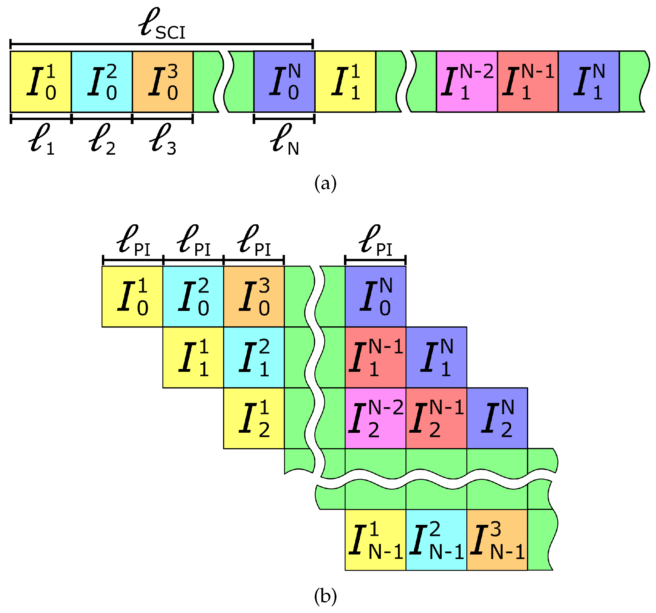
The set of tasks executed in one iteration is called Single-Cycle Iteration (SCI). Figure 1a shows the SCIs carried out in sequence, according to N instructions. The instructions are labeled as $I_i^n$, where $n\in \{1,2,\dots ,N\}$ is the instruction number and $i\in \{0,1,\dots ,\infty \}$ is the SCI number. Each instruction has its own latency, and the sum of the N latencies ${\sum }_{n=1}^N{\ell }_n$ from the same SCI corresponds to the SCI latency ${\ell }_{\mathrm{SCI}}$.

Figure 1. Execution techniques: (a) Nonpipeling. (b) Pipelining.

The pipelining technique is used to divide the instructions of an SCI in multiple steps. Thus, some dependencies are broken and instructions from different SCIs are overlapped during runtime. Figure 1b shows the pipeline technique. The instructions from a SCI are divided, hence, there are not dependencies inside the new-bundled iteration. This new iteration is called Pipelined Iteration (PI) with a new latency equal to $max\{{\ell }_1,{\ell }_2,\dots ,{\ell }_N\}$.

The implementation of the pipelining technique provides two main advantages: Parallelization and delivery time. The parallelization can be reached due to the broken dependencies that allows the execution of more than one instruction at the same time. As it is shown in Figure 1b, the instructions of the same column can be executed in parallel as long as hardware capability. The delivery time with nonpipeling technique of a SCI is ${\sum }_{n=1}^N{\ell }_n$ while the execution time with pipelining implementation is ${\ell }_{\mathrm{PI}}$, here, only the first SCI execution time takes $N·{\ell }_{\mathrm{PI}}$ to be delivered.

3.2. One-Step Ahead Prediction

The MPC approach assumes that with the system information been collected at each sampling instant $y\left(k\right)$, $\gamma \left(k\right)$, $x\left(k\right)$, $u(k-1)$, the control action $u\left(k\right)$ can be calculated instantaneously. However, the real-time implementation of this approach is mainly limited due to the optimization problem to be solved.

In the proposed algorithm, the controller parameters optimized from the previous sampling interval is used to calculate the current control action $u(k-1)$. By minimizing (10), $\Delta U\left(k\right)$, (9), is obtained subject to the constraints. Hence, the first vector corresponds to $\Delta u\left(k\right)$; thus, the current manipulation $u\left(k\right)$ can be computed as follows: $u\left(k\right)=\Delta u\left(k\right)+u(k-1)$. This breaks the bottleneck due to the dependencies carried out by the variables computed at the same iteration.

4. Study Cases

The present work and the MPC strategy in [10] are developed using the same computational platform. The study cases consider the following state-space models in continuous time, where $A_c\in {\mathbb{R}}^{n_x\times n_x}$ is the state matrix, $B_c\in {\mathbb{R}}^{n_x\times n_u}$ stands for the input matrix and $C_c\in {\mathbb{R}}^{n_x\times n_y}$ corresponds to the output matrix. Hence, the systems are discretized to be represented according to (1).

4.1. Study Case 1— Jet Transport Aircraft

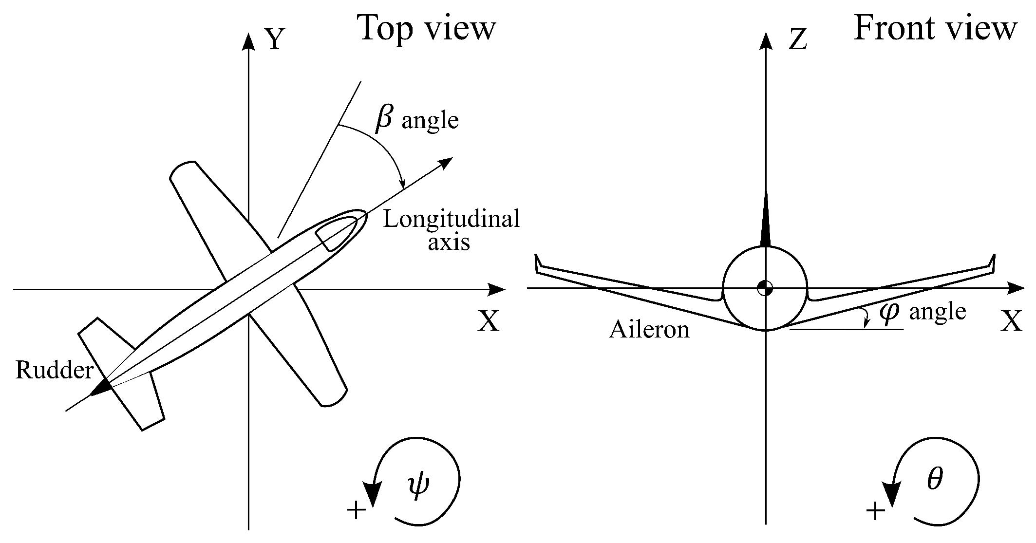
From [21,33,34], a Jet Transport Aircraft Boeing 747 is obtained. In high-lift configuration, it addresses complex geometries and physical phenomena that make the controller design a difficult process. Figure 2 illustrates the Jet Transport Aircraft with its components and variables involved such as the angles $\beta$ and $\varphi$ and the angular velocities $\psi$ and $\theta$.

Figure 2. Jet transport aircraft.

Although the physical model of the Boeing 747 is lengthy, in (18), the simplified state-space model during cruise flight at MATCH = 0.8 and H = 40,000 ft is presented in continuous time:

$$\begin{array}{ccc}\hfill \dot{x}\left(t\right)& =& A_{c}x\left(t\right)+B_{c}u\left(t\right),\hfill \\ \hfill y\left(t\right)& =& C_{c}x\left(t\right),\hfill \end{array}$$

(18)

where

$$\begin{array}{ccc}\hfill A_c& =& \left[\begin{array}{cccc}-0.0558& -0.9968& 0.0802& 0.0415\\ 0.598& -0.115& -0.0318& 0\\ -3.05& 0.388& -0.465& 0\\ 0& 0.0805& 1& 0\end{array}\right]\hfill \\ \hfill B_c& =& \left[\begin{array}{cc}0.0729& 0\\ -4.75& 0.775\\ 0.153& 14.3\\ 0& 0\end{array}\right]\hfill \\ \hfill C_c& =& \left[\begin{array}{cccc}0& 1& 0& 0\\ 0& 0& 0& 1\end{array}\right]\hfill \end{array}$$

The model has four states, $x={\left[\begin{array}{cccc}\beta & \psi & \theta & \varphi \end{array}\right]}^T$, where $\beta$ is the sideslip angle, $\varphi$ stands for the bank angle, and meanwhile $\psi$ and $\theta$ represent the yaw and roll rate, respectively. Herein, all the angles are in rad and the angular velocities in rad/s. The system has two inputs $u={\left[\begin{array}{cc}{u}_1& u_2\end{array}\right]}^T$: the rudder and the aileron deflections, and two outputs $y={\left[\begin{array}{cc}{y}_1& y_2\end{array}\right]}^T$ the yaw rate $\psi$ and the bank angle $\varphi$. Then, using a sampling time $\tau =$ 0.2 s, the system is discretized and executed under the constraints described in Table 1.

Table 1. Jet transport aircraft constraints.

	Output		Input		Input Increment
	Yaw	Bank	Rudder	Aileron	Incremental Rudder	Incremental Aileron
	Rate	Angle	Deflection	Deflection	Deflection	Deflection
Maximum	1	1	4	4	1	1
Minimum	−1	−1	−4	−4	−1	−1

4.2. Study Case 2—Tape Transport System

The tape drive system consists of two reels to supply and file data. Here, the data transfer rate is proportional to the tape transport speed.Thus, the tape drive mechanism must be able to rapidly transport a fragile tape with an accurate tension regulation. Figure 3 shows the schematic of a tape transport system where its components and variables involved are the tape stiffness and the damping denoted by K and D, the reel radii and the inertia represented as r and J, the motor torque constant $K_t$, and the viscous friction coefficient denoted by $\beta$.

Figure 3. Tape transport system.

Assuming there is no force loss across the head, the tape tension $T=T_1=T_2$ [35]. Although the physical model of the process contains nonlinearities, in (19), a simplified state-space model is presented in continuous time [21,35,36,37]:

$$\begin{array}{ccc}\hfill \dot{x}\left(t\right)& =& A_{c}x\left(t\right)+B_{c}u\left(t\right),\hfill \\ \hfill y\left(t\right)& =& C_{c}x\left(t\right),\hfill \end{array}$$

(19)

where

$$\begin{array}{ccc}\hfill A_c& =& \left[\begin{array}{ccc}-D\left(\frac{r_1^2}{J_1}+\frac{r_2^2}{J_2}\right)& D\frac{\beta r_1}{J_1}-\frac{K}{r_1}& \frac{K}{r_2}-D\frac{\beta r_2}{J_2}\\ \frac{r_1}{J_1}& -\frac{\beta }{J_1}& 0\\ -\frac{r_2}{J_2}& 0& -\frac{\beta }{J_2}\end{array}\right]\hfill \\ \hfill B_c& =& \left[\begin{array}{cc}-D{K}_t\frac{r_1}{J_1}& D{K}_t\frac{r_2}{J_2}\\ \frac{K_t}{J_1}& 0\\ 0& \frac{K_t}{J_2}\end{array}\right]\hfill \\ \hfill C_c& =& \left[\begin{array}{ccc}0& \frac{r_1}{2}& \frac{r_2}{2}\\ 1& 0& 0\end{array}\right]\hfill \end{array}$$

The model has three states, $x={\left[\begin{array}{ccc}T& {\omega }_1& {\omega }_2\end{array}\right]}^T$, where T is the tension tape in N; meanwhile, ${\omega }_1$ and ${\omega }_2$ represent the supply and take-up reel in rad/s, respectively. Moreover, the system has two inputs $u={\left[\begin{array}{cc}{u}_1& u_2\end{array}\right]}^T$ that represent the voltages applied to the reel motors in volts, and two outputs $y={\left[\begin{array}{cc}{y}_1& y_2\end{array}\right]}^T$ which stand for the tape speed $v_{rw}$ at the read-write head in m/s and the tape tension T, respectively. The control strategy described in the present work is simulated using parameters from the tested tape system described in [35,38,39], whose parameters are summarized in Table 2.

Table 2. Tape transport system parameters.

Symbol	Parameter	Value
K	Tape stiffness	$2\times {10}^3$ N/m
D	Damping	2 N s/m${}^2$
$r_1$	Radius of supply reel	$21.2\times {10}^{-3}$ m
$r_2$	Radius of take-up reel	$9.75\times {10}^{-3}$ m
$J_1$	Moment of inertia of the supply reel	$14.2\times {10}^{-6}$ kg m${}^2$
$J_2$	Moment of inertia of take-up reel	$10.35\times {10}^{-6}$ kg m${}^2$
$K_t$	Motor torque constant	$24.8\times {10}^{-3}$ N m/V
$\beta$	Viscous friction coefficient	$1.03\times {10}^{-4}$ N m s/rad

Considering that the motors are nominally identical, for both motors, it is used as the same motor torque constant $K_t$ and viscous friction coefficient $\beta$ [38,39]. Thus, using a sampling time $\tau =0.1$ s, the system (19) is discretized and executed under the constraints expressed in Table 3.

Table 3. Tape transport system constraints.

	Output		Input		Input Increment
	Tape	Tape	Motor	Motor	Incremental Motor	Incremental Motor
	Speed	Tension	Voltage	Voltage	Voltage	Voltage
Maximum	3	0.8	2	0.4	1	1
Minimum	0	0	−1	−0.1	−1	−1

5. Proposed Software-Based Implementation

5.1. Profile Analysis

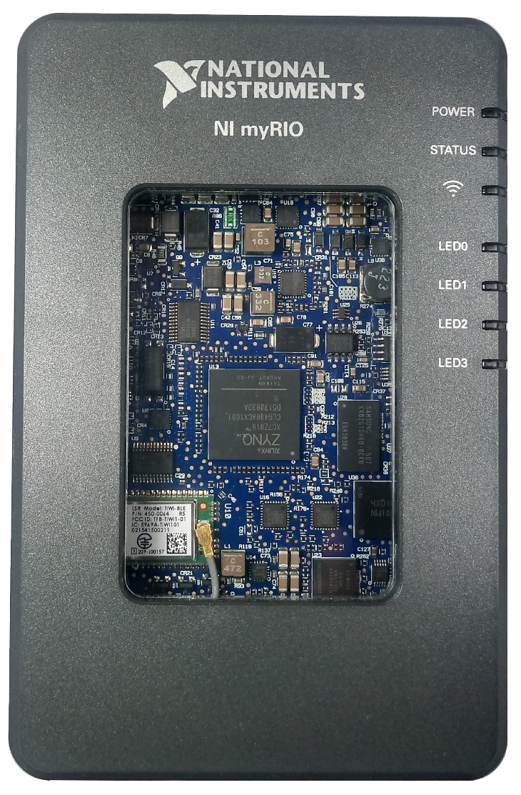
The profiling analysis is performed on a NI myRIO 1900, illustrated in Figure 4, from National Instruments [40]. The NI myRIO is a portable reconfigurable I/O (RIO) device that can be used to design control, robotics, and mechatronics systems. The NI myRIO contains a Xilinx Z-7010 System-on-Chip (SoC), working at a frequency of 650 MHz.

Figure 4. NI myRIO 1900.

The Xilinx Z-7010 SoC has an architecture divided in two parts: a processing system (PS) and a programmable logic. The PS includes 256 KB on-chip memory, 8 Direct Memory Access (DMA) channels, external memory interfaces, and multiple I/O peripherals. The main component of the PS is the application processor unit (APU) which contains a dual-core ARM Cortex-A9 for running the application software. The ARM cores use the ARMv7 architecture.

Although the NI myRIO can be considered a high-speed processing device compared to the microprocessor in [22,26,27]. In contrast with those with acceptable implementation for high speed applications [23,24,25], it can still be considered as a low resources processor.

The process flow diagram of the baseline MPC algorithm is shown in Figure 5. As it can be seen, it is composed of two types of functions: offline and online. The offline functions are one-time executed, while the online functions are executed each sampling time. Table 4 and Table 5 shows the description of each function and the latency according to the study case 1.

Figure 5. Process flow diagram of the MPC algorithm.

Table 4. Offline functions.

Function	Description	Latency
MPC Offline	It contains the matrices of the State-Space Model and the VFM, the sampling time, the prediction and control horizon, the constraints and the matrices $E,F_1,F_2,M,I_1,\mathrm{\Psi }$ and $\mathrm{\Phi }$.	$4183.580\mathsf{\mu }\mathrm{s}$
Init	It initializes the control vector $u_k$	$\mathrm{86,718.800}\mathsf{\mu }\mathrm{s}$

Table 5. Online functions.

Function	Description	Latency
RDSen	It reads the controlled variable $y\left(k\right)$.	22.532 $\mathsf{\mu }\mathrm{s}$
SPGen	It generates the setpoint $r_s\left(k\right)$.	$14.509\mathsf{\mu }\mathrm{s}$
Obs	It measures the current x(k) vector.	$52.378\mathsf{\mu }\mathrm{s}$
FCalc	It computes the vector $F\left(k\right)=F_{1}x\left(k\right)+F_2{R}_s$.	$80.698\mathsf{\mu }\mathrm{s}$
$\gamma$Calc	It computes the vector $\gamma \left(k\right)$.	$63.821\mathsf{\mu }\mathrm{s}$
Optim	It computes the optimal manipulated variable $u\left(k\right)$.	$1290.780\mathsf{\mu }\mathrm{s}$
WRAct	It applies the manipulated variable $u\left(k\right)$.	$39.202\mathsf{\mu }\mathrm{s}$
Graph	It plots the variables $y\left(k\right)$, $u\left(k\right)$, $\Delta u$ and the constraints.	$37.468\mathsf{\mu }\mathrm{s}$

5.2. Software-Based Implementation Development

To improve the computing performance, a proposed software-based implementation is developed based on the profiling analysis of the online functions (Table 5) and the computer architecture concepts described in Section 3. Thus, the following improvements are implemented: efficient calculation of the optimization algorithm, implementing pipelining. This work apply three different methods to achieve a better performance. In Table 5, it can be seen that the Optim function has the highest latency. Thus, the present research work first proposes to speed it up by modifying the Hildreth’s algorithm. Then, the concept of pipelining is applied, and the optim function is parallelized with the rest of the functions. However, a problem shows up through the implementation. Therefore, the prediction idea is carried out to solve this problem.

5.2.1. Optimization Algorithm

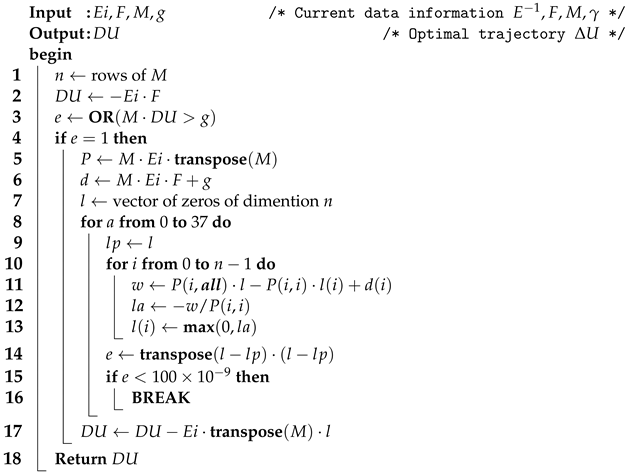
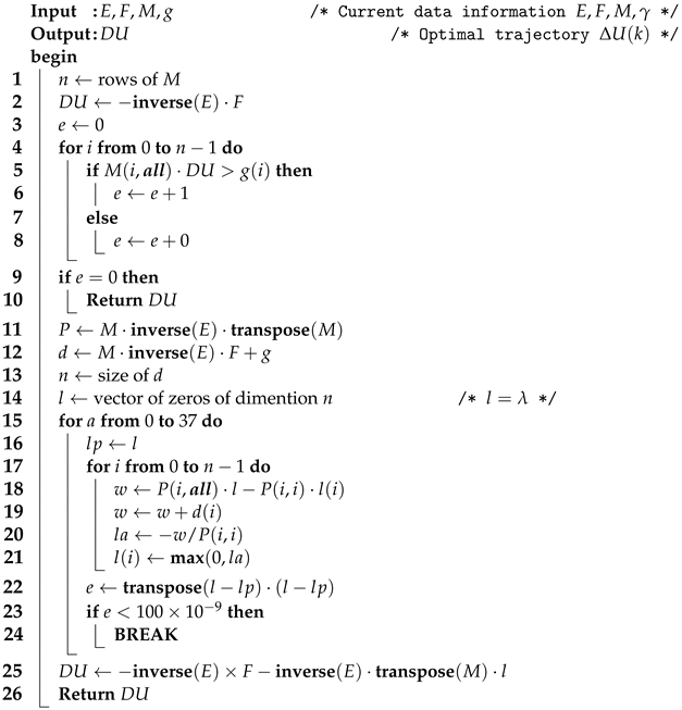
The baseline algorithm uses the Hildreth’s Quadratic Programming Solver (qpSolver), shown in Algorithm 1, to minimized the objective function. Nevertheless, there are two weaknesses that increase the execution time of the Optim function: the operations recurrence and the operation of array elements. The operational recurrence was solved by reusing the previously calculated data. The calculation of the inverse of the E matrix should be highlighted, as it is mentioned in [41]. The E matrix is not modified during the execution, following this, the inverse operation can be calculated once. For this reason, the new algorithm requires the $E^{-1}$ as an input, and the inversion operation is calculated in the MPC Offline function. The operation of arrays elements was boosted using optimized functions that works directly with arrays instead of the elements. The modified algorithm can be seen in Algorithm 2. A new profile analysis was performed, with these modifications, thus, the latency of the Optim function is reduced from $1290.78$ $\mathsf{\mu }\mathrm{s}$ to $226.75$ $\mathsf{\mu }\mathrm{s}$ for the study case 1 and from 3491 $\mathsf{\mu }\mathrm{s}$ to 394 $\mathsf{\mu }\mathrm{s}$ for the study case 2.

Algorithm 1: Hildreth’s QP Solver (Original)

Algorithm 2: Hildreth’s QP Solver (Improved)

5.2.2. Pipelining

The Online functions from every SCI, shown in Table 5, can be arranged in 3 bundles. Bundle 1 (Latency: $233.938$ $\mathsf{\mu }\mathrm{s}$) packs functions RDSen, SPGen, Obs, Fcalc, and $\gamma$Calc. Bundle 2 (Latency: $226.75$ $\mathsf{\mu }\mathrm{s}$) include the modified Optim function. Bundle 3 (Latency: $76.670$ $\mathsf{\mu }\mathrm{s}$) packs functions WRAct and Graph. The concept of pipelining, Section 3.1 can be extrapolated to work with bundles instead of instructions for both study cases. Figure 6 uses the notation $B_k^n$ to indicate the bundle n of the SCI k. As show in Figure 6a, the execution is performed running a bundle per step. In Figure 6b, Bundle 1 and 3 are executed in the same step, in order to balance the time execution between step 1 ($310.608$ $\mathsf{\mu }\mathrm{s}$) and 2 ($226.750$ $\mathsf{\mu }\mathrm{s}$). Currently, the bundles $B_k^1$, $B_{k-1}^2$, $B_{k-1}^3$ are run within the same PI.

Figure 6. Optimization methodology: (a) Executing a bundle per step. (b) Executing Bundle 1 and Bundle 3 in the same step. (c) Executing Bundle 1 and Bundle 3 in the same step, and implementing Optim+Function.

5.2.3. Synchronization Error Troubleshooting

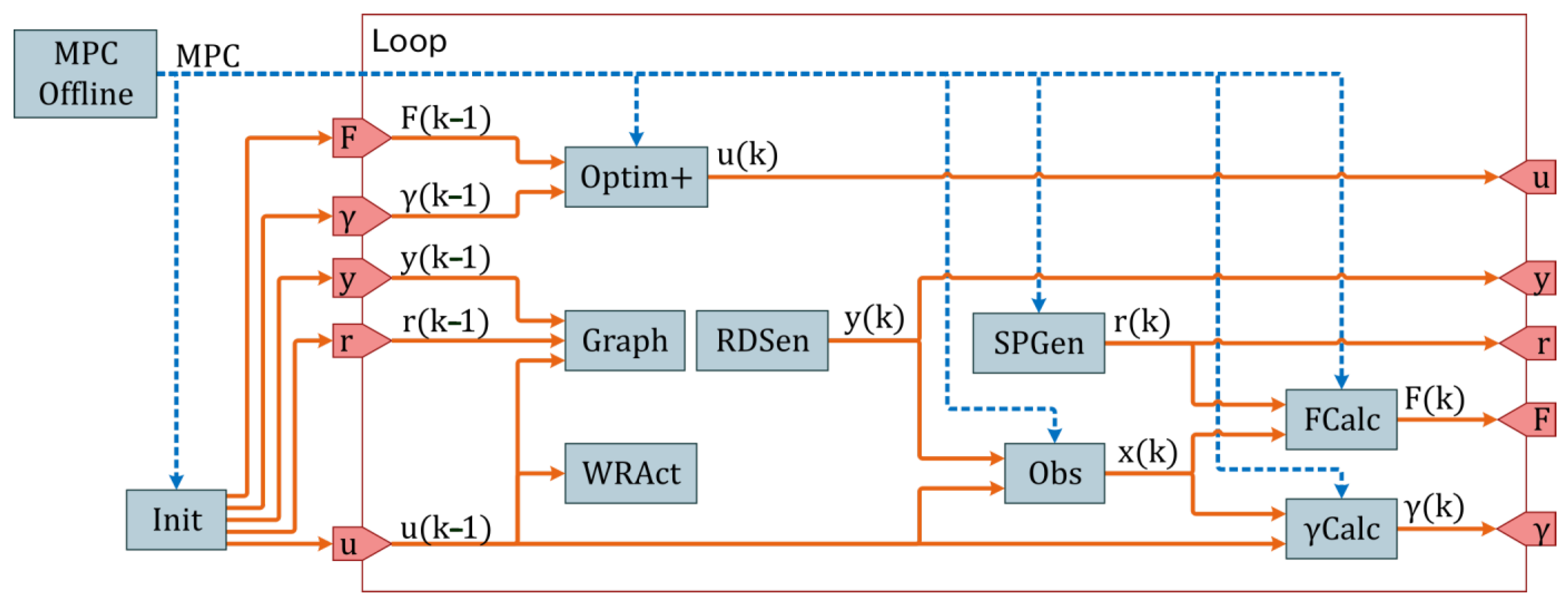
Using the Figure 5 as reference, a synchronization error can be noticed in node A of the Figure 6a,b. In Figure 6b, $B_k^1$ (Function Obs and $\gamma$Calc) and $B_{k-1}^3$ (Function WRAct and Graph) needs $u(k-1)$ as input, but they are receiving $u(k-2)$. The bundle $B_k^2$ represent the Optim function that can be seen in Algorithm 3. The Optim function calculates $u\left(k\right)$ based on the iteration data $F\left(k\right),\gamma \left(k\right)$. A modification of the algorithm Optim can take place. The Algorithm 4, shows a new Optim function called Optim+. The Optim+ function takes advantage of the QP Solver definition to compute the optimal $u\left(k\right)$ based on the previous iteration data $F(k-1)$ and $\gamma (k-1)$. In Figure 6c, the $B_k^{2+}$ (Optim+ function) is implemented to solve the synchronization error.

Algorithm 3: Optim function

Algorithm 4: Optim+ function

Finally, the implementation proposed to the MPC algorithm (Figure 5) can be observed in Figure 7.

Figure 7. Proposed process flow diagram of the MPC algorithm.

6. Results

The present work and the baseline algorithm VFM in [10] are developed using the same computational platform for the study cases described in Section 4. These implementations are analyzed considering: the speedup and the processor performance.

The speedup factor is described using (20).

$$Speedup=\frac{{\ell }_{\mathrm{Old}}}{{\ell }_{\mathrm{New}}}$$

(20)

where ${\ell }_{\mathrm{Old}}$ is the latency of the reference algorithm, and ${\ell }_{\mathrm{New}}$ is the latency of the proposed algorithm. On the other hand, the processor performance is evaluated considering the processor usage.

6.1. Study Case 1—Results

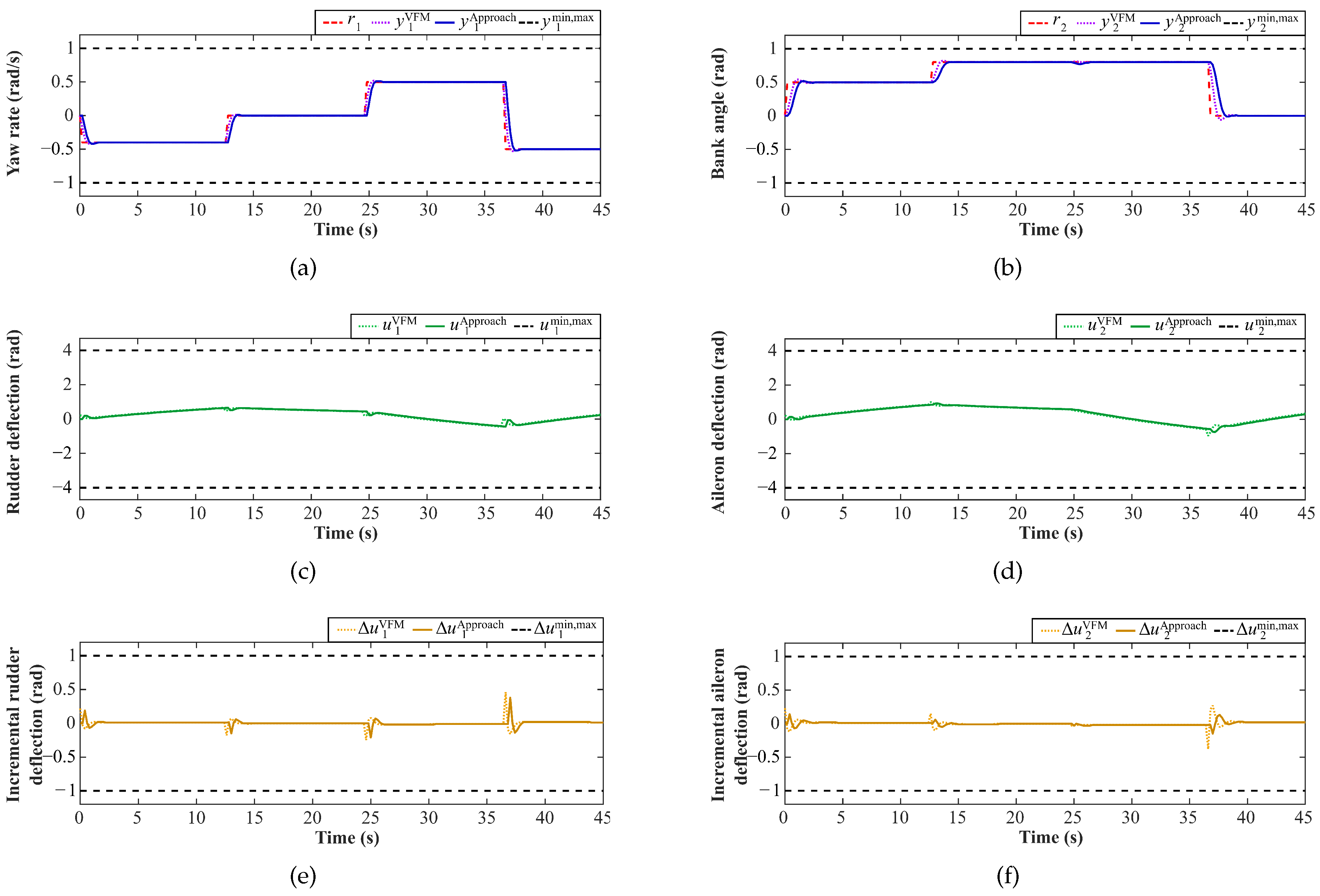
Considering a prediction horizon $N_p=20$, $N_c=15$ and a $R_u=I_{30\times 30}$, the simulation results are shown in Figure 8, the controlled variable, the manipulated variables, and the incremental variable are plotted for both: the present work and the baseline algorithm.

Figure 8. Results for the jet transport aircraft under VFM and Approach: (a) Yaw rate. (b) Bank angle. (c) Rudder deflection. (d) Aileron deflection. (e) Incremental rudder deflection. (f) Incremental aileron deflection.

Both implementations execute 1000 iterations, and a profile analysis is executed. The results from the profile analysis is shown in Table 6.

Table 6. Execution time comparison.

	VFM	Approach
Performance	$372.603$ Hz	$1713.920$ Hz
Average	2684 $\mathsf{\mu }\mathrm{s}$	583 $\mathsf{\mu }\mathrm{s}$
Variance ($s^2$)	$802.83\times {10}^{-9}$	$8.19\times {10}^{-9}$
Maximum	7634 $\mathsf{\mu }$s	1517 $\mathsf{\mu }$s

First, an enhancement is obtained by the implementation of the improvements to the Hildreth’s Algorithm. This reduces its latency from $1290.78$ $\mathsf{\mu }\mathrm{s}$ to $226.75$ $\mathsf{\mu }\mathrm{s}$. Reducing the execution time by 1064 $\mathsf{\mu }\mathrm{s}$. Then, the strategy of pipelining is implemented making an additional reduction of 1037 $\mathsf{\mu }\mathrm{s}$. Thus, the total execution time is reduced 2101 $\mathsf{\mu }\mathrm{s}$. Additionally, the speedup factor is calculated according to the execution times average presented in Table 6. Here, the speedup factor is $4.6\times$, ($50.64\%$ by the Hildreth’s modification and $49.35\%$ by the pipeline implementation).

Furthermore, considering that both implementations are run in multicore execution, the processor utilization is evaluated, Table 7.

Table 7. Processor usage comparison.

	VFM	Approach
CPU 0	$79.22\%$	$43.29\%$
CPU 1	$56.07\%$	$40.48\%$

As it can be seen, with the present research work, the processor usage was released $35.93\%$ for CPU 0 (from $79.22\%$ to $43.29\%$) and $15.59\%$ for CPU 1 (from $56.07\%$ to $40.48\%$).

6.2. Study Case 2—Results

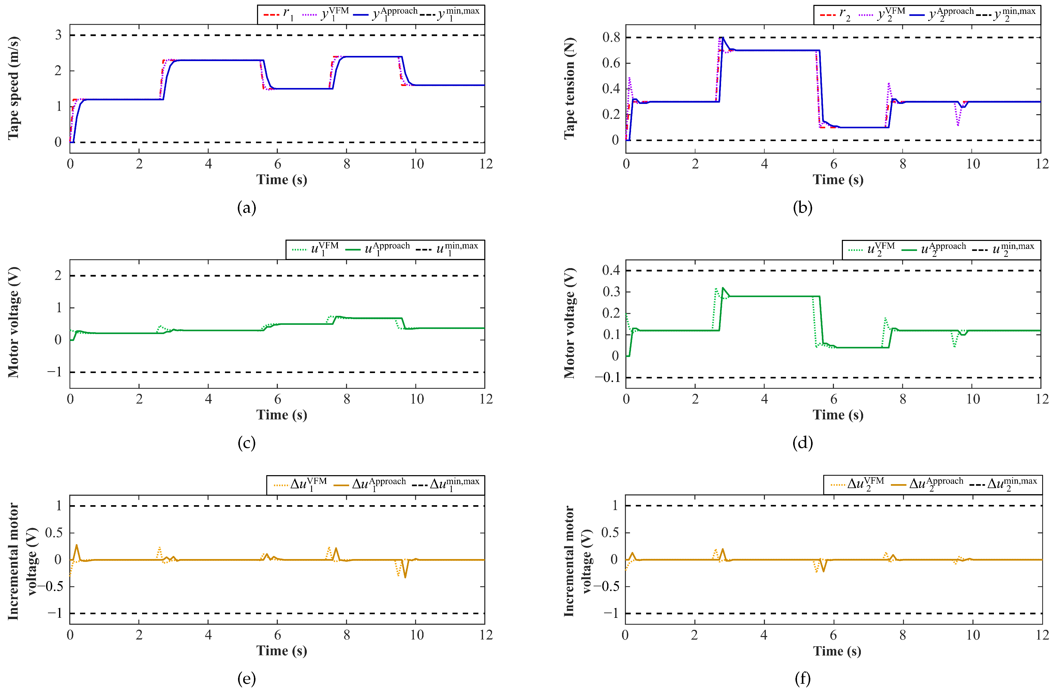
Considering a prediction horizon $N_p=20$, $N_c=15$ and a $R_u=I_{30\times 30}$, the simulation results are shown in Figure 9, the controlled variable, the manipulated variables, and the incremental variable are plotted for both: the present work and the baseline algorithm.

Figure 9. Results for the tape transport system under VFM and Approach: (a) Tape speed. (b) Tape tension. (c) Motor voltage supply reel. (d) Motor voltage take-up reel. (e) Incremental motor voltage supply reel. (f) Incremental motor voltage take-up reel.

Both implementations execute 1000 iterations, and a profile analysis is executed. The results from the profile analysis is shown in Table 8.

Table 8. Execution time comparison.

	VFM	Approach
Performance	$170.736$ Hz	$541.7118$ Hz
Average	5857 $\mathsf{\mu }\mathrm{s}$	1846 $\mathsf{\mu }\mathrm{s}$
Variance ($s^2$)	$5.46\times {10}^{-20}$	$2.08\times {10}^{-19}$
Maximum	$\mathrm{39,660}$$\mathsf{\mu }$s	$\mathrm{27,093}$$\mathsf{\mu }$s

According to the implementation of the modified Hildreth’s Algorithm, latency is considerably reduced from 3491 $\mathsf{\mu }\mathrm{s}$ to 394 $\mathsf{\mu }\mathrm{s}$. Thus, the execution time is reduced 3097 $\mathsf{\mu }\mathrm{s}$. Additionally, when the strategy of pipelining is implemented making an additional reduction of $914.1$ $\mathsf{\mu }\mathrm{s}$. Thus, the total execution time is reduced 4011 $\mathsf{\mu }\mathrm{s}$. Additionally, the speedup factor is calculated according to the execution times average presented in Table 8. Here, the speedup factor is $3.17\times$, ($72.21\%$ by the Hildreth’s modification and $22.79\%$ by the pipeline implementation).

Furthermore, considering that both implementations are run in multicore execution, the processor utilization is evaluated, Table 9.

Table 9. Processor usage comparison.

	VFM	Approach
CPU 0	$82.50$%	$53.49$%
CPU 1	$70.40$%	$56.84$%

As it can be seen, with the present research work, the processor usage was released $29.01\%$ for CPU 0 (from $82.50\%$ to $53.49\%$) and $13.56\%$ for CPU 1 (from $70.40\%$ to $56.84\%$).

7. Conclusions

This paper proposes a new software-based implementation for a constrained Multi-Input-Multi-Output predictive control algorithm embedded in the NI myRIO 1900 using NI LabVIEW Real-Time Module. Based on the computer architecture concepts, a software-based implementation is proposed. Thus, as an evaluation case, the proposed implementation is used to control a jet transport aircraft during cruise flight.

Experimental results shows that the new software-based implementation has a good performance regardless the computational modification effected. Additionally, compared with the baseline algorithm implementations, there is a significant improvement on the execution time without affecting the tracking performance for both study cases. The proposed software-based implementation reaches a speedup factor up to $4.6\times$ for the jet transport aircraft and $3.17\times$ for the tape transport system with respect to the baseline implementation. In addition, the processor usage was released for both study cases, $35.93\%$ and $29.01\%$ in CPU 0 and $15.59\%$ and $13.56\%$ in CPU 1, respectively. Thus, the obtained results do benefit the implementation of MIMO MPC techniques by reducing the execution time and the computational load.

References

- Jeng, J.C.; Chang, Y.J.; Lee, M.W. Novel design of dynamic matrix control with enhanced decoupling control performance. In Computer Aided Chemical Engineering; Elsevier B.V.: Amsterdam, The Netherlands, 2018; Volume 44, pp. 541–546. [Google Scholar] [CrossRef]
- Abro, G.E.M.; Zulkifli, S.A.B.; Ali, Z.A.; Asirvadam, V.S.; Chowdhry, B.S. Fuzzy Based Backstepping Control Design for Stabilizing an Underactuated Quadrotor Craft under Unmodelled Dynamic Factors. Electronics 2022, 11, 999. [Google Scholar] [CrossRef]
- Musa, A.; Pipicelli, M.; Spano, M.; Tufano, F.; De Nola, F.; Di Blasio, G.; Gimelli, A.; Misul, D.A.; Toscano, G. A Review of Model Predictive Controls Applied to Advanced Driver-Assistance Systems. Energies 2021, 14, 7974. [Google Scholar] [CrossRef]
- Liu, F.; Li, H.; Liu, L.; Zou, R.; Liu, K. A control method for IPMSM based on active disturbance rejection control and model predictive control. Mathematics 2021, 9, 760. [Google Scholar] [CrossRef]
- Bécsi, T. Quasi-Linear Parameter Varying Modeling and Control of an Electromechanical Clutch Actuator. Mathematics 2022, 10, 1473. [Google Scholar] [CrossRef]
- awryńczuk, M.; Marusak, P.M.; Chaber, P.; Seredyński, D. Initialisation of Optimisation Solvers for Nonlinear Model Predictive Control: Classical vs. Hybrid Methods. Energies 2022, 15, 2483. [Google Scholar] [CrossRef]
- Zavitsanou, S.; Chakrabarty, A.; Dassau, E.; Doyle, F.J. Embedded control in wearable medical devices: Application to the artificial pancreas. Processes 2016, 4, 35. [Google Scholar] [CrossRef]
- Baca, T.; Loianno, G.; Saska, M. Embedded Model Predictive Control of Unmanned Micro Aerial Vehicles. In Proceedings of the 2016 21st International Conference on Methods and Models in Automation and Robotics (MMAR), Miedzyzdroje, Poland, 29 August–1 September 2016; pp. 992–997. [Google Scholar] [CrossRef]
- Ibañez, C.; Ocampo-Martinez, C.; Gonzalez, B. Embedded optimization-based controllers for industrial processes. In Proceedings of the 2017 IEEE 3rd Colombian Conference on Automatic Control (CCAC), Cartagena, Colombia, 18–20 October 2017; pp. 1–6. [Google Scholar] [CrossRef]
- Wang, L. Model Predictive Control System Design and Implementation Using MATLAB, 1st ed.; Springer: Perth, Australia, 2009. [Google Scholar] [CrossRef]
- Vazquez, S.; Rodriguez, J.; Rivera, M.; Franquelo, L.G.; Norambuena, M. Model predictive control for power converters and drives: Advances and trends. IEEE Trans. Ind. Electron. 2016, 64, 935–947. [Google Scholar] [CrossRef]
- Karamanakos, P.; Geyer, T. Guidelines for the design of finite control set model predictive controllers. IEEE Trans. Power Electron. 2019, 35, 7434–7450. [Google Scholar] [CrossRef]
- Hu, J.; Ding, B. One-step ahead robust MPC for LPV model with bounded disturbance. Eur. J. Control 2020, 52, 59–66. [Google Scholar] [CrossRef]
- Zafra, E.; Vazquez, S.; Guzman Miranda, H.; Sanchez, J.A.; Marquez, A.; Leon, J.I.; Franquelo, L.G. Efficient FPSoc prototyping of FCS-MPC for three-phase voltage source inverters. Energies 2020, 13, 1074. [Google Scholar] [CrossRef]
- Luo, Q.; Nguyen, A.T.; Fleming, J.; Zhang, H. Unknown input observer based approach for distributed tube-based model predictive control of heterogeneous vehicle platoons. IEEE Trans. Veh. Technol. 2021, 70, 2930–2944. [Google Scholar] [CrossRef]
- Ju, Z.; Zhang, H.; Tan, Y. Distributed stochastic model predictive control for heterogeneous vehicle platoons subject to modeling uncertainties. IEEE Intell. Transp. Syst. Mag. 2021, 14, 25–40. [Google Scholar] [CrossRef]
- Pang, H.; Liu, M.; Hu, C.; Liu, N. Practical Nonlinear Model Predictive Controller Design for Trajectory Tracking of Unmanned Vehicles. Electronics 2022, 11, 1110. [Google Scholar] [CrossRef]
- Lee, T.; Kang, Y. Performance Analysis of Deep Neural Network Controller for Autonomous Driving Learning from a Nonlinear Model Predictive Control Method. Electronics 2021, 10, 767. [Google Scholar] [CrossRef]
- Richter, S.; Jones, C.N.; Morari, M. Real-time input-constrained MPC using fast gradient methods. In Proceedings of the IEEE Conference on Decision and Control, Shanghai, China, 15–18 December 2009. [Google Scholar] [CrossRef]
- He, M.; Ling, K.V. Model Predictive Control On A Chip. In Proceedings of the 2005 International Conference on Control and Automation, Budapest, Hungary, 26–29 June 2005; pp. 528–532. [Google Scholar] [CrossRef]
- Sotelo, D.; Favela-Contreras, A.; Kalashnikov, V.V.; Sotelo, C. Model Predictive Control with a Relaxed Cost Function for Constrained Linear Systems. Math. Probl. Eng. 2020, 2020, 7485865. [Google Scholar] [CrossRef]
- Bang, H.; Lee, Y.S. Embedded Model Predictive Control for Enhancing Tracking Performance of a Ball-and-Plate System. IEEE Access 2019, 7, 39652–39659. [Google Scholar] [CrossRef]
- Hýl, R.; Wagnerová, R. Design and Realization of Embedded Model Predictive Controller with Software Support. In Proceedings of the 2016 17th International Carpathian Control Conference (ICCC), Tatranska Lomnica, Slovakia, 29 May 2016–1 June 2016; pp. 259–264. [Google Scholar] [CrossRef]
- Yu, L.; Goldsmith, A.; Di Cairano, S. Efficient convex optimization on GPUs for embedded model predictive control. In Proceedings of the General Purpose GPUs, GPGPU-10 2017, Austin, TX, USA, 4–8 February 2017; pp. 12–21. [Google Scholar] [CrossRef]
- Cimini, G.; Bernardini, D.; Levijoki, S.; Bemporad, A. Embedded Model Predictive Control With Certified Real-Time Optimization for Synchronous Motors. IEEE Trans. Control Syst. Technol. 2020. [Google Scholar] [CrossRef]
- Boshkovski, G.; Stojanovski, G.; Stankovski, M. Development of embedded model predictive controller. In Proceedings of the 2017 13th IEEE International Conference on Control & Automation (ICCA), Ohrid, Macedonia, 3–6 July 2017; pp. 76–81. [Google Scholar] [CrossRef]
- Nermin, H.; Prljaca, N. An Implementation and Evaluation of Fast Embedded Model Predictive Control. In Proceedings of the 2020 19th International Symposium INFOTEH-JAHORINA (INFOTEH), East Sarajevo, Bosnia and Herzegovina, 18–20 March 2020. [Google Scholar]
- Wang, W.C.; Liu, T.H.; Syaifudin, Y. Model Predictive Controller for a Micro-PMSM-Based Five-Finger Control System. IEEE Trans. Ind. Electron. 2016, 63, 3666–3676. [Google Scholar] [CrossRef]
- Guzman, R.; De Vicuna, L.G.; Camacho, A.; Miret, J.; Rey, J.M. Receding-Horizon Model-Predictive Control for a Three-Phase VSI with an LCL Filter. IEEE Trans. Ind. Electron. 2019, 66, 6671–6680. [Google Scholar] [CrossRef]
- Pannocchia, G.; Gabiccini, M.; Artoni, A. Offset-free MPC explained: Novelties, subtleties, and applications. IFAC-PapersOnLine 2015, 48, 342–351. [Google Scholar] [CrossRef]
- Sotelo, C.; Favela-Contreras, A.; Beltrán-Carbajal, F.; Dieck-Assad, G.; Rodríguez-Cañedo, P.; Sotelo, D. A Novel Discrete-time Nonlinear Model Predictive Control Based on State Space Model. Int. J. Control. Autom. Syst. 2018, 16, 2688–2696. [Google Scholar] [CrossRef]
- Alamir, M. A Pragmatic Story of Model Predictive Control: Self-Contained Algorithms and Case-Studies; CreateSpace Independent Publishing Platform: Scotts Valley, CA, USA, 2013. [Google Scholar]
- Singh, S.; Murthy, T.V.R. Simulation of sensor failure accommodation in flight control system of transport aircraft a modular approach. World J. Model. Simul. 2015, 11, 55–68. [Google Scholar]
- Singh, S.; Rama Murthy, T. Design of an optimal yaw damper for 747 jet aircraft model. In Emerging Research in Electronics, Computer Science and Technology; Springer: Berlin/Heidelberg, Germany, 2014; pp. 801–810. [Google Scholar]
- Mathur, P.D.; Messner, W.C. Controller development for a prototype high-speed low-tension tape transport. IEEE Trans. Control Syst. Technol. 1998, 6, 534–542. [Google Scholar] [CrossRef]
- Lu, Y.; Messner, W.C. Robust servo design for tape transport. In Proceedings of the 2001 IEEE International Conference on Control Applications (CCA’01) (Cat. No. 01CH37204), Mexico City, Mexico, 7 September 2001; pp. 1014–1019. [Google Scholar]
- Tenne, D.; Singh, T. Robust feed-forward/feedback design for tape transport. In Proceedings of the AIAA Guidance, Navigation, and Control Conference and Exhibit, Providence, RI, USA, 16–19 August 2004; p. 5119. [Google Scholar]
- Baumgart, M.D.; Pao, L.Y. Robust control of nonlinear tape transport systems with and without tension sensors. J. Dyn. Sys. Meas. Control. 2007, 129, 41–55. [Google Scholar] [CrossRef][Green Version]
- Baumgart, M.D.; Pao, L.Y. Robust control of tape transport systems with no tension sensor. In Proceedings of the 2004 43rd IEEE Conference on Decision and Control (CDC) (IEEE Cat. No. 04CH37601), Nassau, Bahamas, 14–17 December 2004; Volume 4, pp. 4342–4349. [Google Scholar]
- National Instruments. NI myRIO-1900. User Guide and Specifications; Technical report; National Instruments: Austin, TX, USA, 2013. [Google Scholar]
- Zhu, Q.; Onori, S.; Prucka, R. Pattern recognition technique based active set QP strategy applied to MPC for a driving cycle test. In Proceedings of the American Control Conference, Chicago, IL, USA, 1–3 July 2015; pp. 4935–4940. [Google Scholar] [CrossRef]
Publisher’s Note: MDPI stays neutral with regard to jurisdictional claims in published maps and institutional affiliations. |
© 2022 by the authors. Licensee MDPI, Basel, Switzerland. This article is an open access article distributed under the terms and conditions of the Creative Commons Attribution (CC BY) license (https://creativecommons.org/licenses/by/4.0/).