Total Controllability of Non-Autonomous Measure Evolution Systems with Non-Instantaneous Impulses and State-Dependent Delay

Abstract

This paper is concerned with the existence of mild solutions and total controllability for a class of non-autonomous measure evolution systems with non-instantaneous impulses and state-dependent delay. By using the theory of evolution family and Krasnoselskii’s fixed point theorem, the existence of mild solutions and total controllability for the considered systems is obtained. Finally, we give two applications to support the validity of the study.

1. Introduction

Many physical processes such as harvesting, natural disasters, shocks, etc., cause abrupt changes in their states at a certain moment. These sudden changes occur in a very short time and can be neglected compared to the whole duration of the process. They are estimated in the form of instantaneous impulses. In other words, if a finite number of disturbances occur at a fixed time during a continuous evolutionary process, it is modeled as impulsive differential equations (IDEs, for short). IDEs have widespread applications in several areas of science and engineering, for example, population dynamics, ecology, and network control systems with scheduling protocols (see [1,2,3,4,5] and references therein).

However, some dynamics of the evolution processes in pharmacotherapy cannot be modeled by instantaneous impulsive dynamical systems, for example, in the hemodynamical equilibrium of a person, the introduction of insulin into the bloodstream and the consequent absorption of the body are gradual processes and stay active for a finite time period. Therefore, Hernández and O’Regan [6] introduced a new class of impulses termed non-instantaneous impulses, which start at an arbitrary fixed point and stay active for a finite time interval. Later, Wang and Fěckan [7] extended this model to instantaneous and non-instantaneous IDEs, which are very important in the study of dynamics of evolutionary processes. Borah and Bora [8] studied the existence of mild solutions for semilinear evolution equations with non-instantaneous impulses by using fixed point theorem. For detailed results on the theory of non-instantaneous IDEs, see [7,8,9,10,11] and references therein.

On the other hand, a complex situation with infinitely many perturbation points in a finite time interval, known as the Zeno behavior [12], cannot be modeled by IDEs. Therefore, measure differential equations (MDEs) play a key role in dealing with this phenomenon. In the beginning, MDEs were established by Sharma et al. [13] and Pandit et al. [14]. Thenceforth, Satco [15] obtained the existence of regulated solutions of MDEs by applying fixed point theorem. Using Mönch fixed point theorem and measure of noncompactness, the existence results for the semilinear MDEs are investigated in [16].

As we know, controllability is an important concept in modern mathematical control theory, which has already gained considerable attention from many scholars [1,2,9,10,17,18]. For instance, Chalishajar and Kumar [9] studied the controllability of the second order semilinear differential equation with infinite delay and non-instantaneous impulses. A frequently used method for solving the controllability problem is to transform it into a fixed point problem for an appropriate operator in a function space. Existence and control problems for various types of measure differential systems have been studied by many authors in [19,20,21,22,23,24,25]. For example, Wan and Sun [24] investigated the approximate controllability for a class of abstract MDEs by applying $\rho$-set contractive fixed point theorem. In [23], Kumar and Abdal discussed the controllability for a class of MDEs with nonlocal conditions by using Mönch fixed point theorem.

More generally, Cao and Sun [20] proved the exact controllability for following the semilinear MDEs in Banach spaces

$$\left\{\begin{array}{c}dx\left(t\right)=A\left(t\right)x\left(t\right)+Bu\left(t\right)+f(t,x(t\left)\right)dg\left(t\right),t\in J=[0,b];\hfill \\ x\left(0\right)+p\left(x\right)=x_0.\hfill \end{array}\right.$$

By using semigroup theory and Mönch fixed point theorem, sufficient conditions for exact controllability of MDEs are established.

Wang et al. [11] investigated the exact controllability for the following fractional evolution system with non-instantaneous impulses

$$\left\{\begin{array}{c}{}^c{D}_{0,t}^{\alpha }v\left(t\right)\in F(t,v\left(t\right))+B\left(u\left(t\right)\right),t\in \left({\sigma }_i,{\tau }_{i+1}\right],i=0,1,\cdots ,m;\hfill \\ v\left({\tau }_i^{+}\right)=g_i\left({\tau }_i,v\left({\tau }_i^{-}\right)\right),i=1,\cdots ,m;\hfill \\ v\left(t\right)=g_i\left(t,v\left({\tau }_i^{-}\right)\right),t\in \left({\tau }_i,{\sigma }_i\right],i=1,\cdots ,m;\hfill \\ v\left(0\right)=v_0,\hfill \end{array}\right.$$

where $F:[0,b]\times X\to 2^X-\{Ø\}$ is a given multifunction, the fixed points ${\tau }_i$ and ${\sigma }_i$ satisfy $0={\sigma }_0<{\tau }_1<{\sigma }_1<{\tau }_2<...<{\tau }_m<{\sigma }_m<{\tau }_{m+1}=b,v\left({\tau }_i^{+}\right)$ and $v\left({\tau }_i^{-}\right)$ are the right and left limits of v at the point ${\tau }_i$ respectively, and $v_0\in X$ is a fixed point.

However, Wang et al. obtained exact controllability by only applying control in the last subinterval of time, not on each point of impulses. However, in many engineering applications, we also need to control the system within each impulse interval. Therefore, in this manuscript, the control is applied for each subinterval of time. So, we establish the so-called total controllability result of the evolution system. Moreover, there are various real-world phenomena, such as heat conduction in materials with decaying memory, inferred grinding models and neural networks, etc, that depend on the past states of the system and are described by the state-dependent delay evolution systems. Many authors have contributed to the solvability and controllability of such systems with state-dependent delay, see [2,9,10,17,18,23,26] and the references therein.

Motivated by the above-mentioned discussions, we consider the total controllability for the following non-autonomous measure evolution systems with non-instantaneous impulses and state-dependent delay

$$\left\{\begin{array}{c}{\displaystyle dx\left(t\right)=A\left(t\right)x\left(t\right)+[Bu\left(t\right)+f(t,x_{\rho (t,x_t)})]dg\left(t\right),t\in \bigcup _{k=0}^m(s_k,t_{k+1}];}\hfill \\ {\displaystyle x\left(t\right)=h_k(t,x_{\rho (t,x_t)}),t\in \bigcup _{k=1}^m(t_k,s_k];}\hfill \\ {\displaystyle x\left(t\right)+p\left(x\right(t\left)\right)=\phi \left(t\right),t\in (-\infty ,0],}\hfill \end{array}\right.$$

(1)

where $J=[0,a]$, $0<t_1<t_2<\cdots <t_m<t_{m+1}=a$, $s_0:=0$, and $s_k\in (t_k,t_{k+1})$ for each $k=1,2,\dots ,m$, $\phi \in {\mathcal{B}}_h$. ${\mathcal{B}}_h$ is a phase space, which will be specialized later in Section 2. $A\left(t\right)$ is a family of linear operators (not necessarily bounded) on X, where X is a Banach space. $f:J\times {\mathcal{B}}_h\to X$. The function $x_t:(-\infty ,0]\to X$ is an element of ${\mathcal{B}}_h$ and defined by $x_t\left(\theta \right)=x(t+\theta ),\theta \in (-\infty ,0]$. The function $\rho :J\times {\mathcal{B}}_h\to (-\infty ,a]$ is continuous. Moreover the function $p:X\to X$ is continuous. The control function $u(·)$ takes values in $HS{L}_g^2(J;U)$, where U is also a Banach space. $HL{S}_g^2(J;U)$ will be introduced in Section 2. B is a bounded linear operator from U into X. $h_k:(t_k,s_k]\times {\mathcal{B}}_h\to X$ is non-instantaneous impulsive function for all $k=1,2\dots m$. $g:J\to \mathbb{R}$ is a left continuous non-decreasing function on X. $dx$ and $dg$ denote the distributional derivatives of the solution and the function g, respectively.

The main contribution, importance, and novelty of this article are given below:

• The existence of a mild solution to the system (1), by applying an integral equation which is given in terms of semigroup, is established for the first time. Then, by using the theory of evolution family and Krasnoselskii’s fixed point theorem, we obtain some sufficient conditions to ensure the controllability of system (1).
• It should be pointed out that our system covers complex situations. If the function g is the sum of a step and an absolutely continuous function, the system exhibits both instantaneous and non-instantaneous impulses. Few papers have investigated such systems, so this is a new challenge for the scientific field to solve such problems separately.
• Moreover, we establish the total controllability result, where the control system (1) achieves the desired state at the last point and at each impulse point $t_{k+1}$.
• The significance to study the MDEs is that one can model Zeno trajectories because g as a function of bounded variation may exhibit infinitely many discontinuity points in a finite interval. Such systems arise in game theory, non-smooth mechanics, and other systems [12,27].
• As the authors of [10,22] said, the main difficulty to deal with the MDEs is that they are not as smooth or continuous as ordinary differential equations. This fact means that further study for MEDs is more difficult, mainly because they are only right continuous and bounded.
• The results of our derivation involve state-dependent delay and non-instantaneous impulses; therefore, they generalize the existing results of Cao [20] and Sun.
• Finally, we give two applications to support the validity of the study.

This paper is organized as follows. In Section 2, we first give some fundamental concepts and results, which will be used throughout this paper. Next, by using Krasnoselskii’s fixed point theorem, we obtain the controllability results for system (1) in Section 3. Finally, in Section 4, an illustrative example is worked out to support the main results.

2. Preliminaries

In this section, we list some necessary definitions and lemmas, which will be used throughout the present paper.

Definition 1

([15]). A function $f:[0,a]\to X$ is called regulated on $[0,a]$, if the limits

$$\underset{s\to t^{-}}{lim}f\left(s\right)=f\left(t^{-}\right)\mathrm{and}\underset{s\to t^{+}}{lim}f\left(s\right)=f\left(t^{+}\right)$$

exist and are finite for $t\in [0,a]$.

The space of regulated functions $f:[0,a]\to X$ is denoted by $G\left(\right[0,a];X)$. It is well known that the set of discontinuities of a regulated function is at most countable and that the space $G\left(\right[0,a];X)$ is a Banach space endowed with the norm ${\parallel f\parallel }_{\infty }={sup}_{t\in [0,a]}\{\parallel f\left(t\right)\parallel \}$.

Lemma 1

([19]). Consider the functions $f:[a,b]\to X$ and $g:[a,b]\to \mathbb{R}$ such that g is regulated and ${\int }_a^{b}fdg$ exists. Then for every $t_0\in [a,b]$, the function

$$h\left(t\right)={\int }_{t_0}^{t}f\left(s\right)dg\left(s\right),t\in [a,b]$$

is regulated.

Definition 2

([19]). A set $\mathbb{A}\in G\left(\right[a,b];X)$ is called equiregulated if, for every $\epsilon >0$ and every $t_0\in [a,b]$, there is $\delta >0$ such that

(i) if $x\in \mathbb{A},t\in [a,b]$, and $t_0-\delta <t<t_0$, then $\parallel x\left(t_0^{-}\right)-x\left(t\right)\parallel <\epsilon ,$

(ii) if $x\in \mathbb{A},t\in [a,b]$, and $t_0<t<t_0+\delta$, then $\parallel x\left(t\right)-x\left(t_0^{+}\right)\parallel <\epsilon .$

Lemma 2

([19]). Let X be a Banach space. Assume that $\mathbb{A}\subset G\left(\right[0,a];X)$ is equiregulated, and for every $t\in [0,a]$, the set $\left\{x\right(t):x\in \mathbb{A}\}$ is relatively compact in X. Then the set $\mathbb{A}$ is relatively compact in $G\left(\right[0,a];X)$.

Definition 3

([15]). A function $f:[a,b]\to X$ is called Henstock–Lebesgue–Stieltjes integrable on $[a,b)$ if there is a function denoted by ${\int }_0^{·}:[a,b]\to X$ such that for every $\epsilon >0$, there exists a gauge δ on $[a,b)$ with

$$\sum _{i=1}^n∥f\left({\xi }_i\right)\left(g\left(t_i\right)-g\left(t_{i-1}\right)\right)-\left({\int }_0^{t_i}f\left(s\right)dg\left(s\right)-{\int }_0^{t_{i-1}}f\left(s\right)dg\left(s\right)\right)∥<\epsilon$$

for every δ-fine partition $\left\{\left(\left[t_{i-1},t_i\right),{\xi }_i\right):i=1,2,\dots ,n\right\}$ of $[a,b)$.

Let $HL{S}_g^p(J;X)$ be a space of all p-ordered Henstock–Lebesgue–Stieltjes integral regulated functions from J to X with respect to g. The norm ${\parallel ·\parallel }_{HL{S}_g^p}$ is defined by

$${\parallel f\parallel }_{HL{S}_g^p}={\left({\int }_0^a{\parallel f\left(s\right)\parallel }^{p}dg\left(s\right)\right)}^{\frac{1}{p}}.$$

The control function $u\in HL{S}_g^2(J;U)$, where U is a separable reflexive Banach space. The space of all bounded linear operators from U to X is denoted by $\mathcal{L}(U;X)$ equipped with the norm ${\parallel ·\parallel }_{\mathcal{L}(U;X)}$. The notation $\mathcal{L}\left(X\right)$, represents the space of all bounded linear operators on X equipped with the norm ${\parallel ·\parallel }_{\mathcal{L}\left(X\right)}$.

Let $h:(-\infty ,0]\to (0,\infty )$ be a continuous function with $l={\int }_{-\infty }^{0}h\left(t\right)dt<\infty$. For any $\delta >0$, we define $\mathcal{B}=\{\phi :[-\delta ,0]\to X$ such that $\phi \left(t\right)$ is bounded and measurable} and equip the space with the norm

$${\parallel \phi \parallel }_{[-\delta ,0]}=\underset{s\in [-\delta ,0]}{sup}\left|\phi \left(s\right)\right|,\forall \phi \in \mathcal{B}.$$

Let us define ${\mathcal{B}}_h=\left\{\phi :(-\infty ,0]\to X\right.$ such that for any $c>0,{\left.\phi \right|}_{[-c,0]}\in \mathcal{B}$ with $\phi \left(0\right)=0$ and $\left.{\int }_{-\infty }^{0}h\left(s\right){\parallel \phi \parallel }_{[s,0]}ds<\infty \right\}$. If ${\mathcal{B}}_h$ is endowed with the norm

$${\parallel \phi \parallel }_{{\mathcal{B}}_h}={\int }_{-\infty }^{0}h\left(s\right){\parallel \phi \parallel }_{[s,0]}ds,\forall \phi \in {\mathcal{B}}_h,$$

then $\left({\mathcal{B}}_h,{\parallel ·\parallel }_{{\mathcal{B}}_h}\right)$ is a Banach space.

Next, we employ an axiomatic definition of the phase space ${\mathcal{B}}_h$ introduced by Hale and Kato [28] and follow the terminology used in [26]. The phase space ${\mathcal{B}}_h$ defined above also satisfies the following axioms:

(A1) If $x:(-\infty ,a]\to X$ such that $x_0\in {\mathcal{B}}_h$ and ${x|}_J\in G(J;X)$. Then the following conditions hold:

(i) $x_t\in {\mathcal{B}}_h$ for $t\in J$.

(ii) $\parallel x_t{\parallel }_{{\mathcal{B}}_h}\le \mathsf{\Lambda }\left(t\right)sup\{\parallel x\left(s\right)\parallel :0\le s\le t\}+\mathsf{{\rm Y}}\left(t\right)\parallel x_0{\parallel }_{{\mathcal{B}}_h}$ for $t\in J,$ where $\mathsf{\Lambda },\mathsf{{\rm Y}}$:$[0,\infty )\to [0,\infty )$ are independent of x, the function $\mathsf{\Lambda }(·)$ is strictly positive and continuous, $\mathsf{{\rm Y}}(·)$ is locally bounded.

(A2) The space ${\mathcal{B}}_h$ is complete.

For any $\phi \in {\mathcal{B}}_h$, the function ${\phi }_t$ for $t\le 0$, is defined as ${\phi }_t\left(\theta \right)=\phi (t+\theta ),\theta \in (-\infty ,0]$. Then for any function $x(·)$ satisfying the axiom (A1) with $x_0=\phi$, one can extend the mapping $t\mapsto x_t$ by setting $x_t={\phi }_t,t\le 0$, to the whole interval $(-\infty ,a]$. Moreover, let us introduce a set

$$\mathcal{Q}\left({\rho }^{-}\right)=\{\rho (s,y):\rho (s,y)\le 0,\mathrm{for}(s,y)\in J\times {\mathcal{B}}_h\}.$$

Assume that ${\mathsf{\Theta }}^{\phi }:\mathcal{Q}\left({\rho }^{-}\right)\to (0,\infty )$ is a continuous and bounded function such that the map $t\mapsto {\phi }_t$ is continuous from $\mathcal{Q}\left({\rho }^{-}\right)$ into ${\mathcal{B}}_h$ and for each $t\in \mathcal{Q}\left({\rho }^{-}\right)$,

$${∥{\phi }_t∥}_{{\mathcal{B}}_h}\le {\mathsf{\Theta }}^{\phi }\left(t\right){\parallel \phi \parallel }_{{\mathcal{B}}_h}.$$

Lemma 3

([26]). Let $x:(-\infty ,a]\to X$ be a function such that $x_0=\phi \left(0\right)-p\left(x\left(0\right)\right)$ and $x{\mid }_J\in G(J;X)$. Then

$${∥x_s∥}_{{\mathcal{B}}_h}\le H_1{\parallel \phi \parallel }_{{\mathcal{B}}_h}+H_{2}sup\left\{\parallel x\left(\theta \right)\parallel :\theta \in [0,max\{0,s\left\}\right]\right\},s\in \mathcal{Q}\left({\rho }^{-}\right)\cup J,$$

where

$$H_1=\underset{t\in \mathcal{Q}\left({\rho }^{-}\right)}{sup}{\mathsf{\Theta }}^{\phi }\left(t\right)+\underset{t\in J}{sup}\mathsf{{\rm Y}}\left(t\right),H_2=\underset{t\in J}{sup}\mathsf{\Lambda }\left(t\right).$$

The theory of evolution family is an important tool to study the controllability of non-autonomous systems. Let us first provide the definition of the evolution family.

Definition 4

([15]). A family of bounded linear operators $\left\{U\right(t,s):0\le s\le t\le a\}$, on X is called an evolution system if the following two conditions are satisfied:

(i) $U(s,s)=I$, $U(t,r)U(r,s)=U(t,s)$ for $0\le s\le r\le t\le a$.

(ii) The mapping $(t,s)\mapsto U(t,s)$ is strongly continuous for $0\le s\le t\le a$.

Now, let us list the following assumptions.

(R1) $A\left(t\right)$ is a closed operator, whose domain is independent of t and dense in X.

(R2) For $t\in J$ and $\mathrm{R}e\lambda \ge 0$, the resolvent operator $R(\lambda ,A(t\left)\right)$ exists. There exists $\mathcal{T}>0$ such that

$${\parallel R(\lambda ,A\left(t\right))\parallel }_{\mathcal{L}\left(X\right)}\le \frac{\mathcal{T}}{\left|\lambda \right|+1}.$$

(R3) For $t,s,\tau \in J$, there exist constants $\mathcal{N}>0$ such that

$$\parallel (A\left(t\right)-A\left(s\right))A^{-1}{\left(\tau \right)\parallel }_{\mathcal{L}\left(X\right)}\le \mathcal{N}{|t-s|}^{\zeta },\zeta \in (0,1].$$

(R4) The operator $R(\lambda ,A(t\left)\right),t\in J$ is compact for some $\lambda \in \rho \left(A\right(t\left)\right)$, where $\rho \left(A\right(t\left)\right)$ is the resolvent set of $A\left(t\right)$.

Lemma 4

([1]). Suppose that (R1)–(R4) hold. Then there exists a unique evolution family $\left\{U\right(t,s):0\le s\le t\le a\}$, satisfying:

(1) There exists a constant $M\ge 1$ such that ${\parallel U(t,s)\parallel }_{\mathcal{L}\left(X\right)}\le M$, for $0\le s\le t\le a$.

(2) $U(t,s)$ is a compact operator for $t-s>0$.

Theorem 1

([29]). (Krasnoselskii’s Fixed Point Theorem) Let Ω be a bounded closed and convex subset of a Banach space X. Suppose that $F_1,F_2:\mathsf{\Omega }\to X$ be two operators satisfying

(i) $F_{1}x+F_{2}y\in \mathsf{\Omega }$ for all $x,y\in \mathsf{\Omega }$.

(ii) $F_1$ is a contraction and $F_2$ is completely continuous.

Then the equation $F_{1}x+F_{2}x=x$ has a solution on Ω.

Definition 5.

A function $x\in G(J,X)$ is said to be a mild solution of the system (1) if it satisfies

$$x\left(t\right)=\left\{\begin{array}{c}{\displaystyle U(t,s)[\phi \left(0\right)-p\left(x\left(0\right)\right)]+{\int }_0^{t}U(t,s)[Bu\left(s\right)+f(s,x_{\rho (s,x_s)})]dg\left(s\right),t\in [0,t_1];}\hfill \\ {\displaystyle h_k(t,x_{\rho (t,x_t)}),t\in \bigcup _{k=1}^m(t_k,s_k];}\hfill \\ {\displaystyle U(t,s_k)h_k(s_k,x_{\rho (s_k,x_{s_k})})+{\int }_{s_k}^{t}U(t,s)[Bu\left(s\right)+f(s,x_{\rho (s,x_s)})]dg\left(s\right),t\in \bigcup _{k=1}^m(s_k,t_{k+1}];}\hfill \\ {\displaystyle \phi \left(t\right)-p\left(x\right(t\left)\right),t\in (-\infty ,0].}\hfill \end{array}\right.$$

(2)

3. Main Results

In this section, our aim is to obtain the controllability results for system (1).

Definition 6.

System (1) is said to be exactly controllable on the interval J if for the initial state $x\left(0\right)\in {\mathcal{B}}_h$ and arbitrary final state $x_a\in X$, there exists a control $u\in HL{S}_g^2(J;U)$ such that the mild solution $x\left(t\right)$ of (1) satisfies $x\left(a\right)=x_a$.

Definition 7.

System (1) is said to be totally controllable on the interval J if for the initial state $x\left(0\right)\in {\mathcal{B}}_h$ and arbitrary final state $x_{t_{k+1}}\in X$ of each sub-interval $[s_k,t_{k+1}]$ for $k=0,1,2,...,m$, there exists a control $u\in HL{S}_g^2(J;U)$ such that the mild solution $x\left(t\right)$ of (1) satisfies $x\left(t_{k+1}\right)=x_{t_{k+1}}$.

Remark 1.

If a system is totally controllable on J, then it is exactly controllable on J. However, the converse is not true.

The following hypotheses will be used in this section.

(H1) 

The evolution family $\left\{U\right(t,s):0\le s\le t\le a\}$generated by$\left\{A\right(t):0\le t\le a\}$is compact.

(H2) 

Let $x:(-\infty ,a]\to X$be such that$x_0=\phi \left(0\right)-p\left(x\left(0\right)\right)$and${x|}_J\in G(J;X)$. The function$f:J\times {\mathcal{B}}_h\to X$satisfies that:

(i)

The function $t\to f(t,x_{\rho (t,x_t)})$ is measurable on J and the function $t\mapsto f(s,x_t)$ is continuous on $\mathcal{Q}\left({\rho }^{-}\right)\cup J$ for every $t\in J$.

(ii)

For each $t\in J$, the function $f(t,·):{\mathcal{B}}_h\to X$ is continuous.

(iii)

For any $r>0$, there exists a function ${\varphi }_r\in HL{S}_g^2\left(J;{\mathbb{R}}^{+}\right)$ such that

$${sup\{\parallel f(t,\psi )\parallel :\parallel \psi \parallel }_{{\mathcal{B}}_h}\le r\}\le {\varphi }_r\left(t\right),a.e.t\in J,$$

and

$$\gamma :=\underset{r\to +\infty }{lim\; sup}\frac{1}{r}{\int }_0^a{\varphi }_r\left(t\right)dg\left(t\right)<+\infty .$$

(H3) 

For each $k=0,1,...,m$, the linear operator${\mathcal{W}}_{k+1}:HL{S}_g^2([s_k,t_{k+1}];X)\to X$defined by

$${\mathcal{W}}_{k+1}u={\int }_{s_k}^{t_{k+1}}U(t_{k+1},s)Bu\left(s\right)dg\left(s\right)$$

such that

(i) Either ${\mathcal{W}}_{k+1}$ has an inverse ${\mathcal{W}}_{k+1}^{-1}$, which take values in $HL{S}_g^2([s_k,t_{k+1}];X)\backslash ker{\mathcal{W}}_{k+1}$ and there exists constant $M_{k+1}$ such that $\parallel {\mathcal{W}}_{k+1}^{-1}\parallel \le M_{k+1}$.

(H4) 

The functions $p:X\to X$is continuous and there exists a positive constant$M_p$such that

$$\parallel p\left(x\right)\parallel \le M_p.$$

(H5) 

$h_k:[t_k,s_k]\times {\mathcal{B}}_h\to X(k=1,2,3...,m)$is a continuous operator and there exist nonnegative numbers${\mathcal{K}}_k,$such that for all$u,v\in {\mathcal{B}}_h$,

$$\parallel h_k(t,u)-h_k(t,v)\parallel \le {\mathcal{K}}_k{\parallel u-v\parallel }_{{\mathcal{B}}_h},\forall t\in [t_k,s_k].$$

Now we are in a position to give our main results. For convenience, let

$$\tilde{M}=\underset{0\le k\le m}{max}{M}_{k+1},\mathcal{K}=\underset{1\le k\le m}{max}{\mathcal{K}}_k.$$

For $\phi \in {\mathcal{B}}_h$, let y be the function defined by

$$y\left(t\right)=\left\{\begin{array}{c}{\displaystyle U(t,s_k)h_k(s_k,y_{\rho (s_k,y_{s_k})}),t\in [s_k,s_{k+1}];}\hfill \\ \phi \left(t\right)-p\left(x\right(t\left)\right),t\in (-\infty ,0],\hfill \end{array}\right.$$

where $h_0(0,0)=\phi \left(0\right)-p\left(x\left(0\right)\right)$. It is easy to see that for any $0\le t\le a,y_t\in {\mathcal{B}}_h$ with $y_0=\phi \left(0\right)-p\left(x\left(0\right)\right)$ and $t\mapsto y_t$ is the continuous function on J. Let $E=\left\{x\in G(J;X):x\left(0\right)=0\right\}$ with the norm ${\displaystyle {\parallel x\parallel }_{\infty }=\underset{0\le t\le a}{sup}\{\parallel x\left(t\right)\parallel \}}$. For $r>0$, we define $E_r=\left\{x\in {E:\parallel x\parallel }_{\infty }\le r\right\}$. For $x\in E_r$, we denote by $\overline{x}$

$$\overline{x}\left(t\right)=\left\{\begin{array}{cc}x\left(t\right),\hfill & t\in J;\hfill \\ 0,\hfill & t\in (-\infty ,0].\hfill \end{array}\right.$$

If $z(·)$ satisfies the solution (2) then we can decompose $z(·)$ as $z\left(t\right)=y\left(t\right)+\overline{x}\left(t\right)$ which implies $z_t=y_t+{\overline{x}}_t$ for $t\in J$, and $x(·)$ satisfied

$$x\left(t\right)=\left\{\begin{array}{c}{\displaystyle {\int }_0^{t}U(t,s)Bu\left(s\right)dg\left(s\right)+{\int }_0^{t}U(t,s)f(s,y_{\rho (s,y_s+{\overline{x}}_s)}+{\overline{x}}_{\rho (s,y_s+{\overline{x}}_s)})dg\left(s\right),t\in [0,t_1];}\hfill \\ {\displaystyle h_k(t,y_{\rho (t,y_t+{\overline{x}}_t)}+{\overline{x}}_{\rho (t,y_t+{\overline{x}}_t)}),t\in \bigcup _{k=1}^m(t_k,s_k];}\hfill \\ {\displaystyle {\int }_{s_k}^{t}U(t,s)Bu\left(s\right)dg\left(s\right)+{\int }_{s_k}^{t}U(t,s)f(s,y_{\rho (s,y_s+{\overline{x}}_s)}+{\overline{x}}_{\rho (s,y_s+{\overline{x}}_s)})dg\left(s\right),t\in \bigcup _{k=1}^m(s_k,t_{k+1}].}\hfill \end{array}\right.$$

(3)

Lemma 5.

If all the assumptions (H1)–(H5) are satisfied, then the control function for the system (1) has an estimate $\parallel u\parallel \le Q$, where

$$Q=\tilde{M}\left[\parallel x_{t_{k+1}}\parallel +M(\mathcal{K}{r}^{*}+M_h+\parallel \phi \left(0\right)\parallel +M_p)+M{\int }_0^a\parallel {\varphi }_r\left(s\right)\parallel dg\left(s\right)\right].$$

Proof. 

For any $x_{t_{k+1}}\in X$, the feedback control function is defined as follows:

$$\begin{array}{c}\hfill u_x\left(t\right)={\mathcal{W}}_{k+1}^{-1}\left[x_{t_{k+1}}-U(t_{k+1},s_k)h_k(s_k,x_{\rho (s_k,x_{s_k})})-{\int }_{s_k}^{t_{k+1}}U(t_{k+1},s)f(s,x_{\rho (s,x_s)})dg\left(s\right)\right]\left(t\right),\\ \hfill {\displaystyle x\in E_r,t\in [s_k,t_{k+1}],k=0,1,2,\dots m.}\end{array}$$

(4)

From Lemma 4, we have

$$\begin{array}{cc}\hfill \parallel u_x\left(t\right)\parallel =& \tilde{M}\left[\parallel x_{t_{k+1}}\parallel +M\parallel h_k(s_k,x_{\rho (s_k,x_{s_k})})\parallel +M{\int }_0^a\parallel f(s,x_{\rho (s,x_s)})\parallel dg\left(s\right)\right]\hfill \\ \hfill & \le \tilde{M}\left[\parallel x_{t_{k+1}}\parallel +M\parallel h_k(s_k,x_{\rho (s_k,x_{s_k})})-h_k(s_k,\theta )+h_k(s_k,\theta )\parallel +M{\int }_0^a\parallel f(s,x_{\rho (s,x_s)})\parallel dg\left(s\right)\right]\hfill \\ \hfill & \le \tilde{M}\left[\parallel x_{t_{k+1}}\parallel +M(\mathcal{K}\parallel x_{\rho (s_k,x_{s_k})}\parallel +M_h+\parallel \phi \left(0\right)\parallel +M_p)+M{\int }_0^a\parallel {\varphi }_{r^{*}}\left(s\right)\parallel dg\left(s\right)\right]\hfill \\ \hfill & \le \tilde{M}\left[\parallel x_{t_{k+1}}\parallel +M(\mathcal{K}{r}^{*}+M_h+\parallel \phi \left(0\right)\parallel +M_p)+M{\int }_0^a\parallel {\varphi }_{r^{*}}\left(s\right)\parallel dg\left(s\right)\right],\hfill \end{array}$$

(5)

where $r^{*}=H_1{\parallel \phi \parallel }_{\mathfrak{B}}+H_{2}r$, ${\displaystyle M_h=\underset{k=1,2,...,m}{max}\{\underset{t\in J}{sup}\parallel h_k(t,\theta )\parallel \}}$. □

Theorem 2.

Assume that (H1)–(H5) hold. Then, system (1) is totally controllable on J provided that

$M\gamma +M^2\tilde{M}\parallel B\parallel (g\left(a\right)-g\left(0\right))(\mathcal{K}+\gamma )+\mathcal{K}<1$, and $H_2\mathcal{K}\le 1.$

Proof. 

One can define an operator F as follows:

$$\begin{array}{c}\hfill \left(Fx\right)\left(t\right):=\left(F_{1}x\right)\left(t\right)+\left(F_{2}x\right)\left(t\right),\forall x\in E_r,\end{array}$$

(6)

where

$$\begin{array}{c}\hfill {\displaystyle \left(F_{1}x\right)\left(t\right)=h_k(t,y_{\rho (t,y_t+{\overline{x}}_t)}+{\overline{x}}_{\rho (t,y_t+{\overline{x}}_t)}),t\in \bigcup _{k=1}^m(t_k,s_k],}\end{array}$$

(7)

$$\begin{array}{cc}\hfill \left(F_{2}x\right)\left(t\right)=& {\displaystyle {\int }_{s_k}^{t}U(t,s)f(s,y_{\rho (s,y_s+{\overline{x}}_s)}+{\overline{x}}_{\rho (s,y_s+{\overline{x}}_s)})dg\left(s\right)}\hfill \\ \hfill & +{\int }_{s_k}^{t}U(t,s)B{u}_x\left(s\right)dg\left(s\right),t\in \bigcup _{k=1}^m(s_k,t_{k+1}]\cup [0,t_1].\hfill \end{array}$$

(8)

The proof is divided into four steps.

Step 1. Claim that there exists $r>0$ such that $F\left(E_r\right)\subset E_r$.

Suppose on the contrary, for each $r>0$, there exists $x^r\in E_r$ such that $\parallel F{x}^r{\parallel }_{\infty }>r$.

Using Lemma 3, for ${\displaystyle t\in \bigcup _{k=0}^m(s_k,t_{k+1}]}$, we get

$$\begin{array}{cc}\hfill & \parallel y_{\rho (s,y_s+{\overline{x}}_s)}+{\overline{x}}_{\rho (s,y_s+{\overline{x}}_s)}{\parallel }_{{\mathcal{B}}_h}\hfill \\ \hfill & \le H_1\parallel y_0{\parallel }_{{\mathcal{B}}_h}+H_2\parallel y\left(s\right)\parallel +H_1\parallel x_0{\parallel }_{{\mathcal{B}}_h}+H_2\parallel x\left(s\right)\parallel \hfill \\ \hfill & \le H_2\parallel x\left(s\right)\parallel +H_2\parallel U(t,s_k)\parallel \parallel h_k(s_k,y_{\rho (s_k,y_{s_k})})\parallel +H_1{\parallel \phi -p\left(x\right)\parallel }_{{\mathcal{B}}_h}\hfill \\ \hfill & \le H_{2}r+M_1\overline{M}{H}_2+H_1{[\parallel \phi \parallel }_{{\mathcal{B}}_h}+M_p]\hfill \\ \hfill & =r^{*},\hfill \end{array}$$

(9)

where $\overline{M}=max\{\parallel \phi \left(0\right)\parallel +M_p,\mathcal{K}+M_h\}$.

Then, by (H2)–(H4) and Lemma 4, one can get that

$$\begin{array}{cc}\hfill \parallel F{x}^r{\parallel }_{\infty }& =\underset{t\in [0,a]}{sup}\parallel \left(F{x}^r\right)\left(t\right)\parallel \hfill \\ \hfill & \le ∥{\int }_{s_k}^{t}U(t,s)f(s,y_{\rho (s,y_s+{\overline{x}}_s^r)}+{\overline{x}}_{\rho (s,y_s+{\overline{x}}_s^r)})dg\left(s\right)+{\int }_{s_k}^{t}U(t,s)B{u}_x\left(s\right)dg\left(s\right)∥\hfill \\ \hfill & \le M{\int }_0^a{\varphi }_{r^{*}}\left(s\right)dg\left(s\right)+MQ\parallel B\parallel {\int }_0^{a}1dg\left(s\right)\hfill \\ \hfill & \le M{\int }_0^a{\varphi }_{r^{*}}\left(s\right)dg\left(s\right)+MQ\parallel B\parallel (g\left(a\right)-g\left(0\right)).\hfill \end{array}$$

(10)

For ${\displaystyle t\in \bigcup _{k=1}^m(t_k,s_k]}$, we have

$$\begin{array}{cc}\hfill \parallel F{x}^r{\parallel }_{\infty }& =\underset{t\in [0,a]}{sup}\parallel \left(F{x}^r\right)\left(t\right)\parallel \hfill \\ \hfill & \le \parallel h_k(t,y_{\rho (t,y_t+{\overline{x}}_t^r)}+{\overline{x}}_{\rho (t,y_t+{\overline{x}}_t^r)}^r)-h_k(t,\theta )\parallel +\parallel h_k(t,\theta )\parallel \hfill \\ \hfill & \le \mathcal{K}{r}^{*}+M_h.\hfill \end{array}$$

(11)

Combining (10) and (11), we obtain

$$\begin{array}{cc}\hfill {r<\parallel Fx\parallel }_{\infty }\le & M{\int }_0^a{\varphi }_{r^{*}}\left(s\right)dg\left(s\right)+MQ\parallel B\parallel (g\left(a\right)-g\left(0\right))+\mathcal{K}{r}^{*}+M_h.\hfill \end{array}$$

Dividing both sides by r and taking the upper limit as $r\to \infty$, we have

$$\begin{array}{cc}\hfill 1\le & M\gamma +M^2\tilde{M}\parallel B\parallel (g\left(a\right)-g\left(0\right))(\mathcal{K}+\gamma )+\mathcal{K}<1.\hfill \end{array}$$

It is a contradiction, which means that there exists r such that $F\left(E_r\right)\subset E_r$.

Step 2. Claim that $F_1$ is a contraction map.

For any $w,v\in E_r$, $t\in (t_k,s_k](k=1,2,...,m)$, one can get that

$$\begin{array}{cc}\hfill & \parallel F_1\left(w\right)-F_1{\left(v\right)\parallel }_{\infty }\hfill \\ \hfill \le & \parallel h_k(t,y_{\rho (t,y_t+{\overline{w}}_t)}+{\overline{w}}_{\rho (t,y_t+{\overline{w}}_t)})-h_k(t,y_{\rho (t,y_t+{\overline{v}}_t)}+{\overline{v}}_{\rho (t,y_t+{\overline{v}}_t)})\parallel \hfill \\ \hfill \le & \mathcal{K}\parallel (y_{\rho (t,y_t+{\overline{w}}_t)}+{\overline{w}}_{\rho (t,y_t+{\overline{w}}_t)})-(y_{\rho (t,y_t+{\overline{v}}_t)}+{\overline{v}}_{\rho (t,y_t+{\overline{v}}_t)}){\parallel }_{{\mathcal{B}}_h}\hfill \\ \hfill \le & H_2\mathcal{K}\underset{\theta \in J}{sup}\parallel w\left(\theta \right)-v\left(\theta \right)\parallel \hfill \\ \hfill \le & H_2\mathcal{K}{\parallel w-v\parallel }_{\infty }.\hfill \end{array}$$

(12)

From assumption, we conclude that $F_1$ is a contraction map.

Step 3. Claim that $F_2$ is continuous on $E_r$.

Suppose ${\left\{x^n\right\}}_{n=1}^{\infty }\subset E_r$ such that

$$x^n\to x \mathrm{as} n\to \infty .$$

By Lemma 3, one can know that

$${\displaystyle \parallel x_t^n-x_t{\parallel }_{{\mathcal{B}}_h}\le H_2\underset{\theta \in J}{sup}\parallel x^n\left(\theta \right)-x\left(\theta \right)\parallel =H_2{\parallel x^n-x\parallel }_{\infty }\to 0}\mathrm{as}n\to \infty$$

for all $t\in \mathcal{Q}\left({\rho }^{-}\right)\bigcup J$. Also, for all $t\in J$, we obtain that

$$\parallel x_{\rho (t,x_t^n)}^n-x_{\rho (t,x_t^n)}\parallel \to 0\mathrm{as}n\to \infty .$$

From the above inequalities, we infer that

$$\begin{array}{cc}\hfill & {\displaystyle \parallel f(s,y_{\rho (s,y_s+{\overline{x}}_s^n)}+{\overline{x}}_{\rho (s,y_s+{\overline{x}}_s^n)}^n)-f(s,y_{\rho (s,y_s+{\overline{x}}_s)}+{\overline{x}}_{\rho (s,y_s+{\overline{x}}_s)})\parallel }\hfill \\ \hfill & \le \parallel f(s,y_{\rho (s,y_s+{\overline{x}}_s^n)}+{\overline{x}}_{\rho (s,y_s+{\overline{x}}_s^n)}^n)-f(s,y_{\rho (s,y_s+{\overline{x}}_s^n)}+{\overline{x}}_{\rho (s,y_s+{\overline{x}}_s^n)})\parallel \hfill \\ \hfill & +\parallel f(s,y_{\rho (s,y_s+{\overline{x}}_s^n)}+{\overline{x}}_{\rho (s,y_s+{\overline{x}}_s^n)})-f(s,y_{\rho (s,y_s+{\overline{x}}_s)}+{\overline{x}}_{\rho (s,y_s+{\overline{x}}_s)})\parallel \hfill \\ \hfill & \to 0\mathrm{as}n\to \infty ,\mathrm{uniformly}\mathrm{for}t\in J.\hfill \end{array}$$

By (H2), (H3), and Lemma 4, we know that

$$\begin{array}{cc}\hfill \parallel & F_2\left(x^n\right)-F_2\left(x\right){\parallel }_{\infty }\hfill \\ \hfill \le & {\displaystyle M{\int }_0^a\parallel f(s,y_{\rho (s,y_s+{\overline{x}}_s^n)}+{\overline{x}}_{\rho (s,y_s+{\overline{x}}_s^n)}^n)-f(s,y_{\rho (s,y_s+{\overline{x}}_s)}+{\overline{x}}_{\rho (s,y_s+{\overline{x}}_s)})\parallel dg\left(s\right)}\hfill \\ \hfill & +M\parallel B\parallel {\int }_0^a\parallel u_{x^n}\left(s\right)-u_x\left(s\right)\parallel dg\left(s\right).\hfill \end{array}$$

(13)

From (5), we have

$$\begin{array}{cc}\hfill \parallel u_{x^n}\left(s\right)-u_x\left(s\right)\parallel \le & \tilde{M}M∥h_k(s_k,x_{\rho (s_k,x_{s_k}^n)}^n)-h_k(s_k,x_{\rho (s_k,x_{s_k})})∥\hfill \\ \hfill & +\tilde{M}M{\int }_0^a∥f(s,x_{\rho (s,x_s^n)}^n)-f(s,x_{\rho (s,x_s)})∥dg\left(s\right).\hfill \end{array}$$

(14)

Therefore, by (13) and (14), (H2), (H4), and the Lebesgue dominated convergence theorem, we obtain

$$\parallel F_2\left(x^n\right)-F_2\left(x\right){\parallel }_{\infty }\to 0\mathrm{as}n\to \infty ,$$

namely, $F_2$ is continuous on $E_r$.

Step 4. Claim that $F_2$ is compact.

First, we claim that $F_2$ is equiregulated. For any $t_{*}\in (s_k,t_{k+1})$, one can get that

$$\begin{array}{cc}\hfill & \parallel \left(F_{2}x\right)\left(t\right)-\left(F_{2}x\right)\left(t_{*}^{+}\right)\parallel \hfill \\ \hfill & \le {\int }_{s_k}^{t_{*}^{+}}\parallel [U(t,s)-U(t_{*}^{+},s)]f(s,y_{\rho (s,y_s+{\overline{x}}_s)}+{\overline{x}}_{\rho (s,y_s+{\overline{x}}_s)})\parallel dg\left(s\right)\hfill \\ \hfill & +{\int }_{t_{*}^{+}}^t\parallel U(t,s)f(s,y_{\rho (s,y_s+{\overline{x}}_s)}+{\overline{x}}_{\rho (s,y_s+{\overline{x}}_s)})\parallel dg\left(s\right)\hfill \\ \hfill & +{\int }_{s_k}^{t_{*}^{+}}\parallel [U(t,s)-U(t_{*}^{+},s)]B{u}_x\left(s\right)\parallel dg\left(s\right)\hfill \\ \hfill & +{\int }_{t_{*}^{+}}^t\parallel U(t,s)B{u}_x\left(s\right)\parallel dg\left(s\right)\hfill \\ \hfill & =A_1+A_2+A_3+A_4.\hfill \end{array}$$

According to the strong continuity of $U(t,s)$, and applying dominated convergence theorem, one can easily derive that $A_1,A_3$ all tend to zero independently of x as $t\to t_{*}^{+}$. Let

$$\mathfrak{j}\left(t\right)={\int }_0^t{\varphi }_{r^{*}}\left(s\right)dg\left(s\right).$$

Then, by Lemma 1, we know that $\mathfrak{j}\left(t\right)$ is a regulated function. Hence,

$$A_2\le M(\mathfrak{j}\left(t\right)-\mathfrak{j}\left(t_{*}^{+}\right))\to 0 \mathrm{as} t\to t_{*}^{+}.$$

In a similar way, $A_4\to 0$ as $t\to t_{*}^{+}$ is clearly established. According to the above discussion, one can also derive that

$$\parallel F_2\left(x\right)\left(t_{*}^{-}\right)-F_2\left(x\right)\left(t\right)\parallel \mathrm{as} t\to t_{*}^{-}$$

for every $t_{*}\in (s_k,t_{k+1}]$. So $F_2\left(E_r\right)$ is equiregulated.

Next, we claim that $F_2$ is compact. To prove this, we show that the set $V\left(t\right)=\{\left(F_{2}x\right)\left(t\right):x\in E_r\}$ is relatively compact in X, for any $t\in J$.

For $t\notin (s_k,t_{k+1}](k=0,1,2,...,m)$, the set $V\left(t\right)=\{\left(F_{2}x\right)\left(t\right):x\in E_r\}=\left\{0\right\}$ is compact in X. Let $t\in (s_k,t_{k+1}](k=0,1,2,...,m)$ be fixed. For any $\epsilon \in (s_k,t)$, we define an operator $\left(F_2^{\epsilon }x\right)\left(t\right)$ on $E_r$ as following:

$$\begin{array}{cc}\hfill \left(F_2^{\epsilon }x\right)\left(t\right):& {\displaystyle ={\int }_{s_k}^{t-\epsilon }U(t,s)[f(s,y_{\rho (s,y_s+{\overline{x}}_s)}+{\overline{x}}_{\rho (s,y_s+{\overline{x}}_s)})+B{u}_x\left(s\right)]dg\left(s\right)}\hfill \\ \hfill & {\displaystyle =U(t,t-\epsilon ){\int }_{s_k}^{t-\epsilon }U(t-\epsilon ,s)[f(s,y_{\rho (s,y_s+{\overline{x}}_s)}+{\overline{x}}_{\rho (s,y_s+{\overline{x}}_s)})+B{u}_x\left(s\right)]dg\left(s\right)}\hfill \\ \hfill :& =U(t,t-\epsilon )z^{\epsilon }\left(t\right).\hfill \end{array}$$

Using Lemma 4, Lemma 5, (H2), and (H3), one can estimate $\parallel z^{\epsilon }\left(t\right)\parallel$ as

$$\parallel z^{\epsilon }\left(t\right)\parallel \le M[g\left(a\right)-g\left(0\right)](Q+\parallel {\varphi }_{r^{*}}\parallel ).$$

Since $U(t,s)$ is compact for $t-s>0$ and $z^{\epsilon }\left(t\right)$ is bounded on $E_r$, we obtain that the set $\left\{\left(F_2^{\epsilon }x\right)\left(t\right):x\in E_r\right\}$ is relatively compact in X. On the other hand,

$$\begin{array}{cc}\hfill & \parallel \left(F_{2}x\right)\left(t\right)-\left(F_2^{\epsilon }x\right)\left(t\right)\parallel \hfill \\ \hfill & {\displaystyle \le \parallel {\int }_{s_k}^{t}U(t,s)[f(s,y_{\rho (s,y_s+{\overline{x}}_s)}+{\overline{x}}_{\rho (s,y_s+{\overline{x}}_s)})+B{u}_x\left(s\right)]dg\left(s\right)}\hfill \\ \hfill & {\displaystyle -{\int }_{s_k}^{t-\epsilon }U(t,s)[f(s,y_{\rho (s,y_s+{\overline{x}}_s)}+{\overline{x}}_{\rho (s,y_s+{\overline{x}}_s)})+B{u}_x\left(s\right)]dg\left(s\right)\parallel }\hfill \\ \hfill & {\displaystyle =∥{\int }_{t-\epsilon }^{t}U(t,s)[f(s,y_{\rho (s,y_s+{\overline{x}}_s)}+{\overline{x}}_{\rho (s,y_s+{\overline{x}}_s)})+B{u}_x\left(s\right)]dg\left(s\right)∥}\hfill \\ \hfill & \le MQ\parallel B\parallel \left[g\right(t)-g(t-\epsilon \left)\right]+M\left[\mathfrak{j}\right(t)-\mathfrak{j}(t-\epsilon \left)\right]\hfill \\ \hfill & \to 0\mathrm{as}\epsilon \to 0,\hfill \end{array}$$

(15)

where $\mathfrak{j}\left(t\right)={\int }_0^t{\varphi }_{r^{*}}\left(s\right)dg\left(s\right).$ This implies that for $t\in (s_k,t_{k+1}](k=0,1,...,m)$, the set $V\left(t\right)=\{\left(F_{2}x\right)\left(t\right):x\in E_r\}$ is relatively compact in X. From Lemma 2, one can know that the set $\left\{F_2\left(E_r\right)\right\}$ is relatively compact in $G(J;X)$.

Hence, $F_2$ is a completely continuous operator on $E_r$. Therefore, by Theorem 1, we conclude that F has a fixed point. To sum up, system (1) is totally controllable on J. The proof is completed. □

4. Examples

This section mainly focuses on the applications of our theoretical outcomes.

4.1. Application-I

Consider the following measure evolution system with state-dependent delay:

$$\left\{\begin{array}{c}{\displaystyle \frac{\partial }{\partial t}x(t,z)dt=a\left(t\right)\frac{{\partial }^2}{\partial z^2}x(t,z)dt+\mu u(t,z)dg\left(t\right)}\hfill \\ {\displaystyle +\left({\int }_0^t(t-s){\int }_{-\infty }^t{e}^{(v-t)}x(s-{\rho }_1\left(t\right){\rho }_2(\parallel x\left(t\right)\parallel ),z)dvds\right)dg\left(t\right),t\in (0,\frac{1}{3}]\cup (\frac{2}{3},1];}\hfill \\ {\displaystyle h_1(t,z)=\frac{e^{-(t-\frac{1}{3})}}{4}·\frac{\left|x\right(t-{\rho }_1\left(t\right){\rho }_2(\parallel x\left(t\right)\parallel ),z\left)\right|}{1+\left|x\right(t-{\rho }_1\left(t\right){\rho }_2(\parallel x\left(t\right)\parallel ),z\left)\right|},t\in (\frac{1}{3},\frac{2}{3}];}\hfill \\ {\displaystyle x(t,0)=x(t,\pi )=0,t\in [0,1];}\hfill \\ {\displaystyle x(t,z)+{\int }_0^{\pi }{a}_2(z,\omega )x(t,\omega )d\omega =\phi (t,z),t\in (-\infty ,0],z\in [0,\pi ],}\hfill \end{array}\right.$$

(16)

where $t\in J=[0,1],z\in [0,\pi ]$ and $a:J\to {\mathbb{R}}^{+}$ is Hölder continuous function of order $0<\beta \le 1$, that is, there exists a C such that

$$|a\left(t\right)-a\left(s\right)|\le {C|t-s|}^{\beta },\forall t,s\in J.$$

Moreover, assume that the function $a_2:{\mathcal{B}}_h\to {\mathcal{B}}_h$ is continuous and ${\displaystyle {\int }_0^{\pi }{a}_2(z,\omega )x(t,\omega )}$$d\omega <+\infty$.

Conclusion: System (16) is totally controllable on J.

Proof. 

System (16) can be regarded as a system of the form (1), where $a=1,B=\mu ,$ and

$$g\left(t\right)=\left\{\begin{array}{cc}1-\frac{1}{2},\hfill & 0\le t\le 1-\frac{1}{2};\hfill \\ ...\hfill \\ 1-\frac{1}{n},\hfill & 1-\frac{1}{n-1}<t\le 1-\frac{1}{n},\mathrm{for}n>2\mathrm{and}n\in N;\hfill \\ ...\hfill \\ 1,\hfill & t=1.\hfill \end{array}\right.$$

It is evident that $g:J\to \mathbb{R}$ is a left continuous and nondecreasing function on J.

Define

$$\begin{array}{cc}\hfill & x\left(t\right)\left(z\right)=x(t,z),\hfill \\ \hfill & f(t,x_{\rho (t,x_t)})\left(z\right)={\int }_0^t(t-s){\int }_{-\infty }^t{e}^{(v-t)}x(s-{\rho }_1\left(t\right){\rho }_2(\parallel x\left(t\right)\parallel ),z)dvds,\hfill \\ \hfill & p\left(x\right)\left(z\right)={\int }_0^{\pi }{a}_2(z,\omega )x(t,\omega )d\omega ,\hfill \\ \hfill & u\left(t\right)\left(z\right)=u(t,z),\hfill \\ \hfill & h_1\left(t\right)\left(z\right)=h_1(t,z).\hfill \end{array}$$

First, let $X_p=L_p([0,\pi ];\mathbb{R})$, for $p\in [2,\infty )$ and the family of operators $A_p\left(t\right)$ defined as $A_p\left(t\right)f\left(\xi \right)=a\left(t\right)f^{\prime \prime }\left(\xi \right)$, with the domain $D\left(A_p\left(t\right)\right)=D\left(A_p\right)=W^{2,p}([0,\pi ];\mathbb{R})\bigcap W_0^{1,p}$$\left(\right[0,\pi ];\mathbb{R})$. We define the operator $A_p$ as

$$A_{p}f\left(\xi \right)=f^{\prime \prime }\left(\xi \right),\xi \in [0,\pi ],$$

with the domain $D\left(A_p\right)$. Furthermore, for $f\in D\left(A_p\right)$, the operator $A_p\left(t\right)$ can be written

$$A_p\left(t\right)f=\sum _{n=1}^{\infty }(-n^{2}a\left(t\right))⟨f,w_n⟩w_n, t\in J, \mathrm{with}⟨f,w_n⟩={\int }_0^{\pi }f\left(\xi \right)w_n\left(\xi \right)d\xi ,$$

where $-n^2,n\in \mathbb{N}$ and ${\displaystyle w_n\left(\xi \right)=\sqrt{\frac{2}{\pi }}sin\left(n\xi \right)}$ are the eigenvalues and the corresponding normalized eigenfunctions of the operator $A_p$, respectively. The operator $A_p\left(t\right)$ satisfies the conditions (R1)–(R4). Then by Lemma 4, we obtain the existence of a unique evolution system $\{U_p(t,s):0\le s\le t\le a\}$ and it is compact for $t-s>0$. The evolution system $U_p(t,s)$ can be written as

$$U_p(t,s)f=\sum _{n=1}^{\infty }{e}^{-n^2{\int }_s^{t}a\left(\tau \right)\mathrm{d}\tau }⟨f,w_n⟩w_n,\mathrm{for}\mathrm{each}f\in X_p.$$

Next, for $z\in (0,\pi )$, the linear operator ${\mathcal{W}}_1$ is defined by

$$\begin{array}{c}\hfill {\mathcal{W}}_{1}u={\int }_0^{\frac{1}{3}}U(\frac{1}{3},s)\mu u(s,z)dg\left(s\right).\end{array}$$

(17)

It is easy to see that ${\displaystyle \parallel {\mathcal{W}}_1\parallel \le \frac{M\mu }{2}}$.

Similarly, the linear operator ${\mathcal{W}}_2$ is defined by

$$\begin{array}{c}\hfill {\mathcal{W}}_{2}u={\int }_{\frac{2}{3}}^{1}U(1,s)\mu u(s,z)dg\left(s\right).\end{array}$$

(18)

It is easy to see that ${\displaystyle \parallel {\mathcal{W}}_2\parallel \le \frac{M\mu }{3}}$. Hence, one can easily that ${\displaystyle \parallel B\parallel =\mu ,\tilde{M}\le \frac{M\mu }{2}}$.

Let $h\left(s\right)=e^{2s},s<0$, then $l={\int }_{-\infty }^{0}h\left(s\right)ds=\frac{1}{2}$. One can define

$${\parallel \phi \parallel }_{{\mathcal{B}}_h}={\int }_{-\infty }^{0}h\left(s\right)\underset{\theta \in [s,0]}{sup}\parallel \phi \left(\theta \right)\parallel ds.$$

Set, $\rho (t,\phi )=t-{\rho }_1\left(t\right){\rho }_2(\parallel \phi \left(0\right)\parallel )$. We have,

$$f(t,\phi )={\int }_0^t(t-s){\int }_{-\infty }^0{e}^v\phi dvds,$$

and

$$h_1(t,\phi )=\frac{e^{-(t-\frac{1}{3})}}{4}·\frac{\left|\phi \right|}{1+\left|\phi \right|}.$$

Therefore, for $u,v\in {\mathcal{B}}_h$,

$$\parallel h_1(t,u)-h_1(t,v)\parallel \le \frac{1}{4},$$

namely, (H5) holds by taking $\mathcal{K}=\frac{1}{4}$.

Moreover, one can obtain that for $\parallel \phi \parallel \le r$,

$$\parallel f(t,\phi )\parallel =∥{\int }_0^t(t-s){\int }_{-\infty }^0{e}^v\phi dvds∥\le \frac{t^{2}r}{4}.$$

Thus, (H2) holds by taking ${\displaystyle {\varphi }_r\left(t\right)=\frac{t^{2}r}{4}}$. It is easy to know that ${\displaystyle \gamma =\frac{1}{4}}$.

In the end, suppose $\mu$ is sufficiently small such that

$$\begin{array}{c}\hfill M\gamma +M^2\tilde{M}\parallel B\parallel (g\left(a\right)-g\left(0\right))(\mathcal{K}+\gamma )+\mathcal{K}<1.\end{array}$$

Consequently, by Theorem 2, system (16) is totally controllable on J. □

4.2. Application-II

Digital filters have attracted the attention of many researchers over the past few decades. In fact, the digital filter is a structure that plays the role of frequency selection and is mainly composed of adders, multipliers, and delayers. In addition, the digital filter also has the advantages of high precision, high reliability, programmable change of characteristics or multiplexing, and easy integration.

The main function of the digital filter is to remove the useless signal and get the useful signal. Therefore, it is widely used in various fields such as spectrum analysis, speech and image processing, automatic control, pattern recognition, and digital communication.

For example, suppose that a machine can estimate the electrical activity of a baby’s heart (EKG) while remaining in the womb. Some signals may be weakened by the respiration and pulse of the mother. A digital filter can be used to remove these unwanted signals so that the remaining useful signals can be examined separately.

Motivated by the designs of filters investigated in Ravichandran et al. [17], Subashini et al. [30], and Vijayakumar [18] and Udhayakumar, we have introduced the filter pattern for the considered system which is shown in Figure 1.

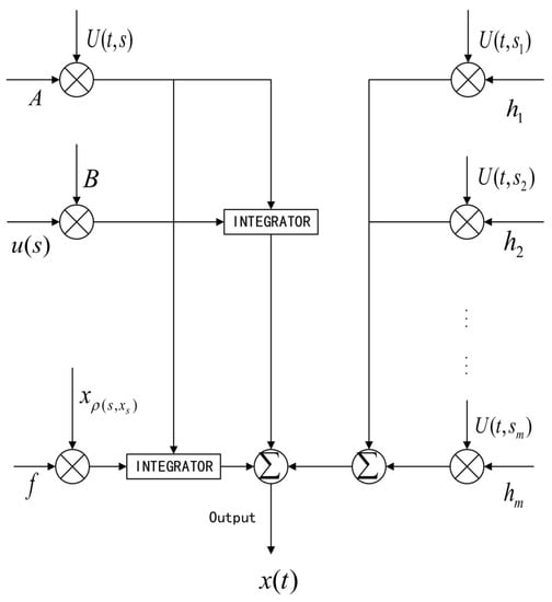
Figure 1. Filter system.

• Product modulator-1 accepts the input A and $U(t,s)$ produces the output as $AU(t,s)$.
• Product modulator-2 accepts the input B and $u\left(s\right)$ produces the output as $Bu\left(s\right)$.
• Product modulator-3 accepts the input f and $x_{\rho (s,x_s)}$ produces the output as $f(s,x_{\rho (s,x_s)})$.
• Here integrators performed the integral of $U(t,s)[f(s,x_{\rho (s,x_s)})+Bu\left(s\right)]$, over the period t.

In addition,

(i)

Inputs $U(t,s)$ and $f(s,x_{\rho (s,x_s)})$ are combined and multiplying with an output of integrator over $(0,t)$.

(ii)

Inputs $U(t,s)$ and $Bu\left(s\right)$ are combined and multiplying with an output of integrator over $(0,t).$

Lastly, we move all the outputs from the integrators to the summer network. Hence, our output of $x\left(t\right)$ is acquired, which is bounded and totally controllable.

References

- Arora, S.; Dabas, J. Existence and approximate controllability of non-autonomous functional impulsive evolution inclusions in Banach spaces. J. Differ. Equ. 2022, 307, 83–113. [Google Scholar] [CrossRef]
- Arora, S.; Dabas, J. Approximate controllability of the non-autonomous impulsive evolution equation with state-dependent delay in Banach spaces. Nonlinear Anal. Hybrid Syst. 2021, 39, 100989. [Google Scholar] [CrossRef]
- Li, Y.; Liu, Y. Multiple solutions for a class of boundary value problems of fractional differential equations with generalized Caputo derivatives. AIMS Math. 2021, 6, 1–24. [Google Scholar] [CrossRef]
- Liu, Y.; Liu, Y. Multiple positive solutions for a class of boundary value problem of fractional (p,q)-difference equations under (p,q)-integral boundary conditions. J. Math.-UK 2021, 13, 2969717. [Google Scholar] [CrossRef]
- Wouw, N.; Leine, R. Tracking control for a class of measure differential inclusions. In Proceedings of the 47th IEEE Conference on Decision and Control, Cancun, Mexico, 9–11 December 2008. [Google Scholar]
- Hernández, E.; O’regan, D. On a new class of abstract impulsive differential equations. Proc. Am. Math. Soc. 2013, 141, 1641–1649. [Google Scholar] [CrossRef] [Green Version]
- Wang, J.; Fěckan, M. Non-Instantaneous Impulsive Differential Equations; IOP: Bristol, UK, 2018. [Google Scholar]
- Borah, J.; Bora, S. Existence of mild solutions for a class of fractional non-autonomous evolution equations with delay. Fract. Calc. Appl. Anal. 2019, 22, 1–14. [Google Scholar] [CrossRef]
- Chalishajar, D.; Kumar, A. Total controllability of the second order semi-linear differential equation with infinite delay and non-instantaneous impulses. Math. Comput. Appl. 2018, 23, 32. [Google Scholar] [CrossRef] [Green Version]
- Kumar, S.; Mohammad, S. Approximate controllability of non-instantaneous impulsive semilinear measure driven control system with infinite delay via fundamental solution. IMA J. Math. Control Inf. 2020, 38, 552–575. [Google Scholar] [CrossRef]
- Wang, J.; Ibrahim, A.; Fečkan, M.; Zhou, Y. Controllability of fractional non-instantaneous impulsive differential inclusions without compactness. IMA J. Math. Control Inf. 2017, 36, 443–460. [Google Scholar] [CrossRef]
- Lygeros, J.; Tomlin, C. Hybrid Systems: Modeling, Analysis and Control; Tech. Rep. UCB/ERL M; Electronic Research Laboratory, University of California: Berkeley, CA, USA, 2008; Volume 99, p. 6. Available online: https://www.researchgate.net/publication/260082743 (accessed on 28 December 2008).
- Das, P.; Sharma, R. Existence and stability of measure differential equations. Czechoslovak. Math. J. 1972, 22, 145–158. [Google Scholar] [CrossRef]
- Pandit, S.; Deo, S. Differential Systems Involving Impulses; Springer: Berlin/Heidelberg, Germany, 1982. [Google Scholar]
- Satco, B. Regulated solutions for nonlinear measure driven equations. Nonlinear Anal. 2014, 13, 22–31. [Google Scholar] [CrossRef]
- Petrusel, A.; Satco, B. Semilinear evolution equations with distributed measures. Fixed. Point. Theory. Appl. 2015, 2015, 145. [Google Scholar] [CrossRef] [Green Version]
- Ravichandran, C.; Valliammal, N.; Nieto, J.J. New results on exact controllability of a class of fractional neutral integro-differential systems with state-dependent delay in Banach spaces. J. Frankl. Inst. 2020, 356, 1535–1565. [Google Scholar] [CrossRef]
- Vijayakumar, V.; Udhayakumar, R. Results on approximate controllability for non-densely defined Hilfer fractional differential system with infinite delay. Chaos Soliton Fract. 2020, 139, 110019. [Google Scholar] [CrossRef]
- Cao, Y.; Sun, J. Controllability of measure driven evolution systems with nonlocal conditions. Appl. Math. Comput. 2017, 299, 119–126. [Google Scholar] [CrossRef]
- Cao, Y.; Sun, J. Approximate controllability of semilinear measure driven systems. Math. Nachr. 2018, 291, 1979–1988. [Google Scholar] [CrossRef]
- Gou, H.; Li, Y. Existence and approximate controllability of semilinear measure driven systems with nonlocal conditions. Bull. Iran. Math. Soc. 2021, 48, 769–789. [Google Scholar] [CrossRef]
- Gu, H.; Sun, Y. Nonlocal controllability of fractional measure evolution equation. J. Inequal. Appl. 2020, 2020, 60. [Google Scholar] [CrossRef]
- Kumar, S.; Abdal, S.M. Approximate controllability of nonautonomous second-order nonlocal measure driven systems with state-dependent delay. Int. J. Control 2022, 2022, 1–12. [Google Scholar] [CrossRef]
- Wan, X.; Sun, J. Approximate controllability for abstract measure differential systems. Syst. Control Lett. 2012, 61, 50–54. [Google Scholar] [CrossRef]
- Sharma, R. An abstract measure differential equation. Proc. Am. Math. Soc. 1972, 32, 503–510. [Google Scholar] [CrossRef]
- Hino, Y. Functional Differential Equations with Infinite Delay; Springer: Berlin/Heidelberg, Germany, 1991. [Google Scholar]
- Leonov, G.; Nijmeijer, H. Dynamics and Control of Hybrid Mechanical Systems. In World Scientific Series on Nonlinear Science Series B; Singapore: World Scientific Publishing, 2010; Volume 14, Available online: https://www.worldscientific.com/worldscibooks/10.1142/7421 (accessed on 10 January 2010).
- Hale, J.; Kato, J. Phase space for retarded equations with infinite delay. Funk. Ekvac. 1978, 21, 11–41. [Google Scholar]
- Krasnosel’skii, M.A. Some problems of nonlinear analysis. In American Mathematical Society Translations, Ser. 2; American Mathematical Society: Providence, RI, USA, 1958; Volume 10, pp. 345–409. [Google Scholar]
- Subashini, R.; Jothimani, K.; Nisar, K.S.; Ravichandran, C. New results on nonlocal functional integrodifferential equations via Hilfer fractional derivative. Alex. Eng. J. 2020, 59, 2891–2899. [Google Scholar] [CrossRef]
Publisher’s Note: MDPI stays neutral with regard to jurisdictional claims in published maps and institutional affiliations. |
© 2022 by the authors. Licensee MDPI, Basel, Switzerland. This article is an open access article distributed under the terms and conditions of the Creative Commons Attribution (CC BY) license (https://creativecommons.org/licenses/by/4.0/).