Application of Smooth Fuzzy Model in Image Denoising and Edge Detection

Abstract

In this paper, the bounded variation property of fuzzy models with smooth compositions have been studied, and they have been compared with the standard fuzzy composition (e.g., min–max). Moreover, the contribution of the bounded variation of the smooth fuzzy model for the noise removal and edge preservation of the digital images has been investigated. Different simulations on the test images have been employed to verify the results. The performance index related to the detected edges of the smooth fuzzy models in the presence of both Gaussian and Impulse (also known as salt-and-pepper noise) noises of different densities has been found to be higher than the standard well-known fuzzy models (e.g., min–max composition), which demonstrates the efficiency of smooth compositions in comparison to the standard composition.

1. Introduction

Edge detection is a useful step toward visual object detection and image segmentation. An edge is normally extracted by the observation of the intensity changes inside the region of interest of the entire image. Therefore, different gradient calculation measures have been developed in the literature to find the abrupt changes of the pixel’s qualities. The Robert edge detection algorithm, as a basic method of edge detection, calculates the discrete differentiation between the diagonally adjacent pixels [1,2]. Similarly, Sobel edge detection and Prewitt edge detection perform the same process of differentiation inside the horizontal and vertical masks, respectively. Canny edge detection is considered as the standard edge detection technique, where the process is performed in three stages. Firstly, the image goes through the Gaussian filter to be smoothed. Secondly, the directional gradient is calculated to estimate the edges. The third step is the post-processing, where it is attempted to thin the edges [3]. The smoothing of the image is also used in the other well-established algorithms of edge detection, such as Laplacian of Gaussian (LoG), where the sum of the second derivative of the Gaussian function is used [4]. However, the variation of the pixel values across the region of interest and the induced noises during the recording and transformation can degenerate the image detection process. Readers interested in a survey of the mentioned algorithms are referred to [1,5,6].

The wider applications of the image processing algorithms in industry, robotics, military, geography, and medical diagnosis detection have acted as a motor for the development of the recent algorithms in the image segmentation [7,8,9], morphological operations [3], and noise removal [10]. The basic edge detection algorithms have been highly extended in recent years. For instance, for the better smoothing of images, the geometry of images has been used upon the bandlet transformation to improve the performance of edge detection algorithms in [11]. The Faber Shcauder wavelet transformation has been used with a bilateral filtering method in [12]. Many research works also have been performed to tackle the noise reduction problem in edge detection.

Normally, it is impossible to identify the kind or level of noise in an image; however, it is believed that the impulse (type) noises are more related to the image acquisition process (i.e., scanning and motion blurring) and the Gaussian (type) noises are related to the transmission process. Hence, many researchers have focused on soft computing methods and fuzzy models for the development of the robust algorithms of the edge detection of the noisy images [5,13,14]. Soft computing methods and fuzzy models, in general, can incorporate more parameters and different high-pass or low-pass filters into the edge detection algorithm and therefore preserve the edges while simultaneously smoothing the noises [1].

Several applications of the standard fuzzy logic-based edge detection have been reported in the literature. In [1], the type-2 fuzzy model has been employed. The anisotropic filtering has been developed in [15]. In [16], a modified region growing procedure is introduced to evaluate the distance between a pixel and the region. However, the shortages of the fuzzy models in general are as follows:

• Although it is proved that the fuzzy models can approximate any continuous function in the compact set, their derivative is not continuous. In other words, the fuzzy models are not smooth [17].
• The type-2 fuzzy logics improve the performance of the edge detection algorithms; however, they demand higher computational power in parallel.
• The selection of the best shape of membership function (MF) is mostly a problematic matter in the design step, and many developed methods are only applicable to a special shape of MF.

Therefore, in the present manuscript, we intend to employ the smooth fuzzy compositions (SFCs) for edge detection and noise removal purposes. The novelties and contributions of the proposed method are as follows:

• The fuzzy models with smooth compositions are classified as type-1 fuzzy models. Therefore, they do not call for notably higher computational power compared to the standard fuzzy models of min–max and product–sum compositions.
• Considering the structural properties, the smooth fuzzy models (SFMs) are bounded variation functions, enabling them to dampen the noises in the image, even at low signal-to-noise ratios (SNRs).
• The results for the bounded variation property are general for all MF selections.

The bounded variation property of the smooth compositions is the backbone of the proposed approach in the manuscript, and we have compared the total variation denoising of the smooth fuzzy compositions to the standard fuzzy compositions through quantitative methods. Upon this characteristic, therefore, the smooth fuzzy models would preserve the edges and important information of the images. This capacity has been demonstrated through the comparison of Pratt’s figure of merit (PFOM) values of the different models.

Two cases of Gaussian noise and Impulse noise have been considered in the simulations. Considering that the source and type of the noises usually are not determined, and the proposed method is able to remove both types of noises, the results are highly applicable to real applications.

Therefore, the structure of the manuscript is as follows. We begin with the preliminaries of the functional analysis and then introduce the general fuzzy modeling and the smooth fuzzy modeling schemes. In the next section, we elaborate on the bounded variation property of the smooth fuzzy compositions and contrast the total variation denoising of the smooth fuzzy compositions toward the standard fuzzy compositions. After that, we employ the obtained results for the edge detection of the images and demonstrate the higher performance of the smooth compositions over the standard fuzzy compositions for the edge detection. Finally, the results are discussed, and the paper is concluded.

2. Preliminaries

2.1. Mathematical Background

In this section, for the convenience of the reader, we review some mathematical backgrounds from [17].

Definition 1.

A function $\psi :[a,b]\to R$ is Lipschitz if there is a constant $c\ge 0$ such that for all $u,v\in [a,b],\left|f\right(u)-f(v\left)\right|\le c|u-v|$. The infimum of such c is called the Lipschitz constant.

Proposition 1.

If ψ is differentiable on $(a,b)$ and its derivative ${\psi }^{\prime }$ is increasing, then ψ is convex.

Proposition 2.

Let ψ be a convex function on $(a,b)$. ψ is then Lipschitz, and thus absolutely continuous, on each closed, bounded subinterval $[c,d]$ of $(a,b)$.

Lemma 1.

Let the function ψ be absolutely continuous on the closed, bounded interval $[a,b]$. Then, f is the difference of increasing absolutely continuous functions and, in particular, is of bounded variation.

Proof of Lemma 1. 

See [17]. □

2.2. General Structure of Fuzzy Systems

After reviewing the mathematical preliminaries from [17], we continue to the main part of the manuscript.

We consider a system of multiple inputs and single output to facilitate the theory development; however, it is clear to us that our results can be extended for multiple input–multiple output systems since the multiple output part can be easily decomposed into several single outputs of the system.

We consider a system where the state depends on the last n states of the system as follows:

$$\begin{array}{cc}\hfill & h:R^n\to R,\hfill \end{array}$$

(1)

$$\begin{array}{cc}\hfill & x(k+1)=h\left(x\left(k\right),x(k-1),\dots ,x(k-n+1)\right).\hfill \end{array}$$

(2)

We call every i-th past state of the system state $x_i$; hence, the system definition changes to be as follows:

$$x(k+1)=h(x_1,x_2,\dots ,x_n).$$

(3)

For every state of the system, we consider an interval where each state has the highest probability of existence in that interval. Hence, we partition the interval into $2N+1$ regions and assign an MF for each region.

To complete the fuzzy system definition, we need to assign rules for the data in each region of domain of the inputs and outputs. In mathematical terms, we consider the following:

$$R^{\left(i\right)}:\mathrm{If} x_1 \mathrm{is} M_1^i \mathrm{and} x_2 \mathrm{is} M_2^i \mathrm{and}\dots \mathrm{and} x_n \mathrm{is} M_n^i, \mathrm{then} g\left(x\right) \mathrm{is} d_i \mathrm{under} \mathrm{the} \mathrm{possibility} {\mu }_i\left(x\right),i=1,\dots ,r,$$

(4)

where the function $x(k+1):=g\left(x\right)$, $x=[x_1,\dots ,x_n]$, $0\in x$ is about to approximate the system dynamics $h\left(x\right)$ in the corresponding interval. The fuzzy rules we have just constructed are supposed to have two IF and THEN parts, which can be interpreted to make a mathematical inference based on the fuzzy values employing the compositions of t-norms and s-norms.

Different types of t-norms and s-norms have been introduced in the literature [18,19,20], where the min–max composition and product–sum composition are the mostly used compositions and are shown as follows:

$$\mathrm{I}:\{\begin{array}{}\mathrm{(5a)}& T(a,b)=\min a,b,\mathrm{(5b)}& S(a,b)=\max a,b,\end{array}$$

$$\mathrm{II}:\{\begin{array}{}\mathrm{(6a)}& T(a,b)=a·b,\mathrm{(6b)}& S(a,b)=a+b-a·b\end{array}$$

We consider that the output of a fuzzy model is determined upon the centroid defuzzification formula, given by

$$x(k+1):=g\left(x\right)=\frac{{\sum }_{i=1}^r{d}_i·{\mu }_i\left(x\right)}{{\sum }_{i=1}^r{\mu }_i\left(x\right)}.$$

(7)

2.3. Smooth Fuzzy Models

In [18,21,22,23], the smooth fuzzy models are generally constructed upon the utilization of SFCs instead of the standard fuzzy compositions introduced above. The SFCs are smooth t-norms and smooth s-norms, and are shown as follows:

$$\mathrm{I}:\{\begin{array}{}\mathrm{(8a)}& T_A(a,b)=1-\cos (\frac{2}{\pi }{\cos }^{-1}(1-a){\cos }^{-1}(1-b)),\mathrm{(8b)}& S_A(a,b)=\frac{v·\omega ·{\beta }^{-{\log }_{\beta }(v){\log }_{\beta }(\omega )}-1}{\beta -1},\end{array}$$

where $\beta \in (1,\infty )$, $(\beta -1)a+1$, and $\varpi =(\beta -1)b+1$;

$$\mathrm{II}:\{\begin{array}{}\mathrm{(9a)}& T_B(a,b)=\frac{4}{\pi }{\tan }^{-1}(\tan (\frac{\pi }{4}a)\tan (\frac{\pi }{4}b)),\mathrm{(9b)}& S_B(a,b)=1-\frac{4}{\pi }{\tan }^{-1}(\tan (\frac{\pi }{4}(1-a))\tan (\frac{\pi }{4}(1-b))),\end{array}$$

$$\mathrm{III}:\{\begin{array}{}\mathrm{(10a)}& T_C(a,b)=1-\frac{2}{\pi }{\cos }^{-1}(\sin (\frac{\pi }{2}a)\sin (\frac{\pi }{2}b)),\mathrm{(10b)}& S_C(a,b)=\frac{2}{\pi }{\cos }^{-1}(\cos (\frac{\pi }{2}a)\cos (\frac{\pi }{2}b)),\end{array}$$

$$\mathrm{IV}:\{\begin{array}{}\mathrm{(11a)}& T_D(a,b)=\cos ({\cos }^{-1}(a)+{\cos }^{-1}(b)-\frac{2}{\pi }{\cos }^{-1}(a){\cos }^{-1}(b)),\mathrm{(11b)}& S_D(a,b)=\cos (\frac{2}{\pi }{\cos }^{-1}(a){\cos }^{-1}(b)).\end{array}$$

To facilitate the explanation, we assume $r=2$, corresponding to the MFs ${\mu }_a\left(x\right)$ and ${\mu }_b\left(x\right)$, along with two state variables. Then, the fuzzy model can be written as follows:

$$g\left(x\right)=\frac{d_1·{\mu }_1\left(x\right)+d_2·{\mu }_2\left(x\right)}{{\mu }_1\left(x\right)+{\mu }_2\left(x\right)},$$

(12)

where ${\mu }_1\left(x\right)$ and ${\mu }_2\left(x\right)$ are the MFs from the system state vector $x={\left[x_1{x}_2\right]}^T$.

$${\mu }_i\left(x_i\right)=S\left(T\left({\mu }_a\left(x_i\right),{\mu }_b\left(x_i\right)\right)\right),i=1,2.$$

(13)

For more details on such calculations, interested readers are referred to [23,24,25,26,27,28,29,30,31,32].

Lemma 2.

The composition of smooth fuzzy operators class B is Lipschitz with respect to the MF.

Proof of Lemma 2. 

To prove the lemma, we must check that the derivatives of the s–t composition class B with respect to MF are increasing in the interval $[0,1]$. Hence, based upon Propositions 1 and 2, the proof is complete. □

For two MFs ${\mu }_a\left(x\right)$ and ${\mu }_b\left(x\right)$, we define B as follows:

$$B=S_B\left(T_B\left({\mu }_a(·),{\mu }_b(·)\right)\right).$$

(14)

Therefore, the derivative using the chain rule will be as follows:

$$\begin{array}{cc}\hfill B^{\prime }& =S_B^{\prime }\left(T_B\left({\mu }_a(·),{\mu }_b(·)\right)\right)\times T_B^{\prime }\left({\mu }_a(·),{\mu }_b(·)\right)\hfill \\ \hfill & =\frac{\frac{\pi }{4}\left(\frac{\pi }{4}{sec}^2\left(\frac{\pi }{4}{\mu }_j(·)\right)\right)}{1+{\left(tan\left(\frac{\pi }{4}{\mu }_a(·)\right)tan\left(\frac{\pi }{4}{\mu }_b(·)\right)\right)}^2}\times \frac{\frac{-\pi }{4}\left(\frac{-\pi }{4}{sec}^2\left(\frac{\pi }{4}\left(1-{\mu }_j(·)\right)\right)\right)}{1+{\left(tan\left(\frac{\pi }{4}\left(1-{\mu }_a(·)\right)\right)tan\left(\frac{\pi }{4}\left(1-{\mu }_b(·)\right)\right)\right)}^2},\hfill \end{array}$$

(15)

and $B^{\prime }\ge 0$, $j=a,b$.

Corollary 1.

The s–t smooth composition class B is absolutely continuous.

Proof of Corollary 1. 

Corollary 1 can be deduced from Lemma 2, Propositions 1 and 2. □

Theorem 1.

The s–t smooth composition class B is a bounded variation function.

Proof of Theorem 1. 

Theorem 1 can be deduced from Corollary 1 and Lemma 1. □

3. Comparison of Bounded Variation of Different Fuzzy Compositions

The functions of the bounded variations property have been studied widely in the literature [17,33,34,35,36,37,38], and many researchers have worked on their applications for edge preservation and noise reduction. In the previous section, we concluded that the smooth compositions are bounded variation functions of MF. Hence, in this section, we demonstrate what the bounded variation property means for the smooth fuzzy compositions and quantify the noise removal capacity of different fuzzy compositions. We employ the PFOM as the instrument for this purpose.

3.1. Instrumentation (Pratt’s Figure of Merit)

Pratt in [39,40] introduced a figure of merit as an index for errors in edge detection as follows:

$$\mathrm{PFOM}=\frac{1}{max(I_I,I_A)}\sum _{k=1}^{I_A}\frac{1}{1+\alpha d^2\left(k\right)},$$

(16)

where $I_I$ is the number of ideal edge points, $I_A$ is the number of actual or detected edge points, $\alpha$ is a scaling constant (typically equal to $1/9$), and d is the separation distance of the actual edge point normal to the line of ideal edge points. In the literature [5,41,42,43,44], various approaches are provided to compute distance d. Some possible definitions of distance, which compute the distance between the position of two pixels $(v_1,w_1)$ and $(v_2,w_2)$, are as follows:

• City block distance, based on four-connectivity, provides only horizontal and vertical distances for movements:

  $$d_{cit}=|v_1-v_2|+|w_1-w_2|.$$

  (17)
• Chessboard distance, based on eight-connectivity, provides diagonal distances for movements as well as horizontal and vertical distances for movements:

  $$d_{chess}=max\left(|v_1-v_2|,|w_1-w_2|\right).$$

  (18)
• Euclidean distance measures the actual physical distance as

  $$d_{euc}=\sqrt{{(v_1-v_2)}^2+{(w_1-w_2)}^2}.$$

  (19)

3.2. Illustrations

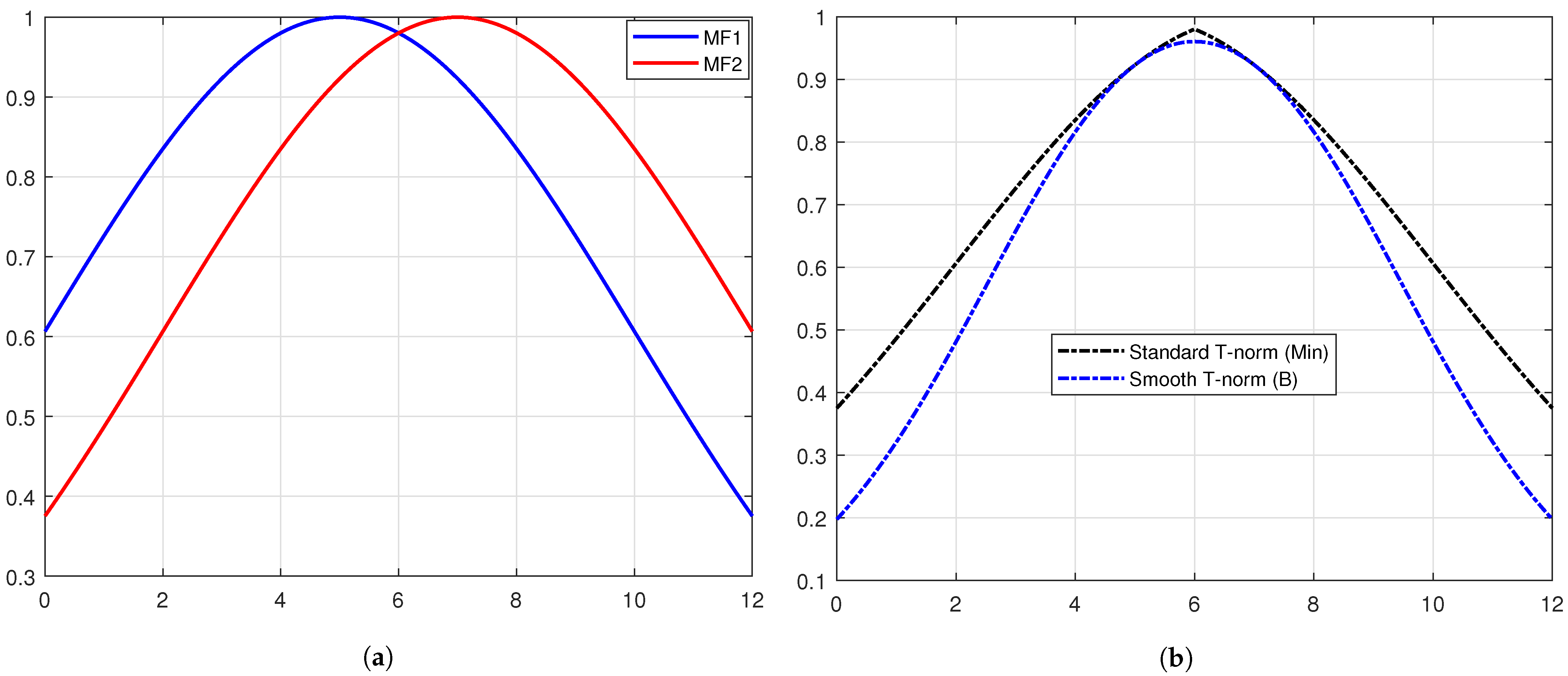
In this section, we consider the “Euclidean distance” between MFs and compare the performance of the different t-norm operators. Two MFs of the Gaussian shapes are considered as follows:

$$\{\begin{array}{}\mathrm{(20a)}& {MF}_1=Gaussian(m_1,{std}_1\hspace{1em}{m}_1=5 and {std}_1=5,\mathrm{(20b)}& {MF}_2=Gaussian(m_2,{std}_2\hspace{1em}{m}_2=7 and {std}_2=5.\end{array}$$

The outputs of different t-norm operators have been studied with these MFs. The t-norm operators in the study are (i) the smooth fuzzy t-norm type B and (ii) the standard fuzzy t-norm min. As has been shown in Figure 1, the performance of the two t-norm operators is the same under the normal condition. Now, we consider the noisy conditions.

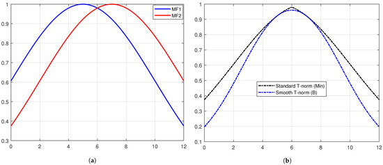
Figure 1. Performance of different t-norm operators under normal condition. (a) Membership Functions. (b) Output of Fuzzy T-norms.

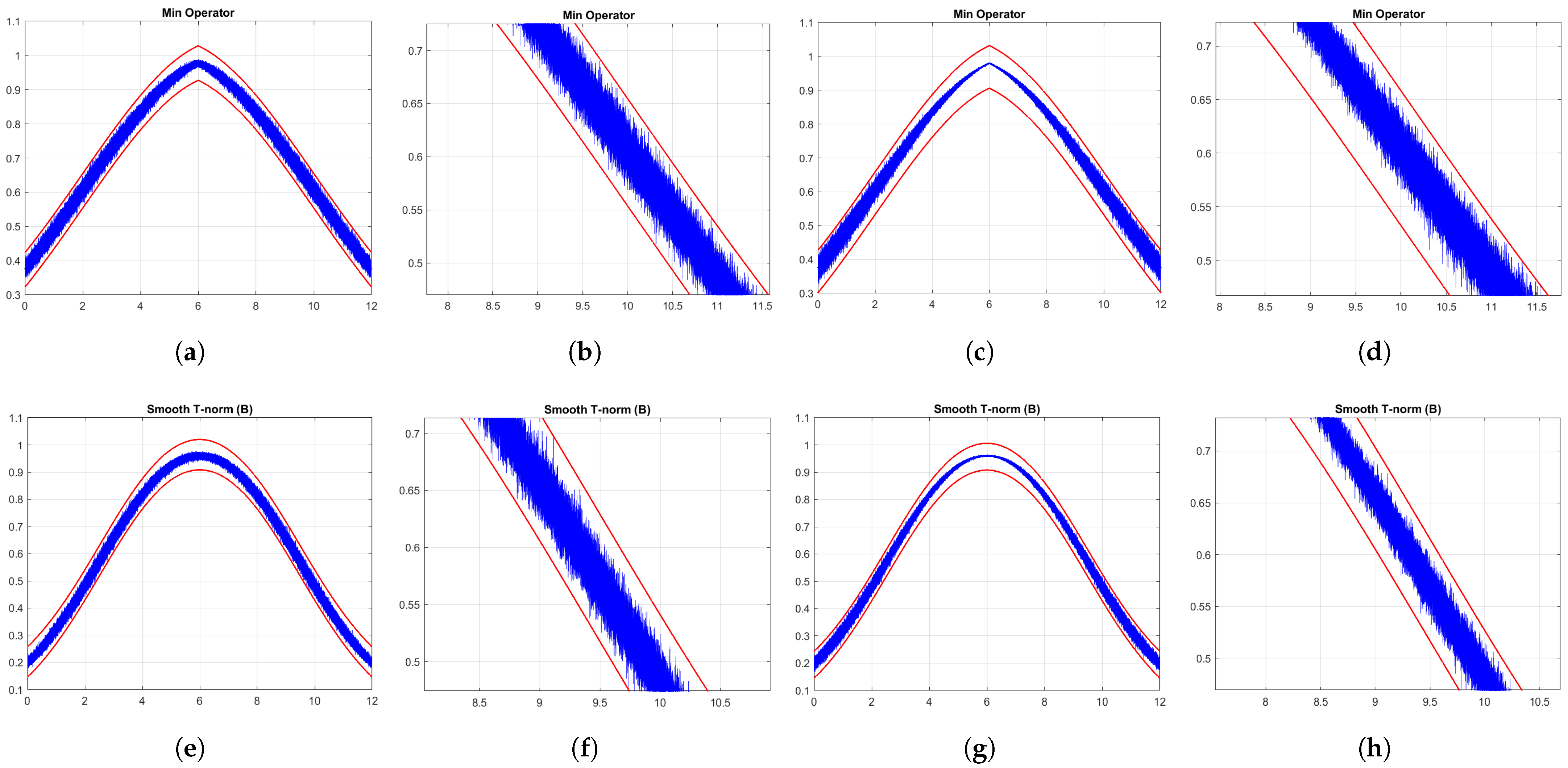
• Scenario 1: Both MFs are considered with additive noise as follows:

  $$\begin{array}{cc}\hfill {\tilde{m}}_1& \hfill =m_1+noise,\hfill \end{array}$$

  (21)

  $$\begin{array}{cc}\hfill {\tilde{m}}_2& \hfill =m_2+noise.\hfill \end{array}$$

  (22)

  Therefore, the MFs can be considered as follows:

  $$\begin{array}{cc}\hfill M{F}_1& \hfill =Gaussian({\tilde{m}}_1,st{d}_1),\hfill \end{array}$$

  (23)

  $$\begin{array}{cc}\hfill M{F}_2& \hfill =Gaussian({\tilde{m}}_2,st{d}_2).\hfill \end{array}$$

  (24)

  The impacts of the two t-norm operators are different, as illustrated in Figure 2.
  

  Figure 2. Impacts of different t-norm operators. (a) $m+noise$. (b) Zoomed in. (c) $std+noise$. (d) Zoomed in. (e) $m+noise$. (f) Zoomed in. (g) $std+noise$. (h) Zoomed in.
• Scenario 2: Both MFs are considered with the additive noise as follows:

  $$\begin{array}{cc}\hfill {\widetilde{std}}_1& \hfill =st{d}_1+noise,\hfill \end{array}$$

  (25)

  $$\begin{array}{cc}\hfill {\widetilde{std}}_2& \hfill =st{d}_2+noise.\hfill \end{array}$$

  (26)

  Therefore, the MFs can be considered as follows:

  $$\begin{array}{cc}\hfill M{F}_1& \hfill =Gaussian(m_1,{\widetilde{std}}_1),\hfill \end{array}$$

  (27)

  $$\begin{array}{cc}\hfill M{F}_2& \hfill =Gaussian(m_2,{\widetilde{std}}_2).\hfill \end{array}$$

  (28)

  The impacts of the two t-norm operators are different, as illustrated in Figure 2.

It is evident from the comparison of the PFOM corresponding to the different t-norm operators, summarized in Table 1 and Table 2, that the smooth operator shows a higher level of tolerance to the noises.

Table 1. PFOM-based comparison of the T-norm operators with additive noise to the mean of the MFs.

$\mathit{\alpha }$-Plane	Min Operator	Smooth T-Norm (B)
$0.5$	$93.95\%$	$95.65\%$
$0.7$	$93.82\%$	$94.93\%$

Table 2. PFOM-based comparison of the T-norm operators with additive noise to the standard deviation of the MFs.

$\mathit{\alpha }$-Plane	Min Operator	Smooth T-Norm (B)
$0.5$	$92.21\%$	$96.16\%$
$0.7$	$94.37\%$	$96.89\%$

4. Application to Edge Detection of Images

In this section, we verify how the employment of smooth fuzzy compositions removes noises and preserves the edges of the images. In the previous section, it was demonstrated that smooth fuzzy compositions outperformed the standard fuzzy compositions in dampening the effect of the noises. Therefore, for the edge detection of images, the application of the smooth compositions has been compared to the standard fuzzy compositions, and to make a fair comparison, the same structure of the fuzzy model has been considered for both types of compositions.

4.1. Non-Fuzzy Edge Detection

In the classical edge detection algorithm, the Sobel operators are employed as the vertical and horizontal derivative approximations of the image. The algorithm employs Sobel operators throughout the horizontal axis and vertical axis, as follows:

$$\begin{array}{cc}{H}_{horiz}=\left[\begin{array}{ccc}-1& 0& +1\\ -2& 0& +2\\ -1& 0& +1\end{array}\right],& H_{vert}=\left[\begin{array}{ccc}+1& +2& +1\\ 0& 0& 0\\ -1& -2& -1\end{array}\right],\end{array}$$

which act as three-by-three convolution masks on the image. Therefore, the gradients along both axes are determined as follows:

$$\{\begin{array}{}\mathrm{(29a)}& h_{horiz}=H_{horiz}\ast IMG,\mathrm{(29b)}& h_{vert}=H_{vert}\ast IMG.\end{array}$$

where ∗ represents the convolution operator. It is attempted to detect the zero-crossings of the first-order directional derivative in the gradient direction of the image by the minimization of the following function:

$$h=\sqrt{h_{horiz}^2+h_{vert}^2}.$$

(30)

4.2. Fuzzy Edge Detection

For the fuzzy edge detection algorithm, we consider four inputs to the fuzzy system. The first two inputs are the vertical and horizontal derivative approximations of the image, $h_{horiz}$ and $h_{vert}$, respectively. The third input to the fuzzy system is the output of the image through a convolution mask of a low-pass filter, which is as follows:

$$\begin{array}{c}LP=\frac{1}{25}\left[\begin{array}{ccccc}1& 1& 1& 1& 1\\ 1& 1& 1& 1& 1\\ 1& 1& 1& 1& 1\\ 1& 1& 1& 1& 1\\ 1& 1& 1& 1& 1\end{array}\right],\end{array}$$

$$lp=LP\ast IMG.$$

(31)

The fourth input to the fuzzy system is the output of a convolution mask of a high-pass filter, which is as follows:

$$\begin{array}{c}HP=\left[\begin{array}{ccc}-\frac{1}{16}& -\frac{1}{8}& -\frac{1}{16}\\ -\frac{1}{8}& +\frac{3}{4}& -\frac{1}{8}\\ -\frac{1}{16}& -\frac{1}{8}& -\frac{1}{16}\end{array}\right],\end{array}$$

$$hp=HP\ast IMG.$$

(32)

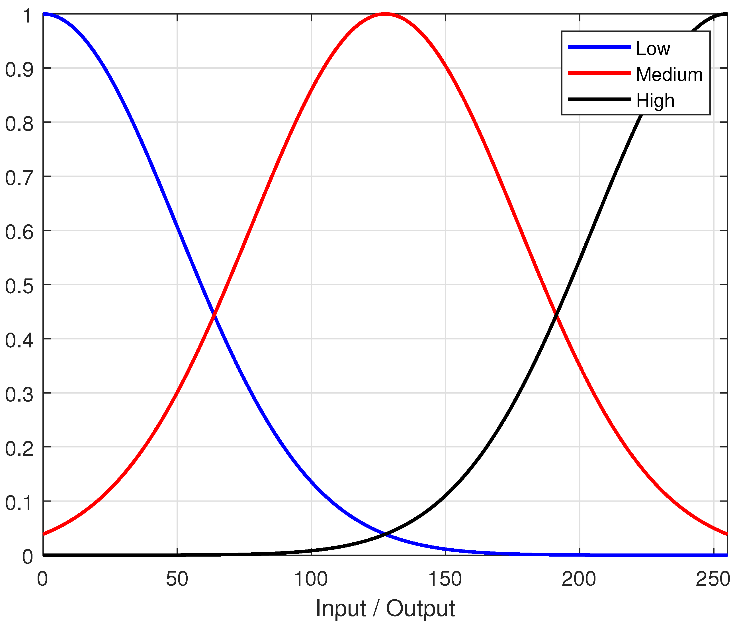
Consequently, the fuzzy model $g\left(x\right)$ can be constructed upon the suitable synchronization of the rules on the inputs. The rule basis for this fuzzy system is shown in Table 3. The MFs for all the inputs and the output are shown in Figure 3. The range on which the MFs are defined is flexible for the inputs and can extend further than 255 or lower than 0. However, the range of MF is fixed for the output, $[0,255]$.

Table 3. The Rule Base for the Fuzzy System.

Rule Number	Rule Definition
1	If $h_{horiz}$ is Low and $h_{vert}$ is Low, then output is Low.
2	If $h_{horiz}$ is Medium and $h_{vert}$ is Medium, then output is High.
3	If $h_{horiz}$ is High and $h_{vert}$ is High, then output is High.
4	If $lp$ is Low and $h_{vert}$ is Medium, then output is Low.
5	If $lp$ is Low and $h_{horiz}$ is Medium, then output is Low.
6	If $hp$ is Low and $h_{vert}$ is Medium, then output is High.
7	If $hp$ is Low and $h_{horiz}$ is Medium, then output is High.

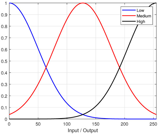
Figure 3. The MFs of all the inputs and the output.

The fuzzy model detects the edges of the image in the range from 0 to 255. It is known that in the grayscale format, 255 corresponds to white and 0 means black, and therefore, the closer a pixel is to 255, the greater the probability of the pixel being identified as an edge pixel. Figure 4 illustrates the developed fuzzy inference system for this paper.

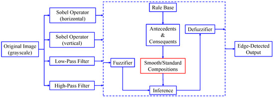
Figure 4. Fuzzy inference system.

Therefore, very similar to (30), the zero-crossings detection of the image can be carried out through the minimization of the first-order derivative of the fuzzy model as follows:

$$\left|\right|g\left(x\right)\left|\right|=\sum _{i=1}^r\sqrt{{\left(g_{horiz}^2\right)}_i+{\left(g_{vert}^2\right)}_i}.$$

(33)

The numerical solution of the minimization problem (33) is equal to the minimization of the norm function $\left|\right|g\left|\right|$ over the bounded variation search space of the image $\mathsf{\Omega }$, rewritten as follows:

$${argmin\left|\right|g\left(x\right)\left|\right|}_{g\left(x\right)\in BV\left(\mathsf{\Omega }\right)}=\sum _{i=1}^r\sqrt{{\left(g_{horiz}^2\right)}_i+{\left(g_{vert}^2\right)}_i}.$$

(34)

4.3. Noise Removal Characteristics of the Smooth Fuzzy Model

We consider the noisy image $f\left(x\right)$ as the output of the fuzzy model designed for the edge detection, added to the independently and identically distributed zero-mean Gaussian random variable $\eta$, as $f\left(x\right)=g\left(x\right)+\eta$. We amplify the minimization problem (34) to estimate the denoised image $g\left(x\right)$ as the solution of the following problem:

$$argmin\left({\int }_{\mathsf{\Omega }}{\left|\right|g\left(x\right)\left|\right|}_{g\left(x\right)\in BV\left(\mathsf{\Omega }\right)}\mathrm{d}x+\frac{\lambda }{2}{\int }_{\mathsf{\Omega }}{\left(f\left(x\right)-g\left(x\right)\right)}^2\mathrm{d}x\right),$$

(35)

where $\lambda$ is a positive parameter. The first term in the minimization avoids the solution from the oscillation behavior in the edge detection and smooths the images. The second term runs the smooth fuzzy model to remove the noise and to be close to the edges.

Lemma 3.

The solution of the minimization problem (35) exists and is unique and stable with respect to the perturbations.

Proof of Lemma 3. 

See [45]. □

Proposition 3.

The same conclusions of the noise-removing capacity of the smooth fuzzy models can be deduced for the definition of the Laplace noise and the minimization problem shown below:

$$argmin\left({\int }_{\mathsf{\Omega }}{\left|\right|g\left(x\right)\left|\right|}_{g\left(x\right)\in BV\left(\mathsf{\Omega }\right)}\mathrm{d}x+\frac{\lambda }{2}{\int }_{\mathsf{\Omega }}\left|\right|f\left(x\right)-g\left(x\right)\left|\right|\mathrm{d}x\right).$$

(36)

Proof of Proposition 3. 

See [46,47]. □

Proposition 4.

The same conclusions of the noise-removing capacity of the smooth fuzzy models can be deduced for the definition of the Poisson noise and the minimization problem shown below:

$$argmin\left({\int }_{\mathsf{\Omega }}{\left|\right|g\left(x\right)\left|\right|}_{g\left(x\right)\in BV\left(\mathsf{\Omega }\right)}\mathrm{d}x+\frac{\lambda }{2}{\int }_{\mathsf{\Omega }}{\left(f\left(x\right)log\left(g\right(x\left)\right)-g\left(x\right)\right)}^2\mathrm{d}x\right).$$

(37)

Proof of Proposition 4. 

See [48]. □

4.4. The Proposed Procedure

The grayscale image is used as the input to the fuzzy model of the edge detector system. Canny is used as the ideal edge detector for comparison using the PFOM value. A threshold filter is applied to the output image of the fuzzy model (fuzzy inference system) in such a way that the pixels with values higher than the threshold can be considered as the edge pixels (with pixel value being equal to 255), and the rest are considered as the non-edges (with a pixel value equal to 0). This process is called binarization.

In fact, in the binarization process, the threshold value for each image is selected adaptively. The output of the fuzzy inference system is a denoised gray-scale image with the edge pixels being more discernible than those of the input. Since the output pixels have values between 0 and 255, the threshold value will be a value in this range that provides the maximum PFOM in comparison with the ideal edge-detected image. In other words, a loop sweeps the interval of $[0,255]$ and selects the value that maximizes the PFOM. Finally, the edge-detected image pixel values will be either 0 or 255, which is called binarization. The employed procedure is illustrated in Algorithm 1 and Figure 5.

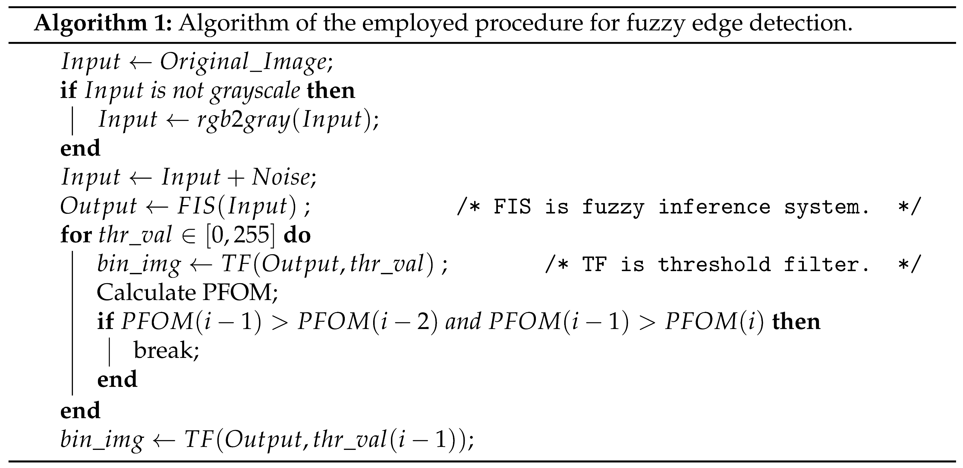
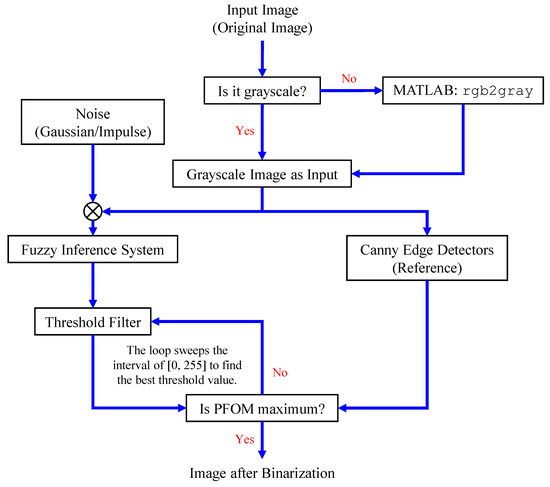
Figure 5. Flowchart of the employed procedure for fuzzy edge detection.

4.5. Comparison Instrument

Before proceeding to the edge detection, we need to choose the most fitted measure of distance, according to Section 3.1. The difference of the distance measures has been illustrated by the numerical comparison of an example in Figure 6, in which the pixel “aa” is located at $(2,1)$ and the pixel “bb” is located at $(3,3)$. The measures introduced above are used for the calculation of distance between the pixels as follows:

$$\begin{array}{cc}\hfill d_{cit}& =|2-3|+|1-3|=3\hfill \\ \hfill d_{chess}& =max\left(|2-3|,|1-3|\right)=2\hfill \\ \hfill d_{euc}& =\sqrt{{(2-3)}^2+{(1-3)}^2}=\sqrt{5}=2.236\hfill \end{array}$$

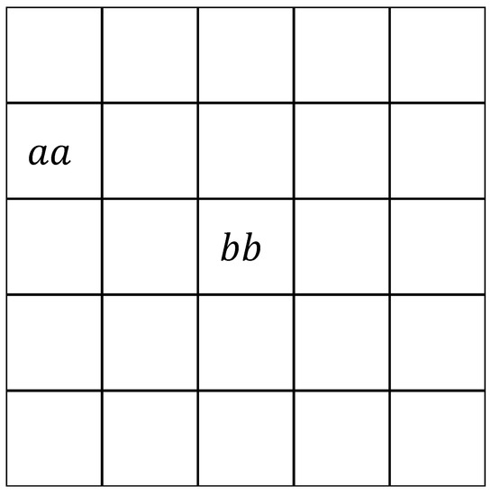
Figure 6. Example image for calculating the distance by various measures.

The “Euclidean distance” is based on the actual physical distance; however, the “Chessboard distance” can demonstrate movement in eight directions, which are almost all possible movements in an image. Secondly, with the employment of the “Chessboard distance,” the detected edges would have the same probability of belonging to the ideal edges.

5. Results and Discussions

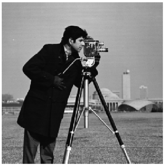
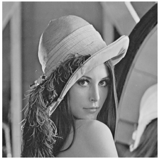
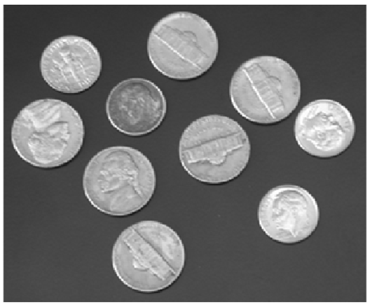
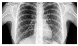
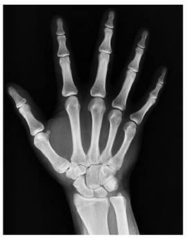
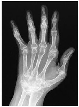
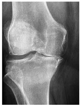
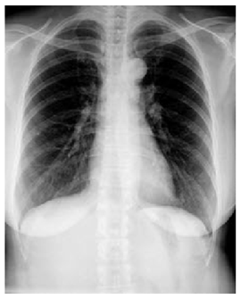
For the purpose of simulation, we consider two sets of images: (1) three images from MATLAB repository (Table 4) and (2) five X-ray images available online (Table 5).

Table 4. MATLAB Images.

Cameraman	Lena	Coins

Table 5. X-ray Images.

X-ray 1	X-ray 2	X-ray 3	X-ray 4	X-ray 5

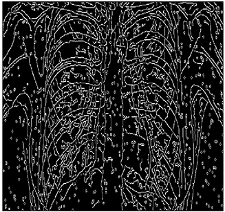
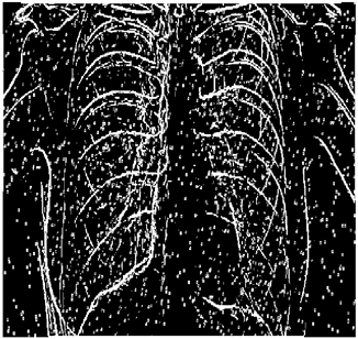
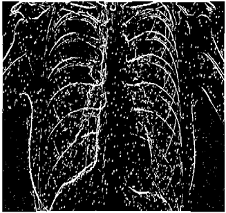
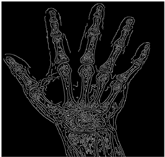
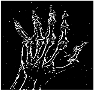
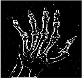
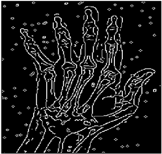
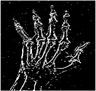
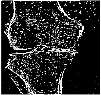
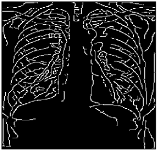
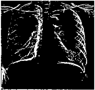
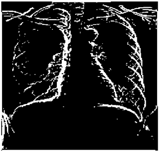
In Table 6, we show the results for applying the proposed method on each of the images and calculating the PFOM value under two types of noise: Gaussian and Impulse. Note that in these tables, the Gaussian noise is denoted by “G” with three different variance levels: $0.001$, $0.002$, and $0.003$. Similarly, the Impulse noise is denoted by “I” with three different density levels: $0.25\%$, $0.50\%$, and $1\%$.

Table 6. PFOM-based comparison of standard composition and smooth composition under different types of noise.

Image	Composition	No Noise	G(0.001)	G(0.002)	G(0.003)	I(0.25%)	I(0.5%)	I(1%)
Cameraman	Standard	0.9159	0.8987	0.8480	0.7881	0.8902	0.8796	0.8796
	Smooth	0.9256	0.9192	0.8841	0.8293	0.9009	0.8862	0.8867
Lena	Standard	0.9191	0.8905	0.8246	0.7951	0.8994	0.8715	0.8566
	Smooth	0.9266	0.9006	0.8530	0.8174	0.9052	0.8767	0.8642
Coins	Standard	0.9066	0.9025	0.8881	0.8448	0.9011	0.8943	0.8856
	Smooth	0.9294	0.9231	0.9180	0.8910	0.9284	0.9239	0.9211
X-ray 1	Standard	0.9207	0.8657	0.8303	0.8281	0.9113	0.9075	0.9010
	Smooth	0.9231	0.8758	0.8389	0.8338	0.9151	0.9109	0.9053
X-ray 2	Standard	0.8960	0.8653	0.8740	0.8304	0.9001	0.8967	0.8973
	Smooth	0.9051	0.8925	0.8879	0.8830	0.9045	0.9024	0.8974
X-ray 3	Standard	0.8998	0.8848	0.8690	0.8594	0.8922	0.8886	0.8725
	Smooth	0.9189	0.9084	0.8980	0.8891	0.9112	0.9052	0.8855
X-ray 4	Standard	0.8601	0.8556	0.8401	0.8537	0.8529	0.8635	0.8609
	Smooth	0.8737	0.8667	0.8546	0.8627	0.8710	0.8803	0.8791
X-ray 5	Standard	0.8784	0.8311	0.7501	0.7201	0.8748	0.8776	0.8788
	Smooth	0.8853	0.8397	0.7611	0.7309	0.8806	0.8842	0.8843

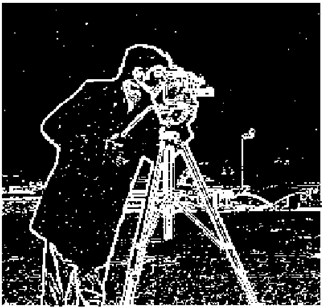
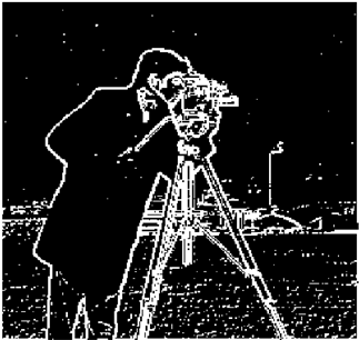
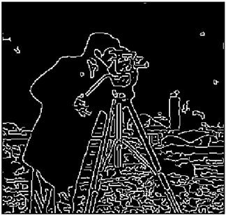
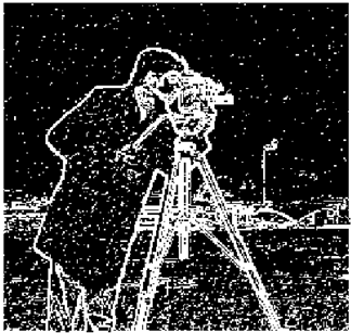
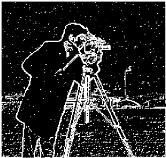
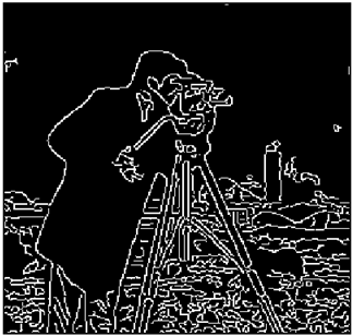
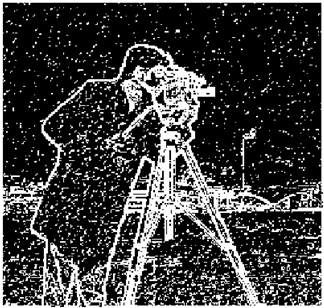
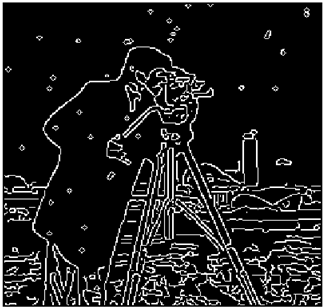
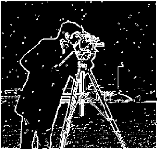
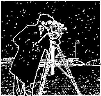
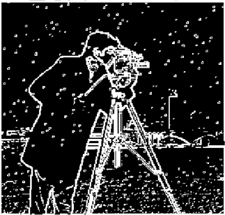
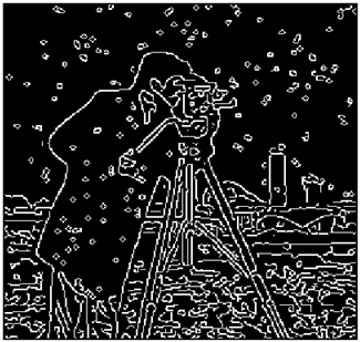
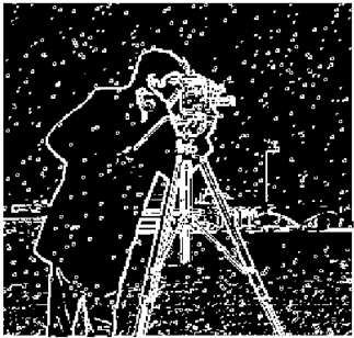
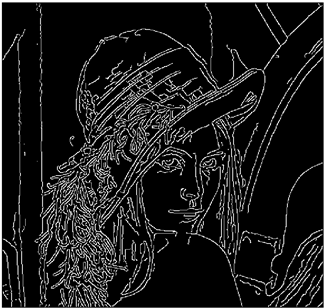
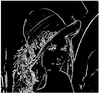
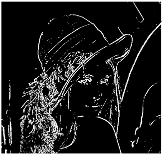
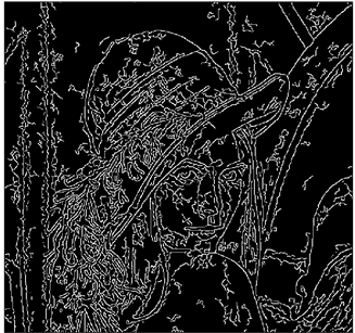
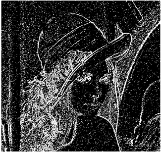
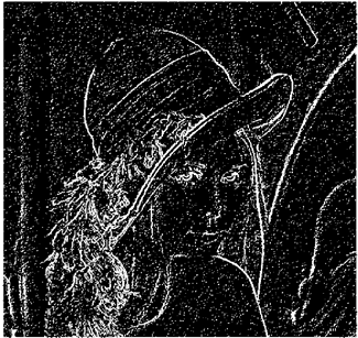
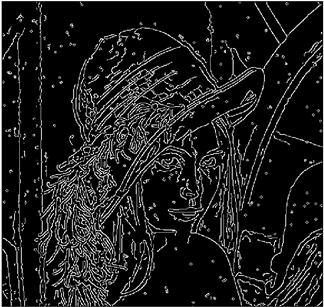
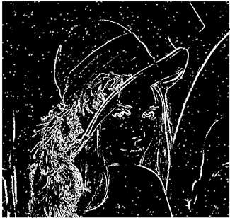
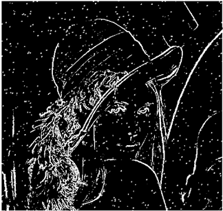
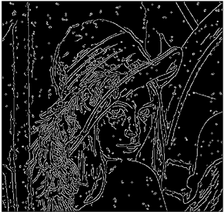
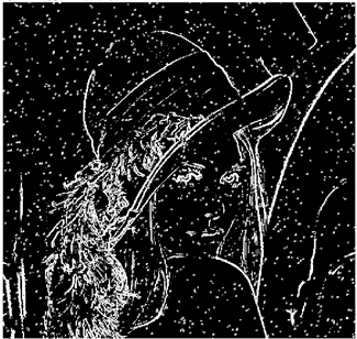
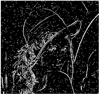
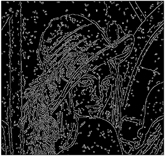
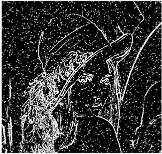
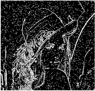
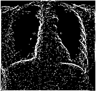
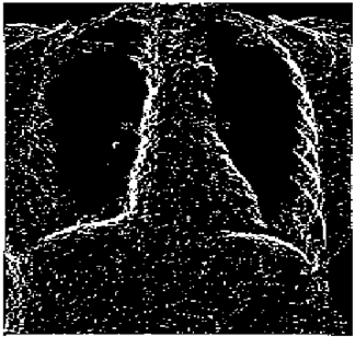
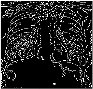
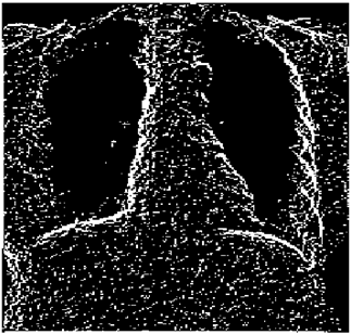
As shown in Table 6, the PFOM values related to the smooth composition are higher than those of the standard composition in all cases. Table 7, Table 8, Table 9, Table 10, Table 11, Table 12, Table 13 and Table 14 also provide a visual demonstration supporting this conclusion. As is quite obvious from these tables, the density of noise in the edge-detected images of smooth composition is always less than that of the standard composition. Furthermore, the Canny edge detector is also highly prone to noises and is unable to decrease the noise density.

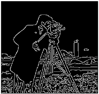
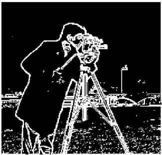
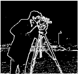
Table 7. Edge-detected image of “Cameraman” after binarization for different noises.

Noise	Canny	Standard	Smooth
No noise
G(0.001)
G(0.002)
G(0.003)
I(0.25%)
I(0.5%)
I(1%)

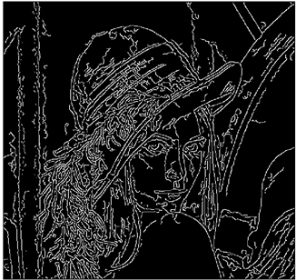
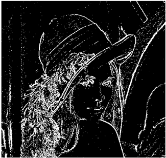
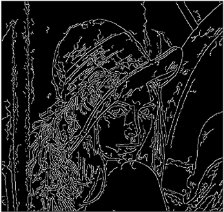
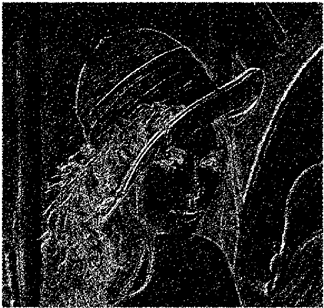
Table 8. Edge-detected image of “Lena” after binarization for different noises.

Noise	Canny	Standard	Smooth
No noise
G(0.001)
G(0.002)
G(0.003)
I(0.25%)
I(0.5%)
I(1%)

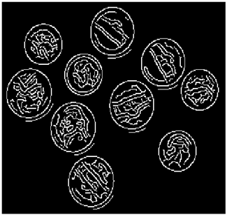
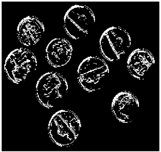
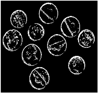
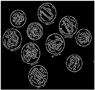
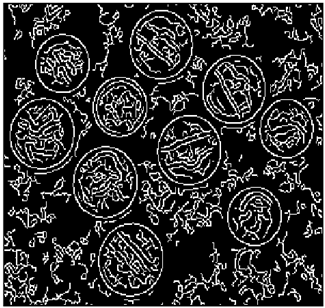
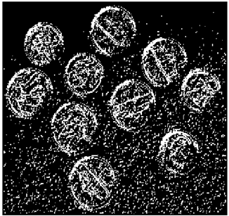
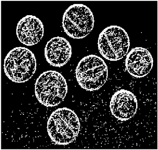
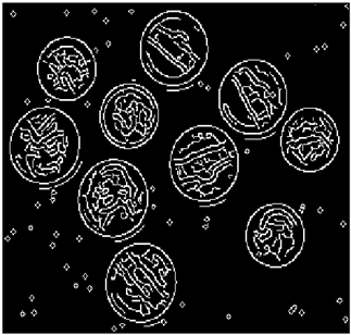
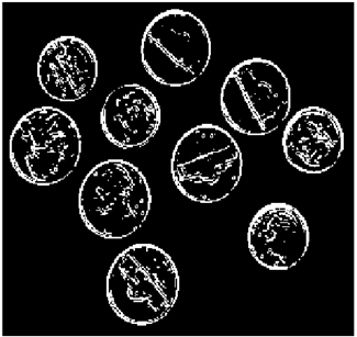
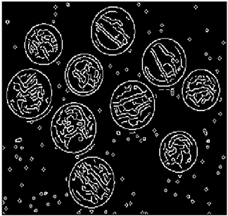
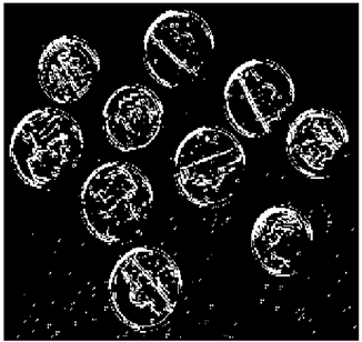
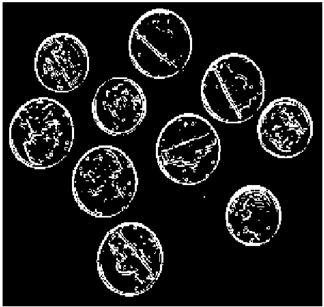
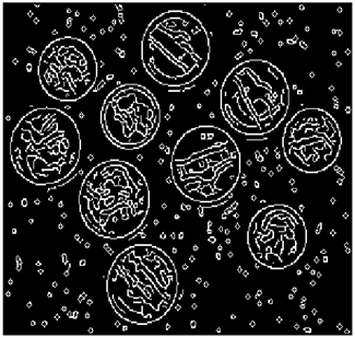
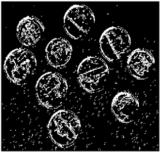
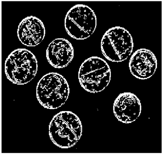
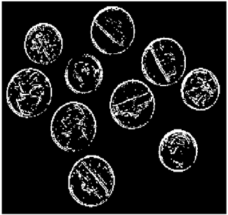
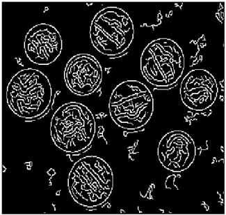
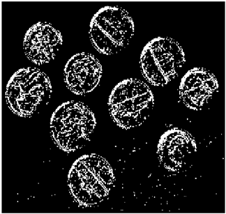
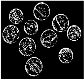
Table 9. Edge-detected image of “Coins” after binarization for different noises.

Noise	Canny	Standard	Smooth
No noise
G(0.001)
G(0.002)
G(0.003)
I(0.25%)
I(0.5%)
I(1%)

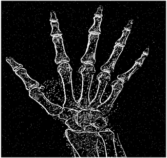
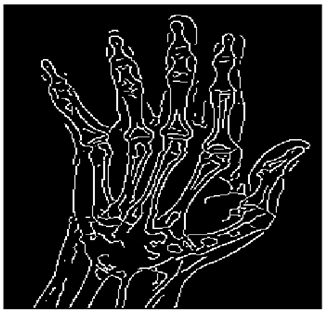
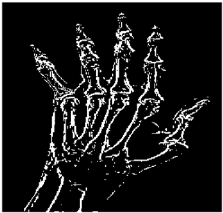
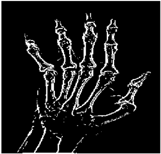
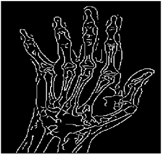
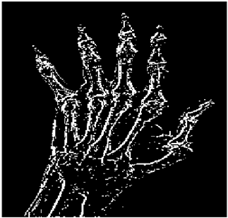
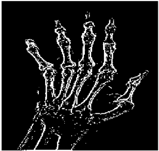
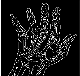
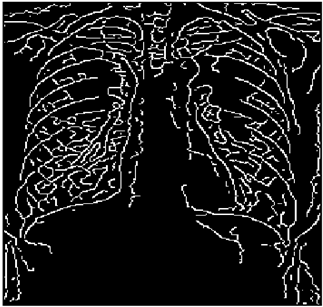
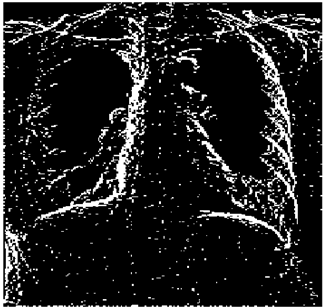
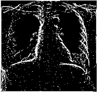
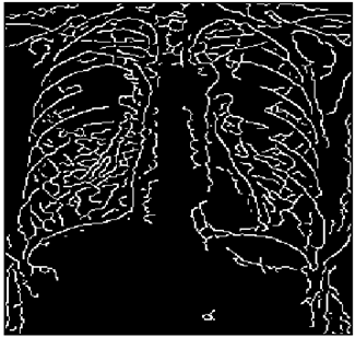
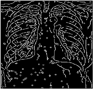
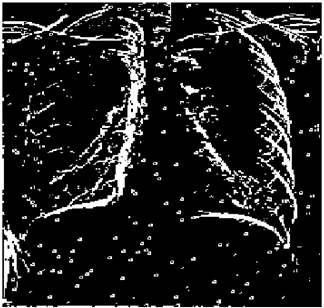
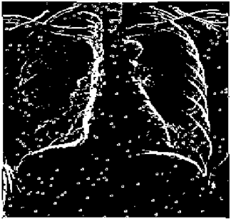
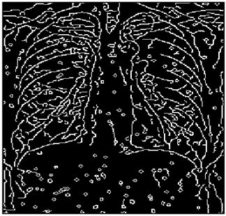
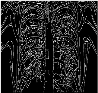
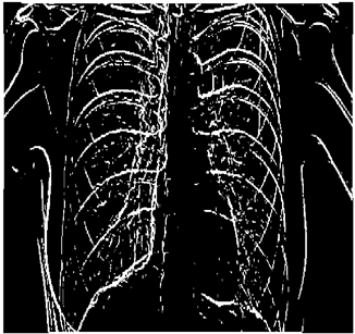
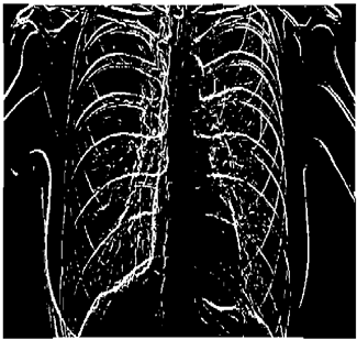
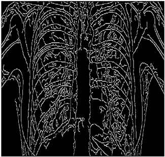
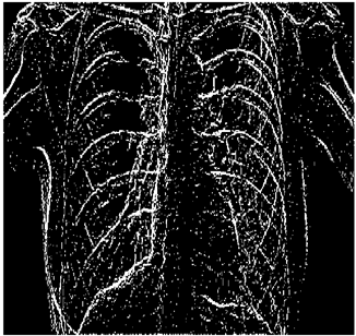
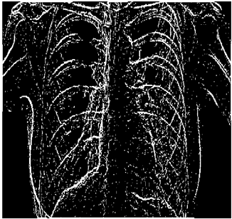
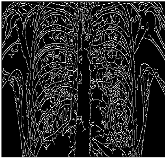
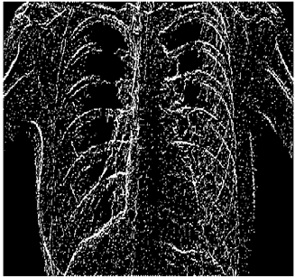
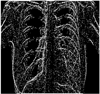
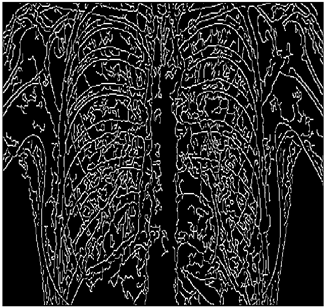
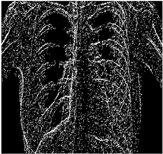
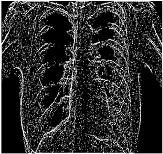
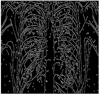
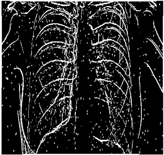
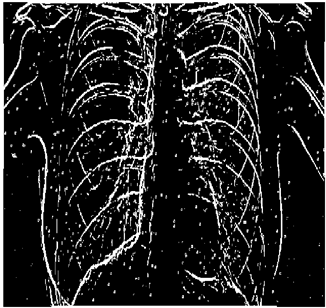
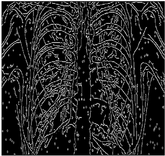
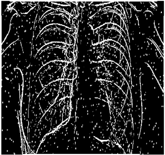
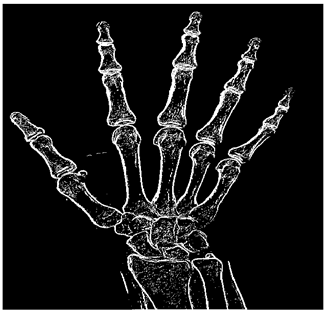
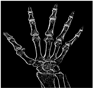
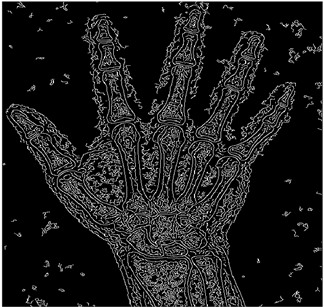
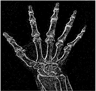
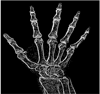
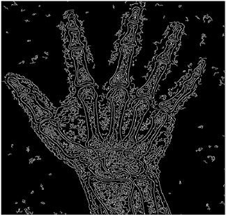
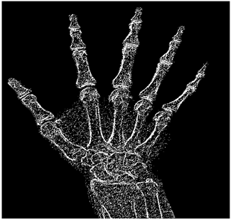
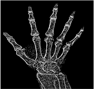
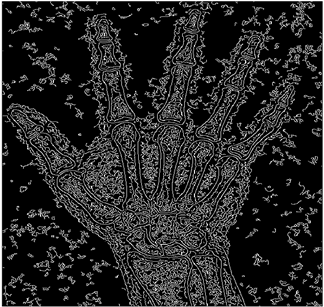
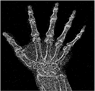
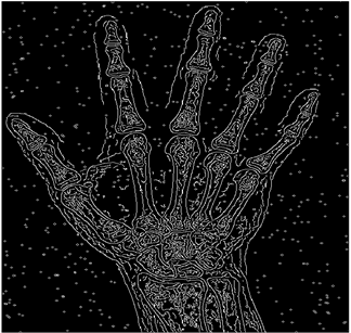
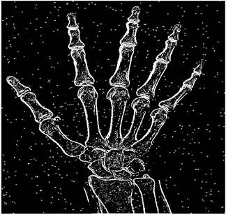
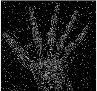
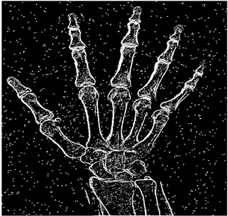
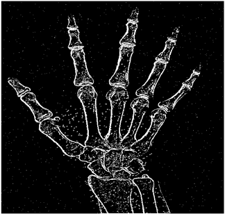
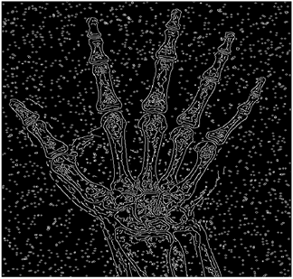
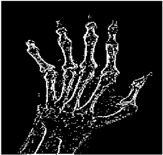
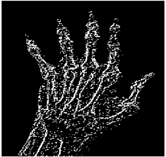
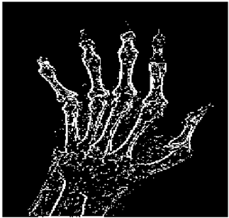
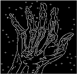
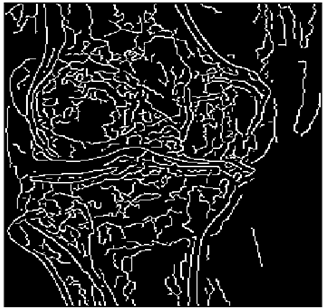
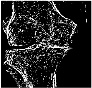
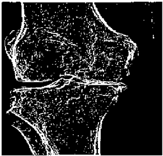
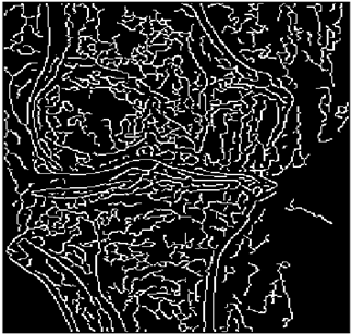
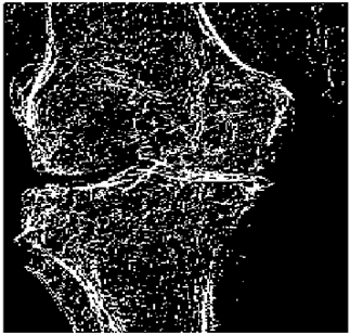
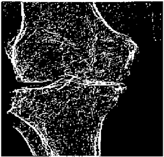
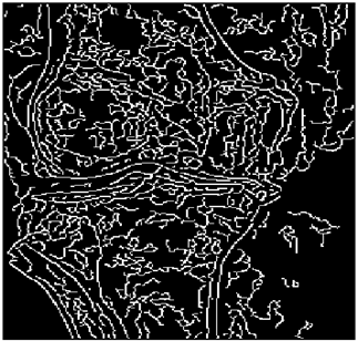
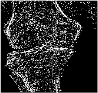
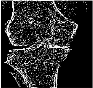
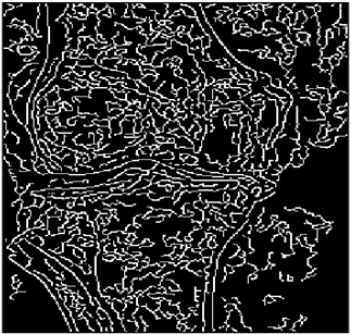
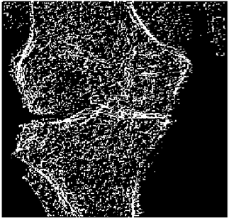
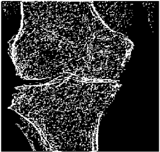
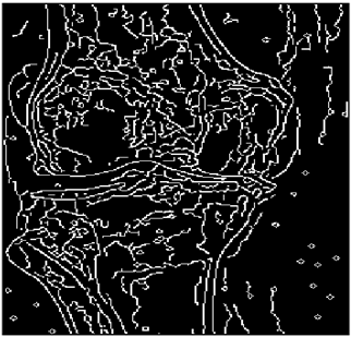
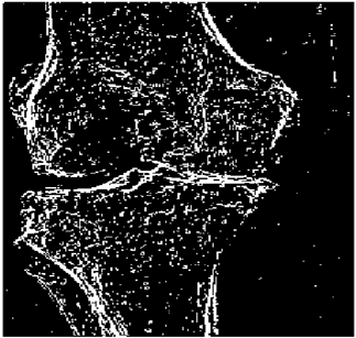
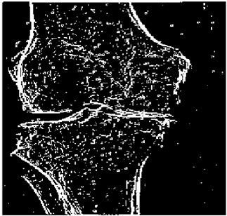
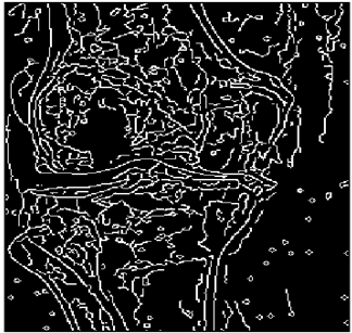
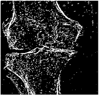
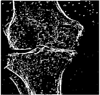
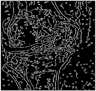
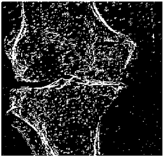
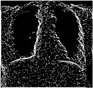
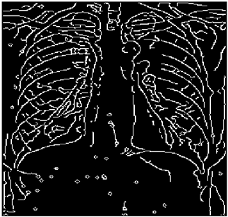
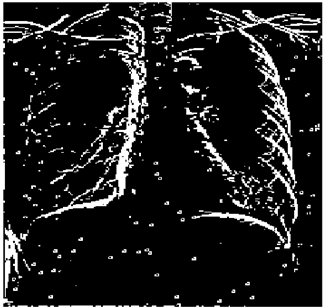
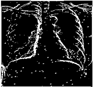
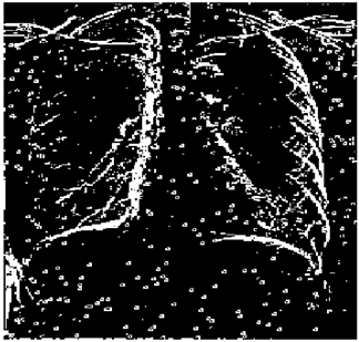
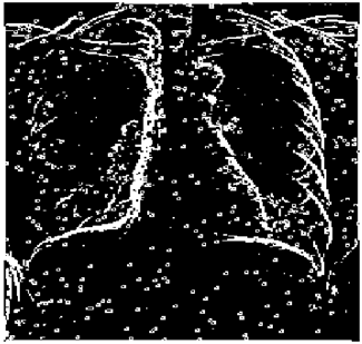
Table 10. Edge-detected image of “X-ray 1” after binarization for different noises.

Noise	Canny	Standard	Smooth
No noise
G(0.001)
G(0.002)
G(0.003)
I(0.25%)
I(0.5%)
I(1%)

Table 11. Edge-detected image of “X-ray 2” after binarization for different noises.

Noise	Canny	Standard	Smooth
No noise
G(0.001)
G(0.002)
G(0.003)
I(0.25%)
I(0.5%)
I(1%)

Table 12. Edge-detected image of “X-ray 3” after binarization for different noises.

Noise	Canny	Standard	Smooth
No noise
G(0.001)
G(0.002)
G(0.003)
I(0.25%)
I(0.5%)
I(1%)

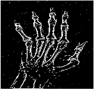
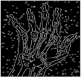
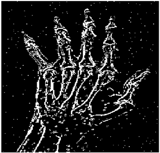
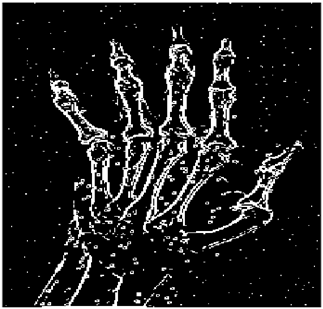
Table 13. Edge-detected image of “X-ray 4” after binarization for different noises.

Noise	Canny	Standard	Smooth
No noise
G(0.001)
G(0.002)
G(0.003)
I(0.25%)
I(0.5%)
I(1%)

Table 14. Edge-detected image of “X-ray 5” after binarization for different noises.

Noise	Canny	Standard	Smooth
No noise
G(0.001)
G(0.002)
G(0.003)
I(0.25%)
I(0.5%)
I(1%)

Experimental Results

This subsection of the manuscript dives deeper into the details of the visual tables, i.e., Table 7, Table 8, Table 9, Table 10, Table 11, Table 12, Table 13 and Table 14.

Table 7 shows that:

• In all cases, the Canny edge detector detects more edge pixels than both fuzzy compositions.
• As the level of noise increases, all three methods become adversely affected by the noise, and still more edges are detected by Canny.
• However, in all cases, the PFOM value for the smooth composition is always greater than the PFOM value for the standard composition, according to Table 6.

Table 8 shows that:

• In all cases, the Canny edge detector detects more edge pixels than both fuzzy compositions.
• As the level of noise increases, Canny and standard composition become adversely affected by the noise, and still more edges are detected by Canny; however, most of the detected edges by Canny are misdetections due to the impact of noise. As is obvious from this table, the smooth composition provides a better image with reduced noise density.
• In all cases, the PFOM value for the smooth composition is always greater than the PFOM value for the standard composition, according to Table 6.

Table 9 shows the following:

• In all cases, the Canny edge detector detects more edge pixels than both fuzzy compositions.
• As the level of noise increases, Canny and standard composition become adversely affected by noise, and still more edges are detected by Canny; however, most of the detected edges by Canny are misdetections due to the impact of noise. As is obvious from this table, the standard and smooth compositions provide a better image with reduced noise density.
• However, in all cases, the PFOM value for the smooth composition is always greater than the PFOM value for the standard composition, according to Table 6.

Table 10 shows the following:

• In all cases, the Canny edge detector detects more edge pixels than both fuzzy compositions.
• As the level of noise increases, Canny and standard composition become adversely affected by the noise, and still more edges are detected by Canny; however, most of the detected edges by Canny are misdetections due to the impact of noise. As is obvious from this table, the smooth composition provides a better image with reduced noise density.
• In all cases, the PFOM value for the smooth composition is always greater than the PFOM value for the standard composition, according to Table 6.

For Table 11, Table 12 and Table 13, the same points of Table 10 can be made. Therefore, for the sake of brevity, the points are not mentioned.

Table 14 shows the following:

• In all cases, the Canny edge detector detects more edge pixels than both fuzzy compositions.
• As the level of noise increases, all three methods become adversely affected by the noise, and still more edges are detected by Canny; however, most of the detected edges by Canny are misdetections due to the impact of noise. As is obvious from this table, the standard composition as well as the smooth composition somehow show equal performance in reducing noise density.
• However, in all cases, the PFOM value for the smooth composition is always greater than the PFOM value for the standard composition, according to Table 6.

6. Conclusions

The contribution of the present manuscript is twofold. Firstly, it studies the bounded variation of the smooth fuzzy models and quantifies the results for the application of different fuzzy compositions for noise removal. On the other hand, it applies the smooth fuzzy compositions for the edge detection of digital images. The results have been expressed in terms of the widely used Pratt’s Figure of Merit (PFOM) as well as the visual observations of the images in the presence of the different levels of noise. The presented experiments could show the superiority of the smooth fuzzy filters over the standard fuzzy filters through numerical comparisons of the error in performance and visual observation. In the theoretical studies, the involved MF has not been supposed to have a special shape, and therefore, we leave the designer free to select it based on the desire for the improvement of the fuzzy edge detection algorithm by the involvement of the smooth compositions.

7. Future Works

Fuzzy edge detection methods are being widely used in the processing of medical images. Hence, future work can be dedicated to the application of the proposed technique in a wide range of investigations on the extension of the earlier works on the detection of diabetic retinopathy [49], in the maculopathy of eye fundus images [50], or for brain tumor detection and treatments [51,52,53]. In addition, other types of smooth compositions can be used in the wider domain of datasets for comparison with the standard fuzzy compositions for noise removal and edge recovery.

References

- Gonzalez, C.I.; Melin, P.; Castro, J.R.; Castillo, O.; Mendoza, O. Optimization of interval type-2 fuzzy systems for image edge detection. Appl. Soft Comput. 2016, 47, 631–643. [Google Scholar] [CrossRef]
- Verma, O.P.; Parihar, A.S. An Optimal Fuzzy System for Edge Detection in Color Images Using Bacterial Foraging Algorithm. IEEE Trans. Fuzzy Syst. 2017, 25, 114–127. [Google Scholar] [CrossRef]
- Li, O.; Shui, P.L. Noise-robust color edge detection using anisotropic morphological directional derivative matrix. Signal Process. 2019, 165, 90–103. [Google Scholar] [CrossRef]
- Haq, I.; Anwar, S.; Shah, K.; Khan, M.T.; Shah, S.A. Fuzzy Logic Based Edge Detection in Smooth and Noisy Clinical Images. PLoS ONE 2015, 10, e0138712. [Google Scholar] [CrossRef] [PubMed]
- Melin, P.; Gonzalez, C.I.; Castro, J.R.; Mendoza, O.; Castillo, O. Edge-Detection Method for Image Processing Based on Generalized Type-2 Fuzzy Logic. IEEE Trans. Fuzzy Syst. 2014, 22, 1515–1525. [Google Scholar] [CrossRef]
- Uguz, S.; Sahin, U.; Sahin, F. Edge detection with fuzzy cellular automata transition function optimized by PSO. Comput. Electr. Eng. 2015, 43, 180–192. [Google Scholar] [CrossRef]
- Veganzones, M.A.; Tochon, G.; Dalla-Mura, M.; Plaza, A.J.; Chanussot, J. Hyperspectral Image Segmentation Using a New Spectral Unmixing-Based Binary Partition Tree Representation. IEEE Trans. Image Process. 2014, 23, 3574–3589. [Google Scholar] [CrossRef]
- Ziółko, B.; Emms, D.; Ziółko, M. Fuzzy Evaluations of Image Segmentation. IEEE Trans. Fuzzy Syst. 2018, 26, 1789–1799. [Google Scholar] [CrossRef]
- Tang, Y.; Ren, F.; Pedrycz, W. Fuzzy C-Means clustering through SSIM and patch for image segmentation. Appl. Soft Comput. 2020, 87, 105928. [Google Scholar] [CrossRef]
- Singh, V.; Dev, R.; Dhar, N.K.; Agrawal, P.; Verma, N.K. Adaptive Type-2 Fuzzy Approach for Filtering Salt and Pepper Noise in Grayscale Images. IEEE Trans. Fuzzy Syst. 2018, 26, 3170–3176. [Google Scholar] [CrossRef]
- Mosleh, A.; Bouguila, N.; Hamza, A.B. Image Text Detection Using a Bandlet-Based Edge Detector and Stroke Width Transform. In Proceedings of the British Machine Vision Conference 2012, Surrey, UK, 3–7 September 2012; Bowden, R., Collomosse, J., Mikolajczyk, K., Eds.; BMVA: Durham, UK, 2012; pp. 63.1–63.12. [Google Scholar] [CrossRef] [Green Version]
- Azeroual, A.; Afdel, K. Fast Image Edge Detection based on Faber Schauder Wavelet and Otsu Threshold. Heliyon 2017, 3, e00485. [Google Scholar] [CrossRef] [PubMed] [Green Version]
- uddin Khan, N.; Arya, K.V. A new fuzzy rule based pixel organization scheme for optimal edge detection and impulse noise removal. Multimed. Tools Appl. 2020, 79, 33811–33837. [Google Scholar] [CrossRef]
- Molina, J.M.; Martín, M.J.; Isasi, P.; Sanchis, A. A fuzzy reasoning system for boundary detection in radiological images. In Proceedings of the 1998 IEEE International Conference on Fuzzy Systems Proceedings. IEEE World Congress on Computational Intelligence (Cat. No.98CH36228), Anchorage, AK, USA, 4–9 May 1998; Volume 2, pp. 1524–1529. [Google Scholar] [CrossRef] [Green Version]
- Abdullah Yahya, A.A.; Tan, J.; Su, B.; Liu, K.; Hadi, A.N. Image edge detection method based on anisotropic diffusion and total variation models. J. Eng. 2019, 2019, 455–460. [Google Scholar] [CrossRef]
- Soria, R.; Sanchis, A.; Molina, J.M. Fuzzy colour distance applied to region growing in image processing. In Proceedings of the EUSFLAT-ESTYLF Joint Conference, Palma de Mallorca, Spain, 22–25 September 1999; Mayor, G., Suñer, J., Eds.; Universitat de les Illes Balears: Palma de Mallorca, Spain, 1999; pp. 259–262. [Google Scholar]
- Rudin, L.I.; Osher, S.; Fatemi, E. Nonlinear total variation based noise removal algorithms. Phys. D Nonlinear Phenom. 1992, 60, 259–268. [Google Scholar] [CrossRef]
- Sadjadi, E.N.; Garcia Herrero, J.; Manuel Molina, J.; Hatami Moghaddam, Z. On Approximation Properties of Smooth Fuzzy Models. Int. J. Fuzzy Syst. 2018, 20, 2657–2667. [Google Scholar] [CrossRef]
- Sadjadi, E.N.; Menhaj, M.B.; Herrero, J.G.; Molina Lopez, J.M. How Effective are Smooth Compositions in Predictive Control of TS Fuzzy Models? Int. J. Fuzzy Syst. 2019, 21, 1669–1686. [Google Scholar] [CrossRef]
- Sadjadi, E.N.; Garcia, J.; Molina Lopez, J.M.; Borzabadi, A.H.; Abchouyeh, M.A. Fuzzy Model Identification and Self Learning with Smooth Compositions. Int. J. Fuzzy Syst. 2019, 21, 2679–2693. [Google Scholar] [CrossRef]
- Sadjadi, E.N.; Ebrahimi, M.; Gachloo, Z. Discussion on Accuracy of Approximation with Smooth Fuzzy Models. In Proceedings of the 2020 IEEE Canadian Conference on Electrical and Computer Engineering (CCECE), London, ON, Canada, 30 August–2 September 2020; pp. 1–6. [Google Scholar] [CrossRef]
- Sadjadi, E.N. On the Monotonicity of Smooth Fuzzy Systems. IEEE Trans. Fuzzy Syst. 2021, 29, 3947–3952. [Google Scholar] [CrossRef]
- Sadjadi, E.N. Smooth compositions are candidates for robust fuzzy systems. Fuzzy Sets Syst. 2022, 426, 66–93. [Google Scholar] [CrossRef]
- Sadjadi, E.N.; Menhaj, M.B.; Sadrian Zadeh, D.; Moshiri, B. Stability Analysis of Smooth Positive Fuzzy Systems. In Proceedings of the 2020 IEEE Canadian Conference on Electrical and Computer Engineering (CCECE), London, ON, Canada, 30 August–2 September 2020; pp. 1–6. [Google Scholar] [CrossRef]
- Sadjadi, E.N.; Menhaj, M.B.; Sadrian Zadeh, D.; Moshiri, B. Fuzzy Adaptive Control of a Knee-Joint Orthosis for the Smooth Tracking. In Proceedings of the 2020 IEEE Canadian Conference on Electrical and Computer Engineering (CCECE), London, ON, Canada, 30 August–2 September 2020; pp. 1–6. [Google Scholar] [CrossRef]
- Sadjadi, E.N. Smooth Compositions Made Stabilization of Fuzzy Systems: Easy and More Robust. IEEE Trans. Cybern. 2021, 52, 5819–5827. [Google Scholar] [CrossRef]
- Sadjadi, E.N. Direct Approximation of Error in Fuzzy Modeling Using a Simple Formulation. IEEE Trans. Fuzzy Syst. Appear. 2022; submitted. [Google Scholar]
- Sadrian Zadeh, D.; Sadjadi, E.N.; Moshiri, B. Training Error Approximation Through the State-Space Representation of the Fuzzy Model. In Proceedings of the 2021 American Control Conference (ACC), New Orleans, LA, USA, 25–28 May 2021; pp. 4357–4362. [Google Scholar] [CrossRef]
- Sadjadi, E.N. Sensitivity Analysis of Smooth Fuzzy Models. Frankl. Inst. Appear. 2022; submitted. [Google Scholar]
- Sadjadi, E.N. Smooth Compositions Enhance the Stability of Fuzzy Systems Due to Shrinking Behavior of the Structure. Fuzzy Sets Syst. Appear. 2022; submitted. [Google Scholar]
- Sadjadi, E.N. Smooth Fuzzy Models Higher the Accuracy and Reduce the Parameters Dimension: A Proof of Concept in the Frequency Domain. Fuzzy Sets Syst. Appear. 2022; submitted. [Google Scholar]
- Sadjadi, E.N. On the connection of smooth fuzzy models with the kernel machines. Int. J. Fuzzy Syst. Appear. 2022; submitted. [Google Scholar]
- Giusti, E. Minimal Surfaces and Functions of Bounded Variation, 1st ed.; Birkhäuser: Boston, MA, USA, 1984; p. XII, 240. [Google Scholar] [CrossRef]
- Moreau, J.J.; Panagiotopoulos, P.D.; Strang, G. (Eds.) Topics in Nonsmooth Mechanics, 1st ed.; Birkhäuser: Boston, MA, USA, 1988; p. XIII, 329. [Google Scholar]
- Strong, D.; Chan, T. Edge-preserving and scale-dependent properties of total variation regularization. Inverse Probl. 2003, 19, S165–S187. [Google Scholar] [CrossRef]
- Chambolle, A. An Algorithm for Total Variation Minimization and Applications. J. Math. Imaging Vis. 2004, 20, 89–97. [Google Scholar] [CrossRef]
- Leoni, G. A First Course in Sobolev Spaces, 2nd ed.; Graduate Studies in Mathematics; American Mathematical Society: Providence, RI, USA, 2009; p. 607. [Google Scholar]
- Getreuer, P. Rudin-Osher-Fatemi Total Variation Denoising using Split Bregman. Image Process. Line 2012, 2, 74–95. [Google Scholar] [CrossRef]
- Abdou, I.E.; Pratt, W.K. Quantitative design and evaluation of enhancement/thresholding edge detectors. Proc. IEEE 1979, 67, 753–763. [Google Scholar] [CrossRef]
- Pratt, W.K. Digital Image Processing, 2nd ed.; John Wiley & Sons: Hoboken, NJ, USA, 1991; p. 720. [Google Scholar]
- Umbaugh, S.E. Computer Imaging: Digital Image Analysis and Processing; CRC Press: Boca Raton, FL, USA, 2005. [Google Scholar]
- Pande, S.; Singh Bhadouria, V.; Ghoshal, D. A study on edge marking scheme of various standard edge detectors. Int. J. Comput. Appl. 2012, 44, 33–37. [Google Scholar] [CrossRef]
- Kumar, M.; Saxena, R. Algorithm and Technique on Various Edge Detection: A Survey. Signal Image Process. Int. J. (SIPIJ) 2013, 4, 65–75. [Google Scholar] [CrossRef]
- Sadiq, B.O.; Sani, S.M.; Garba, S. Edge Detection: A Collection of Pixel based Approach for Colored Images. Int. J. Comput. Appl. 2015, 113, 29–32. [Google Scholar] [CrossRef] [Green Version]
- Haddad, A. Stability in a class of variational methods. Appl. Comput. Harmon. Anal. 2007, 23, 57–73, Special Issue on Mathematical Imaging. [Google Scholar] [CrossRef] [Green Version]
- Chan, T.F.; Esedoglu, S. Aspects of Total Variation Regularized L1 Function Approximation. SIAM J. Appl. Math. 2005, 65, 1817–1837. [Google Scholar] [CrossRef] [Green Version]
- Dong, Y.; Zeng, T. A Convex Variational Model for Restoring Blurred Images with Multiplicative Noise. SIAM J. Imaging Sci. 2013, 6, 1598–1625. [Google Scholar] [CrossRef] [Green Version]
- Le, T.; Chartrand, R.; Asaki, T.J. A Variational Approach to Reconstructing Images Corrupted by Poisson Noise. J. Math. Imaging Vis. 2007, 27, 257–263. [Google Scholar] [CrossRef]
- Kumar, S.; Adarsh, A.; Kumar, B.; Singh, A.K. An automated early diabetic retinopathy detection through improved blood vessel and optic disc segmentation. Opt. Laser Technol. 2020, 121, 105815. [Google Scholar] [CrossRef]
- Rahim, S.S.; Palade, V.; Jayne, C.; Holzinger, A.; Shuttleworth, J. Detection of Diabetic Retinopathy and Maculopathy in Eye Fundus Images Using Fuzzy Image Processing. In Proceedings of the Brain Informatics and Health, 8th International Conference, BIH 2015, London, UK, 30 August–2 September 2015; Guo, Y., Friston, K., Aldo, F., Hill, S., Peng, H., Eds.; Springer: Berlin/Heidelberg, Germany, 2015; Volume 9250, pp. 379–388. [Google Scholar] [CrossRef]
- Pereira, S.; Pinto, A.; Alves, V.; Silva, C.A. Brain Tumor Segmentation Using Convolutional Neural Networks in MRI Images. IEEE Trans. Med. Imaging 2016, 35, 1240–1251. [Google Scholar] [CrossRef]
- Mohan, G.; Subashini, M.M. MRI based medical image analysis: Survey on brain tumor grade classification. Biomed. Signal Process. Control. 2018, 39, 139–161. [Google Scholar] [CrossRef]
- Chatterjee, S.; Das, A. A novel systematic approach to diagnose brain tumor using integrated type-II fuzzy logic and ANFIS (adaptive neuro-fuzzy inference system) model. Soft Comput. 2019, 24, 11731–11754. [Google Scholar] [CrossRef]
Publisher’s Note: MDPI stays neutral with regard to jurisdictional claims in published maps and institutional affiliations. |
© 2022 by the authors. Licensee MDPI, Basel, Switzerland. This article is an open access article distributed under the terms and conditions of the Creative Commons Attribution (CC BY) license (https://creativecommons.org/licenses/by/4.0/).