Quantile-Wavelet Nonparametric Estimates for Time-Varying Coefficient Models

Abstract

The paper considers quantile-wavelet estimation for time-varying coefficients by embedding a wavelet kernel into quantile regression. Our methodology is quite general in the sense that we do not require the unknown time-varying coefficients to be smooth curves of a common degree or the errors to be independently distributed. Quantile-wavelet estimation is robust to outliers or heavy-tailed data. The model is a dynamic time-varying model of nonlinear time series. A strong Bahadur order $O\left\{{\left(\frac{2^m}{n}\right)}^{3/4}{(logn)}^{1/2}\right\}$ for the estimation is obtained under mild conditions. As applications, the rate of uniform strong convergence and the asymptotic normality are derived.

1. Introduction

The trending time-varying time series models have gained a lot of attention during the last three decades because they are increasingly used to observe changes in their dynamic structure, which have been applied to economics and finance [1,2]. When the time span of interest covers different economic periods, the parameters of the corresponding statistical models should be allowed to change with time; see references [3,4,5,6,7], among others. Varying coefficient models are flexible models for describing the dynamic structure of data, which have been extensively studied based on mean regression, for example, references [8,9,10,11,12], among others and the references therein. However, the important features of the joint distribution of the response and the covariates can not be well captured by mean regression.

In this paper, we consider the time-varying coefficient quantile regression models: the conditional $\tau$th quantile of $Y_i$ given ${\mathit{X}}_i$ and a prespecified quantile $\tau$,

$$Q_{\tau }\left(Y_i\right|{\mathit{X}}_i)=inf\left\{s:F_{Y_i|{\mathit{X}}_i}\left(s\right|{\mathit{X}}_i)>\tau \right\}={\mathit{X}}_i^T{\mathit{\beta }}_{\tau }\left(t_i\right),i=1,\cdots ,n,$$

(1)

where $t_i=i/n$, $Y_i$ are responses, ${\mathit{\beta }}_{\tau }(·)={({\beta }_{1,\tau }(·),\cdots ,{\beta }_{p,\tau }(·))}^T$ is a p-dimensional vector of unspecified functions defined on $[0,1]$, ${\mathit{X}}_i={(X_{i1},\cdots ,X_{ip})}^T$ are p-dimensional explanatory variables. We can write Equation (1) in the form

$$Y_i={\mathit{X}}_i^T{\mathit{\beta }}_{\tau }\left(t_i\right)+{ϵ}_{\tau ,i},i=1,\cdots ,n,$$

(2)

where the errors ${ϵ}_{\tau ,i}$ satisfy $Q_{\tau }\left({ϵ}_{\tau ,i}\right|{\mathit{X}}_i)=0$ almost surely. Quantile regression has also been emerged as an essential statistical tool in many scientific fields; see [13]. To simplify notations, we omit the subscript $\tau$ from the function ${\mathit{\beta }}_{\tau }(·)$ and ${ϵ}_{\tau ,i}$ subsequently.

To estimate the varying coefficients in quantile regression models in Equation (2), references [7,14,15] used the kernel method, and references [16,17] considered regression splines. To our knowledge, wavelet has not been considered in quantile regression with varying coefficients. Wavelet techniques can detect and represent localized features and can also create localized features on synthesis while being efficient in terms of computational speed and storage. It has received much attention from mathematicians, engineers and statisticians. Wavelet has been introduced for nonparametric regression, for example, references [18,19,20,21,22], and so on. For wavelet smoothing applied to nonparametric models, reference [18] is a key reference that introduces wavelet versions of some classical kernel and orthogonal series estimators and studies their asymptotic properties. Reference [23] provided asymptotic bias and variance of a wavelet estimator for a regression function under a stochastic mixing process. Reference [24] considered a wavelet estimator for the mean regression function with strong mixing errors and investigated their asymptotic rates of convergence by using the thresholding of the empirical wavelet coefficients. References [25,26] showed Berry–Esseen-type bounds on wavelet estimators for semiparametric models under dependent errors. For varying coefficient models, references [27,28] provided wavelet estimation and studied convergence rate and asymptotic normality under i.i.d. errors, and reference [29] discussed these asymptotics of the wavelet estimators based on censored dependent data. However, all of the above wavelet estimators are based on mean regression by the least-squares method.

In the paper, we propose a quantile-wavelet method for time-varying coefficient models in Equation (2) with an $\alpha$-mixing errors stochastic process. The proposed methodology is quite general in the sense that we do not require coefficient $\mathit{\beta }(·)$ to be smooth curves of a common degree, it does not suffer from the curse of dimensionality, it is robust to outlier or heavy-tailed data, and it is a dynamic model for nonlinear time series. Bahadur representation, rate of convergence and asymptotic normality of quantile-wavelet estimators will be established. Bahadur representation theory seeks to approximate a statistical estimate by a sum of variables with a higher-order remained. It has been a major statistical theory issue since Bahadur’s pioneering work on quantiles [30]; see [31], among others. Recently, reference [32] investigated the Bahadur representation for sample quantiles under $\phi$-mixing sequence; reference [33] gave an M-estimation for time-varying coefficient models with $\alpha$-mixing errors and established Bahadur representation in probability. In the paper, we will establish Bahadur representation with probability 1 (almost surely) for quantile-wavelet estimates in the models Equations (1) and (2).

Throughout, we assume that $\{{\mathit{X}}_i,{ϵ}_i\}$ is a stationary $\alpha$-mixing sequence. Recall that a sequence $\{{\zeta }_k,k\ge 1\}$ is said to be $\alpha$-mixing (or strong mixing) if the mixing coefficients

$$\alpha \left(m\right)=sup\left\{\right|P(A\cap B)-P\left(A\right)P\left(B\right)|:A\in {\mathcal{F}}_{-\infty }^k,B\in {\mathcal{F}}_{k+m}^{\infty }\}$$

converge to zero as $m\to \infty$, where ${\mathcal{F}}_l^k$ denotes the $\sigma$-field generated by $\{{\zeta }_i,l\le i\le k\}$. We refer to the monograph of [34,35] for some properties or more mixing conditions.

The rest of this article is organized as follows. In Section 2, we present wavelet kernel and quantile-wavelet estimation for the model (2). Bahadur representation of quantile-wavelet estimators and their applications are given in Section 3. Technical proofs are provided in Section 4. Some simulation studies are conducted in Section 5.

2. Quantile-Wavelet Estimation

In the paper, the time-varying coefficient function is retrieved by a wavelet-based reproducing kernel Hilbert space (RKHS). An RKHS is a Hilbert space in which all the point evaluations are bounded linear functions. Let $f\in \mathcal{H}$ be a Hilbert space of functions on some domain $\mathcal{I}$. For $t\in \mathcal{I}$, then there exists an element $k_t\in \mathcal{H}$, such that

$$f\left(t\right)=⟨k_t,f⟩,\forall f\in \mathcal{H},$$

where $⟨·,·⟩$ is the inner product in $\mathcal{H}$. Set $⟨k_t,k_s⟩=K(t,s)$, which is called the reproducing kernel. Let $k_t=K(t,·)$, and then $⟨K(t,·),K(s,·)⟩=K(t,s)$.

A multiresolution analysis is a sequence of closed subspaces $\{V_m,m\in \mathbb{Z}\}$ in ${\mathcal{L}}_2\left(\mathbb{R}\right)$ such that they lie in a containment hierarchy,

$$\cdots \subset V_{-2}\subset V_{-1}\subset V_0\subset V_1\subset V_2\subset \cdots ,$$

(3)

where ${\mathcal{L}}_2\left(\mathbb{R}\right)$ is the collection of square-integrable functions over the real line. The hierarchy Equation (3) is constructed such that (i) V-spaces are self-similar, $f\left(2^{m}x\right)\in V_m\mathrm{iff}$$f\left(x\right)\in V_0$, and (ii) there exists a scaling function $\varphi \in V_0$ whose integer-translate $V_0=\{f\in {\mathcal{L}}_2\left(\mathbb{R}\right)|f\left(x\right)={\sum }_{k\in \mathbb{Z}}{c}_k\varphi (x-k)\}$, and for which the set $\left\{\varphi \right(·-k),k\in \mathbb{Z}\}$ is an orthonormal basis. Wavelet analysis requires a description of two related and suitably chosen orthonormal basic functions: the scaling function $\varphi$ and the wavelet $\psi$. A wavelet system is generated by dilation and translation of $\varphi$ and $\psi$ through

$${\varphi }_{m,k}\left(t\right)=2^{m/2}\varphi (2^{m}t-k),{\psi }_{m,k}\left(t\right)=2^{m/2}\psi (2^{m}t-k),m,k\in \mathbb{Z}.$$

Therefore, $\{{\varphi }_{0k},k\in \mathbb{Z}\}$ and $\{{\varphi }_{mk},k\in \mathbb{Z}\}$ are the orthogonal bases of $V_0$ and $V_m$, respectively. From Moore-Aronszajn’s theorem [36], it follows that

$$K(t,s)=\sum _k\varphi (t-k)\varphi (s-k)$$

is a reproducing kernel of $V_0$. By self-similarity of multiresolution subspaces,

$$K_m(t,s)=2^{m}K(2^{m}t,2^{m}s)$$

is a reproducing kernel of $V_m$, and then the projection of g on the space $V_m$ is given by

$${\mathbb{P}}_{V_m}g\left(t\right)=\int K_m(t,s)g\left(s\right)ds.$$

It motivates us to define a quantile-wavelet estimator of $\mathit{\beta }\left(t\right)$ by

$$\widehat{\mathit{\beta }}\left(t\right)={\mathrm{argmin}}_{\mathit{b}}\sum _{i=1}^n{\rho }_{\tau }\left\{y_i-{\mathit{X}}_i^T\mathit{b}\right\}{\int }_{A_i}{K}_m(t,s)ds,$$

(4)

where ${\rho }_{\tau }\left(u\right)=u(\tau -I\{u<0\})$ with $u\in \mathbb{R}$ called the loss (“check”) function, $I_B$ is the indicator function of any set B, and $A_i$ are intervals that partition [0, 1], so that $t_i\in A_i$. One way of defining the intervals $A_i=[s_{i-1},s_i)$ is by taking $s_0=0$, $s_n=1$, and $s_i=(t_i+t_{i+1})/2$, $i=1,\cdots ,n-1$.

Note that many other nonparametric methods can be used here, including spline and Kernel approaches. However, they might not be rich enough to characterize the local properties of the time-varying coefficient function. In the following section, we will present the asymptotic properties of the quantile-wavelet estimator Equation (4).

3. Bahadur Representation and Its Applications

Let ${\mathcal{H}}^{\nu }$ be the collection of all functions on $[0, 1]$ with order $\nu >0$ in Sobolev space, which is a very general space. The degree of smoothness of the true coefficient functions determines how well the functions can be approximated. Functions belonging to ${\mathcal{H}}^{\nu }$ for $1/2<\nu <3/2$ are not continuously differentiable. It is worth stressing that the wavelet approach allows us to obtain rates under much weaker assumptions than second-order differentiability. Denote $\mathit{X}=({\mathit{X}}_1^T,\cdots ,{\mathit{X}}_n^T)$; $\parallel ·\parallel$ is the $L_2$ norm, and C is used to denote positive constants whose values are unimportant and may change from line to line in the proof.

Our main results will be established under the following assumptions.

(A1.) (i) $\{{ϵ}_i,{\mathit{X}}_i\}$ is a stationary $\alpha$-mixing sequence with $\alpha \left(i\right)=O\left(i^{-{\kappa }_0}\right)$ with ${\kappa }_0>\frac{9(1+d)\delta +6}{2(1-d)\delta -4}$, $\delta >\frac{2}{1-d}$, where d is defined in (A7)(i); (ii) the noisy errors ${ϵ}_i$ has $Q_{\tau }\left({ϵ}_i\right|{\mathit{X}}_i)=0$ almost surely, and a continuous, positive conditional density $f_{ϵ|\mathit{X}}$ in a neighborhood of 0 given the ${\mathit{X}}_i$, $E{∥{\mathit{X}}_1∥}^{2\delta }<\infty$, and $E{\left|{ϵ}_1\mid {\mathit{X}}_1\right|}^{2\delta }<\infty$, a.s.; (iii) ${\Phi }_x=E\left({\mathit{X}}_1{\mathit{X}}_1^T\right)$, ${\Omega }_x=E\left(f_{ϵ|\mathit{X}}\left(0\right){\mathit{X}}_1{\mathit{X}}_1^T\right)$ are non-singular matrices.

(A2.) ${\beta }_j$ belongs to Sobolev space ${\mathcal{H}}^{\nu }\left([0, 1]\right)$ with order $\nu >1/2$.

(A3.) ${\beta }_j$ satisfies the Lipschitz of the order condition of order $\gamma >0$.

(A4.) $\varphi$ has compact support, is in the Schwarz space with order $l>\nu$, and satisfies the Lipschitz condition with order l. Furthermore, $|\widehat{\varphi }\left(\xi \right)-1|=O\left(\xi \right)$ as $\xi \to 0$, where $\widehat{\varphi }$ is the Fourier transform of $\varphi$.

(A5.) ${max}_i|t_i-t_{i-1}|=O\left(n^{-1}\right)$.

(A6.) We also assume that for some Lipschitz function $\kappa (·)$,

$$\rho \left(n\right)=\underset{i}{max}\left|s_i-s_{i-1}-\frac{\kappa \left(s_i\right)}{n}\right|=o\left(n^{-1}\right).$$

(A7.) The tuning parameter m satisfies (i) $2^m=O\left(n^d\right)$ with $0<d<1$; (ii) let $v^{*}=min(3/2,\nu ,\gamma +1/2)-{ϵ}_1$ and ${ϵ}_1=0$ for $\nu \ne 3/2$, ${ϵ}_1>0$ for $\nu =3/2$. Assume that $n{2}^{-2m{v}^{*}}\to 0$.

Remark 1. 

These conditions are mild. Condition (A1) is the standard requirement for moments and the mixing coefficient for an α-mixing time series. Conditions (A2)–(A6) are the mild regularity conditions for wavelet smoothing, which have been adopted by [18]. In condition (A7), m acts as a tuning parameter, such as the bandwidth does for standard kernel smoothers; (A7) (i) is for Bahadur representation and rate of convergence, and (A7) (ii) combining with (A7) (i) is for asymptotic normality of the quantile-wavelet estimator.

Our results are as follows.

Theorem 1. 

(Bahadur representation) Support that (A1)–(A5) and (A7) (i) hold, then

$$\widehat{\mathit{\beta }}\left(t\right)-\mathit{\beta }\left(t\right)={\Omega }_x^{-1}{\mathit{Z}}_n\left(t\right)+R_n(m;\gamma ,\nu ),a.s.$$

with

$${\mathit{Z}}_n\left(t\right)=\sum _{i=1}^n{\phi }_{\tau }\left({ϵ}_i+{\mathit{X}}_i^T[\mathit{\beta }\left(t_i\right)-\mathit{\beta }\left(t\right)]\right){\mathit{X}}_i{\int }_{A_i}{K}_m(t,s)ds$$

and

$$R_n(m;\gamma ,\nu )=O\left\{{\left(\frac{2^m}{n}\right)}^{3/4}{(logn)}^{1/2}\right\}.$$

Remark 2. 

Theorem 1 presents the strong Bahadur representation of a quantile-wavelet estimator for a time-varying coefficient model. Here, $R_n(m;\gamma ,\nu )=O\left\{{\left(\frac{2^m}{n}\right)}^{3/4}{(logn)}^{1/2}\right\}$, a.s., which is comparable with the Bahadur order $O\left\{{\left(\frac{loglogn}{nh}\right)}^{3/4}\right\},a.s.$, of [37], where the bandwidth $h\to 0$. Reference [37] is based on kernel local polynomial M-estimation, and requires that the function $\mathit{\beta }$ has the second-order differentiability. However, we do not need the strong, smooth conditions. The function $\mathit{\beta }$ is not differentiable when $\mathit{\beta }\in {\mathcal{H}}^{\nu }$, $1/2<\nu <3/2$.

The Bahadur representation of the quantile-wavelet estimator of Theorem 1 can be applied to obtain the following two results.

Corollary 1. 

(Rate of uniform strong convergence) Assume that (A1)–(A5) and (A7) (i) hold, then

$$\underset{t\in [0,1]}{sup}∥\widehat{\mathit{\beta }}\left(t\right)-\mathit{\beta }\left(t\right)∥=\left\{\sqrt{\frac{2^{m}logn}{n}}+n^{-\gamma }+{\eta }_m\right\},a.s..$$

Remark 3. 

Corollary 1 provides the rate of uniform strong convergence of quantile-wavelet estimator $\widehat{\mathit{\beta }}$ for model Equation (2). We consider the rate in the case of $1/2<\nu <3/2$, under which ${\eta }_m$ is a lower rate of convergence than one of $\nu \ge 3/2$. If we take $2^m=O\left(n^{\gamma }\right)$ with $1/3\le \gamma <1$, then ${sup}_{t\in [0,1]}∥\widehat{\mathit{\beta }}\left(t\right)-\mathit{\beta }\left(t\right)∥=O\left(n^{-(1-\gamma )/2}{(logn)}^{1/2}\right),a.s.$. If we further take $\gamma =1/3$, then one obtains

$$\underset{t\in [0,1]}{sup}|\widehat{\mathit{\beta }}\left(t\right)-\mathit{\beta }\left(t\right)|=O\left(n^{-1/3}logn\right),a.s.,$$

which is comparable with the optimal convergence rate of the nonparametric estimation in nonparametric models. The result is better than the ones of [27,28] based on the local linear estimator for the varying-coefficient model. In addition, we also do not require the unknown coefficient $\mathit{\beta }$ to be smooth curves of a common degree.

Corollary 2. 

(Asymptotic normality) Support that (A1)–(A7) holds, then

$$\sqrt{n{2}^{-m}}({\widehat{\mathit{\beta }}}^d\left(t\right)-\mathit{\beta }\left(t\right))\stackrel{D}{⟶}N\left(0,\tau (1-\tau )\kappa \left(t\right){\omega }_0^2{\Omega }_x^{-1}{\Psi }_x{\Omega }_x^{-1}\right),$$

where ${\widehat{\mathit{\beta }}}^d\left(t\right)=\widehat{\mathit{\beta }}\left(t^{\left(m\right)}\right)$ with $t^{\left(m\right)}=\lfloor 2^{m}t\rfloor /2^m$ and ${\omega }_0^2={\int }_{\mathbb{R}}{E}_0^2(0,u)du={\sum }_{k\in \mathbb{Z}}{\varphi }^2\left(k\right)$.

Remark 4. 

To obtain an asymptotic expansion of the variance and an asymptotic normality, we need to consider an approximation to $\widehat{\mathit{\beta }}\left(t\right)$ based on its values at dyadic points of order m, as reference [18] has done. The ${\widehat{\mathit{\beta }}}^d\left(t\right)$ is the piecewise-constant approximation of $\widehat{\mathit{\beta }}\left(t\right)$ at resolution $2^{-m}$, which can avoid the instability of the variance of $\widehat{\mathit{\beta }}\left(t\right)$. From the proof of Corollary 2, it can see that the main term of the variance of $\widehat{\mathit{\beta }}\left(t\right)$ is $\tau (1-\tau )\kappa \left(t\right){\omega }^2\left(t_m\right)2^m{n}^{-1}{\Omega }_x^{-1}{\Psi }_x{\Omega }_x^{-1}$ with $t_m=2^{m}t-\left[2^{m}t\right]$ and ${\omega }^2\left(t_m\right)={\int }_0^1{E}_0^2(t_m,s)ds$. When the dyadic t and m sufficiently large, $t_m=0$, the variance of $\widehat{\mathit{\beta }}\left(t\right)$ is asymptotically stable. See [18] for the details.

4. Lemmas and Proofs

Lemma 1 

([18,38]). Suppose that (A4) holds. We have

(i) $K_0(t,s)\le c_k/{(1+|t-s\left|\right)}^k$ and $K_k(t,s)\le 2^k{c}_k/(1+2^k{|t-s|)}^k$, where k is a positive integer and $c_k$ is a constant depending on k only.

(ii) ${sup}_{0\le t,s\le 1}\left|K_m(t,s)\right|=O\left(2^m\right)$.

(iii) ${sup}_{0\le t\le 1}{\int }_0^1\left|K_m(t,s)\right|ds\le c$, where c is a positive constant.

(iv) ${\int }_0^1{K}_m(t,s)ds\to 1$ uniformly in $t\in [0,1]$, as $m\to \infty$.

Lemma 2 

([18]). Suppose that (A4)–(A5) hold and $h(·)$ satisfies (A2)–(A3). Then

$$\underset{0\le t\le 1}{sup}\left|h\left(t\right)-\sum _{i=1}^{n}h\left(t_i\right){\int }_{A_i}{K}_m(t,s)ds\right|=O\left(n^{-\gamma }\right)+O\left({\eta }_m\right),$$

where

$${\eta }_m=\left\{\begin{array}{ccc}{(1/2^m)}^{\nu -1/2}\hfill & if& 1/2<\nu <3/2,\hfill \\ \sqrt{m}/2^m\hfill & if& \nu =3/2,\hfill \\ 1/2^m\hfill & if& \nu >3/2.\hfill \end{array}\right.$$

Lemma 3 

([39]). Let $\{{\lambda }_n\left(\theta \right),\theta \in \Theta \}$ be a sequence of random convex functions defined on a convex, open subset Θ of ${\mathbb{R}}^d$. Suppose $\lambda (·)$ is a real-valued function on Θ for which ${\lambda }_n\left(\theta \right)\to \lambda \left(\theta \right)$ with probability 1, for each fixed θ in Θ. Then for each compact subset K of Θ, with probability 1,

$$\underset{\theta \in K}{sup}|{\lambda }_n\left(\theta \right)-\lambda \left(\theta \right)|\to 0.$$

Lemma 4. 

Let $\{(X_i,e_i),1\le i\le n\}$ be a stationary sequence satisfying the mixing condition $\alpha (\ell )=O\left({\ell }^{-{\kappa }_0}\right)$ for some ${\kappa }_0>\frac{9(1+d)\delta +6}{2(1-d)\delta -4}$, $\delta >\frac{2}{1-d}$; and $2^m=O\left(n^d\right)$ with $0<d<1$. Further, assume that $E\left\{\right|e_1{X}_1{|}^{\delta }\}<\infty$. If Conditions (A4) and (A5) hold. Then

$$\underset{s\in [0,1]}{sup}\left|\sum _{i=1}^n\{e_i{X}_i-E\left(e_i{X}_i\right)\}{\int }_{A_i}{K}_m(t,s)ds\right|=O\left(\sqrt{\frac{2^{m}logn}{n}}\right),a.s..$$

Remark 5. 

In Lemma 4, we assume that $\{X_i,1\le i\le n\}$ is a sequence of a 1-dimensional random variable. In fact, ${\mathit{X}}_i\in {\mathbb{R}}^p$ for the fixed p, we also have the same result as Lemma 4.

Proof. 

The theorem is similar to Lemma A.4 in [29] but has some differences. We suppose $E\left(e_i{X}_i\right)=0$. If $E\left(e_i{X}_i\right)\ne 0$, the method of the proof is the same. Let $Q_m\left(t\right)={\sum }_{i=1}^n{e}_i{X}_i{\int }_{A_i}{K}_m(t,s)ds$. Partition the interval [0, 1] into $N=\lfloor {\left(n{2}^{3m}\right)}^{1/2}\rfloor$ subintervals $I_j$ of equal length. Let ${\mathrm{t}}_j$ be the centers of $I_j$. Notice that

$$|Q_m\left(t\right)-Q_m\left(t^{\prime }\right)|\le C{2}^{2m}|t-t^{\prime }|\frac{1}{n}\sum _{i=1}^n|e_i{X}_i|\le C{2}^{2m}|t-t^{\prime }|E|eX|,a.s..$$

(5)

One obtains

$$\begin{array}{cc}\hfill \underset{t\in [0,1]}{sup}\left|Q_m\left(t\right)\right|& \le {max}_{1\le j\le N}{sup}_{t\in I_j}|Q_m\left(t\right)-Q_m\left({\mathrm{t}}_j\right)|+{max}_{1\le j\le N}\left|Q_m\left({\mathrm{t}}_j\right)\right|\\ & \le {max}_{1\le j\le N}\left|Q_m\left({\mathrm{t}}_j\right)\right|+C\sqrt{2^m/n}.\end{array}$$

(6)

Let $Q_m^B\left(s\right)={\sum }_{i=1}^n{e}_i{X}_{i}I\left(\right|e_i{X}_i|\le B_n){\int }_{A_i}{K}_m(t,s)ds$, and take $B_n=n^{{\delta }^{-1}+ϵ}$ for some $ϵ>0$. Note that ${\sum }_{i}P\left(\right|e_i{X}_i|>B_i)<{\sum }_i{B}_i^{-\delta }E{\left|e_1{X}_1\right|}^{\delta }<\infty .$ By the Borel–Cantelli lemma, $|e_i{X}_i|\le B_i$, a.s., for sufficiently large i. Hence,

$$|e_i{X}_i|\le B_n,a.s.,foralli\le n,$$

(7)

for all sufficiently large n. In addition,

$$\begin{array}{ccc}\hfill \underset{t\in [0,1]}{sup}\left|E[Q_m\left(t\right)-Q_m^B\left(t\right)]\right|& =& \underset{t\in [0,1]}{sup}\left|\sum _{i=1}^{n}E\left(e_i{X}_i\right)I\left[\right|e_i{X}_i|>B_n]{\int }_{A_i}{K}_m(t,s)ds\right|\hfill \\ & \le & C{B}_n^{1-\delta }E{\left|e_1{X}_1\right|}^{\delta }\le C{B}_n^{1-\delta }.\hfill \end{array}$$

(8)

From Equations (7) and (8), we respectively have

$$\underset{t\in [0,1]}{sup}|Q_m\left(t\right)-Q_m^B\left(t\right)-E[Q_m\left(t\right)-Q_m^B\left(t\right)]|=O\left(B_n^{1-\delta }\right)=o\left(n^{-1/2}\right),a.s.$$

(9)

Further, we have

$$\underset{t\in [0,1]}{sup}|Q_m\left(t\right)|\le \underset{1\le j\le N}{max}|Q_m^B\left({\mathrm{t}}_j\right)-E\left(Q_m^B\left({\mathrm{t}}_j\right)\right)|+C\sqrt{2^m/n}.$$

(10)

Let ${\tilde{X}}_i=n\left(e_i{X}_{i}I\left(\right|e_i{X}_i|\le B_n){\int }_{A_i}-E[e_i{X}_{i}I\left(\right|e_i{X}_i|\le B_n\left){\int }_{A_i}{K}_m(t,s)ds\right]\right)$. Note that $|{\tilde{X}}_i|\le C{2}^m{B}_n$. By Theorem 2.18 (ii) in Fan and Yao (2003) [35], take $h_n={(M{2}^{m}logn/n)}^{1/2}$, for any $\eta >0$ and sufficiently large M, for each $q=[1,n/2]$, we have

$$\begin{array}{cc}& {\sum }_{n=1}^{\infty }P\left({max}_{1\le j\le N}\left|Q_m^B\left({\mathrm{t}}_j\right)-E\left(Q_m^B\left({\mathrm{t}}_j\right)\right)\right|>\eta h_n\right)\\ & \le C{\sum }_{n=1}^{\infty }N\left(exp\left(-\frac{h_n^{2}q}{v^2\left(q\right)}\right)+{\left(1+\frac{2^m{B}_n}{h_n}\right)}^{1/2}q\alpha \left(k\right)\right),\end{array}$$

where $k=[n/(2q\left)\right]$, $v^2\left(q\right)=2{\sigma }^2\left(q\right)/k^2+C{2}^m{B}_n{h}_n$,

$${\sigma }^2\left(q\right)=\underset{0\le j\le 2q-1}{max}Var\left\{{\tilde{X}}_{jk+1}+\cdots +{\tilde{X}}_{(j+1)k+1}\right\}.$$

Taking $k={\left(B_n{h}_n\right)}^{-1}$, we obtain ${\sigma }^2\left(q\right)=O\left(2^{m}k\right)$. Assume $2^m=O\left(n^d\right)$, $0<d<1$. We have

$$\begin{array}{ccc}& & \sum _{n=1}^{\infty }P\left(\underset{1\le j\le N}{max}\left|Q_m^B\left({\mathrm{t}}_j\right)-E\left(Q_m^B\left({\mathrm{t}}_j\right)\right)\right|>\eta h_n\right)\hfill \\ & \le & C\sum _{n=1}^{\infty }N\left(exp\left(-\frac{Cn{h}_n^2}{2^m}\right)+C\sqrt{2^m}n{B}_n^{{\kappa }_0+1.5}{h}_n^{{\kappa }_0+0.5}\right)\hfill \\ & =& C\left(\sum _{n=1}^{\infty }{n}^{-CM+2}\right)+C\left(\sum _{n=1}^{\infty }{n}^{\frac{5}{4}+({\delta }^{-1}+ϵ)({\kappa }_0+1.5)-\frac{{\kappa }_0}{2}}{\left(2^m\right)}^{\frac{(9+2{\kappa }_0)}{4}}{(logn)}^{\frac{{\kappa }_0+0.5}{2}}\right)\hfill \\ & \le & C\left(\sum _{n=1}^{\infty }{n}^{-CM+2}\right)+C\left(\sum _{n=1}^{\infty }{n}^{\frac{5}{4}+{\delta }^{-1}({\kappa }_0+1.5)-\frac{{\kappa }_0}{2}}{\left(2^m\right)}^{\frac{(9+2{\kappa }_0)}{4}}{n}^{2ϵ({\kappa }_0+1.5)}\right)\hfill \\ & \le & C\left(\sum _{n=1}^{\infty }{n}^{-CM+2}\right)+C\left(\sum _{n=1}^{\infty }{n}^{(\frac{1}{\delta }-\frac{1}{2}+\frac{d}{2}){\kappa }_0+\frac{5}{4}+\frac{9d}{4}+\frac{3\delta }{2}}{n}^{2ϵ({\kappa }_0+1.5)}\right)<\infty ,\hfill \end{array}$$

since we have $(\frac{1}{\delta }-\frac{1}{2}+\frac{d}{2}){\kappa }_0+\frac{5}{4}+\frac{9d}{4}+\frac{3\delta }{2}+ϵ({\kappa }_0+1.5)<-1$ when ${\kappa }_0>\frac{9(1+d)\delta +6}{2(1-d)\delta -4}$ and $ϵ$ are small enough with $\delta >2/(1-d)$. By the Borel–Cantelli Lemma and Equation (10), we prove Lemma 4. □

Lemma 5. 

Under conditions in Theorem 1, we have

$$\underset{t\in [0,1]}{sup}∥\sum _{i=1}^n\left\{{\phi }_{\tau }\left({ϵ}_i^{*}\right)-{\phi }_{\tau }\left({ϵ}_i\right)\right\}{\mathit{X}}_i{\int }_{A_i}{K}_m(t,s)ds∥=O\left(n^{-\gamma }+{\eta }_m+\sqrt{\frac{2^{m}logn}{n}}\right),a.s.,$$

where ${ϵ}_i^{*}={ϵ}_i+{\mathit{X}}_i^T[\mathit{\beta }\left(t_i\right)-\mathit{\beta }\left(t\right)]$.

Proof. 

Let $e_i=I\left[{ϵ}_i\le -{\mathit{X}}_i^T(\mathit{\beta }\left(t_i\right)-\mathit{\beta }\left(t\right))\right]-I[{ϵ}_i\le 0]$. By Lemmas 2 and 4, we have

$$\begin{array}{ccc}& & \underset{t\in [0,1]}{sup}∥\sum _{i=1}^n\left\{{\phi }_{\tau }\left({ϵ}_i^{*}\right)-{\phi }_{\tau }\left({ϵ}_i\right)\right\}{\mathit{X}}_i{\int }_{A_i}{K}_m(t,s)ds∥=\underset{t\in [0,1]}{sup}∥\sum _{i=1}^n{e}_i{\mathit{X}}_i{\int }_{A_i}{K}_m(t,s)ds∥\hfill \\ & \le & \underset{t\in [0,1]}{sup}∥\sum _{i=1}^{n}E\left(e_i{\mathit{X}}_i\right){\int }_{A_i}{K}_m(t,s)ds∥+\underset{t\in [0,1]}{sup}∥\sum _{i=1}^n[e_i{\mathit{X}}_i-E\left(e_i{\mathit{X}}_i\right)]{\int }_{A_i}{K}_m(t,s)ds∥\hfill \\ & \le & \underset{t\in [0,1]}{sup}∥\sum _{i=1}^{n}E\left[\left\{F_{ϵ|\mathit{X}}(-{\mathit{X}}_i^T[\mathit{\beta }\left(t_i\right)-\mathit{\beta }\left(t\right)])-F_{ϵ|\mathit{X}}\left(0\right)\right\}{\mathit{X}}_i)\right]{\int }_{A_i}{K}_m(t,s)ds∥+O\left(\sqrt{\frac{2^{m}logn}{n}}\right)\hfill \\ & =& \underset{t\in [0,1]}{sup}∥\sum _{i=1}^{n}E\left\{f_{ϵ|\mathit{X}}\left(0\right){\mathit{X}}_i{\mathit{X}}_i^T[\mathit{\beta }\left(t_i\right)-\mathit{\beta }\left(t\right)]\right\}{\int }_{A_i}{K}_m(t,s)ds∥+O\left(\sqrt{\frac{2^{m}logn}{n}}\right)\hfill \\ & =& \underset{t\in [0,1]}{sup}∥{\Omega }_x\left\{\mathit{\beta }\left(t\right)-\sum _{i=1}^n\mathit{\beta }\left(t_i\right){\int }_{A_i}{K}_m(t,s)ds\right\}∥+O\left(\sqrt{\frac{2^{m}logn}{n}}\right)\hfill \\ & =& O\left(n^{-\gamma }+{\eta }_m+\sqrt{\frac{2^{m}logn}{n}}\right),a.s..\hfill \end{array}$$

(11)

This completes the proof of Lemma 5. □

Lemma 6. 

Under conditions in Theorem 1, for fixed $\mathbf{\theta }$, we have

$$\underset{t\in [0,1]}{sup}∥E\left(R_n(\mathbf{\theta },t)\right)-\frac{1}{2}{\mathbf{\theta }}^T{\Omega }_x\mathbf{\theta }∥=O\left(\sqrt{\frac{2^{m}logn}{n}}\right)$$

(12)

and

$$\underset{t\in [0,1]}{sup}∥R_n(\mathbf{\theta },t)-E\left(R_n(\mathbf{\theta },t)\right)∥=O\left(\sqrt{\frac{2^{m}logn}{n}}\right),a.s.,$$

(13)

where $R_n(\mathbf{\theta },t)$ is defined by (18) in the proof of Theorem 1.

Proof. 

For Equation (12), by Condition (A1) (iii) and Lemma 4, one obtains

$$\begin{array}{ccc}& & E\left(R_n(\mathbf{\theta },t)\right|\mathit{X})\hfill \\ & =& n{2}^{-m}\sum _{i=1}^n{\int }_0^{v_i}{F}_{ϵ|\mathit{X}}(s-{\mathit{X}}_i^T[\mathit{\beta }\left(t_i\right)-\mathit{\beta }\left(t\right)])-F_{ϵ|\mathit{X}}(-{\mathit{X}}_i^T[\mathit{\beta }\left(t_i\right)-\mathit{\beta }\left(t\right)])ds{\int }_{A_i}{K}_m(t,s)ds\hfill \\ & =& n{2}^{-m}\sum _{i=1}^n{\int }_0^{v_i}{f}_{ϵ|\mathit{X}}\left(0\right)sds{\int }_{A_i}{K}_m(t,s)ds(1+o\left(1\right))\hfill \\ & =& n{2}^{-m}\frac{1}{2}{\mathbf{\theta }}^T\left\{\frac{2^m}{n}\sum _{i=1}^n{f}_{ϵ|\mathit{X}}\left(0\right){\mathit{X}}_i{\mathit{X}}_i^T{\int }_{A_i}{K}_m(t,s)ds\right\}\mathbf{\theta }(1+o\left(1\right))\hfill \\ & =& \frac{1}{2}{\mathbf{\theta }}^T{\Omega }_x\mathbf{\theta }+{o(\parallel \mathbf{\theta }\parallel }^2)+O\left(\sqrt{\frac{2^{m}logn}{n}}\right),a.s..\hfill \end{array}$$

(14)

Note that $E\left(R_n(\mathbf{\theta },t)\right)=E\left[E\left(R_n(\mathbf{\theta },t)\right|\mathit{X})\right]$. Thus, Equation (12) holds.

Now, let us prove Equation (13). Notice that, for any $k>0$,

$$|I({ϵ}_i^{*}\le s)-I({ϵ}_i^{*}\le 0){|}^k=I(d_1\le {ϵ}_i\le d_2),$$

(15)

where $d_1=min(c_1,s+c_1)$, and $d_2=max(c_1,s+c_1)$ with $c_1=-{\mathit{X}}_i^T[\mathit{\beta }\left(t_i\right)-\mathit{\beta }\left(t\right)]$. Let ${\tilde{v}}_i=n{2}^{-m}{\int }_0^{v_i}\{I({ϵ}_i^{*}\le s)-I({ϵ}_i^{*}\le 0)\}ds$. To prove Equation (13), we only need to show that $E\left(|{\tilde{v}}_i{|}^{\delta }|\right)<\infty$ by the proof of Lemma 4. By Equation (15) and Jensen’s inequality, one obtains

$$\begin{array}{ccc}\hfill E\left(|{\tilde{v}}_i{|}^{\delta }\right)& =& E\left\{E\left(|{\tilde{v}}_i{|}^{\delta }|\mathit{X}\right)\right\}\hfill \\ & \le & E\left\{\left({\left[n{2}^{-m}{\int }_0^{v_i}E|I({ϵ}_i^{*}\le s)-I({ϵ}_i^{*}\le 0)|ds\right]}^{\delta }|\mathit{X}\right)\right\}\hfill \\ & =& E\left\{\left({\left[n{2}^{-m}{\int }_0^{v_i}|F_{ϵ|\mathit{X}}\left(d_2\right)-F_{ϵ|\mathit{X}}\left(d_1\right)|ds\right]}^{\delta }|\mathit{X}\right)\right\}\hfill \\ & =& E\left\{\left({\left[n{2}^{-m}{\int }_0^{v_i}{f}_{ϵ|\mathit{X}}\left(0\right)sds\right]}^{\delta }|\mathit{X}\right)\right\}(1+o\left(1\right))\hfill \\ & =& E{\left({\mathit{X}}_1^T\mathbf{\theta }\right)}^{2\delta }(1+o\left(1\right))<\infty .\hfill \end{array}$$

By Lemma 4, we obtain Equation (13).

In the sequence, we will give the proofs of the main results. □

Proof of Theorem 1. 

Recall that ${\widehat{\mathit{\beta }}}_n\left(t\right)=\widehat{\mathit{b}}$ and $\widehat{\mathit{b}}$ minimize

$$\sum _{i=1}^n{\rho }_{\tau }\left\{y_i-{\mathit{X}}_i^T\mathit{b}\right\}{\int }_{A_i}{K}_m(t,s)ds.$$

Let $\widehat{\mathbf{\theta }}=\sqrt{n{2}^{-m}}(\widehat{\mathit{b}}-\mathit{\beta }\left(t\right))$ and ${ϵ}_i^{*}={ϵ}_i+{\mathit{X}}_i^T[\mathit{\beta }\left(t_i\right)-\mathit{\beta }\left(t\right)]$. The behavior of $\widehat{\mathbf{\theta }}$ follows from consideration of the objective function

$$G_n(\mathbf{\theta };t)=n{2}^{-m}\sum _{i=1}^n\left\{{\rho }_{\tau }({ϵ}_i^{*}-\sqrt{2^m/n}{\mathit{X}}_i^T\mathbf{\theta })-{\rho }_{\tau }\left({ϵ}_i^{*}\right)\right\}{\int }_{A_i}{K}_m(t,s)ds.$$

The function $G_n(\mathbf{\theta };t)$ is obviously convex and is minimized at $\widehat{\mathbf{\theta }}$. It is sufficient to show that $G_n(\mathbf{\theta };t)$ converges to its expectation since it follows from Lemma 3 that the convergence is also uniform on any compact set K of $\mathbf{\theta }$. Using the identity of [40],

$${\rho }_{\tau }(u-v)-{\rho }_{\tau }\left(u\right)=-v{\phi }_{\tau }\left(u\right)+{\int }_0^v\{I(u\le s)-I(u\le 0)ds\},$$

where ${\phi }_{\tau }\left(u\right)=\tau -I\{u<0\}$; we may write

$$G_n(\mathbf{\theta };t)={\mathbf{\theta }}^T{\mathit{W}}_n\left(t\right)+E\left(R_n(\mathbf{\theta },t)\right)+\left(R_n(\mathbf{\theta },t)-E\left[R_n(\mathbf{\theta },t)\right]\right),$$

(16)

where

$${\mathit{W}}_n\left(t\right)=-\sqrt{n/2^m}\sum _{i=1}^n{\phi }_{\tau }\left({ϵ}_i^{*}\right){\mathit{X}}_i{\int }_{A_i}{K}_m(t,s)ds,$$

(17)

$$R_n(\mathbf{\theta },t)=n{2}^{-m}\sum _{i=1}^n{\int }_0^{v_i}\{I({ϵ}_i^{*}\le s)-I({ϵ}_i^{*}\le 0)\}ds{\int }_{A_i}{K}_m(t,s)ds,$$

(18)

with $v_i=\sqrt{2^m/n}{\mathit{X}}_i^T\mathbf{\theta }$.

To obtain strong Bahadur representation of the quantile-wavelet estimator, we first need to show the uniform approximation of $G_n(\mathbf{\theta };t)$ on $t\in [0,1]$ with probability 1 for the fixed $\mathbf{\theta }$ by the three terms in Equation (16). By Lemma 6, we have

$$\begin{array}{ccc}\hfill G_n(\mathbf{\theta };t)& =& {\mathbf{\theta }}^T{\mathit{W}}_n\left(t\right)+\frac{1}{2}{\mathbf{\theta }}^T{\Omega }_x\mathbf{\theta }+O\left(\sqrt{\frac{2^{m}logn}{n}}\right)a.s.\hfill \end{array}$$

(19)

uniformly on $t\in [0,1]$. Let $a_n^2=\sqrt{\frac{2^m}{n}}logn$. We have

$$\underset{t\in [0,1]}{sup}{a}_n^{-2}\left|G_n(\mathbf{\theta };t)-{\mathbf{\theta }}^T{\mathit{W}}_n\left(t\right)-\frac{1}{2}{\mathbf{\theta }}^T{\Omega }_x\mathbf{\theta }\right|=O\left(\frac{1}{\sqrt{logn}}\right)=o\left(1\right),a.s..$$

(20)

Second, the strong Bahadur representation requires the existence of one compact subset K with probability measure 1 that will suffice for all $\mathbf{\theta }$. We prove it by applying a stronger convexity lemma (See Lemma 3) than one of [41]. However, the arguments to prove it are essentially the same as in [41].

Let $\overline{\mathbf{\theta }}=-{\Omega }_x^{-1}{\mathit{W}}_n\left(t\right)$. It is easy to see that ${\mathit{W}}_n\left(t\right)$ has a bounded second moment and hence is stochastically bounded. Since the convex function ${\lambda }_n\left(\mathbf{\theta }\right)=G_n(\mathbf{\theta };t)-{\mathbf{\theta }}^T{\mathit{W}}_n\left(t\right)$ converges with probability 1 to the convex function $\lambda \left(\mathbf{\theta }\right)=\frac{1}{2}{\mathbf{\theta }}^T{\Omega }_x\mathbf{\theta }$, it follows from the convexity Lemma 3 that for any compact subset $K\subset {\mathbb{R}}^p$,

$$\underset{\mathbf{\theta }\in K}{sup}{a}_n^{-2}\left|G_n(\mathbf{\theta };t)-{\mathbf{\theta }}^T{\mathit{W}}_n\left(t\right)-\frac{1}{2}{\mathbf{\theta }}^T{\Omega }_x\mathbf{\theta }\right|=o\left(1\right),a.s.$$

The argument will be complete if we can show for each $\epsilon >0$ that, with probability 1,

$$\parallel \widehat{\mathbf{\theta }}-\overline{\mathbf{\theta }}\parallel <a_n\epsilon .$$

Because $\overline{\mathbf{\theta }}$ is almost surely converged by Lemmas 4 and 5, it is bounded with probability 1. The compact subset K can be chosen to contain $B\left(n\right)$, a closed ball with center $\overline{\mathbf{\theta }}$ and radius $a_n\epsilon$, thereby implying that

$${\Delta }_n\equiv \underset{\mathbf{\theta }\in B\left(n\right)}{sup}{a}_n^2\left|G_n(\mathbf{\theta };t)-{\mathbf{\theta }}^T{\mathit{W}}_n\left(t\right)-\frac{1}{2}{\mathbf{\theta }}^T{\Omega }_x\mathbf{\theta }\right|=o\left(1\right),a.s.$$

(21)

Now, we consider the behavior of $G_n(\mathbf{\theta };t)$ outside K. For any $\mathbf{\theta }=\overline{\mathbf{\theta }}+a_n\varrho \mathbf{\upsilon }$, with $\varrho >\epsilon$ and $\mathbf{\upsilon }$ a unit vector. Define ${\mathbf{\theta }}^{*}$ as the boundary point of $B_n$ that lies on the line segment form $\overline{\mathbf{\theta }}$ to $\mathbf{\theta }$, that is, ${\mathbf{\theta }}^{*}=\overline{\mathbf{\theta }}+a_n\epsilon \mathbf{\upsilon }$. Convexity of $G_n(\mathbf{\theta };t)$ and the definition of ${\Delta }_n$ imply

$$\begin{array}{ccc}\hfill \frac{\epsilon }{\varrho }{G}_n(\mathbf{\theta };t)+\left(1-\frac{\epsilon }{\varrho }\right)G_n(\overline{\mathbf{\theta }};t)& \ge & G_n({\mathbf{\theta }}^{*};t)\hfill \\ & =& -{\left({\mathbf{\theta }}^{*}\right)}^T{\Omega }_x\overline{\mathbf{\theta }}+\frac{1}{2}{\left({\mathbf{\theta }}^{*}\right)}^T{\Omega }_x{\mathbf{\theta }}^{*}-a_n^2{\Delta }_n\hfill \\ & =& \frac{1}{2}{a}_n^2{\mathbf{\upsilon }}^T{\Omega }_x\mathbf{\upsilon }{\epsilon }^2-\frac{1}{2}{\overline{\mathbf{\theta }}}^T{\Omega }_x\overline{\mathbf{\theta }}-a_n^2{\Delta }_n\hfill \\ & \ge & G_n(\overline{\mathbf{\theta }};t)+a_n^2\left\{\frac{1}{2}{\mathbf{\upsilon }}^T{\Omega }_x\mathbf{\upsilon }{\epsilon }^2-2{\Delta }_n\right\}.\hfill \end{array}$$

The last expression does not depend on $\mathbf{\theta }$. It follows that

$$\underset{\parallel \mathbf{\theta }-\overline{\mathbf{\theta }}\parallel >a_n\epsilon }{inf}{G}_n(\mathbf{\theta };t)\ge G_n(\overline{\mathbf{\theta }},t)+a_n^2\frac{\varrho }{\epsilon }[\frac{1}{2}{\mathbf{\upsilon }}^T{\Omega }_x\mathbf{\upsilon }{\epsilon }^2-2{\Delta }_n].$$

As ${\Omega }_x$ is positively defined, then according to (21), with probability 1, $2{\Delta }_n<\frac{1}{2}{\mathbf{\upsilon }}^T{\Omega }_x\mathbf{\upsilon }{\epsilon }^2$ for enough n. This implies that for any $\epsilon >0$ and for large enough n, the minimum of $G_n(\mathbf{\theta };t)$ must be achieved with $B\left(n\right)$, i.e., $\parallel \widehat{\mathbf{\theta }}-\overline{\mathbf{\theta }}\parallel <a_n\epsilon$, that is,

$$\sqrt{n{2}^{-m}}(\widehat{\mathit{\beta }}\left(t\right)-\mathit{\beta }\left(t\right))=-{\Omega }_x^{-1}{\mathit{W}}_n\left(t\right)+O\left(a_n\right),a.s..$$

One obtains

$$R_n(m;\gamma ,\nu )=O\left\{{\left(\frac{2^m}{n}\right)}^{3/4}{(logn)}^{1/2}\right\}.$$

We complete the proof of Theorem 1. □

Proof of Corollary 1. 

From Theorem 1, and Lemmas 4 and 5, it is easy to obtain the result of Corollary 1. □

Proof of Corollary 2. 

From Theorem 1 and Lemma 5, we only verify the asymptotic normality of

$${\mathit{U}}_n\left(t\right)=\sqrt{n/2^m}\sum _{i=1}^n{\phi }_{\tau }\left({ϵ}_i\right){\mathit{X}}_i{\int }_{A_i}{K}_m(t,s)ds.$$

□

First, we compute its variance-covariance matrix. Let ${\mathit{V}}_i=\sqrt{n/2^m}{\phi }_{\tau }\left({ϵ}_i\right){\mathit{X}}_i{\int }_{A_i}{K}_m(t,s)ds$. We know $E\left({\mathit{V}}_i\right)=0$. Let $S_1=\{(j,i):1\le j-i\le d_n;1\le i<j\le n\}$ and $S_2=\{(j,i):1\le i<j\le n\}-S_1$ with $d_n\to \infty$ specified later. We have

$$\begin{array}{ccc}\hfill & & Var\left({\mathit{U}}_n\left(t\right)\right)=Var\left\{\sum _{i=1}^n{\mathit{V}}_i\right\}\le \sum _{i=1}^{n}E\left({\mathit{V}}_i{\mathit{V}}_i^T\right)+2\sum _{1\le i<j\le n}Cov({\mathit{V}}_i,{\mathit{V}}_j)\hfill \\ & =& \sum _{i=1}^{n}E\left({\mathit{V}}_i{\mathit{V}}_i^T\right)+2\sum _{S_1}Cov({\mathit{V}}_i,{\mathit{V}}_j)+2\sum _{S_2}Cov({\mathit{V}}_i,{\mathit{V}}_j)\hfill \\ & =& I_1+I_2+I_3.\hfill \end{array}$$

(22)

For $I_1$, by Theorem 3.3 and Lemma 6.1 in [18], one obtains

$$\begin{array}{ccc}\hfill I_1& =& \sum _{i=1}^{n}E\left(E\left({\mathit{V}}_i{\mathit{V}}_i^T\right|{\mathit{X}}_i)\right)=n{2}^{-m}\tau (1-\tau )E\left({\mathit{X}}_1{\mathit{X}}_1^T\right)\sum _{i=1}^n{\left({\int }_{A_i}{K}_m(t,s)ds\right)}^2\hfill \\ & =& \tau (1-\tau )E\left({\mathit{X}}_1{\mathit{X}}_1^T\right)\left\{n{2}^{-m}\sum _{i=1}^n{\left({\int }_{A_i}{K}_m(t,s)ds\right)}^2-2^{-m}{\int }_0^1{E}_m^2(t,s)\kappa \left(s\right)ds\right\}\hfill \\ & & +\tau (1-\tau )E\left({\mathit{X}}_1{\mathit{X}}_1^T\right)2^{-m}{\int }_0^1{E}_m^2(t,s)\kappa \left(s\right)ds\hfill \\ & =& \tau (1-\tau )\kappa \left(t\right)E\left({\mathit{X}}_1{\mathit{X}}_1^T\right){\int }_0^1{E}_0^2(0,s)ds+O(n\rho \left(n\right)+2^m/n).\hfill \end{array}$$

(23)

For $I_2$, since $n{2}^{-m}\to \infty$, take $d_n\to \infty$ such that $d_n/\left(n{2}^{-m}\right)\to 0$. Let ${\left(I_2\right)}_{k,l}$ be the $(k,l)$th component of $I_2$. By Lemma 1, we have

$$\begin{array}{ccc}\hfill |{\left(I_2\right)}_{k,l}|& \le & 2\sum _{S_1}\left\{E|V_{ik}{V}_{jl}|+E|V_{ik}\left|E\right|V_{jl}|\right\}\hfill \\ & \le & Cn{2}^{-m}\sum _{S_1}\left\{E|X_{ik}{X}_{jl}|\left|{\int }_{A_i}{K}_m(t,s)ds{\int }_{A_j}{K}_m(t,s)ds\right|+E^2\parallel X_1\parallel {\left|{\int }_{A_i}{K}_m(t,s)ds\right|}^2\right\}\hfill \\ & =& n{2}^{-m}O\left({(2^m/n)}^2{d}_n\right)=O\left(\frac{2^m}{n}{d}_n\right)=o\left(1\right).\hfill \end{array}$$

(24)

For $I_3$, let ${\left(I_3\right)}_{k,l}$ be the $(k,l)$th component of $I_3$. Noting that ${\kappa }_0>(2+\delta )/\delta$, by Proposition 2.5 (i) in [35], we have

$$\begin{array}{ccc}\hfill |{\left(I_3\right)}_{k,l}\parallel & \le & C∥\sum _{S_2}{\left[E|V_{ik}{|}^{2+\delta }\right]}^{2/(2+\delta )}{\alpha }^{\delta /(2+\delta )}(j-i)∥\hfill \\ & \le & Cn{2}^{-m}{\left(\frac{2^m}{n}\right)}^2{\left\{E|X_{ik}{|}^{2+\delta }\right\}}^{2/(2+\delta )}\sum _{j=d_n}^{\infty }{\alpha }^{\delta /(2+\delta )}\left(j\right)\hfill \\ & \le & O\left(\frac{2^m}{n}{d}_n^{-{\kappa }_0\delta /(2+\delta )+1}\right)=O\left\{\left(\frac{2^m}{n}{d}_n\right)d_n^{-{\kappa }_0\delta /(2+\delta )}\right\}=o\left(1\right).\hfill \end{array}$$

(25)

From Equations (22)–(25), we obtain

$$Var\left({\mathit{U}}_n\left(t\right)\right)=\tau (1-\tau )\kappa \left(t\right)E\left({\mathit{X}}_1{\mathit{X}}_1^T\right){\int }_0^1{E}_0^2(0,s)ds+o\left(1\right).$$

(26)

Similar to the proof of Theorem 2 in [42], by using the small-block and large-block technique and the Cramér–Wold device, one can show that

$${\mathbf{Z}}_n\left(t\right)\to N\left(0,\tau (1-\tau )\kappa \left(t\right){\omega }_0^2{\Psi }_x\right).$$

(27)

This, in conjunction with Theorem 1 and the Slutsky Theorem, proves Corollary 2.

5. Simulation Study

To explore the numerical performances of quantile wavelet estimation, we compare our estimator with a local linear kernel [43] and Spline [44] by quantile regression. We call them QR-Wavelet, QR-Local-linear and QR-Spline methods, respectively. In the simulation study, our goal is to show that the QR-wavelet is robust to heavy-tailed data and more adaptive to a nonsmooth nonparametric function than local linear and spline methodologies. The data are of the form:

$$Y_i=X_i\beta (i/n)+{ϵ}_{\tau ,i},i=1,\cdots ,n,$$

where $X_i$ are random design points generated from the normal distribution $N(2,0.1^2)$ independently, and ${ϵ}_{\tau ,i}={\epsilon }_i-F^{-1}\left(\tau \right)$ with F being the distribution function of ${\epsilon }_i$. Here, $F^{-1}\left(\tau \right)$ is subtracted from ${\epsilon }_i$ to make the $\tau$th quantile ${ϵ}_{\tau ,i}$ zero for identifiability.

We set $n=200$, 300 and 500; $\tau =0.10$, 0.25, 0.50, 0.75 and 0.90; ${\epsilon }_i$ comes from the normal distribution $N(0,{\sigma }^2)$ with $\sigma =0.1$ and the t distribution with d degrees of freedom (denoted as $t\left(d\right)$) with $d=5$, respectively. We consider two special curves of $\beta \left(t\right)$ for $t\in [0,1]$ as follows:

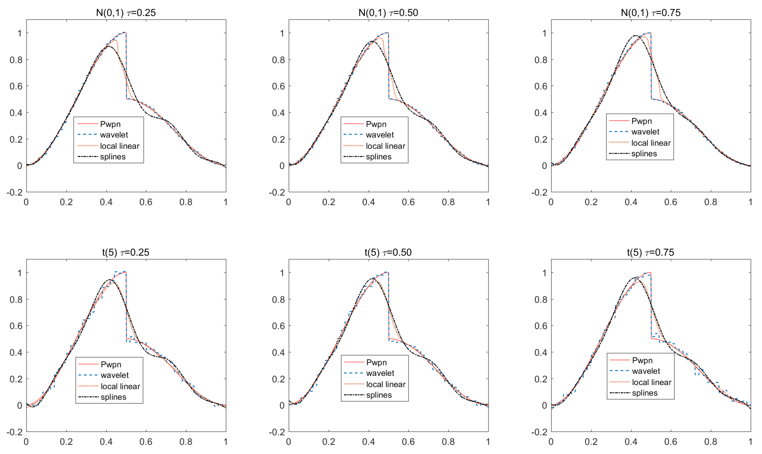
Case 1. Pwpn (piecewise polynomial function): $\beta \left(t\right)=\left[4t^2(3-4t)\right]1_{[0,0.5]\left(t\right)}+[\frac{4}{3}t(4t^2-10t+7)-1.5]1_{(0.5,0.75]}\left(t\right)+\left[\frac{16}{3}t{(t-1)}^2\right]1_{(0.75,1]}\left(t\right)$. The function is generally smooth except for a jump at $t=0.5$.

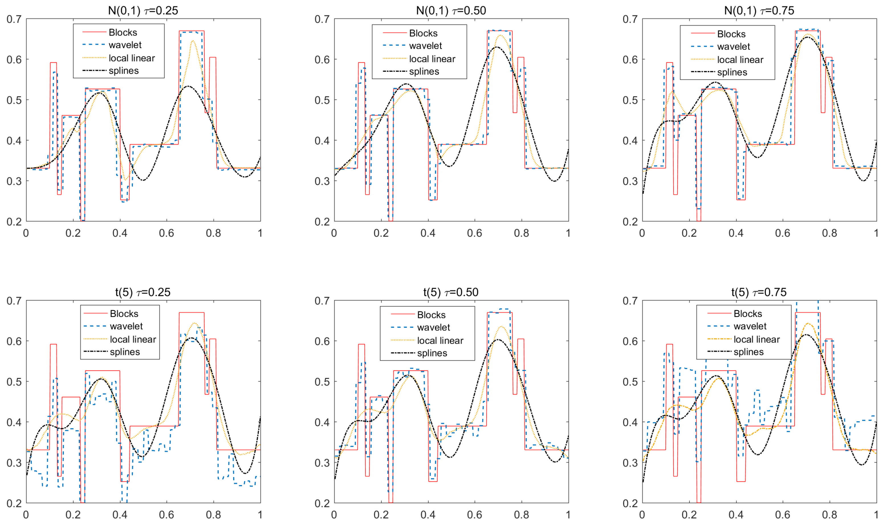
Case 2. Blocks: $\beta \left(t\right)=\frac{0.6}{9.2}\{4\mathrm{ssgn}(t-0.1)-5\mathrm{ssgn}(t-0.13)+3\mathrm{ssgn}(t-0.15)-4\mathrm{ssgn}(t-0.23)+5\mathrm{ssgn}(t-0.25)-4.2\mathrm{ssgn}(t-0.4)+2.1\mathrm{ssgn}(t-0.44)+4.3\mathrm{ssgn}(t-0.65)-3.1\mathrm{ssgn}(t-0.76)+2.1\mathrm{ssgn}(t-0.78)-4.2\mathrm{ssgn}(t-0.81)\}+0.2$, where $\mathrm{ssgn}\left(t\right)=[1+\mathrm{sgn}(t\left)\right]/2$ with $\mathrm{sgn}\left(t\right)=1_{(0,\infty )}\left(t\right)-1_{(-\infty ,0)}\left(t\right)$. It is a step function with many jumps. Many jumps bring difficulties for the local linear and spline smoothing methods.

Pwpn and Blocks are shown in Figure 1 and Figure 2, respectively. In the study, we use the Haar wavelet, which is the simplest of the wavelets. For a given sample size, take $2^m=0.6n^{2/3}$ in the QR-wavelet, h is chosen by “leave-one-out" cross-validation procedures and use the Gaussian kernel $K\left(t\right)=exp(-t^2/2)/\sqrt{2\pi }$ in the QR-local-linear. In the QR-splines, we use three degrees of the piecewise polynomial (cubic splines) and the knots $\lfloor 0.5n^{1/2}logn\rfloor$. The performances of the estimators are evaluated via the mean square error (MSE) based on the 200 repetitions, which is defined by

$$\mathrm{MSE}=\frac{1}{M}\sum _{k=1}^M{({\widehat{\beta }}_{\tau }\left(t_k\right)-\beta \left(t_k\right))}^2,$$

where $\{t_k,k=1,\cdots ,M\}$ is a sequence of regular grid points. These results of MSE for ${\widehat{\beta }}_{\tau }(·)$ are listed in Table 1 for Case I (Pwpn) and Table 2 for Case II (Blocks). The actual functions and their estimated curves for the two cases are depicted in Figure 1 and Figure 2 when $n=300$, and $\tau =0.25$, 0.5 and 0.75, respectively.

Figure 1. The true time-varying coefficient function Papw, and their QR-wavelet, QR-local-linear and QR-splines estimates when $n=300$, and $\tau =0.25$, 0.50 and 0.75 for the errors $N(0,1)$ and $t\left(5\right)$.

Figure 2. The true time-varying coefficient function Blocks and their QR-wavelet, QR-local-linear and QR-splines estimates when $n=300$, and $\tau =0.25$, 0.50 and 0.75 for the errors $N(0,1)$ and $t\left(5\right)$.

Table 1. MSEs of wavelet, local linear and spline smoothing in Case I: Pwpn.

		QR-Wavelet		QR-Local-Linear		QR-Splines
$\mathit{n}$	$\mathit{\tau }$	$\mathit{N}(\mathbf{0},{\mathbf{0.1}}^{\mathbf{2}})$	$\mathit{t}\left(\mathbf{5}\right)$	$\mathit{N}(\mathbf{0},{\mathbf{0.1}}^{\mathbf{2}})$	$\mathit{t}\left(\mathbf{5}\right)$	$\mathit{N}(\mathbf{0},{\mathbf{0.1}}^{\mathbf{2}})$	$\mathit{t}\left(\mathbf{5}\right)$
200	0.10	0.00073	0.02273	0.00644	0.00479	0.01032	0.00824
	0.25	0.00065	0.00125	0.00383	0.00299	0.00859	0.00584
	0.50	0.00062	0.00085	0.00213	0.00293	0.00530	0.00529
	0.75	0.00065	0.00104	0.00293	0.00262	0.00860	0.00532
	0.90	0.00074	0.02208	0.00474	0.00345	0.01011	0.00660
300	0.10	0.00042	0.00966	0.00605	0.00287	0.01049	0.00557
	0.25	0.00040	0.00157	0.00355	0.00271	0.00868	0.00539
	0.50	0.00037	0.00055	0.00197	0.00250	0.00529	0.00524
	0.75	0.00039	0.00141	0.00279	0.00244	0.00867	0.00534
	0.90	0.00041	0.01121	0.00455	0.00254	0.01017	0.00561
500	0.10	0.00011	0.00319	0.00516	0.00262	0.00514	0.00319
	0.25	0.00010	0.00041	0.00311	0.00227	0.00358	0.00309
	0.50	0.00010	0.00026	0.00176	0.00213	0.00303	0.00300
	0.75	0.00010	0.00045	0.00255	0.00221	0.00354	0.00306
	0.90	0.00011	0.00354	0.00411	0.00252	0.00532	0.00339

Table 2. MSEs of wavelet, local linear and spline smoothing in Case II: Blocks.

		QR-Wavelet		QR-Local-Linear		QR-Splines
$\mathit{n}$	$\mathit{\tau }$	$\mathit{N}(\mathbf{0},{\mathbf{0.1}}^{\mathbf{2}})$	$\mathit{t}\left(\mathbf{5}\right)$	$\mathit{N}(\mathbf{0},{\mathbf{0.1}}^{\mathbf{2}})$	$\mathit{t}\left(\mathbf{5}\right)$	$\mathit{N}(\mathbf{0},{\mathbf{0.1}}^{\mathbf{2}})$	$\mathit{t}\left(\mathbf{5}\right)$
200	0.10	0.00573	0.01904	0.01114	0.00714	0.01730	0.00897
	0.25	0.00503	0.00368	0.00661	0.00593	0.00921	0.00778
	0.50	0.00378	0.00347	0.00599	0.00587	0.00803	0.00765
	0.75	0.00418	0.00384	0.00721	0.00613	0.00894	0.00773
	0.90	0.00574	0.02662	0.00865	0.00822	0.01150	0.01086
300	0.10	0.00624	0.01358	0.01059	0.00622	0.01751	0.00777
	0.25	0.00611	0.00553	0.00647	0.00556	0.00925	0.00764
	0.50	0.00484	0.00448	0.00584	0.00567	0.00800	0.00761
	0.75	0.00674	0.00557	0.00704	0.00570	0.00897	0.00775
	0.90	0.00682	0.01421	0.00852	0.00592	0.01139	0.00794
500	0.10	0.00562	0.00426	0.00958	0.00562	0.01541	0.00694
	0.25	0.00385	0.00368	0.00634	0.00528	0.00751	0.00671
	0.50	0.00310	0.00285	0.00557	0.00528	0.00706	0.00669
	0.75	0.00357	0.00325	0.00679	0.00550	0.00757	0.00681
	0.90	0.00408	0.00481	0.00813	0.00545	0.01000	0.00684

From Table 1 and Table 2, we can make the following observations: (i) The MSEs of each time-varying coefficient $\beta (·)$ obtained by wavelet, local linear and spline techniques decrease with increasing the sample size n. The accuracy of QR-wavelet is obviously higher than that of QR-local linear and QR-splines. (ii) All QR methods work well when the random error comes from the t distribution with five freedoms; that is, QR is robust to heavy-tailed data. Based on MSE only, for Pwpn that is generally smooth except for a jump, all three methods perform almost equally well, but for Blocks with many jumps, the QR-wavelet performs better than QR-local linear and QR-splines. (iii) All three methods perform well for different quantile levels, especially for high and low quantile levels ($\tau =0.9$ (high), $\tau =0.1$ (low)). We also conducted some experiments based on the above setting by using least square estimation, and found that their estimators lead to systematic bias, especially at high and low quantile levels. However, QR-wavelet generally performs better than QR-local linear and QR-splines at these extreme quantile levels when there is a large sample size (e.g., $n=500$) and multiple jump points (e.g., Blocks). From Figure 1 and Figure 2, the estimators based on QR-local-linear and QR-splines are not better than those of QR-wavelet. For example, in Pwpn, QR-local linear and QR-splines cannot characterize the shape of the function in the interval $(0.4,0.6)$; in Blocks, they cannot find their jumping points, while QR-wavelet detects these jumping points and represents the localized features of Pwpn and Blocks as a whole. Compared with the local linear and spline methods, the wavelet technique has great advantages in characterizing the local features of underlying curves. Therefore, the QR-wavelet overwhelmingly outperforms the QR-local-linear and QR-splines for the discontinuous/irregular functional coefficients in our time-varying coefficient models.