Efficiency-Oriented MPC: Using Nested Structure to Realize Optimal Operation and Control

Abstract

Optimal operation and control, which can result in the global optimal operation performance of industrial processes, has been a hot topic in recent control strategy designs. However, existing control strategies, such as real-time optimization (RTO), dynamic real-time optimization (DRTO), and economic model predictive control (EMPC), have their own limitations, and they can only generate sub-optimal operation performance. In order to further improve online global operation performance, a new kind of control strategy named efficiency-oriented model predictive control (EfiMPC) is proposed in this paper. The aim of the EfiMPC is discussed first, and then, the ideal EfiMPC strategy with a nested structure is proposed, where the inner layer is the offline construction of an efficiency-oriented terminal region, and the outer layer is the direct optimization of the transient operation performance. This efficiency-oriented terminal region can guarantee a dynamic operation performance in the closed-loop perspective, and a better global operation performance can thus be obtained. A practical EfiMPC strategy, which replaces the offline construction of the efficiency-oriented terminal region with the online optimization of the average dynamic operation performance in the inner layer, is also proposed, and the recursive feasibility as well as the closed-loop stability of practical EfiMPC are discussed. Finally, a CSTR application was used to test the superiority of the proposed EfiMPC strategy, and the simulation results show that EfiMPC can obtain the best global operation performance compared with the other three control strategies; thus, the effectiveness of EfiMPC is demonstrated.

1. Introduction

The optimal operation and control (or optimal operation performance) of industrial processes has been a hot topic in recent control strategy designs, where the optimal operation performance refers to the optimal global performance of the whole system, and this optimal global performance is usually defined by economic objectives [1]. One cornerstone of the optimal operation and control of industrial processes is calculating the optimal operating conditions and maintaining them, despite the presence of different kinds of uncertainties and disturbances [2]. Thus, it is typical to first calculate the optimal steady-state operating condition via a real-time optimization (RTO) layer (calculating the optimal operating conditions), and then, this calculated optimal steady state is passed to the lower advanced control layer (maintaining optimal operating conditions) [3].

Specifically, RTO is an optimization layer that aims to obtain optimal steady states based on an updated rigorous steady-state model at certain intervals [4]. These updated optimal steady-state setpoints are sent to the lower supervisory control layer, which is usually model predictive control [5,6]. Model predictive control (MPC) refers to a class of computer control algorithms that utilize an explicit process model to predict the future responses of a plant [7], and the main advantage of MPC is its explicit constraint handling ability [8,9].

Optimal operation and control are realized by the separation of optimization and control in RTO, but it also has some drawbacks resulting from this separation [10]: (1) before implementing RTO, the controlled system has to be steady enough, which means there is a steady-state waiting time in RTO [11]; (2) there is a model mismatch between the RTO layer and the MPC layer; thus, the MPC may track unreachable setpoints optimized by RTO [12]; (3) the RTO layer focuses only on the steady-state operation, and there may exist better dynamic operations [13].

In order to further improve the global operation performance of the processes, researchers proposed dynamic real-time optimization (DRTO) [14]. As its name implies, DRTO uses a dynamic model to replace the steady-state model used in the RTO layer, and this high-fidelity dynamic model gives DRTO the ability to optimize the transient operation performance [15,16]. Unlike RTO, which only passes the steady states as setpoints to the lower MPC layer, DRTO optimizes a dynamic trajectory based on the global performance of the whole system and then transmits this optimal trajectory to the lower advanced control layer. In this way, the model mismatch problem is fixed in DRTO, and DRTO can directly optimize the optimal dynamic operation rather than the optimal steady-state operation considered in RTO [17]. In other words, DRTO can obtain a better global operation performance than that obtained by RTO.

However, DRTO still preserves the two-layer structure, and the lower control layer, such as nonlinear model predictive control (NMPC), minimizes the tracking errors with respect to the optimized trajectory obtained in the upper DRTO layer [18]. Since there is still a time-scale separation problem between the DRTO layer and the control layer, the real-time disturbances in the processes will make the optimized trajectory sub-optimal during the control, and the NMPC has to track this outdated trajectory until the tracking trajectory is re-optimized at the next DRTO sample instant.

Recently, researchers proposed economic model predictive control (EMPC), which combines the DRTO layer and the control layer into one framework to avoid the time-scale separation problem [19,20]; in this way, EMPC focuses on how to address economic optimization (the operation performance in industrial processes) directly in real time [21]. Unlike the quadratic objective function used in tracking MPC, EMPC incorporates a general cost function that directly accounts for process economics such as process yield or production rate, and this process economics-oriented general objective function gives EMPC the ability to generate optimal dynamic operation performance [22]. In other words, EMPC can determine the operating conditions leading to the optimal operation performance, and the safe operating conditions of the processes can also be guaranteed [23].

The direct responses to the dynamic economic optimization resulting from the general objective function in EMPC will inevitably bring stability issues to the controlled processes [24]. Additional conditions are required for EMPC to guarantee closed-loop stability, and there are mainly two types of common approaches to ensuring stability in the EMPC community: one is the use of the dissipativity condition, and the other is the additional terminal constraints. Dissipativity-based EMPC is terminal-free EMPC, which relies on the turnpike property [25,26], but the turnpike property and dissipativity both have strict requirements on the controlled plant; thus, we mainly focus on the terminal constraint-based EMPC in this paper. Terminal constraints in EMPC can be categorized into three common types: terminal equality-based EMPC [27], terminal region-based EMPC [28], and Lyapunov-based EMPC [29]. However, Lyapunov-based EMPC needs to construct a Lyapunov function, terminal equality-based EMPC needs to steer the terminal state into a pre-determined steady state, which makes the feasible region small, and terminal region-based EMPC ignores the operation performance within the terminal region.

Thus, terminal constraint-based EMPC loses some optimality of the global operation performance because of the terminal conditions, and a better control strategy that can realize a better optimal dynamic operation performance is desired.

To summarize, given a general economic objective function defined in the operational layer, the global operation performance of the whole system can be evaluated (which will be discussed in detail in Section 2). The advantage of RTO is that it separates the optimizing control of the global operation performance into two layers: the upper RTO layer calculates the optimal steady-state operation first, and then the lower control layer tracks this optimized setpoint. In this way, the optimization of the global operation performance in RTO is easy to realize. However, RTO cannot optimize the transient operation performance. DRTO, on the other hand, uses a dynamic model in the RTO layer, which can optimize the transient operation performance, and the global operation performance can thus be improved. However, the time-scale separation of DRTO makes the optimized trajectory sub-optimal in real-time control. EMPC integrates DRTO and the MPC layer to address the time-scale separation problem to further increase the global operation performance, but the additional terminal conditions restrict the improvements of the global operation performance. Thus, the main aim of this study is to address the drawbacks of EMPC to further improve the global operation performance of the controlled system.

In view of the above issues, the main contribution of this paper is to propose a new kind of control strategy named efficiency-oriented model predictive control (EfiMPC), which can further improve the global operation performance of industrial processes. Specifically, EfiMPC is a nested optimization structure where the outer layer mainly focuses on the global performance of the whole system, and the inner layer mainly focuses on the control performance to guarantee the closed-loop stability of the processes. Ideal EfiMPC is first proposed, where the inner layer is the offline construction of an efficiency-oriented terminal region, and then a practical EfiMPC is constructed, where the inner layer is the online optimization of the dynamic operation performance, and the efficiency-oriented terminal region needs not to be explicitly defined in practical EfiMPC. With this nested optimization structure, EfiMPC can realize a better global dynamic operation performance by optimizing control.

The rest of this article is organized as follows. Section 2 presents the problem that efficiency-oriented model predictive control (EfiMPC) tries to address. In Section 3, the details of the proposed EfiMPC are given, and ideal EfiMPC, where the inner layer is calculated offline, and practical EfiMPC, where the inner layer is optimized online, are discussed. The recursive feasibility, as well as the closed-loop stability of practical EfiMPC, is also discussed briefly. Section 4 demonstrates the superiority of the proposed EfiMPC strategy compared to the other three control strategies in a CSTR application. Finally, Section 5 concludes this article.

2. Problem Statement

The problem considered in this paper is the optimization of the operation performance of industrial processes, namely the global performance of the whole system, and to obtain optimal operation performance results from the optimal operation and control of plants with the help of the ideal control strategy. This operation performance is usually evaluated by a general economic objective function $l_P$ defined in the operational layer. Mathematically speaking, the ideal optimizing control problem, which aims to achieve the optimal operation performance, has the following form:

$$\begin{array}{c}{J}_P^{*}=\underset{u_P}{\min }{J}_P\left(u_P;x_0\right)=\underset{u_P}{\min }{{\displaystyle \int }}_{t_0}^{t_f}{l}_P\left(x\left(t\right),u_P\left(t\right)\right)dt,\\ s.t. \dot{x}=f\left(x\left(t\right),u_P\left(t\right)\right),x\left(t_0\right)=x_0\\ x\left(t\right)\in \mathcal{X},u_P\left(t\right)\in \mathcal{U},t_0\le t\le t_f\end{array}$$

(1)

where $x_0$ is the initial state of the system, $u_p$ is the decision variable of the optimization problem (1), $l_P$ is the economic objective function defined in the operational layer representing the instantaneous global performance of the whole system, $f$ is the nonlinear dynamics of the industrial process, and $\mathcal{X}$ and $\mathcal{U}$ are the constraints of the system states and control inputs, respectively.

In Equation (1), $t_0$ is the starting instant of the process operation, and $t_f$ is the ending instant of the process operation. $J_P$ is the global operation performance function of the controlled process over the entire operation interval from $t_0$ to $t_f$, $J_P^{*}$ is the optimal global operation performance, and $u_P^{*}$ is the corresponding optimal input trajectory.

However, optimizing control problem (1) is too idealistic to implement in practice. The main issues are: (1) the optimal solution $u_P^{*}$ to Equation (1) is an offline optimal solution, and thus, the optimality of $u_P^{*}$ will be degraded when disturbances or uncertainties exist during the process operation; (2) the optimization horizon of Equation (1) is the entire operation interval from $t_0$ to $t_f$, which is too large to solve this optimization problem successfully.

In view of these issues, researchers prefer to use a receding horizon strategy to approximate this idealistic optimizing control problem (1). To be specific, short-horizon-based online optimization problems can be used to solve this global optimizing control problem at every sample instant $t_k$, and it is usually denoted as (nonlinear) model predictive control (MPC) with the following typical definition:

$$\begin{array}{c}{J}_k^{*}=\underset{u_k}{\min }{J}_k\left(u_k;x_k\right)=\underset{u_k}{\min }{{\displaystyle \int }}_{t_k}^{t_k+H}{l}_F\left(x\left(t\right),u_k\left(t\right)\right)dt+V_F\left(x_{k+H}\right)\\ s.t.\dot{x}=f\left(x\left(t\right),u_k\left(t\right)\right),x\left(t_k\right)=x_k,x_{k+H}=x\left(t_k+H\right)\\ x\left(t\right)\in \mathcal{X},u_k\left(t\right)\in \mathcal{U},t_k\le t\le t_k+H\\ x_{k+H}\in {\mathcal{X}}_F\end{array}$$

(2)

where $t_k,k=0,1,\dots ,$ represents the current sample instant, $x_k=x\left(t_k\right)$ represents the system state at time instant $t_k$ for brevity, $H$ represents a finite prediction horizon and $x_{k+H}=x\left(t_k+H\right)$ represents the terminal state at the end of the online optimization problem (2); $V_F\left(x_{k+H}\right)$ is a terminal cost and ${\mathcal{X}}_F$ is a terminal constraint, and they are added mainly to guarantee the closed-loop stability of the controlled process; $l_F$ is a stage cost function of the controller aiming to guide the control actions. Usually, this stage cost $l_F$ is typically a penalty function of the tracking error with respect to the setpoint $\left(x_s,u_s\right)$, and this setpoint is obtained from a real-time optimization (RTO) layer implementing the optimization of the steady-state operation performance $l_P\left(x_s,u_s\right)$.

However, unlike the idealistic problem (1), which directly optimizes the global operation performance, the approximation problem (2) focuses only on optimizing the control performance with respect to the optimal steady state $\left(x_s,u_s\right)$ within the prediction horizon $H$, and the local operation performance is a byproduct of maintaining the optimal steady-state operation.

Specifically, in Equation (2), $J_k$ is an open-loop control performance function, $J_k^{*}$ is the optimal control performance, and $u_k^{*}$ is the corresponding optimal control action. At every sample instant $t_k, k=0,1,2,\dots$, MPC will solve the online optimization problem (2) repeatedly, and then the first control action $u_k^{*}\left(t_k\right)$ will be implemented in the plant. The resulting implicit closed-loop input profile is defined as follows:

$$u_C^{*}\left(t\right)=u_k^{*}\left(t_k\right), \mathrm{for}t\in \left[t_k,t_{k+1}\right),k=0,1,2,\dots$$

The closed-loop system controlled by $u_C^{*}\left(t\right)$ has a corresponding global operation performance $J_C^{*}$ evaluated by the economic objective function $l_P$ defined in the operational layer, and its specific value is calculated as follows:

$$J_C^{*}={{\displaystyle \int }}_{t_0}^{t_f}{l}_P\left(x\left(t\right),u_C^{*}\left(t\right)\right)dt$$

Since this operation performance $J_C^{*}$ is realized by the online optimization of problem (2), which aims to optimize the control performance $l_F$, the degree of the approximation of $J_C^{*}$ towards the ideal optimal operation performance $J_P^{*}$ is disappointing. Thus, it is desired to construct a control strategy that can realize optimizing control with a better operation performance $J_E^{*}$, and the efficiency-oriented model predictive control (EfiMPC) proposed in this paper is a promising control strategy that aims to better approximate $J_P^{*}$ by $J_E^{*}$. The term efficiency-oriented can be understood as EfiMPC improving the efficiency of this approximation $\frac{J_E^{*}}{J_P^{*}}\to 1$, where $J_P^{*}$ is determined by the controlled industrial process itself.

3. Efficiency-Oriented Model Predictive Control

3.1. Motivations for Efficiency-Oriented MPC

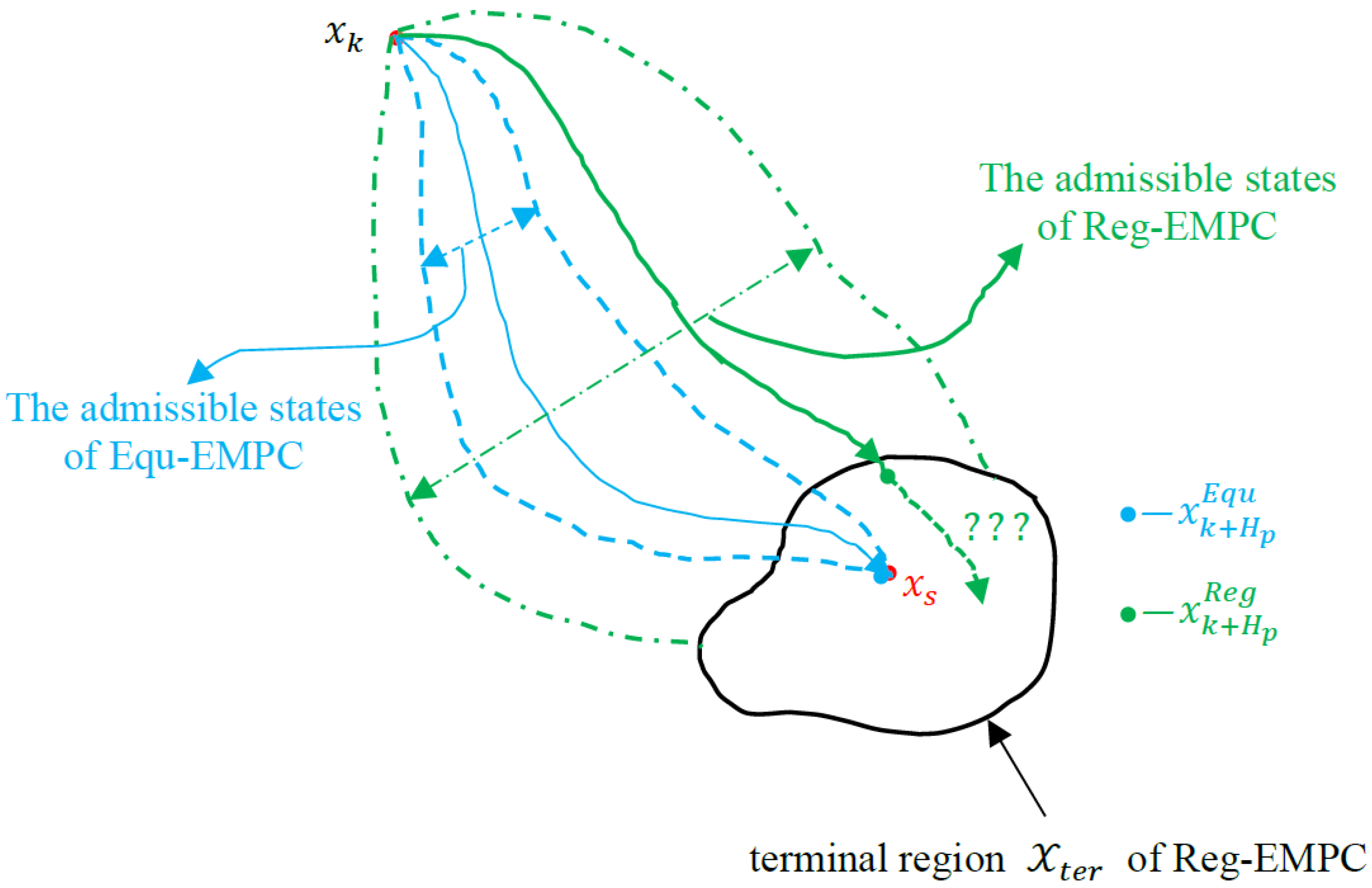
The recently proposed economic MPC (EMPC) strategies, for example, terminal-equality-based EMPC (Equ-EMPC) and terminal-region-based EMPC (Reg-EMPC), can improve the global operation performance of the process operation to some extent, but they have their own limitations that result from their structures. The advantages and disadvantages of Equ-EMPC and Reg-EMPC are briefly illustrated in Figure 1.

In Figure 1, $x_k$ is the system state at the current sample instant $t_k$, and $x_s$ is the optimal steady state in the interior of a terminal region ${\mathcal{X}}_{ter}$, which means $x_s\in {\mathcal{X}}_{ter}$. This optimal steady state $x_s$ is obtained from the following sub-optimization problem:

$$\begin{array}{c}\underset{x_s,u_s}{\mathrm{minimize}} l_P\left(x_s,u_s\right)\\ s.t.f\left(x_s,u_s\right)=0\\ x_s\in {\mathcal{X}}_{ter}\subseteq \mathcal{X},u_s\in \mathcal{U}\end{array}$$

(3)

where $l_P$ is the economic objective defined in the operational layer, $f$ is the dynamic model of the industrial process, and $\mathcal{X}$ and $\mathcal{U}$ are the constraints of the system states and control inputs, respectively. This optimal steady state $x_s$ can be used as the terminal equality constraint to guarantee the closed-loop stability of the controlled system, and the resulting Equ-EMPC is defined as follows:

$$\begin{array}{c}{V}_{Equ}^{*}=\underset{u}{\min }{{\displaystyle \int }}_{t_k}^{t_k+H_p}{l}_P\left(x\left(t\right),u\left(t\right)\right)dt\\ s.t. \dot{x}=f\left(x,u\right)\\ x\left(t\right)\in \mathcal{X},u\left(t\right)\in \mathcal{U},\forall t\in \left[t_k,t_k+H_p\right)\\ x\left(t_k+H_p\right)=x_s\end{array}$$

(4)

where $t_k$ is the current sample instant, $H_p$ is the prediction horizon of the online optimization problem, $f\left(x,u\right)$ is the dynamic model of the controlled process, and $\mathcal{X}$ and $\mathcal{U}$ are the constraints of system states and control inputs, respectively. $x\left(t_k+H_p\right)$ is the terminal state at the end of the optimization horizon, and it is steered into the optimal steady state $x_s$.

Equ-EMPC can optimize the transient operation performance before steady-state operation, and the global operation performance has thus been improved accordingly. However, for the general economic objective function $l_P$ considered in this paper, it is assumed that a better dynamic state $x_{best}\in {\mathcal{X}}_{ter}$ exists that satisfies $l_P\left(x_{best},u_{best}\right)<l_P\left(x_s,u_s\right)$; thus, the optimal dynamic operation is more desirable than the steady-state operation defined by $x_s$. On the other hand, this hard equality constraint $x\left(t_k+H_p\right)=x_s$ restricts the feasible searching space of the control input, and the range of the corresponding admissible control trajectories are reduced accordingly. These admissible states constrained by $x_s$ are denoted by the region within the dashed-blue lines in Figure 1, and the optimization of the transient operation performance is degraded because of this smaller feasible region.

To summarize, the limitations of Equ-EMPC with respect to the operation performance are mainly twofold: (1) it cannot lead to the optimal dynamic operation based on a general objective function $l_P$; (2) the transient operation performance before stabilizing into the optimal steady state $x_s$ is also degraded because of a smaller feasible region.

As for Reg-EMPC, the terminal region ${\mathcal{X}}_{ter}$ illustrated in Figure 1 helps to enlarge the feasible space of the admissible trajectories denoted by the region within the dashed-green lines; thus, the transient operation performance of Reg-EMPC is better than that of the Equ-EMPC. The detailed definition of Reg-EMPC is as follows:

$$\begin{array}{c}{V}_{Reg}^{*}=\underset{u}{\min }{{\displaystyle \int }}_{t_k}^{t_k+H_p}{l}_P\left(x\left(t\right),u\left(t\right)\right)dt\\ s.t. \dot{x}=f\left(x,u\right)\\ x\left(t\right)\in \mathcal{X},u\left(t\right)\in \mathcal{U},\forall t\in \left[t_k,t_k+H_p\right)\\ x\left(t_k+H_p\right)\in {\mathcal{X}}_{ter}\end{array}$$

(5)

where the definitions of most parameters are the same as those defined in Equation (4), and ${\mathcal{X}}_{ter}$ is the terminal region where $x_s\in {\mathcal{X}}_{ter}$.

In Reg-EMPC, it is assumed that there exists a local control policy $𝒽\left(·\right)$ within the terminal region ${\mathcal{X}}_{ter}$ such that any states $x\in {\mathcal{X}}_{ter}$ can be controlled to stay within this terminal region. This local control policy is used mainly for the considerations of the recursive feasibility and the closed-loop stability, while the operation performance within this terminal region has been ignored. As shown in Figure 1, Reg-EMPC will steer the terminal state $x\left(t_k+H_p\right)$ into the terminal region ${\mathcal{X}}_{ter}$, but the future behaviors of the system with respect to the operation performance are uncertain; thus, it is not safe to say that the closed-loop operation performance of Reg-EMPC is definitely better than that of Equ-EMPC. Instead, it can only be concluded that the open-loop transient operation performance of Reg-EMPC is better than that of Equ-EMPC.

To summarize, Reg-EMPC can guarantee a better open-loop transient operation performance than Equ-EMPC, but the closed-loop operation performance of Reg-EMPC is uncertain because of the use of the terminal region ${\mathcal{X}}_{ter}$. In other words, Reg-EMPC can directly optimize the local operation performance, but it is unable to directly optimize the global operation performance.

Drawbacks, on the other hand, always mean there are chances for improvement. The newly proposed control strategy in this paper mainly aims to address the limitations that exist in Equ-EMPC and Reg-EMPC. Briefly speaking, efficiency-oriented model predictive control (EfiMPC) tries to (1) improve the open-loop operation performance, which means enlarging the admissible state region for optimization, and (2) improve the closed-loop operation performance, which means guaranteeing the operation performance within the terminal region ${\mathcal{X}}_{ter}$ to generate a better global operation performance.

3.2. Ideal Efficiency-Oriented Model Predictive Control

Ideal efficiency-oriented MPC (ideal EfiMPC) is defined as follows:

$$\begin{array}{c}{V}_{I-Efi}^{*}=\underset{u}{\min }{{\displaystyle \int }}_{t_k}^{t_k+H_p}{l}_P\left(x\left(t\right),u\left(t\right)\right)dt\\ s.t. \dot{x}=f\left(x,u\right)\\ x\left(t\right)\in \mathcal{X},u\left(t\right)\in \mathcal{U},\forall t\in \left[t_k,t_k+H_p\right)\\ x\left(t_k+H_p\right)\in {\mathcal{X}}_{ter}^{Efi}\subseteq {\mathcal{X}}_{ter}\end{array}$$

(6)

where the definitions of most parameters are the same as those defined in Equation (5), ${\mathcal{X}}_{ter}^{Efi}$ is an efficiency-oriented terminal region, which is a subset of the control forward-invariant set ${\mathcal{X}}_{ter}$, and the optimal steady state $x_s$ is in the interior of this ${\mathcal{X}}_{ter}^{Efi}$. A corresponding local control policy $𝒽\left(·\right)$ as defined in Reg-EMPC can also guarantee stabilization within this efficiency-oriented terminal region ${\mathcal{X}}_{ter}^{Efi}$.

The specific definition of ${\mathcal{X}}_{ter}^{Efi}$ is as follows:

$${\mathcal{X}}_{ter}^{Efi}=\left\{x\right|\forall x\left(t_0\right)\in {\mathcal{X}}_{ter}^{Efi},\exists u\left(t_0;t_{ter}\right) such that x\left(t_{ter}\right)=x_s and Ave\left(X_{ter}\right)\le l_P\left(x_s,u_s\right)\}$$

(7)

where $u\left(t_0;t_{ter}\right)=u\left(t\right),t\in \left[t_0,t_{ter}\right)$ is a feasible control sequence that can steer the state $x\left(t_0\right)\in {\mathcal{X}}_{ter}^{Efi}$ into the optimal steady state $x_s\in {\mathcal{X}}_{ter}^{Efi}$. In other words, $x_s$ is in the interior of ${\mathcal{X}}_{ter}^{Efi}$, and $x_s$ can be reached from any state within this efficiency-oriented terminal region. $Ave\left(X_{ter}\right)$ is the average dynamic operation performance of the system dynamics controlled by $u\left(t_0;t_{ter}\right)$, and it satisfies:

$$Ave\left(X_{ter}\right)=\frac{{{\displaystyle \int }}_{t_0}^{t_{ter}}{l}_P\left(x\left(t\right),u\left(t\right)\right)dt}{t_{ter}-t_0}.$$

This inequality condition $ave\left(X_{ter}\right)\le l_P\left(x_s,u_s\right)$ guarantees that the dynamic operation performance controlled by ideal EfiMPC is at least no worse than the optimal steady-state operation (minimum implies optimum in this paper).

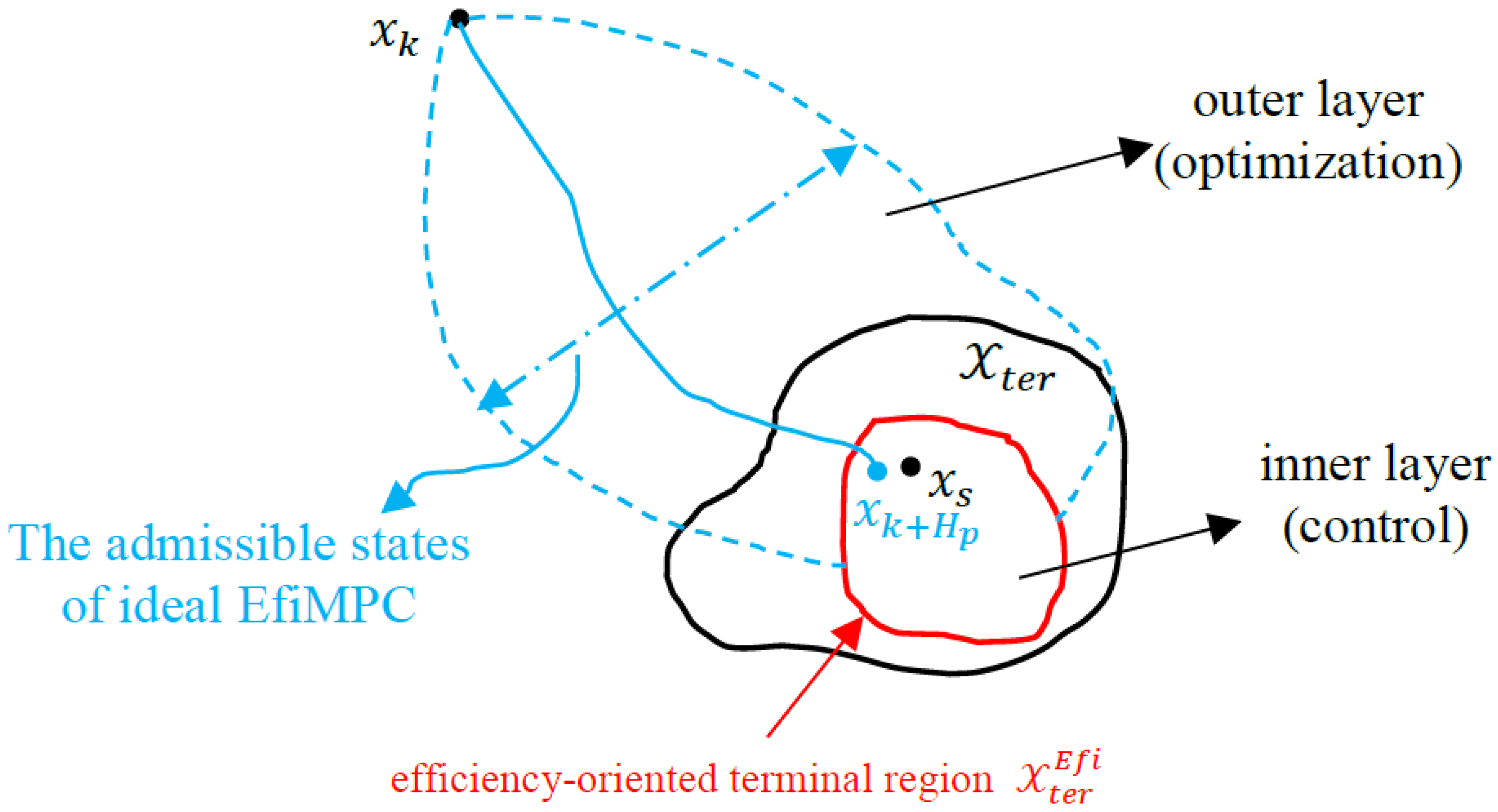
The brief ideas of ideal EfiMPC are illustrated in Figure 2, and its superiorities over Equ-EMPC and Reg-EMPC are as follows:

(1)

Since $x_s\in {\mathcal{X}}_{ter}^{Efi}$, the feasible region of the admissible states of ideal EfiMPC is greater than that of Equ-EMPC; thus, the transient operation performance of ideal EfiMPC evaluated by the economic objective $l_P$ is better than that of Equ-EMPC. In addition, because the average dynamic performance of $Ave\left(X_{ter}\right)$ is at least no worse than the optimal steady-state operation, ideal EfiMPC can also realize a better dynamic operation, and the closed-loop operation performance is thus better than that of Equ-EMPC.

(2)

Reg-EMPC focuses mainly on the improvement of the local operation performance within the prediction horizon $H_p$, and the global operation performance of Reg-EMPC cannot be guaranteed. On the contrary, ideal EfiMPC can guarantee the global operation performance within the efficiency-oriented terminal region ${\mathcal{X}}_{ter}^{Efi}$ with the help of the average dynamic performance condition $Ave\left(X_{ter}\right)\le l_P\left(x_s,u_s\right)$; thus, the closed-loop performance of Reg-EMPC evaluated by the economic objective cannot be guaranteed, while ideal EfiMPC can definitely generate a better dynamic operation performance.

The performance of ideal EfiMPC is heavily dependent on the construction of the efficiency-oriented terminal region ${\mathcal{X}}_{ter}^{Efi}$. As shown in Figure 2, the state trajectory from $x_k$ to $x_{k+H_p}$ aims to improve the transient operation performance within the prediction horizon $H_p$, and it can be regarded as an outer layer focusing on the optimization perspective; the terminal state $x_{k+H_p}$ is controlled into an efficiency-oriented terminal region ${\mathcal{X}}_{ter}^{Efi}$ which relates the local operation performance with the global operation performance, and it can be regarded as an inner layer focusing on the control perspective.

In essence, ideal EfiMPC can be regarded as a nested optimization structure based on the construction of an efficiency-oriented terminal region ${\mathcal{X}}_{ter}^{Efi}$ in its inner layer as follows:

$$\begin{array}{c}{V}_{I-Efi}^{*}=\underset{u}{\min }{{\displaystyle \int }}_{t_k}^{t_k+H_p}{l}_P\left(x\left(t\right),u\left(t\right)\right)dt\\ s.t. \dot{x}=f\left(x,u\right)\\ x\left(t\right)\in \mathcal{X},u\left(t\right)\in \mathcal{U},\forall t\in \left[t_k,t_k+H_p\right)\\ x\left(t_k+H_p\right)\in {\mathcal{X}}_{ter}^{Efi}\subseteq {\mathcal{X}}_{ter} \\ s.t. {\mathcal{X}}_{ter}^{Efi}=\left\{x\right|\forall x\left(t_0\right)\in {\mathcal{X}}_{ter}^{Efi},\exists u\left(t_0;t_{ter}\right) such that x\left(t_{ter}\right)=x_s and Ave\left(X_{ter}\right)\le l_P\left(x_s,u_s\right)\}\end{array}$$

(8)

where the inner layer is an offline construction of ${\mathcal{X}}_{ter}^{Efi}$ in ideal EfiMPC, and ${\mathcal{X}}_{ter}^{Efi}$ is defined in Equation (7). This nested structure integrates the optimization and control into one framework, where the outer layer aims to optimize the transient operation performance by $u\left(t\right),t\in \left[t_k,t_k+H_p\right)$, and the inner layer aims to control the closed-loop system while guaranteeing the dynamic operation performance, which is at least no worse than the optimal steady-state operation.

Remark 1.

When${\mathcal{X}}_{ter}^{Efi}=\left\{x_s\right\}$, ideal EfiMPC will be degraded into Equ-EMPC, and when${\mathcal{X}}_{ter}^{Efi}={\mathcal{X}}_{ter}$, ideal EfiMPC will be degraded into Reg-EMPC. Thus, it is not surprising that ideal EfiMPC can outperform both Equ-EMPC and Reg-EMPC because they can be regarded as two extremes of ideal EfiMPC.

Ideally, if one can obtain an optimal ${\mathcal{X}}_{ter}^{Efi}$ by offline construction, ideal EfiMPC can generate the optimal dynamic operation performance as expected. However, this ${\mathcal{X}}_{ter}^{Efi}$ is a problem-dependent subset that has to be constructed for every control problem, and the construction itself is not a simple task. Indeed, we do not need such an optimal efficiency-oriented terminal region ${\mathcal{X}}_{ter}^{Efi}$ where every element $x\in {\mathcal{X}}_{ter}^{Efi}$ in it can generate a promising dynamic operation; instead, we only need to find one feasible dynamic operation that outperforms steady-state operation. Of course, we want this “feasible” dynamic operation to perform as best as possible, and this leads to an online optimization of the dynamic operation within ${\mathcal{X}}_{ter}^{Efi}$. Thus, the offline construction of ${\mathcal{X}}_{ter}^{Efi}$ in the inner layer in ideal EfiMPC can be realized by an online optimization problem. This kind of nested control strategy is denoted as “practical efficiency-oriented MPC” (practical EfiMPC), and it is discussed in detail in the following subsection.

3.3. Practical Efficiency-Oriented Model Predictive Control

Practical efficiency-oriented MPC (practical EfiMPC) is defined as follows:

$$\begin{array}{c}{V}_{P-Efi}^{*}=\underset{u_{Hp},u_{H_{ter}}}{\min }{{\displaystyle \int }}_{t_k}^{t_k+H_p}{l}_P\left(x\left(t\right),u_{Hp}\left(t\right)\right)dt+V_P\left(x\left(t_k+H_p\right)\right)\\ s.t. \dot{x}=f\left(x,u_{Hp}\right)\\ x\left(t\right)\in {\mathcal{X}}_{out},u_{Hp}\left(t\right)\in {\mathcal{U}}_{out},\forall t\in \left[t_k,t_k+H_p\right)\\ x\left(t_k+H_p\right)\in {\mathcal{X}}_{ter}\\ V_P\left(x\left(t_k+H_p\right)\right)=\{\begin{array}{c}0, V_{ave}\le l_e\left(x_s,u_s\right)\\ \infty , otherwise \end{array}\\ V_{ave}=\underset{u_{H_{ter}}}{\min }\frac{1}{H_{ter}}{{\displaystyle \int }}_{t_p}^{t_p+H_{ter}}{l}_P\left(x\left(t\right),u_{H_{ter}}\left(t\right)\right)dt\\ s.t. \dot{x}=f\left(x,u_{H_{ter}}\right),x\left(t_p\right)=x\left(t_k+H_p\right)\\ x\left(t\right)\in {\mathcal{X}}_{in},u_{H_{ter}}\left(t\right)\in {\mathcal{U}}_{in},\forall t\in \left[t_p,t_p+H_{ter}\right)\\ x\left(t_p+H_{ter}\right)=x_s\end{array}$$

(9)

where the definitions of most parameters are the same as those defined in Equation (8), $H_p$ is the prediction horizon of the outer level optimization problem, $u_{Hp}$ is the decision variable of the outer level, $x\left(t_k+H_p\right)$ is the terminal state of the outer level, which plays the role of a connecting parameter transmitting the information between the outer level and the inner level, and $V_P$ is the optimizing control parameter indicating whether a better dynamic operation exists. Its specific value depends on $V_{ave}$, which is the average dynamic operation performance of the inner level. Specifically, if the value of $V_{ave}$ is better (smaller in this paper) than the optimal steady-state operation $l_e\left(x_s,u_s\right)$, then $V_P$ is set to be zero to accept this promising dynamic operation performance; otherwise, $V_P$ is set to infinity to indicate that the local performance resulting from $u_{Hp}$ is not acceptable from the perspective of the global operation performance, and this disappointing dynamic operation has to be rejected. $H_{ter}$ is the prediction horizon of the inner level optimization problem, and $u_{H_{ter}}$ is the decision variable of the inner level that can steer the system state into the optimal steady state $x_s\in {\mathcal{X}}_{ter}^{Efi}$.

In practical EfiMPC, ${\mathcal{X}}_{ter}^{Efi}$ is an implicitly defined efficiency-oriented terminal region: if the optimizing control parameter $V_P=0$, it implies that $x\left(t_k+H_p\right)$ falls into an efficiency-oriented terminal region, and the dynamic operation performance is better than the optimal steady-state operation; otherwise, it implies that $x\left(t_k+H_p\right)$ does not belong to any efficiency-oriented terminal region, and the performance of the optimized dynamic operation is poor. In addition, the control actions $u_{Hp}$ and $u_{H_{ter}}$ in practical EfiMPC are both piece-wise constant control sequences, which means $u\left(𝓉\right)=u\left(t_k\right), \mathrm{for}𝓉\in \left[t_k,t_{k+1}\right)$.

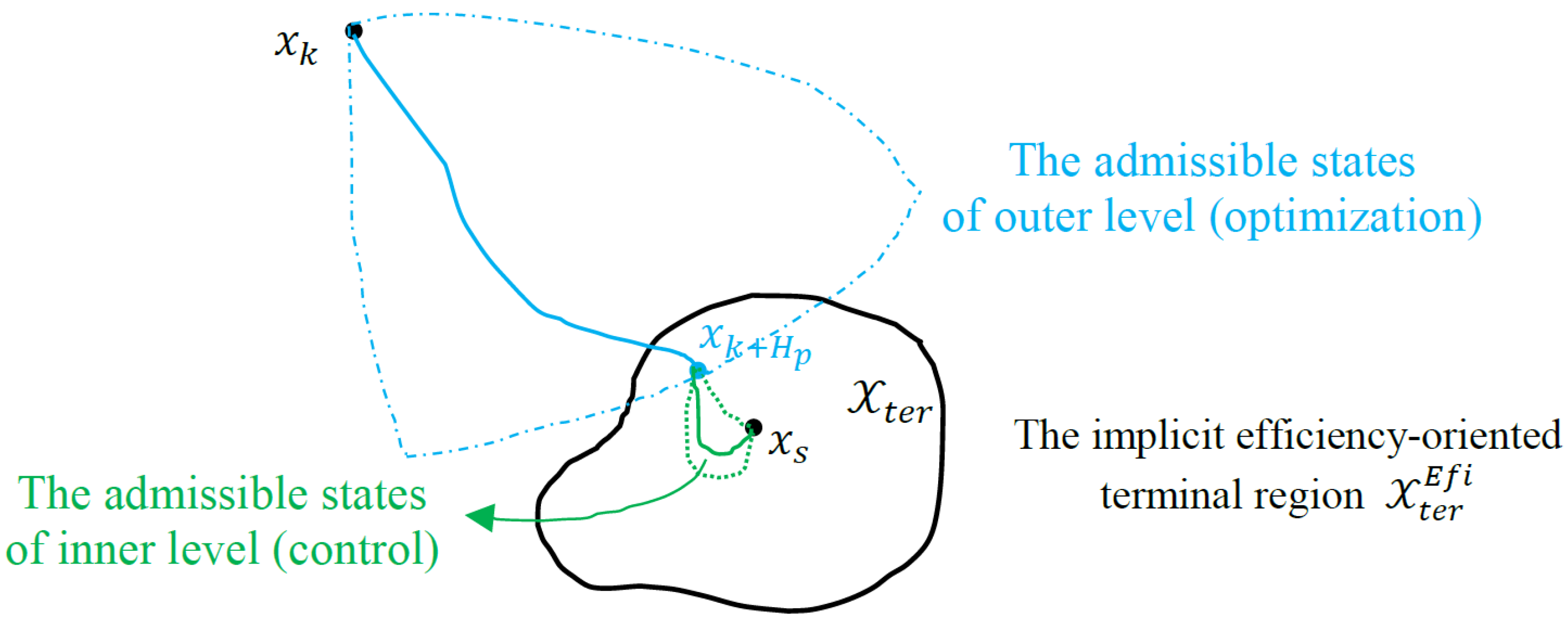
The brief ideas of practical EfiMPC are illustrated in Figure 3. As shown in Figure 3, the admissible states of the outer level are not constrained by the control-oriented equality constraint $x_s$; thus, practical EfiMPC can optimize the transient operation performance to a larger extent. While in the inner level, the control-oriented equality constraint $x\left(t_p+H_{ter}\right)=x_s$ will shrink the range of the admissible states, and the operation performance suffers as a result. In this sense, the main functions of these two levels are different: the outer level focuses mainly on improving the operation performance within the prediction horizon $H_p$, while the inner level focuses mainly on satisfying the control performance to steer the system into $x_s$. The terminal state $x\left(t_k+H_p\right)$ at the outer level is the connecting parameter between the two nested levels; it is the result of the operation performance optimization of the outer level, and then it becomes the starting point of the inner level. At the inner level, the system state is steered into $x_s$, and the dynamic operation performance is also optimized along the system trajectory.

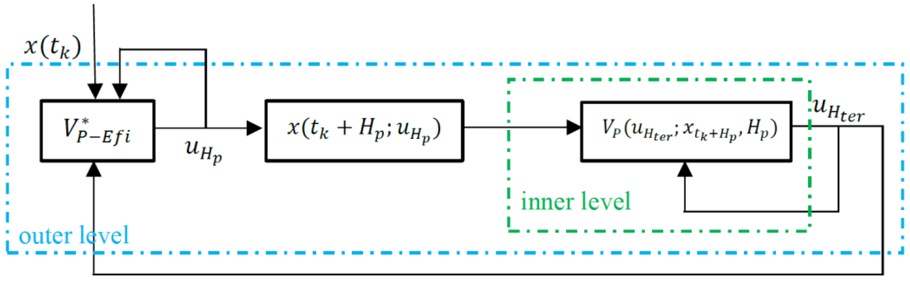
The nested structure of practical EfiMPC is illustrated in Figure 4. The dynamic operation performance of the inner level sends feedback information to the outer level: if the average dynamic operation performance is better than the optimal steady-state operation, it is implied that the controller finds a better dynamic operation; otherwise, the steady-state operation is the best operation for the controlled process. If the optimal solution to practical EfiMPC (9) is $V_{P-Efi}^{*}=\infty$, which means that a better dynamic operation does not exist, then practical EfiMPC will update the terminal region ${\mathcal{X}}_{ter}$ to execute the optimal steady-state operation. The update mechanism is as follows:

$${\mathcal{X}}_{ter}=\{\begin{array}{c}{x}_s, if V_{P-Efi}^{*}=\infty \\ {\mathcal{X}}_{ter}, otherwise \end{array}$$

Remark 2.

With the help of the update mechanism of the terminal region${\mathcal{X}}_{ter}$, practical EfiMPC can intelligently distinguish whether the controlled process has a better dynamic operation than the optimal steady-state operation. If such a better dynamic operation based on the current system state does not exist, practical EfiMPC will be degraded into Equ-EMPC, and the online optimization problem will be re-optimized with the updated terminal region${\mathcal{X}}_{ter}=\left\{x_s\right\}$; otherwise, practical EfiMPC will obtain an optimal dynamic operation to generate the optimal global dynamic operation performance.

The recursive feasibility and the closed-loop stability of practical EfiMPC are discussed briefly as follows. At the current sample instant $t_k$, assume that the practical EfiMPC problem (9) has an optimal solution $u_{*}^k=\left\{u_{H_p,*}^k,u_{H_{ter},*}^k\right\}$, where

$$u_{H_p,*}^k=\left\{u_{H_p,*}^k\left(0\right),u_{H_p,*}^k\left(1\right),\dots ,u_{H_p,*}^k\left(H_p-1\right)\right\},$$

and

$$u_{H_{ter},*}^k=\left\{u_{H_{ter},*}^k\left(0\right),u_{H_{ter},*}^k\left(1\right),\dots ,u_{H_{ter},*}^k\left(H_{ter}-1\right)\right\}.$$

At the next sample instant $t_{k+1}$, there must exist a feasible solution $u_f^{k+1}=\left\{u_{H_p,f}^{k+1},u_{H_{ter},f}^{k+1}\right\}$ such that

$$u_{H_p,f}^{k+1}=\left\{u_{H_p,*}^k\left(1\right),u_{H_p,*}^k\left(2\right),\dots ,u_{H_p,*}^k\left(H_p-1\right),u_{H_{ter},*}^k\left(0\right)\right\},$$

and

$$u_{H_{ter},f}^{k+1}=\left\{u_{H_{ter},*}^k\left(1\right),u_{H_{ter},*}^k\left(2\right),\dots ,u_{H_{ter},*}^k\left(H_{ter}-1\right),u_s\right\}.$$

where $u_s$ is the optimal steady-state control action satisfying $f\left(x_s,u_s\right)=0$.

Since feasibility at sample instant $t_k$ guarantees the feasibility at the next sample instant $t_{k+1}$ and by backward recursion and induction, practical EfiMPC is recursively feasible if it is initially feasible.

The recursive feasibility of practical EfiMPC guarantees that there always exists a feasible solution to the problem Equation (9); thus, it is implied that the system states $x\left(t_k\right),k=0,1,\dots$ can be steered into $x_s$ within $\left(H_p+H_{ter}\right)$ steps. These steerable states form a reachable set ${\mathcal{X}}_R$, where the optimal steady state $x_s$ is reachable from any state $x\in {\mathcal{X}}_R$ in it. Let the initial state satisfy $x\left(t_0\right)\in {\mathcal{X}}_R$, then $x\left(t\right)\in {\mathcal{X}}_R, \forall t\ge t_0$; thus, the system states controlled by practical EfiMPC will be kept in this reachable set ${\mathcal{X}}_R$, and the closed-loop stability with respect to ${\mathcal{X}}_R$ is guaranteed.

4. Results and Discussion

4.1. Application to a Chemical Process Example

In this section, a chemical process example from [30] is used to demonstrate the effectiveness of the proposed practical efficiency-oriented model predictive control (practical EfiMPC or just EfiMPC for brevity in this simulation section), and the simulation results of practical EfiMPC are compared with traditional tracking MPC (TMPC), equality-constraint-based economic MPC (Equ-EMPC), and region-constraint-based economic MPC (Reg-EMPC) control strategies.

Specifically, the chemical process considered in this paper is the oxidation of ethylene to ethylene oxide in a non-isothermal continuously stirred tank reactor (CSTR). The CSTR process is defined by the following three complex reactions:

$$\begin{gathered} C_2{H}_4+\frac{1}{2}{O}_2\to C_2{H}_{4}O \\ {C}_2{H}_4+3O_2\to 2C{O}_2+2H_{2}O \\ {C}_2{H}_{4}O+\frac{5}{2}{O}_2\to 2C{O}_2+2H_{2}O \end{gathered}$$

(10)

The dimensionless equation representing this CSTR application is $\dot{x}=f\left(x,u\right)$, which has the following specific definitions [31,32]:

$$\begin{array}{c}{\dot{x}}_1=u_1\left(1-x_1{x}_4\right)\\ {\dot{x}}_2=u_1\left(u_2-x_2{x}_4\right)-A_1{e}^{{\gamma }_1/x_4}{\left(x_2{x}_4\right)}^{0.5}-A_2{e}^{{\gamma }_2/x_4}{\left(x_2{x}_4\right)}^{0.25}\\ {\dot{x}}_3=-u_1{x}_3{x}_4+A_1{e}^{{\gamma }_1/x_4}{\left(x_2{x}_4\right)}^{0.5}-A_3{e}^{{\gamma }_3/x_4}{\left(x_2{x}_4\right)}^{0.5}\\ {\dot{x}}_4=\frac{u_1}{x_1}\left(1-x_4\right)+\frac{B_1}{x_1}{e}^{{\gamma }_1/x_4}{\left(x_2{x}_4\right)}^{0.5}+\frac{B_2}{x_1}{e}^{{\gamma }_2/x_4}{\left(x_2{x}_4\right)}^{0.25}+\frac{B_3}{x_1}{e}^{{\gamma }_3/x_4}{\left(x_2{x}_4\right)}^{0.5}-\frac{B_4}{x_1}\left(x_4-T_c\right)\end{array}$$

(11)

In Equation (11), the constant parameters and their specific values are as follows [30]: ${\gamma }_1=-8.13$, ${\gamma }_2=-7.12$, ${\gamma }_3=-11.07$, $A_1=92.80$, $A_2=12.66$, $A_3=2412.71$, $B_1=7.32$, $B_2=10.39$, $B_3=2170.57$, $B_4=7.02,$ and $T_{\mathrm{c}}=1.0$. In addition, the dimensionless state variables $x_1,x_2,x_3$, and $x_4$ represent the dimensionless gas density, ethylene concentration, ethylene oxide concentration, and temperature in the reactor, respectively; $u_1,u_2$ are control inputs, where $u_1$ represents the feed volumetric flow rate, and $u_2$ represents the concentration of ethylene in the feed.

The aim of this CSTR application is to maximize the global operation performance $P\left(t_0,t_f\right)$ over the whole process operation from the starting instant $t_0$ to the ending instant $t_f$, and it can be defined by the minimization problem as follows:

$$\begin{gathered} \underset{u}{\max }P\left(t_0,t_f\right)=-\underset{u}{\min }P\left(t_0,t_f\right)=\underset{u}{\min }-P\left(t_0,t_f\right)=\underset{u}{\min }{{\displaystyle \int }}_{t_0}^{t_f}-l_P\left(t\right)dt \\ \mathrm{s}.\mathrm{t}.C_r={{\displaystyle \int }}_{t_0}^{t_f}{u}_1\left(t\right)u_2\left(t\right)dt\le C_{fs} \end{gathered}$$

(12)

where $C_r$ represents the amount of the reactant feedstock during the CSTR process operation, and it is limited by the inventory constraint $C_{fs}$. $l_P\left(t\right)$ is the instantaneous operation performance defined in the operational layer that represents the yield of oxide, and it has the following form as defined in [30]:

$$l_P\left(t\right)=l_P^{CSTR}\left(x\left(t\right),u\left(t\right)\right)=u_1\left(t\right)x_3\left(t\right)x_4\left(t\right)$$

(13)

Due to the actuator limitations, the control actions $u$ are constrained by $0.0704\le u_1\le 0.7042$, $0.2465\le u_2\le 2.4648$. The CSTR process is assumed to be initialized at the initial state $x_0={\left[0.9,1.5,0.2,0.8\right]}^T$, and a sample interval ${\mathsf{\Delta }\mathrm{t}}_{\mathrm{sam}}=1s$ is used in this simulation. The first-order Runge–Kutta numerical integration method was used to obtain the discrete model $f_d$ from Equation (11), and the integration step used here is $h_u={10}^{-2}$. The feedstock constraint defined in Equation (12) satisfies $C_{fs}=0.175\left(t_f-t_0\right)$. In addition, $x_s={\left[0.9956,1.7511,0.2511,1.0043\right]}^T$ represents the optimal steady state, and $u_s={\left[0.0704,2.4648\right]}^T$ is the corresponding optimal control input.

The practical EfiMPC strategy for this CSTR application is defined as follows:

$$\mathrm{EfiMPC}:V_{P-Efi}^{*}=\underset{u_{Hp},u_{H_{ter}}}{\min }{{\displaystyle \int }}_{t_k}^{t_k+H_p}{l}_P\left(x\left(t\right),u_{Hp}\left(t\right)\right)dt+V_P\left(x\left(t_k+H_p\right)\right)$$

(14)

$$s.t. \mathrm{Equation} \left(11\right),\forall t\in \left[t_k,t_k+H_p\right)$$

(14a)

$$0.0704\le u_{Hp,1}\left(t\right)\le 0.7042,t_k\le t\le t_k+H_p$$

(14b)

$$0.2465\le u_{Hp,2}\left(t\right)\le 2.4648,t_k\le t\le t_k+H_p$$

(14c)

$${{\displaystyle \int }}_{t_k}^{t_k+H_p}{u}_{Hp,1}\left(t\right)u_{Hp,2}\left(t\right)dt\le 0.175H_p$$

(14d)

$$x\left(t_k+H_p\right)\in {\mathcal{X}}_{ter}=B_{{\delta }_p}\left(x_s\right)=\left\{x|\Vert x-x_s\Vert {}^2\le {\delta }_p\right\}$$

$$V_P\left(x\left(t_k+H_p\right)\right)=\{\begin{array}{c}0, V_{ave}\le l_e\left(x_s,u_s\right)\\ \infty , otherwise \end{array}$$

$$V_{ave}=\underset{u_{H_{ter}}}{\min }\frac{1}{H_{ter}}{{\displaystyle \int }}_{t_p}^{t_p+H_{ter}}{l}_P\left(x\left(t\right),u_{H_{ter}}\left(t\right)\right)dt$$

$$s.t. x\left(t_p\right)=x\left(t_k+H_p\right)$$

$$\mathrm{Equation} \left(11\right),\forall t\in \left[t_p,t_p+H_{ter}\right)$$

$$0.0704\le u_{H_{ter},1}\left(t\right)\le 0.7042,\forall t\in \left[t_p,t_p+H_{ter}\right)$$

$$0.2465\le u_{H_{ter},2}\left(t\right)\le 2.4648 ,\forall t\in \left[t_p,t_p+H_{ter}\right)$$

$$x\left(t_p+H_{ter}\right)=x_s$$

where most of the parameters are defined the same as those in Equation (9), Equation (11) is the dynamic model of the CSTR process, $B_{{\delta }_p}\left(x_s\right)$ is a ${\delta }_p$-neighborhood of the optimal steady state $x_s$, and ${\Vert x\Vert }^2$ is a norm computation satisfying ${\Vert x\Vert }^2=\sqrt{x^2}$.

The comparative control strategies TMPC, Equ-EMPC, and Reg-EMPC for controlling this CSTR application are defined as follows:

$$\begin{gathered} \mathrm{TMPC}:V_{TMPC}^{*}=\underset{u}{\min }{{\displaystyle \int }}_{t_k}^{t_k+H_p}{\Vert x\left(t\right)-x_s\Vert }_Q^2+u\left(t\right)-{u_s\Vert }_R^{2}dt \\ s.t.\mathrm{Equations} \left(14\mathrm{a}–\mathrm{d}\right) \end{gathered}$$

(15)

$$\begin{gathered} \mathrm{Equ}-\mathrm{EMPC}:V_{Equ}^{*}=\underset{u}{\min }{{\displaystyle \int }}_{t_k}^{t_k+H_p}-u_1\left(t\right)x_3\left(t\right)x_4\left(t\right)dt \\ s.t.\mathrm{Equations} \left(14\mathrm{a}–\mathrm{d}\right) \\ x\left(t_k+H_p\right)-x_s=0 \end{gathered}$$

(16)

$$\begin{gathered} \mathrm{Reg}-\mathrm{EMPC}:V_{Reg}^{*}=\underset{u}{\min }{{\displaystyle \int }}_{t_k}^{t_k+H_p}-u_1\left(t\right)x_3\left(t\right)x_4\left(t\right)dt \\ s.t.\mathrm{Equations} \left(14\mathrm{a}–\mathrm{d}\right) \\ {\Vert x\left(t_k+H_p\right)-x_s\Vert }^2\le {\delta }_R \end{gathered}$$

(17)

where $Q$ and $R$ are symmetric positive semi-definite weighting matrices, and ${\delta }_R$ is a positive scalar value. In Equation (15), the setpoint $\left(x_s,u_s\right)$ is optimized and passed by the real-time optimization (RTO) layer; thus, the TMPC strategy (15) also represents an RTO algorithm.

Remark 3.

Some readers may be confused that the comparative control strategies (14)–(17) target different behaviors by their corresponding objective functions and constraints. However, indeed, comparisons among these control strategies are fair because the controlled system dynamics were used to calculate the same closed-loop operation performance$L_P={{\displaystyle \int }}_{t_0}^{t_f}-l_P\left(x\left(t\right),u\left(t\right)\right)dt$in the simulation. In addition, the values of$L_p$indicate the superiorities of the comparative control strategies.

4.2. Simulation Results

The parameters of the simulations in this paper are defined as follows: $Q=diag\left(\left[1,1,1,1\right]\right)$, $R=diag\left(\left[1,1\right]\right)$, $t_f=50$, ${\delta }_p=1$, ${\delta }_R=0.1$, $H_p=10$, $H_{ter}=10$, $x_0={\left[0.9,1.5,0.2,0.8\right]}^T$, $x_s={\left[0.9956,1.7511,0.2511,1.0043\right]}^T$, and $u_s={\left[0.0704,2.4648\right]}^T$, where $diag$ represents the diagonal matrix, and the superscript $T$ represents the transpose of the vector.

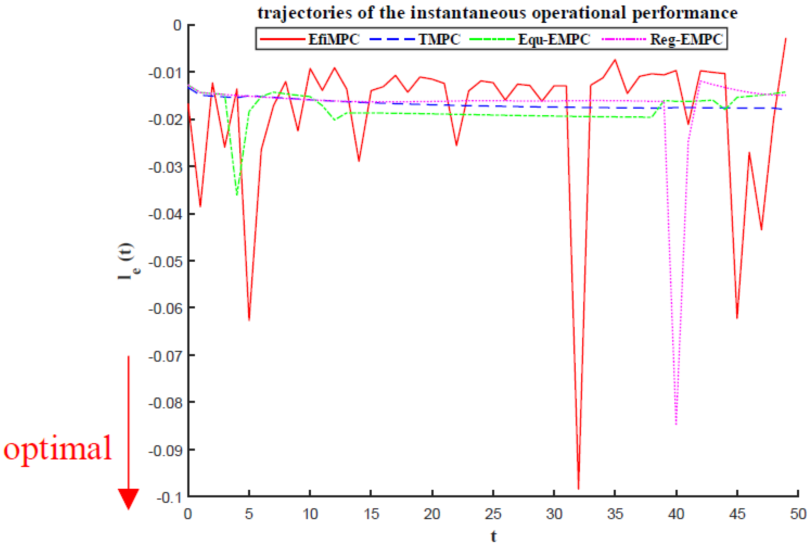
The instantaneous operation performances of the comparative control strategies are illustrated in Figure 5, and the minimum value of the instantaneous operation performance implies the optimal objective function value $l_P^{*}$. As shown in the figure, the instantaneous operation performance controlled by the TMPC strategy is almost steady. This is because the aim of the TMPC is to control the system into steady-state operation, and the operation performance is only a byproduct of this stabilization control performance; thus, a steady-state control performance will lead to a stable operation performance.

The instantaneous operational performances controlled by Equ-EMPC and Reg-EMPC are a little bit more dynamic than that controlled by TMPC, and some of the instantaneous operation performances can perform better than steady-state operation; this better dynamic operation performance mainly results from the transient operation performance optimization that exists in Equ-EMPC and Reg-EMPC.

The instantaneous operation performance controlled by EfiMPC has the best dynamic operation performance, which is better than that of Equ-EMPC and Reg-EMPC. EfiMPC also has the best instantaneous operation performance with the minimum value $l_{P,*}^{dynamic}=-0.0984<l_{P,*}^{steady}\left(x_s,u_s\right)=-0.0178$. This optimal dynamic operation performance of EfiMPC is realized by the outer level of the nested structure, where the dynamic operation of the operation performance is directly optimized at the control layer online. However, this transient superiority of EfiMPC resulting from the instantaneous operation performance alone does not mean the superiority of the optimal global performance of the whole system; thus, the closed-loop operation performances are required to further compare the global performances of the comparative control strategies.

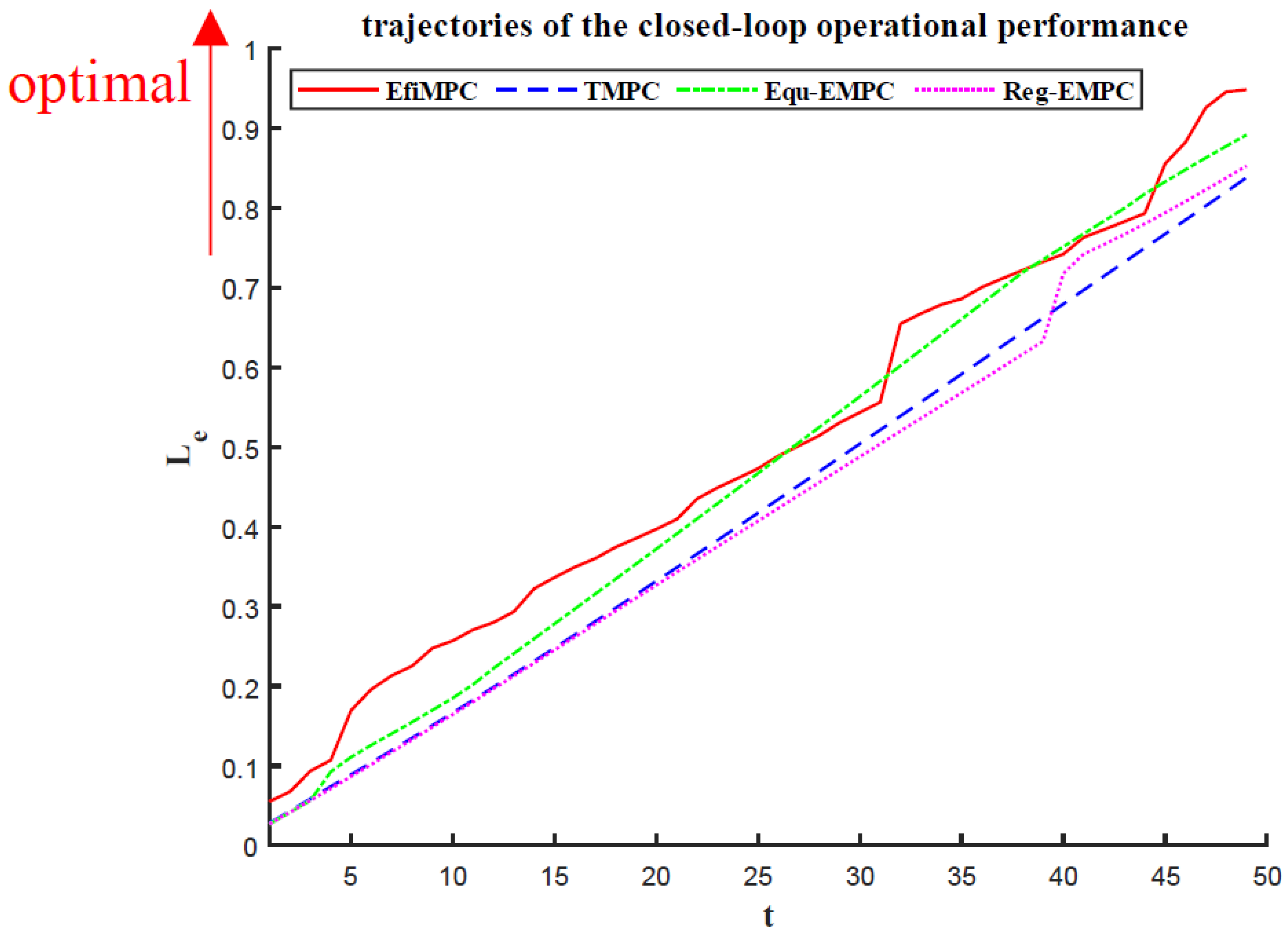
The closed-loop operation performances of the comparative control strategies are illustrated in Figure 6, and it is calculated as follows, where the maximum value of the closed-loop operation performance implies the optimum:

$$L_P={{\displaystyle \int }}_{t_0}^{t_f}-l_P\left(x\left(t\right),u\left(t\right)\right)dt$$

where $l_P\left(x\left(t\right),u\left(t\right)\right)$ represents the instantaneous operation performance, and $t_0$ and $t_f$ represent the starting instant of the CSTR process and the ending instant of the CSTR process, respectively.

As shown in Figure 6, it is clear that EfiMPC can generate the best closed-loop operation performance with the value of $L_P^{Efi}=0.9487$ (the maximum value implies the optimum), and the closed-loop operation performances controlled by TMPC, Equ-EMPC, and Reg-EMPC are $L_P^{TMPC}=0.8383$, $L_P^{Equ-EMPC}=0.8919,$ and $L_P^{Reg-EMPC}=0.8529$, respectively.

The Equ-EMPC strategy and the Reg-EMPC strategy can both outperform the TMPC strategy. This is because Equ-EMPC and Reg-EMPC both can optimize the transient operation performance, while TMPC only optimizes the control performance, and the operation performance of TMPC is heavily dependent on the steady-state operation.

The reason that EfiMPC can outperform Equ-EMPC and Reg-EMPC is that EfiMPC can not only optimize the transient operation performance in a wider search space but also guarantee that the optimized dynamic operation performance is better than the steady-state operation in the closed-loop perspective.

Thus, the effectiveness of the proposed EfiMPC has been demonstrated by the best closed-loop operation performance $L_P^{Efi}=0.9487,$ as reported in

Table 1. The closed-loop operation performance of the comparative control strategies.

	EfiMPC	TMPC	Equ-EMPC	Reg-EMPC
$L_P$	0.9487	0.8383	0.8919	0.8529

.

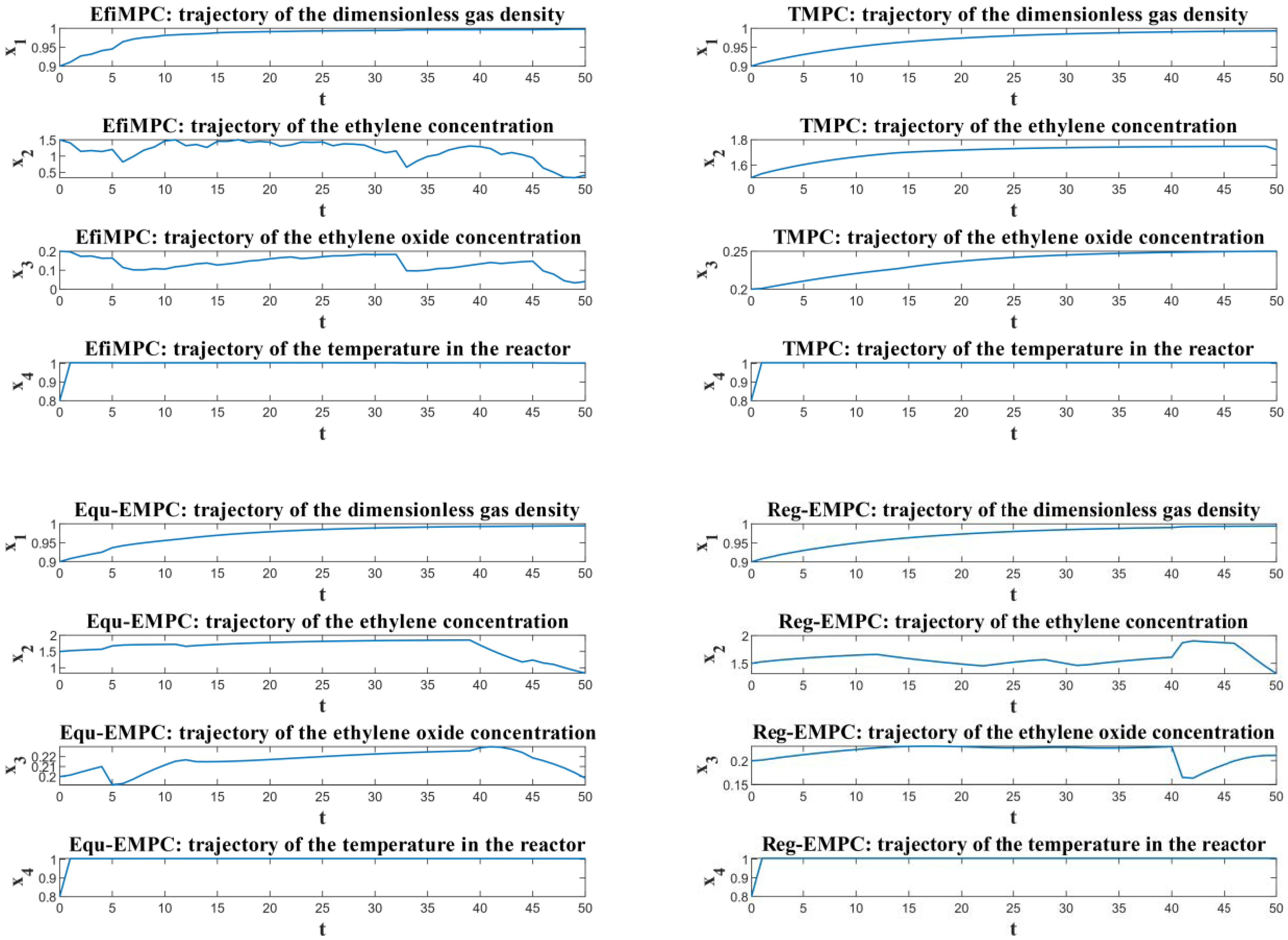
To further investigate the performances of the comparative control strategies, the state trajectories of these four comparative control strategies are illustrated in Figure 7, and the control inputs of these four comparative control strategies are illustrated in Figure 8. As shown in these two figures, after a short transient behavior period, the control actions, as well as the corresponding state trajectories controlled by TMPC, become steady, which indicates that TMPC leads to steady-state operation in this CSTR process.

Unlike TMPC, which focuses only on the control performance with respect to the optimal steady state, Equ-EMPC and Reg-EMPC both can optimize the transient operation performance before steady state, and the resulting control actions and the corresponding state trajectories thus have dynamic behaviors. However, limited by the small search space of Equ-EMPC and by the uncertain operation performance within the terminal region of Reg-EMPC, Equ-EMPC and Reg-EMPC can only optimize the dynamic operation to a small extent.

On the other hand, thanks to the nested structure of EfiMPC, it can obtain a better dynamic operation performance compared to the optimal steady-state operation online, and the control actions can perform a much more dynamic behavior with a higher frequency compared to Equ-EMPC and Reg-EMPC, as shown in Figure 8. More flexible movements of the control actions imply a higher optimization potential for closed-loop operation performance.

4.3. Discussion

Although TMPC aims only to optimize the control performance with respect to the optimal steady state $\left(x_s,u_s\right)$, it can also generate an acceptable closed-loop operation performance with $L_P^{TMPC}=0.8383$, and this operation performance is mainly guaranteed by the optimal steady state $\left(x_s,u_s\right)$ optimized by the upper RTO layer. To be specific, the upper RTO layer optimizes the global objective of the whole system $l_P$ based on a steady-state model of the controlled process. The lower advanced control layer receives this optimized set point and tries its best to stabilize the system into this steady state. Although the objective of the control layer is the control performance with respect to the given set point, the operation performance can be guaranteed in a neighborhood of the optimal steady-state operation by this control performance. Thus, although the operation performance is a byproduct of the TMPC strategy, its operation performance can be guaranteed to some extent.

Since TMPC can only guarantee the operation performance near the optimal steady-state operation, the optimization of the transient operation performance has the potential to lead to a better closed-loop operation performance, and Equ-EMPC and Reg-EMPC are introduced by researchers for this purpose. Take this CSTR process for example, $L_P^{Equ-EMPC}=0.8919$ and $L_P^{Reg-EMPC}=0.8529$ indicate that Equ-EMPC and Reg-EMPC can find a better dynamic operation than that of TMPC. However, it is necessary to mention that the improvements in Equ-EMPC and Reg-EMPC can only be achieved for the control applications where the steady-state operation is not the optimal operation and better dynamic operations exist in the controlled problem; otherwise, the superiorities of Equ-EMPC and Reg-EMPC will deteriorate.

As for the proposed EfiMPC strategy, the nested structure gives it the ability to recognize whether better dynamic operations based on the current system state exist, and it can find the optimal dynamic operation if it exists; otherwise, EfiMPC will lead to the optimal steady-state operation instead. Thus, EfiMPC can be applied to general control applications, and the operation performance can be optimized no matter if the optimal operation mode is steady-state operation or dynamic operation. In this CSTR application, EfiMPC finds the best global dynamic operation performance with $L_P^{Efi}=0.9487$.

One interesting phenomenon that appeared in the simulation is that TMPC performed a steady-state operation for most of the processing time as expected, but it led to an obvious dynamic behavior that deviated from the steady state at the end of the process operation. For example, the control action $u_2$ of TMPC had a sudden change at the end of the operation, as shown in Figure 8. This phenomenon reveals the main limitation of the TMPC strategy: since TMPC focuses only on the control performance, it ignores the transient operation behavior during the period before the steady state, and it has to compensate for this transient operation behavior at the end of the control process. On the other hand, EfiMPC takes the transient operation performance into consideration online at every sample instant; thus, EfiMPC can take advantage of these transient operation performances, leading to optimal dynamic operation.

In addition, as shown in Figure 8, the control actions of EfiMPC change frequently with large values, and the control actions of TMPC are stable most of the time. This implies that the better dynamic operation controlled by EfiMPC is realized by the dynamic control actions, which means EfiMPC sacrifices some control performance to achieve a better dynamic operation performance. If we put some constraints on the variation of the control actions, the control actions will change less frequently and to a smaller extent, but the improvements in the operation performance will suffer accordingly.

Finally,

Table 2. The online computation times of the comparative control strategies (seconds).

	EfiMPC	TMPC	Equ-EMPC	Reg-EMPC
Simulation time	0.6522	0.1688	0.4140	0.4385

illustrates the online computation times of the comparative control strategies, and their values are all smaller than the sample interval ${\mathsf{\Delta }\mathrm{t}}_{\mathrm{sam}}=1s$. As shown in Table 2, EfiMPC has the largest computation burden, and TMPC spends the least time on computation. This indicates that although the nested structure of EfiMPC can heavily improve the global operation performance, it has a larger computation burden for this improvement. In order to make EfiMPC more applicable to fast applications, future research should investigate how to reduce the computational burden of EfiMPC.

5. Conclusions

A novel control strategy that aims to improve global operation performance to realize optimal operation and control is proposed in this paper. First, the ideal EfiMPC strategy with a nested structure was proposed, where the inner layer is the offline construction of an efficiency-oriented terminal region and the outer layer is the direct optimization of the transient operation performance. This efficiency-oriented terminal region can guarantee a dynamic operation performance in the closed-loop perspective, and a better global operation performance can thus be obtained.

In order to avoid the construction of the optimal efficiency-oriented terminal region, a practical EfiMPC strategy in which the efficiency-oriented terminal region needs not to be defined explicitly is then proposed. Specifically, the inner layer in practical EfiMPC is the online optimization of the average dynamic operation performance, and it is guaranteed to perform better than the optimal steady-state operation. The inner layer in practical EfiMPC focuses mainly on the control performance to guarantee the closed-loop stability, and the outer layer focuses mainly on the free optimization of the transient operation performance; thus, practical EfiMPC integrates optimization and control into a nested structure to realize optimal control. The recursive feasibility and the closed-loop stability of practical EfiMPC were also discussed.

A CSTR process application was used to test the superiority of the proposed practical EfiMPC. Compared with the TMPC, Equ-EMPC, and Reg-EMPC strategies, practical EfiMPC generated the best global operation performance, as expected; thus, the effectiveness of the proposed EfiMPC has been demonstrated.

This paper introduces the initial idea of nested structure-based EfiMPC. For future studies, the offline construction of the optimal efficiency-oriented terminal region in ideal EfiMPC can be investigated. In addition to the average dynamic operation used in the inner layer in practical EfiMPC, other types of inner optimization problems aiming to guarantee closed-loop operation can be researched. Finally, the effectiveness of EfiMPC in applications with disturbances can be studied.